multiobjective engineering design optimization problems: a ... · universidade de são paulo 2012...

Universidade de São Paulo

2012

Multiobjective engineering design optimization

problems: a sensitivity analysis approach Pesquisa Operacional,v.32, n.3, p.575-596,2012http://www.producao.usp.br/handle/BDPI/38887

Downloaded from: Biblioteca Digital da Produção Intelectual - BDPI, Universidade de São Paulo

Biblioteca Digital da Produção Intelectual - BDPI

Departamento de Naval e Oceânica - EP/PNV Artigos e Materiais de Revistas Científicas - EP/PNV

http://www.producao.usp.br

http://www.producao.usp.br/handle/BDPI/38887

“main” — 2012/12/4 — 15:13 — page 575 — #1

Pesquisa Operacional (2012) 32(3): 575-596© 2012 Brazilian Operations Research SocietyPrinted version ISSN 0101-7438 / Online version ISSN 1678-5142www.scielo.br/pope

MULTIOBJECTIVE ENGINEERING DESIGN OPTIMIZATION PROBLEMS:A SENSITIVITY ANALYSIS APPROACH

Oscar Brito Augusto1*, Fouad Bennis2 and Stephane Caro3

Received August 5, 2011 / Accepted July 20, 2012

ABSTRACT. This paper proposes two new approaches for the sensitivity analysis of multiobjective design

optimization problems whose performance functions are highly susceptible to small variations in the design

variables and/or design environment parameters. In both methods, the less sensitive design alternatives

are preferred over others during the multiobjective optimization process. While taking the first approach,

the designer chooses the design variable and/or parameter that causes uncertainties. The designer then

associates a robustness index with each design alternative and adds each index as an objective function

in the optimization problem. For the second approach, the designer must know, a priori, the interval of

variation in the design variables or in the design environment parameters, because the designer will be

accepting the interval of variation in the objective functions. The second method does not require any law

of probability distribution of uncontrollable variations. Finally, the authors give two illustrative examples

to highlight the contributions of the paper.

Keywords: multiobjective optimization, Pareto-optimal solutions, sensitivity analysis.

1 INTRODUCTION

Many engineering design problems are multiobjective by nature, because they often involve morethan one design objective to be optimized. These design objectives impose potentially conflictingrequirements on the technical and economic performance of a given system. A designer mustformulate an optimization problem with multiple objectives if he/she wishes to study the trade-offs that exist between these conflicting objectives and to explore their design options.

Multiobjective engineering design problems often have design parameters with uncontrollablevariations due to noise or uncertainties. Such variations can affect outcomes significantly, suchas the performances of objective functions and/or the feasibility of the Pareto optimal solutions.

*Corresponding author1Escola Politecnica da Universidade de Sao Paulo – E-mails: [email protected] / [email protected] Centrale de Nantes, Institut de Recherche en Communications et Cybernetique de Nantes– E-mail: [email protected] de Recherche en Communications et Cybernetique de Nantes – E-mail: [email protected]

“main” — 2012/12/4 — 15:13 — page 576 — #2

576 MULTIOBJECTIVE ENGINEERING DESIGN OPTIMIZATION PROBLEMS

A robust optimal solution is as good as possible with regard to the objective functions, and itoffers the lowest possible sensitivity to variations in design variables and design parameters. Inpractice, all engineering designs are sensitive to uncertainties that can arise from manufactur-ing operations, variations in material properties, the operating environment and other reasons.Moreover, non-robust designs can be expensive to produce or to operate and can fail frequentlyin service.

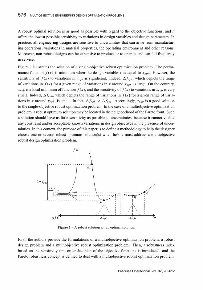
Figure 1 illustrates the solution of a single-objective robust optimization problem. The perfor-mance function f (x) is minimum when the design variable x is equal to xopt . However, thesensitivity of f (x) to variations in xopt is significant. Indeed, 1 fopt , which depicts the rangeof variations in f (x) for a given range of variations in x around xopt , is large. On the contrary,xrob is a local minimum of function f (x), and the sensitivity of f (x) to variations in xrob is verysmall. Indeed, 1 frob, which depicts the range of variations in f (x) for a given range of varia-tions in x around xrob, is small. In fact, 1 frob < 1 fopt . Accordingly, xrob is a good solutionto the single-objective robust optimization problem. In the case of a multiobjective optimizationproblem, a robust optimum solution may be located in the neighborhood of the Pareto front. Sucha solution should have as little sensitivity as possible to uncertainties, because it cannot violateany constraint and/or acceptable known variations in design objectives in the presence of uncer-tainties. In this context, the purpose of this paper is to define a methodology to help the designerchoose one or several robust optimum solution(s) when he/she must address a multiobjectiverobust design optimization problem.

Figure 1 – A robust solution vs. an optimal solution.

First, the authors provide the formulations of a multiobjective optimization problem, a robustdesign problem and a multiobjective robust optimization problem. Then, a robustness indexbased on the sensitivity first order Jacobian of the objective functions is introduced, and thePareto robustness concept is defined to deal with a multiobjective robust optimization problem.

Pesquisa Operacional, Vol. 32(3), 2012

“main” — 2012/12/4 — 15:13 — page 577 — #3

OSCAR BRITO AUGUSTO, FOUAD BENNIS and STEPHANE CARO 577

Then, two illustrative examples highlight the paper’s contributions. Finally, the conclusions arediscussed.

Nomenclature

fi (X) i th objective function

f(X) vector of objective functions

g j (X) j th inequality constraint function

K K T Karush-Khun-Tucker

Js global sensitivity Jacobian matrix

Jx sensitivity Jacobian matrix related to the design variables

Jp sensitivity Jacobian matrix related to the design parameters

k number of objective functions

m number of inequality constraint functions

n number of decision variables

q number of design parameters

pi i th design parameter

p vector of design parameters

pin f , psup lower and upper bounds of the design parameters

R(v) robustness index associated with the design variables X and the parameters p

S feasible region in the decision space

S sensitivity of the objective function

S diagonal matrix with the singular values in the singular value decomposition

U unitary matrix, expressed in the function space, in the singular value decomposition

v vector joining the design variables X and the parameters p

V unitary matrix expressed in the decision space in the singular value decomposition

xi i th decision variable

xi average of the ith decision variable included in the optimal set

X decision or design variables vector

X∗ non-dominated solution of a multiobjective optimization problem

Xin f , Xsup lower and upper bounds in the decision space

λ j weighting factor for the j th inequality constraint gradient in the K K T condition

1xio interval of a known uniformly distributed variation of the i th design variable

1pio interval of a known uniformly distributed variation of the i th design parameter

1 fio acceptable variation in the i th objective function due to 1v uncertainties

λ vector of λ js

σi standard deviation for the i th decision variable included in the optimal set

ωi weighting factor for the i th objective function gradient in the K K T condition

ω vector of ωis

∇ gradient operator


“main” — 2012/12/4 — 15:13 — page 578 — #4


2 Definitions of problems

In this section, the formulations of (i) a multiobjective optimization problem, (ii) a robust designproblem and (iii) a multiobjective robust optimization problem are given.

2.1 Multiobjective optimization problem

A general multiobjective optimization problem attempts to find the design variables X that opti-mize a vector objective function f(X) over the feasible design space S. The determination of aset of non-dominated solutions, the Pareto optimum solutions or non-inferior solutions X∗ canachieve a compromise among several objective functions. The problem formulation is defined asfollows:

minimize: f(X) (1a)

subject to: gi (X) ≤ 0, i = 1, 2, . . . m. (1b)

Xinf ≤ X ≤ Xsup (1c)

where f(X) =[

f1, f2, f3, . . . , fk]T : Rn → Rk , with fi (X) : Rn → R as a vector with the

values of objective functions to be minimized. X is the vector that contains the design variables,also called decision variables, defined in the space Rn . Xinf and Xsup are respectively the lowerand upper bounds of the design variables. gi (X) : Rn → R represents the i th inequality con-straint function. Equations (1b) and (1c) define the region of feasible solutions, S, in the decisionvariable space. The constraints gi (X) are “less than or equal” functions in view of the fact that“greater or equal” functions may be converted to the first type if they are multiplied by minus1. Similarly, the problem deals with the “minimization” of functions fi (X), given that function“maximization” can be transformed into the former by multiplying it by minus 1.

2.1.1 Pareto optimal solution

The notion of optimum in the context of solving multiobjective optimization problems is knownas “Pareto optimal”. A solution is said to be Pareto optimal if there is no alternative to improvingone objective without worsening at least one other, that is, the feasible point X∗S is Pareto optimalwhen there is no other feasible point X ∈ S so ∀i, j, fi (X) ≤ fi (X∗) with strict inequality in atleast one condition, f j (X) < f j (X∗).

Due to the conflicting nature of the objective functions, the Pareto optimal solutions are usuallyscattered in the region S, a consequence of the solutions being unable to minimize the objectivefunctions simultaneously. Solving the optimization problem achieves a set of Pareto optimalsolutions defined in the decision space, after which an image of the objective functions, alongwith the Pareto front, is calculated over the set of optimal solutions.

In general, solving a multiobjective optimization problem is not as simple as solving any scalarproblem. According to Schaffer (1985), Goldberg (1989) and Deb (2001), evolutionary algo-rithms are usually best suited to determining the Pareto front.


“main” — 2012/12/4 — 15:13 — page 579 — #5


2.1.2 Necessary conditions for Pareto optimality

Optimizing the multiobjective problems that are expressed by Eqs. (1a-1c) are of general char-acter, because the equations represent the problem of single-objective optimization when k = 1.According to Miettinen (1998), as in single-objective optimization problems, the solution X∗ ∈ Sfor the Pareto optimality must satisfy the Karush-Kuhn-Tucker condition, expressed as:

k∑

i=1

ωi∇ fi (X∗) +

m∑

j=1

λ j∇g j (X∗) = 0 (2a)

λ j g j (X∗) = 0 (2b)

λ j ≥ 0 (2c)

ωi ≥ 0;k∑

i=1

ωi = 1 (2d)

where ωi is the weighting factor, positive, for the gradient of the i th objective function, calculatedat point X∗, ∇ fi (X∗). λ j represents the weighting factor for the gradient of the j th inequalityconstraint function ∇g j (X∗). It is zero when the associated constraint function is not active, i.e.,g j (X∗) < 0.

It should be emphasized that the set of Eqs. (2a) to (2d) form the necessary conditions for X∗ tobe Pareto optimal.

2.2 Robust design problem

The concept of robust design was first used by Taguchi (1993). He introduced the concept ofparameter design to improve the quality of a product whose manufacturing process involvessignificant variability or noise. Robust design aims at minimizing the sensitivity of performanceto variations without controlling the causes of these variations. In the last decades, several authorscontributed to the formulation and the improvement of robust design problems.

To deal with robustness, a set of design parameters p =[

p1, p2, p3, . . . pq]T should be consid-

ered. Those parameters cannot be adjusted by the designer and are thus uncontrollable, such asthe cost of the steel used in ship construction. The design variables

X =[x1, x2, x3, . . . xn

]T

can also be subjected to uncontrollable variations for the reasons of manufacturing errors, wear-ing or other uncertainties, although their nominal value is fixed.

A general multiobjective robust design optimization problem aims to find the design variablesthat optimize a vector objective function, f(X, p), and to minimize its range of variations1f(X, p) =

[1 f1,1 f2,1 f3, . . . 1 fk

]T over the feasible design space S. The determination ofa set of non-dominated solutions achieves a compromise among several objective functions that


“main” — 2012/12/4 — 15:13 — page 580 — #6


consider variations in the design variables and parameters. Calling vT =[XT pT

], the problem

formulation can be defined as follows:

minimize: f(X, p), (3a)

1f(X, p)

over X =[x1, x2, x3, . . . xn

]T (3b)

subject to: gi (X, p) + 1gi (X, p) ≤ 0, i = 1, 2, . . . m. (3c)

Xinf ≤ X ≤ Xsup (3d)

v − 1vinf ≤ v ≤ v + 1vsup (3e)

All sets of equation (3) are general for search robust solutions of multiobjective optimizationproblems.

Sundaresan et al. (1993) developed a procedure that incorporates uncertainties in design vari-ables and variations in constraints due to these uncertainties. Chase et al. (1996) presented thedirect linearization method for tolerance analyses of 2D and 3D mechanical assemblies. Chenet al. (1996) studied two broad categories of problems, namely, (i) Type 1 problems, whichminimize variations in performance caused by variations in noise factors (uncontrollable param-eters), and (ii) Type 2, which minimize variations in performance caused by variations in controlfactors (design variables). Ben-Tal and Nemirovski (1998, 2002) proposed a study of convexoptimization problems for which the data, in the present notation p, is not specified exactly.Instead, the data are known only to belong to a given uncertainty set. They developed models foruncertain Linear, Conic Quadratic and Semidefinite programming problems. Kalsi et al. (2001)introduced a technique to reduce the effects of uncertainty and incorporated flexibility in thedesign of complex engineering systems involving multiple decision makers. Parkinson (2000)used a deterministic method of robust design to determine the optimum nominal dimensions ofan assembly in order to improve the assembly quality. Bertsimas et al. (2004) have proposeda robust constrained optimization method for linear programming problems where the matrix ofcoefficients belongs to a known uncertainty set that is bounded. They have shown that this kindof problem is still linear programming. Bertsimas and Sim (2004) also focused on linear pro-gramming problems, seeking to reduce the level of conservatism of the robust solutions in termsof probabilistic bounds of constraint violations. They have shown that their method retains theadvantages of the linear framework and offers full control over the degree of conservatism forevery constraint. Thus, their method provides a probabilistic guarantee that the robust solutionwill be feasible with high probability.

The solutions of the presently proposed methods will always be feasible, and all nominal valuesof problem parameters, p, are known. For the first method, described in section 3.1, no additionalinformation is needed to search the less sensitive solutions under variations of p and eventuallyvariations in the decision variables X. For the second method, described in the section 3.2, thesevariations must be bounded. Both of these methodologies can be incorporated in any nonlinearmultiobjective optimization algorithm.


“main” — 2012/12/4 — 15:13 — page 581 — #7


In the next section, the authors propose a simplified approach to searching for less sensitivealternatives when solving multiobjective optimization problems.

3 A SIMPLIFIED MULTIOBJECTIVE ROBUST OPTIMIZATION PROBLEM

Given that a robust optimal solution is as good as possible with regard to the objective functionsand that it is as least sensitive as possible to variations in design variables and design parameters,this section presents two methods where robust design alternatives are preferred over othersduring the multiobjective optimization process.

First, the designer chooses only the design variables and/or design parameters that are subject tovariations. With this information, a Robustness Index is associated with each design alternative.This index is added as one more function to be optimized. In the second approach, the designeraccepts variations in the performance functions, limited in fixed intervals, knowing a priori therange of variations in the design variables and in the design parameters.

Assuming that f is of class C2 in v, one can expand Eq. (3a) in the neighborhood of the point v0

and keep only the linear terms. Then, the following equation can be obtained:

δf = Jsδv + e(‖δv‖2) (4a)

δvT =[δXT δpT ]

(4b)

Jx = ∂f/∂X (4c)

Jp = ∂f/∂p (4d)

Js =[Jx Jp

](4e)

where ‖ ∙‖2 denotes the Euclidian norm operator and e(v) an error function. Js is the globalsensitivity Jacobian matrix, and it describes the effect of the variations in design variables anddesign parameters to the performance functions. δX and δp are the variations in the designvariables and in the design parameters, respectively. Jx is the (k × n) sensitivity Jacobian matrixof f(v) with respect to X, and Jp is the (k × q) sensitivity Jacobian matrix of f(v) with respectto p, respectively. If variations in the design variables are not considered, then Js = Jp. Ifvariations in design parameters are not considered, then Js = Jx .

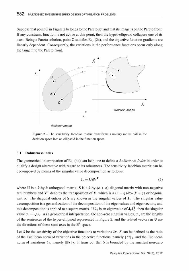
Ignoring the error in Eq. (4a), an approach to a robust solution is defined as one that is as leastsensitive as possible to any variations in the decision variables and design parameters in its neigh-borhood. Considering 1v as a closed normalized unit hyper-sphere centered at point v in theEuclidean space Rn+q , i.e., ‖1v‖2 = 1, then Js is a linear application that maps the hyper-sphere in a hyper-ellipsoid in the normalized function space, centered in f(v) and described bythe variations 1f(v) ∈ Rk . In Figure 2, three design alternatives are checked for their sensitivityin the decision variable space. Since the local perturbation in the neighborhood of point A causesa large modification in the objective values, this alternative may not be as robust as the alternativeB, because the latter does not bring on a large change in objective values, even in the presence ofa local perturbation in its vicinity.


“main” — 2012/12/4 — 15:13 — page 582 — #8


Suppose that point C in Figure 2 belongs to the Pareto set and that its image is on the Pareto front.If any constraint function is not active at this point, then the hyper-ellipsoid collapses one of itsaxes. Being a Pareto solution, point C satisfies Eq. (2a), and the objective function gradients arelinearly dependent. Consequently, the variations in the performance functions occur only alongthe tangent to the Pareto front.

Figure 2 – The sensitivity Jacobian matrix transforms a unitary radius ball in the

decision space into an ellipsoid in the function space.

3.1 Robustness index

The geometrical interpretation of Eq. (4a) can help one to define a Robustness Index in order toqualify a design alternative with regard to its robustness. The sensitivity Jacobian matrix can bedecomposed by means of the singular value decomposition as follows:

Js = USVT (5)

where U is a k-by-k orthogonal matrix, S is a k-by-(k + q) diagonal matrix with non-negativereal numbers and VT denotes the transposition of V, which is a (n + q)-by-(k + q) orthogonalmatrix. The diagonal entries of S are known as the singular values of Js. The singular valuedecomposition is a generalization of the decomposition of the eigenvalues and eigenvectors, andthis decomposition is applied to a square matrix. If λi is an eigenvalue of JsJT

s , then the singularvalue σi =

√λi . As a geometrical interpretation, the non-zero singular values, σi , are the lengths

of the semi-axes of the hyper-ellipsoid represented in Figure 2, and the related vectors in U arethe directions of these semi axes in the Rk space.

Let S be the sensitivity of the objective functions to variations δv. S can be defined as the ratioof the Euclidean norm of variations in the objective functions, namely ‖δf‖2, and the Euclideannorm of variations δv, namely ‖δv‖2. It turns out that S is bounded by the smallest non-zero


“main” — 2012/12/4 — 15:13 — page 583 — #9


singular value σmin and the largest singular value σmax of its global sensitivity Jacobian matrix,Js, namely,

σmin ≤ S =‖δf‖2

‖δv‖2≤ σmax (6)

Equation (6) shows that the lower σmax is, the lower the upper bound of S will be. Accord-ingly, the Euclidean norm of Js, that is, its maximum singular value, can be used as a relevantRobustness Index:

R(v) = σmax (7)

R(v) makes sense if and only if the terms of Js are normalized, that is, if they have the same unit.Indeed, the singular values of Js cannot be compared if their units are different.

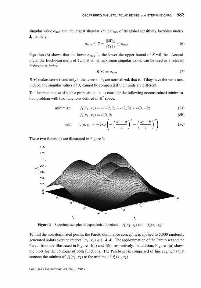
To illustrate the use of such a proposition, let us consider the following unconstrained minimiza-tion problem with two functions defined in R2 space:

minimize: f1(x1, x2) = c(−2, 2) + c(2, 2) + c(0, −2), (8a)

f2(x1, x2) = c(0, 0) (8b)

with c(a, b) = − exp

(

−(

x1 − a

2

)2

−(

x2 − b

2

)2)

(8c)

These two functions are illustrated in Figure 3.

Figure 3 – Superimposed plot of exponential functions − f1(x1, x2) and − f2(x1, x2).

To find the non-dominated points, the Pareto dominance concept was applied to 5,000 randomlygenerated points over the interval (x1, x2) ∈ [−4, 4]. The approximation of the Pareto set and thePareto front are illustrated in Figures 4(a) and 4(b), respectively. In addition, Figure 4(a) showsthe plots for the contours of both functions. The Pareto set is comprised of line segments thatconnect the minima of f1(x1, x2) to the minima of f2(x1, x2).


“main” — 2012/12/4 — 15:13 — page 584 — #10


Figure 4 – Nominal approximations of the Pareto set and Pareto front for minimization of the exponential

functions f1(x1, x2) and f2(x1, x2).

To search robust solutions, the authors applied the robust multi-objective optimization procedureby adding the robustness index, as defined by Eq. (7), as a third objective function. The robustproblem can be written as

minimize: f1(x1, x2) = c(−2, 2) + c(2, 2) + c(0, −2) and (9a)

f2(x1, x2) = c(0, 0); and (9b)

f3(x1, x2) = R(x1, x2) = σmax (9c)


(

−(

x1 − a

2

)2

−(

x2 − b

2

)2)

(9d)

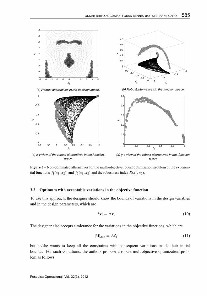
The non-dominated points are shown in Figure 5. Clouds of points lie both near the nominalPareto set and far away from it. In the specific problem, both functions are nearly flat in thoseregions. Accordingly, the robustness indexes for these points are very low, placing them as non-dominated although their function values are non-optimal compared to those near the nominalPareto set.

Given the flat regions in Figure 3, one can conclude that the robustness index, when includedin the multi-objective optimization problem as an additional objective function to be minimized,permits the location of the less sensitive non-dominated alternatives. Moreover, it naturally dis-perses the nominal Pareto front of the original problem, causing the decision-making process tobecome even more difficult.

To overcome this difficulty, the authors suggest in the next section a complementary approach todealing with robustness in multi-objective optimization problems.


“main” — 2012/12/4 — 15:13 — page 585 — #11


Figure 5 – Non-dominated alternatives for the multi-objective robust optimization problem of the exponen-

tial functions f1(x1, x2), and f2(x1, x2) and the robustness index R(x1, x2).

3.2 Optimum with acceptable variations in the objective function

To use this approach, the designer should know the bounds of variations in the design variablesand in the design parameters, which are

|δv| = 1v0 (10)

The designer also accepts a tolerance for the variations in the objective functions, which are

|δf|acc = 1f0 (11)

but he/she wants to keep all the constraints with consequent variations inside their initialbounds. For such conditions, the authors propose a robust multiobjective optimization prob-lem as follows:


“main” — 2012/12/4 — 15:13 — page 586 — #12


minimize: f(v) (12a)

over X

subject to: gi (v) + 1gi (v) ≤ 0, i = 1, 2, . . . m. (12b)

|δf(v)| − 1f0 ≤ 0 (12c)

Xinf ≤ X ≤ Xsup (12d)

with |δv| = 1v0 (12e)

By using this approach, one can state the optimization problem with two exponential objectivefunctions as:

minimize: f1(x1, x2) = c(−2, 2) + c(2, 2) + c(0, −2) and (13a)

f2(x1, x2) = c(0, 0) (13b)

subject to: |δ(x1, x2)| − 1 f10 ≤ 0 (13c)

|δ f2(x1, x2)| − 1 f20 ≤ 0 (13d)

1(x1, x2)0 = 0.1 (13e)


(

−(

x1 − a

2

)2

−(

x2 − b

2

)2)

(13f)

where the acceptable function variations are set to 1 percent without loss of generality, and theyinclude variations in the design variables that are equal to 10 percent of their nominal value.Figure 6 shows the Pareto optimal solutions plotted in the design space and the Pareto frontapproximation obtained by using the random walk over the design space.

Considering the acceptable values used, the robust Pareto front is less performing than the nom-inal one.

In the classical sensitivity analysis, the problems may have data (p, in the present notation) thatare not specified exactly and are only known to belong to a given uncertainty set.

With the proposed methods, one can approach the engineering design optimization problemwhile considering the effects of uncertainty. The idea behind these methods is to consider thatsome data relating to engineering problems have variations around their nominal values. More-over, the problems’ data cannot be implemented exactly even if the data are certain and an optimalsolution X∗ can be computed exactly.

4 APPLICATIONS

This section presents two engineering examples to demonstrate the proposed multiobjective ro-bust optimization. The first problem deals with the design of a vibrating platform. This prob-lem includes six design variables with one being combinatorial; it also has five constraintsand two uncontrollable parameters. This example should highlight the influence of the discretevariable in the robust search. The second problem deals with the conceptual design of a ship.


“main” — 2012/12/4 — 15:13 — page 587 — #13


Figure 6 – Non-dominated points for the robust multi-objective optimization problem of the exponential

objective functions f1(x1, x2), and f2(x1, x2) with 1(x1, x2)0 = 0.1 and 1 f10 = 1 f20 = 0.01.

It contains six design variables, 21 constraints and three uncontrollable parameters, and it repre-sents a more realistic problem that naval architects are likely to face.

To solve both problems, one will need a method to find the Pareto front for multiobjective op-timization problems. The most widespread method in the literature is the genetic algorithm.Originally proposed by Holland (1975) for applications engaged with control theories, it wasaccepted quickly into numerous areas of engineering and science. Coello (2010) maintains anupdated list of publications involving the genetic algorithm.

Many versions of genetic algorithms have served as meta-algorithms in the literature. The onethat appears in this work was adapted from Deb et al. (2000), which is the Non-dominated Sort-ing Genetic Algorithm, version II (NSGA II). This version is easy to use and depends on only twoparameters: the number of chromosomes in the population and the number of generations thatthis population will evolve. With each evolution, the non-dominated solutions in the populationconverge toward the Pareto optimal solutions.

4.1 Problem 1: design of a vibrating platform

To illustrate the proposed robust approach, the authors present the engineering problem adaptedfrom Gunawan and Azarm (2005).

This problem aims to optimize the design of a platform modeled as a pinned-pinned sandwichbeam with a vibrating motor on top, as shown in Figure 7. The platform has three layers (aninner layer, two middle layers sandwiching the inner layer and two outer layers sandwiching theinner and middle layers) of material. The layers must be comprised of three different materialsthat are named A, B and C , and the choice of materials for the layers must be mutually exclu-sive so that two layers do not use the same material. However, the thickness of some layerscan be null.


“main” — 2012/12/4 — 15:13 — page 588 — #14


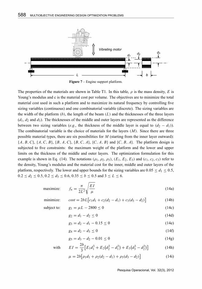
Figure 7 – Engine support platform.

The properties of the materials are shown in Table T1. In this table, ρ is the mass density, E isYoung’s modulus and c is the material cost per volume. The objectives are to minimize the totalmaterial cost used in such a platform and to maximize its natural frequency by controlling fivesizing variables (continuous) and one combinatorial variable (discrete). The sizing variables arethe width of the platform (b), the length of the beam (L) and the thicknesses of the three layers(d1, d2 and d3). The thicknesses of the middle and outer layers are represented as the differencebetween two sizing variables (e.g., the thickness of the middle layer is equal to (d2 − d1)).The combinatorial variable is the choice of materials for the layers (M). Since there are threepossible material types, there are six possibilities for M (starting from the inner layer outward):{A, B, C}, {A, C, B}, {B, A, C}, {B, C, A}, {C, A, B} and {C, B, A}. The platform design issubjected to five constraints: the maximum weight of the platform and the lower and upperlimits on the thickness of the middle and outer layers. The optimization formulation for thisexample is shown in Eq. (14). The notations (ρ1, ρ2, ρ3), (E1, E2, E3) and (c1, c2, c3) refer tothe density, Young’s modulus and the material cost for the inner, middle and outer layers of theplatform, respectively. The lower and upper bounds for the sizing variables are 0.05 ≤ d1 ≤ 0.5,0.2 ≤ d2 ≤ 0.5, 0.2 ≤ d3 ≤ 0.6, 0.35 ≤ b ≤ 0.5 and 3 ≤ L ≤ 6.

maximize: fn =π

2L2

√E I

μ(14a)

minimize: cost = 2bL[c1d1 + c2(d2 − d1) + c3(d3 − d2)

](14b)

subject to: g1 = μL − 2800 ≤ 0 (14c)

g2 = d1 − d2 ≤ 0 (14d)

g3 = d2 − d1 − 0.15 ≤ 0 (14e)

g4 = d2 − d3 ≤ 0 (14f)

g5 = d3 − d2 − 0.01 ≤ 0 (14g)

with E I =2b

3

[E1d3

1 + E2(d3

2 − d31

)+ E3

(d3

3 − d32

)](14h)

μ = 2b[ρ1d1 + ρ2(d2 − d1) + ρ3(d3 − d2)

](14i)


“main” — 2012/12/4 — 15:13 — page 589 — #15


Table T1 – Properties of the beam materials.

Material A Material B Material C

ρ(kg/m3)

100.0 2770 7780

E(G Pa) 1.6 70 200

c(m3)

500.0 1500 800

It is assumed that there are uncontrollable variations in the density of material A (ρA) and cost ofmaterial B (cB), and the optimum solutions must be as minimally sensitive as possible to thesevariations. Moreover, the designer wants to obtain the robust Pareto solutions to this problem forthe nominal parameter values ρA = 100 kg/m3 and cB = 1500 $/m3.

The variations in the parameters affect the two objective functions and the platform weight, andthis effect is incorporated in the constraint function g1. To take into account the feasibility of therobust search process, the following constraint functions were added.

g6 = |1cost| − 1cost0 ≤ 0 (15a)

g7 = |1 f n| − 1 f n0 ≤ 0 (15b)

g8 = g1 + |1g1| ≤ 0 (15c)

where, for the sensitivity requirements, the acceptable relative variations in objective functions1 f n0

fnand 1cost0

cost were arbitrarily set in the values shown in Figure 8 with maximum variation

for the parameters of material A defined by 1ρAρA

= 1cAcA

= 0.05. The variation related to theconstraints expressed in Eqs. (15a-15c) were calculated for the extreme points of the intervalcomposed by the parameter with its variation.

In Figures (8a-8b), the nominal Pareto set of the problem (without the uncontrollable variations)and the Pareto set obtained using the robust approach are displayed. When the robustness index isconsidered as the third objective function, the non-dominated points (square points) are dispersedover the function space, barely touching the nominal Pareto front. Therefore, the nominal Paretofront is not robust.

As expected, if the nominal solution is not robust, then different Pareto fronts will be obtained,because the acceptable variations in objective functions are modified. Table T2 shows the statis-tics for the results with different levels of these acceptable variations. This table displays somenotable facts. First, in each Pareto set, all alternatives resulted with the same material sequenceorder. Second, the material order in the nominal Pareto set is from the cheapest to the mostexpensive material as well as from the inner, thicker layer to the external, thinner layer, respec-tively, which was also expected. Third, the platform cost variation due to maximum variations inmaterial A is more relevant than the frequency variation, so one can say that the nominal Paretofront is robust from the point of view of natural frequency. Fourth, the nominal Pareto set hasthe platform cost variation at an average value of 4.51 percent with a standard deviation of 0.21percent, which means that this set will be changed and the nominal Pareto front will be movedto a less performing region if the acceptable level of cost variations is set to the lower values,


“main” — 2012/12/4 — 15:13 — page 590 — #16


as shown in Figures (8c-8d). Finally, as long as the order of the material in the platform layers’cross section is acting as a design variable, the robust Pareto fronts will exhibit the behaviorshown in Figure 8c. The fronts with a relatively small variation in restrictive acceptable cost willfall in a better region than the fronts with more flexible bounds.

Figure 8 – Nominal and robust Pareto fronts of the platform design problem.

Table T2 – Statistics for design cases varying 1 fio/ fi and material code as free design variable.

dv → b(m) L(m) d1(m) d2(m) d3(m) Material 1 fn/ fn(%) 1cost/cost(%)

1 fio ↓ b σb L σL d1 σd1 d2 σd2 d3 σd3code∗

1 fn σ1 f n 1cost σ1cost

nominal 0.35 2% 3.00 0% 0.33 29% 0.35 30% 0.35 31% 2 0.55 0.48 4.51 0.21

1% 0.35 0% 3.00 0% 0.17 44% 0.28 17% 0.28 17% 4 0.00 0.00 0.00 0.00

2% 0.35 0% 3.00 0% 0.23 56% 0.30 23% 0.31 23% 3 0.05 0.06 0.80 0.82

3% 0.35 0% 3.00 0% 0.18 59% 0.26 17% 0.27 17% 3 0.08 0.08 1.09 0.99

4% 0.35 0% 3.00 0% 0.25 17% 0.28 16% 0.28 17% 2 0.20 0.02 3.99 0.01

∗code: 1 = {A, B, C}, 2 = {A, C, B}, 3 = {B, A, C}, 4 = {B, C, A}, 5 = {C, A, B} and 6 = {C, B, A}.


“main” — 2012/12/4 — 15:13 — page 591 — #17


Furthermore, the proposed sensitivity approach is useful for characterizing robust Pareto fronts.With this approach, one can easily achieve the robust Pareto front. This approach does not requirestochastic treatment for obtaining the variations, and it does not need a probability distributionfor the variations in the design variables and design parameters.

4.2 Problem 2: preliminary design of a bulk carrier

The second application of the developed methodology is the preliminary design of a bulk carrier.The design of a vessel is not a trivial task. For decades, this problem has been handled in twoways. Some designers have adjusted a known design so that it meets new requirements, andothers have relied on simplified mathematical models controlled by an optimization algorithm,which allow them to obtain the optimal solution based on previously established technical oreconomic criteria.

This work considers the second alternative with the aid of the mathematical model for designingbulk carriers, which was developed by Pratyush and Yang (1998) and presented in detail in Au-gusto et al. (2012) study. The model comprises a set of functions that define the vessel attributes.These functions constrain the design variables of the objective functions to be optimized as wellas the space of these design variables. These functions characterize the technical and economicperformance of the ship and allow designers to evaluate each design alternative. The economicperformance of the ship refers to its annual unitary transportation cost and its annual transportedcargo, and the technical performance of the ship refers to the functions of the vessel’s design vari-ables, including length, beam, depth, draft, block coefficient and speed, which are respectively(L , B, D, T , Cb and VK ). Pratyush and Yang chose to minimize the annual transportation cost,maximize the amount of annual cargo and minimize the vessel’s weight. The present work chosethe optimization of the first two with no loss of generality. These two functions are conflicting,as shown in Figures 9 and 10.

The authors applied the proposed multiobjective robust optimization to the ship’s design in orderto consider the isolated variation in each design variable and in each design parameter for the twoapproaches. First, the Robustness Index was added as a third objective function to the original bi-objective optimization problem. Then, the variations relative to the nominal value of the designvariable and to the design parameter were arbitrarily preset at 1xio = 1 percent and 5 percent,respectively, and the consequent variations of the objective functions were limited to 1 fio andarbitrarily set at values ranging from 1 percent to 4 percent relative to their resultant or nominalvalues, depending on the case.

Figure 9 displays the results for the robust optimization related to the uncontrollable variationsin each design variable. Each figure displays the nominal (non-robust) Pareto front, the robustPareto front considering the Robustness Index as the third objective function to be minimized andthe Pareto front considering different levels of acceptable variations in the objective functions asan effect of a design variable’s uncontrollable variation around its nominal value.


“main” — 2012/12/4 — 15:13 — page 592 — #18


Figure 9 – Nominal and robust Pareto fronts for the minimization of transportation cost (CT ) and maxi-

mization of annual transported cargo (AC ), allowing isolated variations in the design variables of (L , B, D,

T , Cb and VK ).


“main” — 2012/12/4 — 15:13 — page 593 — #19


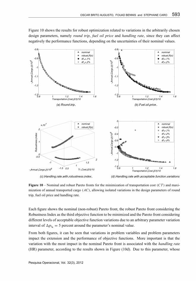
Figure 10 shows the results for robust optimization related to variations in the arbitrarily chosendesign parameters, namely round trip, fuel oil price and handling rate, since they can affectnegatively the performance functions, depending on the uncertainties of their nominal values.

Figure 10 – Nominal and robust Pareto fronts for the minimization of transportation cost (CT ) and maxi-

mization of annual transported cargo (AC), allowing isolated variations in the design parameters of round

trip, fuel oil price and handling rate.

Each figure shows the nominal (non-robust) Pareto front, the robust Pareto front considering theRobustness Index as the third objective function to be minimized and the Pareto front consideringdifferent levels of acceptable objective function variations due to an arbitrary parameter variationinterval of 1pio = 5 percent around the parameter’s nominal value.

From both figures, it can be seen that variations in problem variables and problem parametersimpact the extension and the performance of objective functions. More important is that thevariation with the most impact in the nominal Pareto front is associated with the handling rate(HR) parameter, according to the results shown in Figure (10d). Due to this parameter, whose


“main” — 2012/12/4 — 15:13 — page 594 — #20


nominal value is set to 8,000 t/day, the nominal Pareto front is very sensitive. For acceptablelevels of variations in objective functions over the interval 1 fio ∈ [1%, 3%], the respective Paretofronts practically collapse to a single solution in each respective front. This single solution willbe partially robust if the acceptable levels of variations are higher, namely 1 fio = 4 percent,when compared to those observed in the results obtained with uncontrollable variations in thedesign variables and other design parameters.

Therefore, this parameter plays an important role in the design process, because its impact on theobjective functions can degrade drastically the performance of the designed ship.

5 CONCLUSIONS

Most engineering design problems are multiobjective and contain antagonistic objective func-tions. To solve such problems, many researchers developed methods that helped them to searchfor a general solution. They have frequently elected to use evolutionary methods to locate a set ofsolutions of multiobjective optimization problems. These algorithms provide a discrete pictureof the Pareto front in the function space.

This paper introduced a new concept of a sensitivity index to perform multiobjective robustdesign optimizations, mainly when performance functions are highly sensitive to the variationsin the design variables and in the design parameters.

To introduce the concept, the authors presented formulations of a multiobjective optimizationproblem, a robust design problem and a multiobjective robust optimization problem. A robust-ness index was introduced in order to classify the nominal Pareto front as either non-sensitiverobust or not. This robustness index is based on the singular values of the sensitivity Jacobianmatrix involving the objective functions, and it is considered an additional function to be mini-mized in the optimization problem. If the nominal Pareto front is not robust, then the new front,in view of the robustness index, will be scattered in the function space.

In addition, this paper proposed a supplementary method for searching for the robust Paretofront in instances where the design variables and design parameters have known uncontrollablevariations bounded in single intervals and the designer will accept a range of these variations inthe objective functions. During this search for optimal solutions, the designer constrains varia-tions in objective functions to the acceptable intervals. The feasibility of the nominal problem ismaintained once the effects of the variations in the constraint functions are considered.

Finally, two examples illustrated the contributions of the paper. First, the proposed method wasapplied to the design of an engine support platform, a problem with two objective functions,six design variables, five constraints and uncontrollable variations in the design parameters ofmaterial cost and material density. Then, a preliminary ship design, a problem with six designvariables, two objective functions and twenty-one constraints, was conducted in a robust condi-tion considering uncontrollable variations in the design variables and in the design parameters.The authors concluded that the nominal optimal set is not robust, because one of the ship’s de-sign parameters (the port handling rate) had a significant impact on the performance of the good


“main” — 2012/12/4 — 15:13 — page 595 — #21


under design. Given the results of both illustrations, the proposed methodology appears to be asimple and useful tool for conducting robust engineering designs.

REFERENCES

[1] AUGUSTO O, BENNIS F & CARO S. 2012. A new method for decision making in multi-objective

optimization problems. Pesquisa Operacional, in press.

[2] BEN-TAL A & NEMIROVSKI A. 1998. Robust convex optimization. Mathematics of Operations

Research, 23(4): 769–805.

[3] BEN-TAL A & NEMIROVSKI A. 2002. Robust optimization – Methodology and applications.

Mathematical Programming, 92(3): 453–480.

[4] BERTSIMAS D, PACHAMANOVA D & SIM M. 2004. Robust linear optimization under general norms.

Operations Research Letters, 32: 510–516.

[5] BERTSIMAS D & SIM M. 2004. The price of robustness. Operations Research, 52(1): 35–53.

[6] CARO S, BINAUD N & WENGER P. 2008. Sensitivity analysis of planar parallel manipulators.

Proceedings of ASME Design Engineering Technical Conferences, August 3-6, New York,

NY, U.S.

[7] CHASE K, GAO J, MAGLEBY SP & SORENSEN CD. 1996. Including geometric feature variations

in tolerance analysis of mechanical assemblies. IIE Transactions, 28: 795–807.

[8] CHEN W, ALLEN JK, TSUI K-L & MISTREE F. 1996. A procedure for robust design: minimizing

variations caused by noise factors and control factors. ASME Journal of Mechanical Design, 118:

478–485.

[9] COELLO CAC. 2010. List of references on evolutionary multiobjective optimization.

http://www.lania.mx/∼ccoello/EMOO/EMOObib.html. Last accessed April 24, 2010.

[10] DEB K, AGRAWAL S, PRATAB A & MEYARIVAN T. 2000. A fast elitist non-dominated sorting

genetic algorithm for multiobjective optimization. Technical Report 200001 NSGA-II, KanGAL.

[11] DEB K. 2001. Multiobjective Objective Optimization using Evolutionary Algorithms. San Francisco:

Wiley & Sons, Ltd.

[12] GIASSI A, BENNIS F & MAISONNEUVE JJ. 2004. Multidisciplinary design optimization and

robust design approaches applied to concurrent design. International Journal of Structural and

Multidisciplinary Optimization, ISSMO, 28: 356–371.

[13] GOLDBERG D. 1989. Genetic Algorithms in Search and Machine Learning. Reading: Addison

Wesley.

[14] GUNAWAN S & AZARM S. 2005. Multiobjective robust optimization using a sensitivity region

concept. Structural Multidisciplinary Optimization, 29: 50–60.

[15] HOLLAND J. 1975. Adaptation in Natural and Artificial Systems. Ann Arbor: University of Michigan

Press.

[16] KALSI M, HACKER K & LEWIS K. 2001. A comprehensive robust design approach for decision

trade-offs in complex systems design. ASME Journal of Mechanical Design, 121: 1–10.

[17] MIETTINEN KM. 1998. Nonlinear Multiobjective Optimization. New York: Springer.


“main” — 2012/12/4 — 15:13 — page 596 — #22


[18] PARKINSON DB. 2000. The application of a robust design method to tolerancing. ASME Journal of

Mechanical Design, 22: 149–154.

[19] PRATYUSH S & YANG JB. 1998. Multiple Criteria Decision Support in Engineering Design. New

York: Springer.

[20] SCHAFFER JD. 1985. Multiple objective optimization with vector evaluated genetic algorithms. In:

Proceedings of the First International Conference on Genetic Algorithms and their Applications

[edited by J.J. Grefenstette], Psychology Press, 93–100.

[21] SUNDARESAN S, ISHII K & HOUSER DR. 1993. A robust optimization procedure with variations

on design variables and constraints. Advances in Design Automation, 1: 379–386.

[22] TAGUCHI G. 1993. On Robust Technology Development: Bringing Quality Engineering Upstream.

New York: ASME Press.


multiobjective engineering design optimization problems: a ... · universidade de são paulo 2012...

Documents