multinomial logistic regression - nutritionista · 5 logit models for multinomial logit let...

Multinomial Logistic Regression

stat 557Heike Hofmann

Outline

• Ordinal Co-variates

• Baseline Categorical Model

• Proportional Odds Logistic Regression

Example: Alcohol during pregnancy

• Observational Study: at 3 months of pregnancy, expectant mothers asked for average daily alcohol consume.infant checked for malformation at birth

Problem with deviance: if X continuous, deviance has no longer χ2 distribution. The approximation as-sumptions are violated two-fold: even if we regard X to be categorical (with lots of categories) these means,that we end up with a contingency table that has lots of small cells - which means, that the χ2 approxima-tion does not hold. Secondly, if we increase the sample size, most likely the number of different values of Xincreases, too, which makes the corresponding contingency table change size (so we cannot even talk aboutan asymptotic distribution for the smaller contingency table, as it doesn’t exist anymore once the samplesize is larger).

Model Checking by Grouping To get around the problems with the distribution assumption of G2, wecan group the data along estimates, e.g. by partitioning on estimates such that groups are approximatelyequal in size.Partitioning the estimates is done by size, we group the smallest n1 estimates into group 1, the secondsmallest batch of n2 estimates into group 2, ... If we assume g groups, we get the Hosmer-Lemeshow teststatistic

g�

i=1

��ni

j=1 yij −�ni

j=1 π̂ij

�2

��ni

j=1 π̂ij

� �1−

�j π̂ij/ni

� ∼ χ2g−2.

4.4 Effects of Coding

Let X be a nominal variable with I categories. An appropriate model would then be:

logπ(x)

1− π(x)= α + βi,

where βi is the effect of the ith category in X on the log odds, i.e. for each category one effect is estimated.This means that the above model is overparameterized (the “last” category can be explained in terms ofthe others). To make the solution unique again, we have to use an additional constraint. In R, β1 = 0,by default. Whenever one of the effects is fixed to be zero, this is called a contrast coding - as it allows acomparison of all the other effects to the baseline effect. For effect coding the constraint is on the sum of alleffects of a variable:

�i βi = 0. In a binary variable the effects are then the negatives of each other.

Predictions and inference are independent from the specific coding used and are not affected by changesmade in the coding.

Example: Alcohol and MalformationAlcohol during pregnancy is believed to be associated with congenital malformation. The following numbersare from an observational study - after three months of pregnancy questions on the average number of dailyalcoholic beverages were asked; at birth the infant was checked for malformations:

Alcohol malformed absent P(malformed)1 0 48 17066 0.00282 < 1 38 14464 0.00263 1-2 5 788 0.00634 3-5 1 126 0.00795 ≥ 6 1 37 0.0263

Models m1 and m2 are the same in terms of statistical behavior: deviance, predictions and inference willyield the same numbers. The variable Alcohol is recoded for the second model, giving different estimatesfor the levels.

Alcohol<-factor(c("0","<1","1-2","3-5",">=6"),levels=c("0","<1","1-2","3-5",">=6"))

malformed<-c(48,38,5,1,1)absent <- c(17066,14464,788,126,37)

44

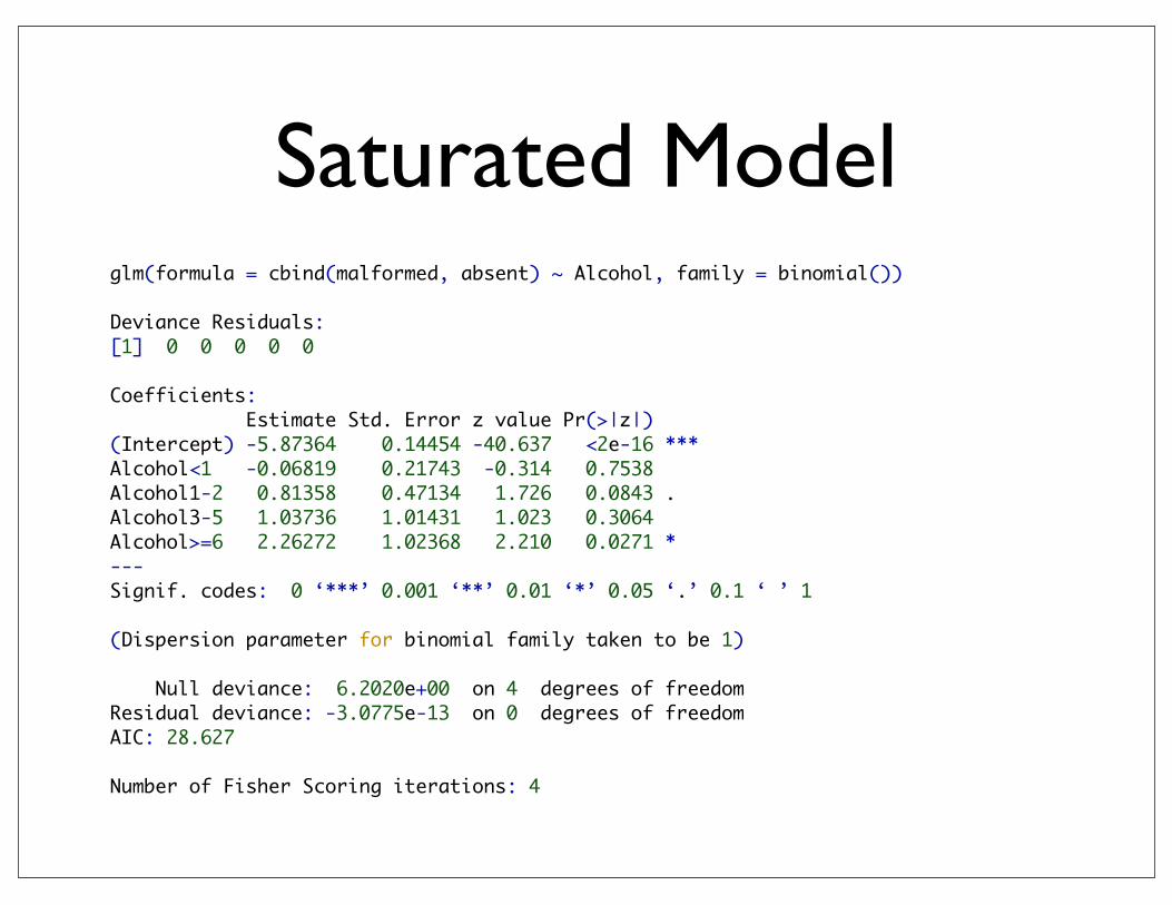
Saturated Modelglm(formula = cbind(malformed, absent) ~ Alcohol, family = binomial())

Deviance Residuals: [1] 0 0 0 0 0

Coefficients: Estimate Std. Error z value Pr(>|z|) (Intercept) -5.87364 0.14454 -40.637 <2e-16 ***Alcohol<1 -0.06819 0.21743 -0.314 0.7538 Alcohol1-2 0.81358 0.47134 1.726 0.0843 . Alcohol3-5 1.03736 1.01431 1.023 0.3064 Alcohol>=6 2.26272 1.02368 2.210 0.0271 * ---Signif. codes: 0 ‘***’ 0.001 ‘**’ 0.01 ‘*’ 0.05 ‘.’ 0.1 ‘ ’ 1

(Dispersion parameter for binomial family taken to be 1)

Null deviance: 6.2020e+00 on 4 degrees of freedomResidual deviance: -3.0775e-13 on 0 degrees of freedomAIC: 28.627

Number of Fisher Scoring iterations: 4

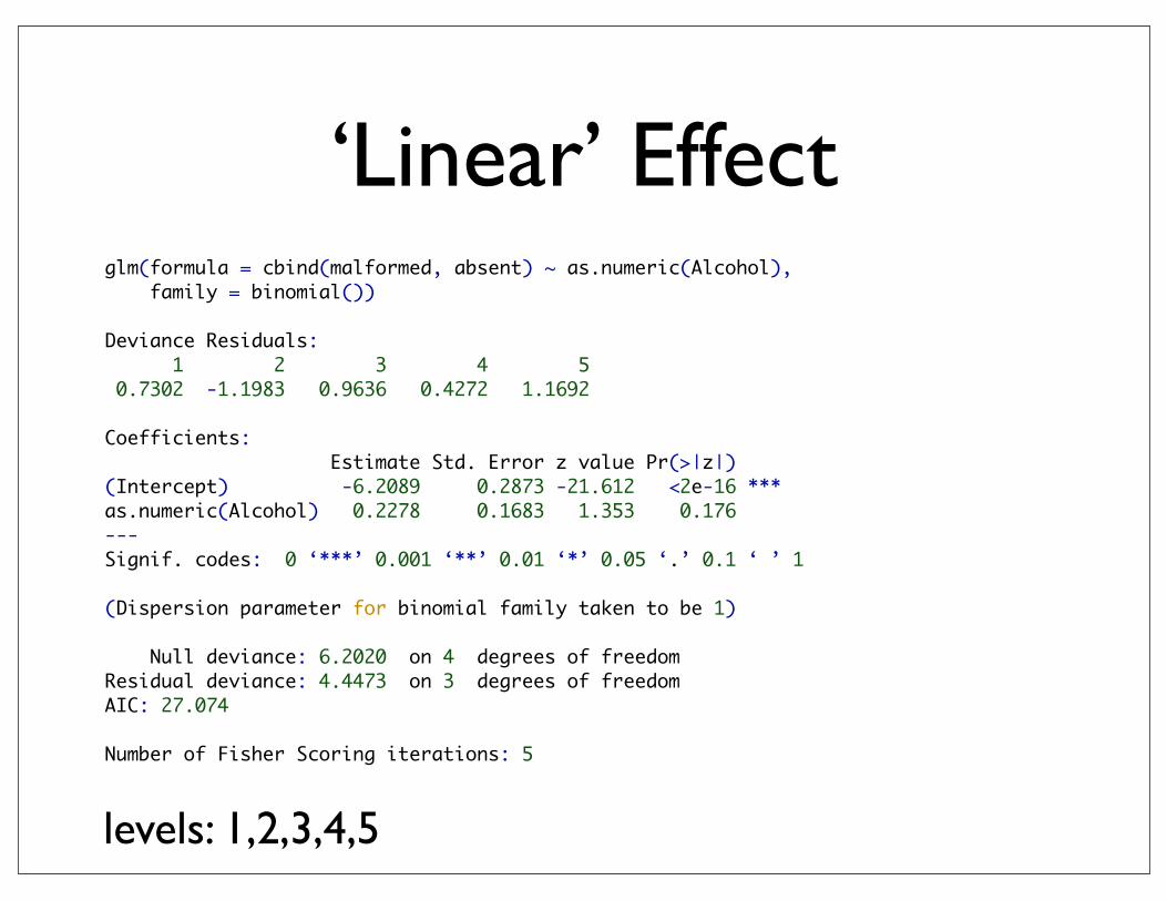
‘Linear’ Effectglm(formula = cbind(malformed, absent) ~ as.numeric(Alcohol), family = binomial())

Deviance Residuals: 1 2 3 4 5 0.7302 -1.1983 0.9636 0.4272 1.1692

Coefficients: Estimate Std. Error z value Pr(>|z|) (Intercept) -6.2089 0.2873 -21.612 <2e-16 ***as.numeric(Alcohol) 0.2278 0.1683 1.353 0.176 ---Signif. codes: 0 ‘***’ 0.001 ‘**’ 0.01 ‘*’ 0.05 ‘.’ 0.1 ‘ ’ 1


Null deviance: 6.2020 on 4 degrees of freedomResidual deviance: 4.4473 on 3 degrees of freedomAIC: 27.074


levels: 1,2,3,4,5

‘Linear’ Effectglm(formula = cbind(malformed, absent) ~ as.numeric(Alcohol), family = binomial())

Deviance Residuals: 1 2 3 4 5 0.5921 -0.8801 0.8865 -0.1449 0.1291

Coefficients: Estimate Std. Error z value Pr(>|z|) (Intercept) -5.9605 0.1154 -51.637 <2e-16 ***as.numeric(Alcohol) 0.3166 0.1254 2.523 0.0116 * ---Signif. codes: 0 ‘***’ 0.001 ‘**’ 0.01 ‘*’ 0.05 ‘.’ 0.1 ‘ ’ 1


Null deviance: 6.2020 on 4 degrees of freedomResidual deviance: 1.9487 on 3 degrees of freedomAIC: 24.576


levels: 0,0.5,1.5,4,7

Ordinal X

• Scores of categorical variables critically influence a model

• usually, scores will be given by data experts

• various choices: e.g. midpoints of interval variables,

• assume default scores are values 1 to n

• Linear changes to scores do not affect the overall model (predictions, goodness of fit)

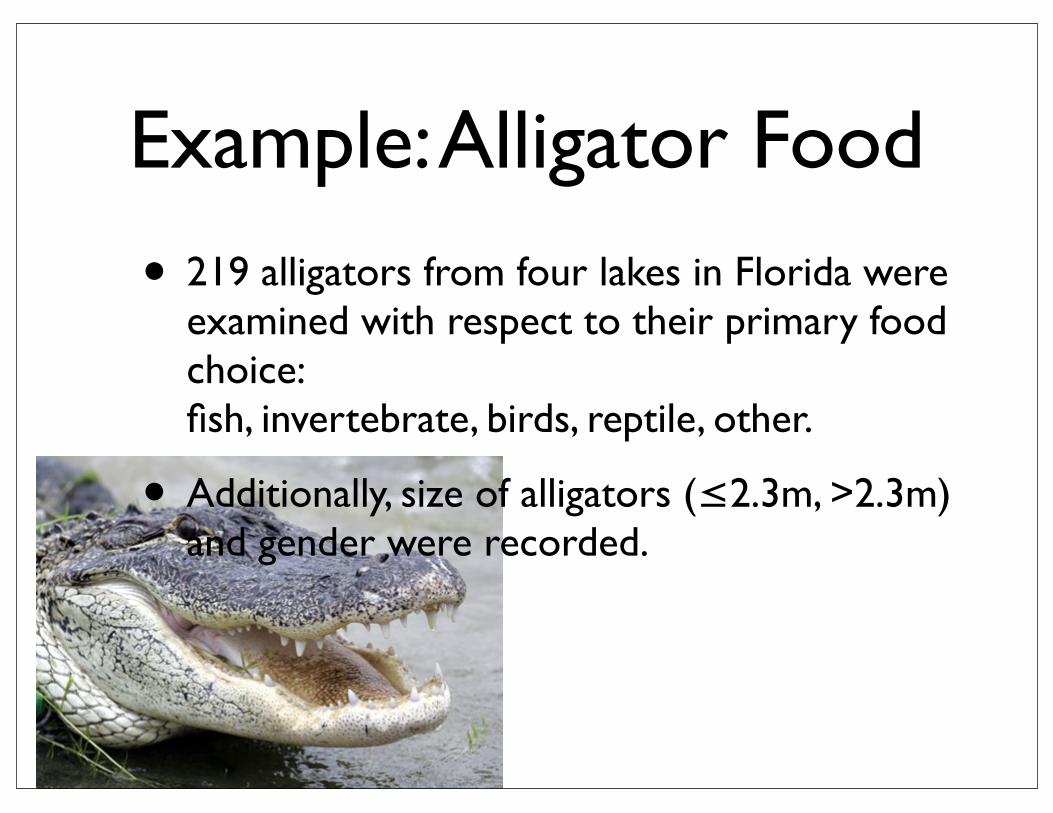
Example: Alligator Food

• 219 alligators from four lakes in Florida were examined with respect to their primary food choice: fish, invertebrate, birds, reptile, other.

• Additionally, size of alligators (≤2.3m, >2.3m) and gender were recorded.

> summary(alligator) ID food size gender lake Min. : 1.0 bird :13 <2.3:124 f: 89 george :63 1st Qu.: 55.5 fish :94 >2.3: 95 m:130 hancock :55 Median :110.0 invert:61 oklawaha:48 Mean :110.0 other :32 trafford:53 3rd Qu.:164.5 rep :19 Max. :219.0

fish

bird

invert

otherrep

> summary(alligator) ID food size gender lake Min. : 1.0 bird :13 <2.3:124 f: 89 george :63 1st Qu.: 55.5 fish :94 >2.3: 95 m:130 hancock :55 Median :110.0 invert:61 oklawaha:48 Mean :110.0 other :32 trafford:53 3rd Qu.:164.5 rep :19 Max. :219.0

Baseline Categorical Model

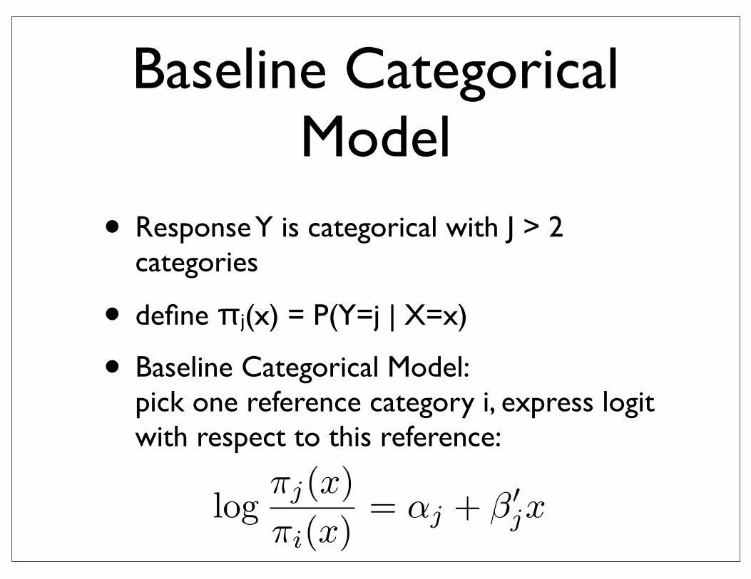
• Response Y is categorical with J > 2 categories

• define πj(x) = P(Y=j | X=x)

• Baseline Categorical Model: pick one reference category i, express logit with respect to this reference:

5 Logit Models for Multinomial Logit

Let response variable Y be a nominal variable with J > 2 categories.

5.1 Baseline Category Logit Models

Pick one “special” category i, e.g. i = 1 or i = J or i is largest category of Y . Then define

logπj(x)πi(x)

= αj + β�jx for all j = 1, ..., J and all x.

It is enough to just look at the J − 1 differences; for categories a and b we get a comparison by

logπa(x)πb(x)

= logπa(x)πi(x)

− logπb(x)πi(x)

= (αa − αb) + (βa − βb)�x.

Haberman : G2 and X2 are χ2 distributed, if data is categorical and not sparse; if data is sparse orcontinuous, deviance differences between nested models are still χ2 distributed, if the models differ in fewparameters.

Example: Alligator - Food Choice 219 alligators were examined with respect to their primary foodchoice (fish, invertebrae, birds, reptile, other). Explanatory variables are lake (4 categories), size( < 2.3m, >2.3m) and gender. The full model then has the form

logπj(x)πF (x)

= αj + βLlj + βS

sj + βGgj + βLS

lsj + βLGlgj + βSG

sgj + βLSGlsgj , for j = 1, ..., 4

the number of parameters we estimate is then (in the above order):

(1 + 3 + 1 + 1 + 3 + 3 + 1 + 3) · 4 = 16 · 4 = 64

The full model has 0 degrees of freedom:

> library(nnet)> options(contrasts=c("contr.treatment","contr.poly"))> fitS<-multinom(food~lake*size*gender,data=table.7.1) # saturated model# weights: 85 (64 variable)initial value 352.466903iter 10 value 261.200857iter 20 value 245.788420iter 30 value 244.090612iter 40 value 243.812122iter 50 value 243.801212final value 243.800899converged

Since we only have 219 observations on 80 cells, we deal with a sparse table problem. We are only able tocompare differences of deviances.

fit0<-multinom(food~1,data=table.7.1) # nullfit1<-multinom(food~gender,data=table.7.1) # Gfit2<-multinom(food~size,data=table.7.1) # Sfit3<-multinom(food~lake,data=table.7.1) # Lfit4<-multinom(food~size+lake,data=table.7.1) # L + S

58

Multinomial Model

• Choices for baseline:

• largest category gives most stable results

• R picks first level

• Haberman : G2 and X2 are χ2 distributed, if data is categorical and not sparse; for sparse or continuous data, deviance differences between nested models are still χ2 distributed, if the models differ in few parameters.

library(nnet)

• Brian Ripley’s nnet package allows to fit multinomial models:

library(nnet)alli.main <- multinom(food~lake+size+gender, data=alligator)

> summary(alli.main)Call:multinom(formula = food ~ lake + size + gender, data = alligator)

Coefficients: (Intercept) lakehancock lakeoklawaha laketrafford size>2.3bird -2.4321397 0.5754699 -0.55020075 1.237216 0.7300740invert 0.1690702 -1.7805555 0.91304120 1.155722 -1.3361658other -1.4309095 0.7667093 0.02603021 1.557820 -0.2905697rep -3.4161432 1.1296426 2.53024945 3.061087 0.5571846 gendermbird -0.6064035invert -0.4629388other -0.2524299rep -0.6276217

Std. Errors: (Intercept) lakehancock lakeoklawaha laketrafford size>2.3bird 0.7706720 0.7952303 1.2098680 0.8661052 0.6522657invert 0.3787475 0.6232075 0.4761068 0.4927795 0.4111827other 0.5381162 0.5685673 0.7777958 0.6256868 0.4599317rep 1.0851582 1.1928075 1.1221413 1.1297557 0.6466092 gendermbird 0.6888385invert 0.3955162other 0.4663546rep 0.6852750

Residual Deviance: 537.8655 AIC: 585.8655

Alligator

• Full Model has the form

• # parameters estimated:(1 + 3 + 1 + 1 + 3 + 3 + 1 + 3) * 4 = 64

• find suitable sub-model

5 Logit Models for Multinomial Logit

Let response variable Y be a nominal variable with J > 2 categories.

5.1 Baseline Category Logit Models

Pick one “special” category i, e.g. i = 1 or i = J or i is largest category of Y . Then define

logπj(x)πi(x)

= αj + β�jx for all j = 1, ..., J and all x.

It is enough to just look at the J − 1 differences; for categories a and b we get a comparison by

logπa(x)πb(x)

= logπa(x)πi(x)

− logπb(x)πi(x)

= (αa − αb) + (βa − βb)�x.

Haberman : G2 and X2 are χ2 distributed, if data is categorical and not sparse; if data is sparse orcontinuous, deviance differences between nested models are still χ2 distributed, if the models differ in fewparameters.

Example: Alligator - Food Choice 219 alligators were examined with respect to their primary foodchoice (fish, invertebrae, birds, reptile, other). Explanatory variables are lake (4 categories), size( < 2.3m, >2.3m) and gender. The full model then has the form

logπj(x)πF (x)

= αj + βLlj + βS

sj + βGgj + βLS

lsj + βLGlgj + βSG

sgj + βLSGlsgj , for j = 1, ..., 4

the number of parameters we estimate is then (in the above order):

(1 + 3 + 1 + 1 + 3 + 3 + 1 + 3) · 4 = 16 · 4 = 64

The full model has 0 degrees of freedom:

> library(nnet)> options(contrasts=c("contr.treatment","contr.poly"))> fitS<-multinom(food~lake*size*gender,data=table.7.1) # saturated model# weights: 85 (64 variable)initial value 352.466903iter 10 value 261.200857iter 20 value 245.788420iter 30 value 244.090612iter 40 value 243.812122iter 50 value 243.801212final value 243.800899converged

Since we only have 219 observations on 80 cells, we deal with a sparse table problem. We are only able tocompare differences of deviances.

fit0<-multinom(food~1,data=table.7.1) # nullfit1<-multinom(food~gender,data=table.7.1) # Gfit2<-multinom(food~size,data=table.7.1) # Sfit3<-multinom(food~lake,data=table.7.1) # Lfit4<-multinom(food~size+lake,data=table.7.1) # L + S

58

Alligator

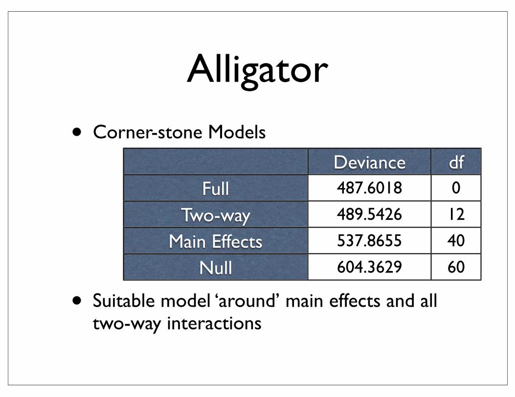
• Corner-stone Models

• Suitable model ‘around’ main effects and all two-way interactions

Deviance dfFull

Two-wayMain Effects

Null

487.6018 0

489.5426 12

537.8655 40

604.3629 60

> anova(alli.full, alli.twoway, alli.main, alli.null) Model Resid. df Resid. Dev1 1 872 604.36292 lake + size + gender 852 537.86553 size * gender * lake - size:gender:lake 824 489.54264 size * gender * lake 812 487.6018 Test Df LR stat. Pr(Chi)1 NA NA NA2 1 vs 2 20 66.497442 6.723394e-073 2 vs 3 28 48.322909 9.889238e-034 3 vs 4 12 1.940776 9.994914e-01

Estimated Response

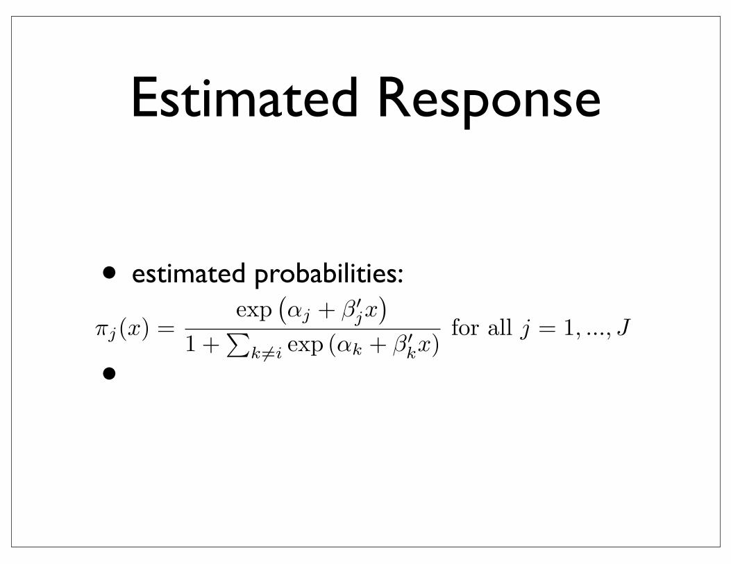
• estimated probabilities:

•

Estimated Response Probabilities For model

logπj(x)πi(x)

= αj + β�jx for all j = 1, ..., J and all x (1)

the estimated response probabilities are given as

πj(x) =exp

�αj + β�

jx�

1 +�

k �=i exp (αk + β�kx)

for all j = 1, ..., J

Proof:Because of the modeling assumption we have for all j = 1, ..., J :

logπj(x)πi(x)

= αj + β�jx

Thereforeπj(x)πi(x)

= exp�αj + β�

jx�

Since�

j πj(x) = 1, we have

1πi(x)

=�

j

πj(x)πi(x)

=�

j

exp�αj + β�

jx�

= 1 +�

j �=i

exp�αj + β�

jx�

With πi(x) =�1 +

�j �=i exp

�αj + β�

jx��−1

, we get

πj(x) =exp

�αj + β�

jx�

1 +�

j �=i exp�αj + β�

jx� .

Example: Alligator - Food Choice For the Alligator Data, the estimated probabilities for primary foodchoices are:

> predict(fitS,type="probs")[!duplicated(predict(fitS,type="probs")),]

fish invert rep bird otherhancock <2.3 0.5353 0.0931 0.0475 0.0704 0.2537hancock >2.3 0.5702 0.0231 0.0718 0.1409 0.1940oklawaha <2.3 0.2582 0.6019 0.0772 0.0088 0.0539oklawaha >2.3 0.4584 0.2486 0.1948 0.0294 0.0687trafford <2.3 0.1843 0.5168 0.0888 0.0359 0.1742trafford >2.3 0.2957 0.1930 0.2024 0.1082 0.2007george <2.3 0.4521 0.4128 0.0116 0.0297 0.0938george >2.3 0.6575 0.1397 0.0239 0.0810 0.0979

60

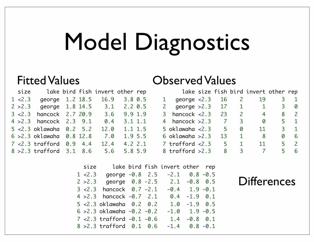
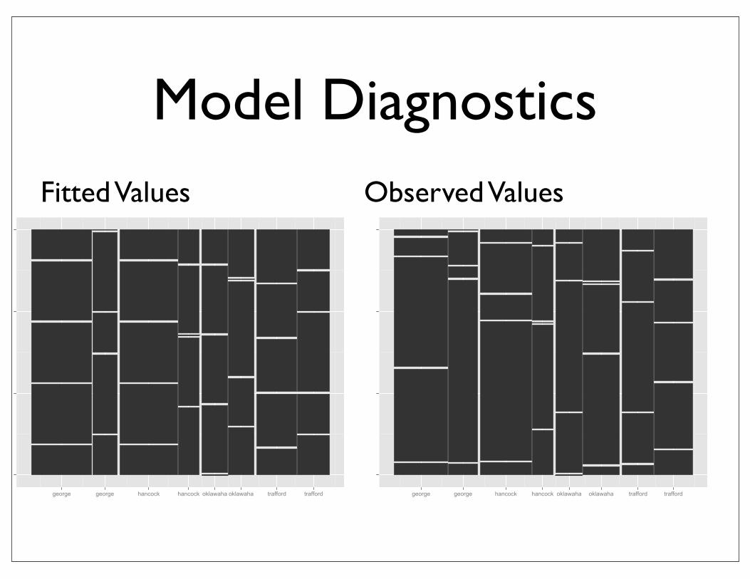
Model Diagnostics

size lake bird fish invert other rep1 <2.3 george 1.2 18.5 16.9 3.8 0.52 >2.3 george 1.8 14.5 3.1 2.2 0.53 <2.3 hancock 2.7 20.9 3.6 9.9 1.94 >2.3 hancock 2.3 9.1 0.4 3.1 1.15 <2.3 oklawaha 0.2 5.2 12.0 1.1 1.56 >2.3 oklawaha 0.8 12.8 7.0 1.9 5.57 <2.3 trafford 0.9 4.4 12.4 4.2 2.18 >2.3 trafford 3.1 8.6 5.6 5.8 5.9

Fitted Values lake size fish bird invert other rep1 george <2.3 16 2 19 3 12 george >2.3 17 1 1 3 03 hancock <2.3 23 2 4 8 24 hancock >2.3 7 3 0 5 15 oklawaha <2.3 5 0 11 3 16 oklawaha >2.3 13 1 8 0 67 trafford <2.3 5 1 11 5 28 trafford >2.3 8 3 7 5 6

Observed Values

size lake bird fish invert other rep1 <2.3 george -0.8 2.5 -2.1 0.8 -0.52 >2.3 george 0.8 -2.5 2.1 -0.8 0.53 <2.3 hancock 0.7 -2.1 -0.4 1.9 -0.14 >2.3 hancock -0.7 2.1 0.4 -1.9 0.15 <2.3 oklawaha 0.2 0.2 1.0 -1.9 0.56 >2.3 oklawaha -0.2 -0.2 -1.0 1.9 -0.57 <2.3 trafford -0.1 -0.6 1.4 -0.8 0.18 >2.3 trafford 0.1 0.6 -1.4 0.8 -0.1

Differences

Model Diagnostics



Observed Values

size lake bird fish invert other rep1 <2.3 george -0.6 0.1 -0.1 0.2 -1.12 >2.3 george 0.4 -0.2 0.7 -0.4 1.03 <2.3 hancock 0.3 -0.1 -0.1 0.2 -0.14 >2.3 hancock -0.3 0.2 1.0 -0.6 0.15 <2.3 oklawaha 1.0 0.0 0.1 -1.8 0.46 >2.3 oklawaha -0.2 0.0 -0.1 1.0 -0.17 <2.3 trafford -0.2 -0.1 0.1 -0.2 0.18 >2.3 trafford 0.0 0.1 -0.3 0.1 0.0

Pearson Residuals

Model Diagnostics



Observed Values

george george hancock hancock oklawaha oklawaha trafford trafford george george hancock hancock oklawaha oklawaha trafford trafford

Proportional Odds Logistic Regression

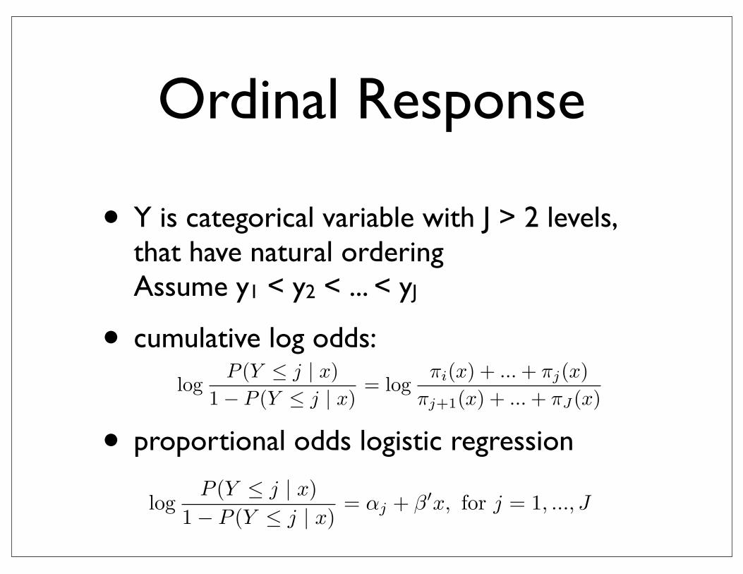
Ordinal Response

• Y is categorical variable with J > 2 levels, that have natural orderingAssume y1 < y2 < ... < yJ

• cumulative log odds:

• proportional odds logistic regression

Fitted data


Observed data

fish invert rep bird other23 4 2 2 87 0 1 3 55 11 1 0 313 8 6 1 05 11 2 1 58 7 6 3 516 19 1 2 317 1 0 1 3

Comparing observed and fitted cell counts gives an idea of the sign of the residuals. For a more precise

comparison we will use the same residuals as before, e.g. Pearsons residuals

oij − eij√eij

,

where we have asymptotic distributions.

5.2 Proportional Odds Model

If the response variable Y is ordinal, we can take a different approach to modeling it: based on the cumulative

probability P (Y ≤ j | x) for j = 1, ..., J we define the cumulative log odds as

logP (Y ≤ j | x)

1− P (Y ≤ j | x)= log

πi(x) + ... + πj(x)

πj+1(x) + ... + πJ(x)

The cumulative odds model or proportional odds model is then given as

logP (Y ≤ j | x)

1− P (Y ≤ j | x)= αj + β�x, for j = 1, ..., J

The values αj are ordered, i.e. αj1 ≤ αj2 for j1 < j2: for j1 < j2, the cumulative probabilities have

the same ordering: P (Y ≤ j1 | x) ≤ P (Y ≤ j2 | x). Since the logit is a monotone increasing function,

logit P (Y ≤ j1 | x) ≤ logit P (Y ≤ j2 | x). Using the above model hypothesis, this implies αj1 ≤ αj2 .

The curves for the estimated probabilities are shifts to the left for higher levels of Y , because for continuous

variable X and β �= 0:

logit P (Y ≤ j | x) = logit P (Y ≤ k | x− (αk − αj)/β),

since P (Y ≤ k | x− (αk −αj)/β) = αk + β · (x− (αk − αj)/β) = αk −αk + αj + βx, i.e. for j < k the curve

for P (Y ≤ k) is the same curve as for P (Y ≤ j translated by (αk − αj)/β units in direction X.m00M0M

0

22M2M

2

44M4M

4

66M6M

6

88M8M

8

1010M10M

10

m0.00.0M0.0M

0.0

0.20.2M0.2M

0.2

0.40.4M0.4M

0.4

0.60.6M0.6M

0.6

0.80.8M0.8M

0.8

1.01.0M1.0M

1.0

xMxM

x

Estimated ProbabilitiesMEstimated ProbabilitiesM

Estim

ate

d P

rob

ab

ilitie

s

P(Y 1)MP(Y 1)M

P(Y 1)

P(Y <= 1)MP(Y <= 1)M

P(Y <= 1)

P(Y <= 2)MP(Y <= 2)M

P(Y <= 2)

P(Y <= 3)MP(Y <= 3)M

P(Y <= 3)

61

Fitted data


Observed data

fish invert rep bird other23 4 2 2 87 0 1 3 55 11 1 0 313 8 6 1 05 11 2 1 58 7 6 3 516 19 1 2 317 1 0 1 3

Comparing observed and fitted cell counts gives an idea of the sign of the residuals. For a more precise

comparison we will use the same residuals as before, e.g. Pearsons residuals

oij − eij√eij

,

where we have asymptotic distributions.

5.2 Proportional Odds Model

If the response variable Y is ordinal, we can take a different approach to modeling it: based on the cumulative

probability P (Y ≤ j | x) for j = 1, ..., J we define the cumulative log odds as

logP (Y ≤ j | x)

1− P (Y ≤ j | x)= log

πi(x) + ... + πj(x)

πj+1(x) + ... + πJ(x)

The cumulative odds model or proportional odds model is then given as

logP (Y ≤ j | x)

1− P (Y ≤ j | x)= αj + β�x, for j = 1, ..., J

The values αj are ordered, i.e. αj1 ≤ αj2 for j1 < j2: for j1 < j2, the cumulative probabilities have

the same ordering: P (Y ≤ j1 | x) ≤ P (Y ≤ j2 | x). Since the logit is a monotone increasing function,

logit P (Y ≤ j1 | x) ≤ logit P (Y ≤ j2 | x). Using the above model hypothesis, this implies αj1 ≤ αj2 .

The curves for the estimated probabilities are shifts to the left for higher levels of Y , because for continuous

variable X and β �= 0:

logit P (Y ≤ j | x) = logit P (Y ≤ k | x− (αk − αj)/β),

since P (Y ≤ k | x− (αk −αj)/β) = αk + β · (x− (αk − αj)/β) = αk −αk + αj + βx, i.e. for j < k the curve

for P (Y ≤ k) is the same curve as for P (Y ≤ j translated by (αk − αj)/β units in direction X.m00M0M

0

22M2M

2

44M4M

4

66M6M

6

88M8M

8

1010M10M

10

m0.00.0M0.0M

0.0

0.20.2M0.2M

0.2

0.40.4M0.4M

0.4

0.60.6M0.6M

0.6

0.80.8M0.8M

0.8

1.01.0M1.0M

1.0

xMxM

x

Estimated ProbabilitiesMEstimated ProbabilitiesM

Estim

ate

d P

rob

ab

ilitie

s

P(Y 1)MP(Y 1)M

P(Y 1)

P(Y <= 1)MP(Y <= 1)M

P(Y <= 1)

P(Y <= 2)MP(Y <= 2)M

P(Y <= 2)

P(Y <= 3)MP(Y <= 3)M

P(Y <= 3)

61

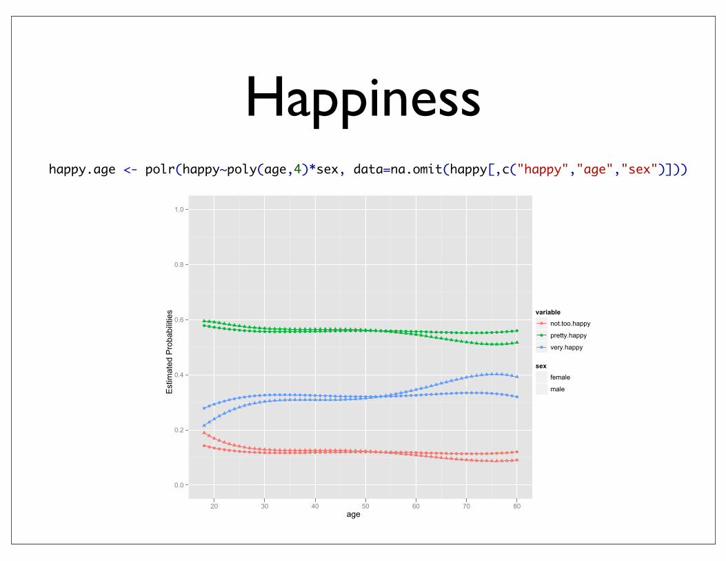
Happiness

age

Estim

ate

d P

robabilitie

s

0.0

0.2

0.4

0.6

0.8

1.0

20 30 40 50 60 70 80

variable

not.too.happy

pretty.happy

very.happy

sex

female

male

happy.age <- polr(happy~poly(age,4)*sex, data=na.omit(happy[,c("happy","age","sex")]))

multinomial logistic regression - nutritionista · 5 logit models for multinomial logit let...

Documents