multifaceted feature visualization: uncovering the ...multifaceted feature visualization: uncovering...

Multifaceted Feature Visualization: Uncovering the Different Types of FeaturesLearned By Each Neuron in Deep Neural Networks

Anh Nguyen [email protected]

University of Wyoming

Jason Yosinski [email protected]

Cornell University

Jeff Clune [email protected]

University of Wyoming

Abstract

We can better understand deep neural networksby identifying which features each of their neu-rons have learned to detect. To do so, researchershave created Deep Visualization techniques in-cluding activation maximization, which synthet-ically generates inputs (e.g. images) that maxi-mally activate each neuron. A limitation of cur-rent techniques is that they assume each neurondetects only one type of feature, but we knowthat neurons can be multifaceted, in that theyfire in response to many different types of fea-tures: for example, a grocery store class neuronmust activate either for rows of produce or fora storefront. Previous activation maximizationtechniques constructed images without regard forthe multiple different facets of a neuron, creatinginappropriate mixes of colors, parts of objects,scales, orientations, etc. Here, we introduce analgorithm that explicitly uncovers the multiplefacets of each neuron by producing a syntheticvisualization of each of the types of images thatactivate a neuron. We also introduce regular-ization methods that produce state-of-the-art re-sults in terms of the interpretability of imagesobtained by activation maximization. By sepa-rately synthesizing each type of image a neuronfires in response to, the visualizations have moreappropriate colors and coherent global structure.Multifaceted feature visualization thus providesa clearer and more comprehensive description ofthe role of each neuron.

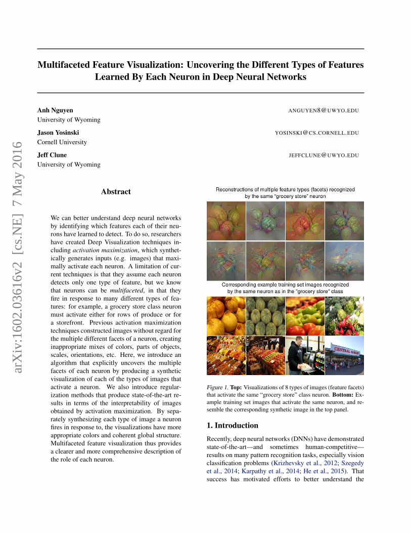
Figure 1. Top: Visualizations of 8 types of images (feature facets)that activate the same “grocery store” class neuron. Bottom: Ex-ample training set images that activate the same neuron, and re-semble the corresponding synthetic image in the top panel.

1. IntroductionRecently, deep neural networks (DNNs) have demonstratedstate-of-the-art—and sometimes human-competitive—results on many pattern recognition tasks, especially visionclassification problems (Krizhevsky et al., 2012; Szegedyet al., 2014; Karpathy et al., 2014; He et al., 2015). Thatsuccess has motivated efforts to better understand the

arX

iv:1

602.

0361

6v2

[cs

.NE

] 7

May

201

6

Multifaceted Feature Visualization

inner workings of such networks, which enables us tofurther improve their architectures, learning algorithms,and hyperparameters. An active area of research in thisvein, called Deep Visualization, involves taking a trainedDNN and creating synthetic images that produce specificneural activations of interest within it (Zeiler et al., 2014;Yosinski et al., 2015; Karpathy et al., 2015; Dosovitskiyet al., 2015; Mahendran et al., 2015; Nguyen et al., 2015;Bach et al., 2015a; Simonyan et al., 2013; Wei et al., 2015).

There are two general camps within Deep Visualization:activation maximization (Erhan et al., 2009) and code in-version (Mahendran et al., 2015). Activation maximizationis the task of finding an image that maximally activates acertain neuron (aka “unit”, “feature”, or “feature detector”),which can reveal what each neuron in a DNN has learned tofire in response to (i.e. which features it detects). This tech-nique can be performed for the output neurons, such as neu-rons that classify types of images (Simonyan et al., 2013),and can also be performed for each of the hidden neuronsin a DNN (Erhan et al., 2009; Yosinski et al., 2015). Codeinversion is the problem of synthesizing an image that, fora specific DNN layer, produces a similar activation vectorat that layer as a target activation vector produced by a spe-cific real image (Mahendran et al., 2015; Dosovitskiy et al.,2015). It reveals what information about one specific imageis encoded by the DNN code at a particular layer.

Both activation maximization and code inversion start froma random image and calculate via backpropagation how thecolor of each pixel should be changed to either increasethe activation of a neuron (for activation maximization) orproduce a layer code closer to the target (for code inver-sion). However, previous studies have shown that doing sousing only the gradient information produces unrealistic-looking images that are not recognizable (Simonyan et al.,2013; Nguyen et al., 2015), because the set of all possi-ble images is so vast that it is possible to produce imagesthat satisfy the objective, but are still unrecognizable. In-stead, we must both satisfy the objective and try to limitthe set of images to those that resemble natural images. Bi-asing optimization to produce more natural images can beaccomplished by incorporating natural image priors intooptimization, which has been shown to substantially im-prove the recognizability of the images generated (Mahen-dran et al., 2015; Yosinski et al., 2015). Many regulariza-tion techniques have been introduced that improve imagequality such as: Gaussian blur (Yosinski et al., 2015), α-norm (Simonyan et al., 2013), total variation (Mahendranet al., 2015), jitter (Mordvintsev et al., 2015), and data-driven patch priors (Wei et al., 2015).

While these techniques have improved Deep Visualizationmethods over the last two years, the resultant images pro-vide room for improvement: (1) the color distribution is

unnatural (Fig. 8b-e); (2) recognizable fragments of imagesare repeated, but these fragments do not fit together into acoherent whole: e.g. multiple ostrich heads without bodies,or eyes without faces (Fig. 8b) (Simonyan et al., 2013; Ma-hendran et al., 2015); (3) previous techniques have no sys-tematic methods to visualize different facets (types of stim-uli) that a neuron responds to, but high-level neurons areknown to be multifaceted. For example, a face-detectingneuron in a DNN was shown to respond to both humanand lion faces (Yosinski et al., 2015). Neurons in humanbrains are similarly multifaceted: a “Halle Berry” neuronwas found that responds to very different stimuli related tothe actress, from pictures of her in costume to her nameprinted as text (Quiroga et al., 2005).

We name the class of algorithms that visualize differ-ent facets of a neuron multifaceted feature visualization(MFV). Erhan et al., 2009 found that optimizing an imageto maximally activate a neuron from multiple random start-ing images usually yielded the same final visualization. Incontrast, Wei et al., 2015 found that if the backpropagationneural pathway is masked out in a certain way, the resultantimages can sometimes reveal different feature facets. Thisis the first MFV method to our knowledge; however, it wasshown to visualize only two facets per output neuron, andis not able to systematically visualize all facets per neuron.

In this paper, we propose two Deep Visualization tech-niques. Most importantly, we introduce a novel MFV al-gorithm that:

1. Sheds much more light on the inner workings of DNNsthan other state-of-the-art Deep Visualization methodsby revealing the different facets of each neuron. It alsoreveals that neurons at all levels are multifaceted, andshows that higher-level neurons are more multifacetedthan lower-level ones (Fig. 6).

2. Improves the quality of synthesized images, producingstate-of-the-art activation maximization results: the col-ors are more natural and the images are more glob-ally consistent (Fig. 7. See also Figs. 1, 3, 4) becauseeach facet is separately synthesized. For example, MFVmakes one image of a green bell pepper and another of ared bell pepper instead of trying to simultaneously makeboth (Fig. 4). The increased global structure and con-textual details in the optimized images also support re-cent observations (Yosinski et al., 2015) that discrimina-tive DNNs encode not only knowledge of a sparse set ofdiscriminative features for performing classification, butalso more holistic information about typical input exam-ples in a manner more reminiscent of generative models.

3. Is simple to implement. The only main difference is howactivation maximization algorithms are initialized. Toobtain an initialization per facet, we project the training


set images that maximally activate a neuron into a low-dimensional space (here, a 2D space via t-SNE), clusterthe images via k-means, and average the n (here, 15)closest images to each cluster centroid to produce theinitial image (Section 3).

We also introduce a center-biased regularization techniquethat attempts to produce one central object. It combats aflaw with all activation maximization techniques includingMFV: they tend to produce many repeated object fragmentsin an image, instead of objects with more coherent globalstructure. It does so by allowing, on average, more opti-mization iterations for center pixels than edge pixels.

2. Methods2.1. Convolutional neural networks

For comparison with recent studies, we test our DeepVisualization methods on a variant of the well-known“AlexNet” convnet architecture (Krizhevsky et al., 2012),which is trained on the 1.3-million-image ILSVRC 2012ImageNet dataset (Deng et al., 2009; Russakovsky et al.,2014). Specifically, our DNN follows the CaffeNet ar-chitecture (Jia et al., 2014) with the weights providedby Yosinski et al., 2015. While this network is slightly dif-ferent than AlexNet, the changes are inconsequential: thenetwork obtains a 20.1% top-5 error rate, which is similarto AlexNet’s 18.2% (Krizhevsky et al., 2012).

The last three layers of the DNN are fully connected: wecall them fc6, fc7 and fc8. fc8 is the last layer (before soft-max transformation) and has 1000 outputs, one for eachImageNet class. fc6 and fc7 both have 4096 outputs.

2.2. Activation maximization

Informally, we run an optimization algorithm that opti-mizes the colors of the pixels in the image to maximallyactivate a particular neuron. That is accomplished by cal-culating the derivative of the target neuron activation withrespect to each pixel, which describes how to change thepixel color to increase the activation of that neuron. Wealso need to incorporate natural image priors to bias theimages to remain in the set of images that look as much aspossible like natural (i.e. real-world) images.

Formally, we may pose the activation maximization prob-lem for a unit with index j on a layer l of a network Φ asfinding an image x∗ where:

x∗ = arg maxx

(Φl,j(x)−Rθ(x)) (1)

Here, Rθ(x) is a parameterized regularization function thatcould include multiple regularizers (i.e. priors), each ofwhich penalizes the search in a different way to collec-

tively improve the image quality. We apply two regular-izers: total variation (TV) and jitter, as described in Ma-hendran et al. (2015), but via a slightly different, but qual-itatively similar, implementation. Supplementary Sec. S2details the differences and analyzes the benefits of incor-porating different regularizers used in previous activationmaximization papers: Gaussian blur (Yosinski et al., 2015),α-norm (Simonyan et al., 2013), total variation (TV) (Ma-hendran et al., 2015), jitter (Mordvintsev et al., 2015), and adata-driven patch prior (Wei et al., 2015). Our code and pa-rameters are available at http://EvolvingAI.org.

2.3. Multifaceted feature visualization

Although DNN feature detectors must recognize that verydifferent types of images all represent the same concept(e.g. a bell pepper detector must recognize green, red, andorange peppers as in the same class), there is no systematicmethod for visualizing these different facets of feature de-tectors. In this section, we introduce a method for visualiz-ing the multiple facets that each neuron in a DNN respondsto. We demonstrate the technique on the ImageNet dataset,although the results generalize beyond computer vision toany domain (e.g. speech recognition, machine translation).

We start with the observation that in the training set, eachImageNet class has multiple intra-class clusters that reflectdifferent facets of the class. For example, in the bell pep-per class, one finds bell peppers of different colors, aloneor in groups, cut open or whole, etc. (Fig. 4). We hypothe-sized that activation maximization on the bell pepper classis made difficult because which facet of the bell pepper tobe reconstructed is not specified, potentially meaning thatdifferent areas of the image may optimize toward recon-structing different fragments of different facets. We furtherhypothesized that if we initialize activation maximizationoptimization with the mean image of only one facet, thatmay increase the likelihood that optimization would recon-struct an image of that type. We also hypothesized thatwe can get reconstructions of different facets by startingoptimization with mean images from different facets. Ourexperimental results support all of these hypotheses.

Specifically, to visualize different facets of an output neu-ron C (e.g. the fc8 neuron that declares an image to be amember of the “bell pepper” class), we take all (∼1300)training set examples from that class and follow Algo-rithm 1 to produce k = 10 facet visualizations. Note that,here, we demonstrate the algorithm on the training set, andthe results are shown in Figs. 1, 3, 4 & 7. However, wealso apply the same technique on the validation set (seeSec. 3.2), and show its results in Fig. 6.

Intuitively, the idea is to (1) use a DNN’s learned, abstract,knowledge of images to determine the different types ofimages that activate a neuron, and then (2) initialize a state-

http://EvolvingAI.org


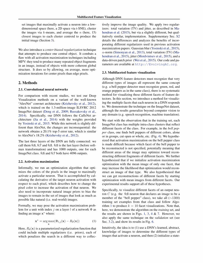
Algorithm 1 Multifaceted Feature Visualization

Input: a set of images U and a number of facets k1. for each image in U , compute high-level (here fc7)hidden code Φi2. Reduce the dimensionality of each code Φi from 4096to 50 via PCA.3. Run t-SNE visualization on the entire set of codes Φito produce a 2-D embedding (examples in Fig. 4).4. Locate k clusters in the embedding via k-means.for each cluster

5. Compute a mean image x0 by averaging the 15images nearest to the cluster centroid.6. Run activation maximization (see Section 2.2), butinitialize it with x0 instead of a random image.

Output: a set of facet visualizations {x1,x2, ...,xk}.

of-the-art activation maximization optimization algorithmwith the mean image computed from each of these clustersto visualize each facet. For (1), we first embed all of theimages in a class in a two-dimensional space via PCA (Per-son, 1901; Jolliffe, 2002) and t-SNE (Van der Maaten et al.,2008), and then perform k-means clustering (MacQueenet al., 1967) to find k types of images (Fig. 4). Notethat here we only visualize 10 facets per neuron, but itis possible to visualize fewer or more facets by changingk. We compute a mean image by averaging m = 15 im-ages (Algorithm 1, step 5) as it works the best compared tom = {1, 50, 100, 200} (data not shown). SupplementarySections S1 & S2.4 provide more intuition regarding whyinitializing from mean images helps.

2.4. Center-biased regularization

In activation maximization, to increase the activation of agiven neuron (e.g. an “ostrich” neuron), each “drawing”step often includes two types of updates: (1) intensifyingthe colors of existing ostriches in the image, and (2) draw-ing new fragments of ostriches (e.g. multiple heads). Sinceboth types of updates are non-separably encoded in the gra-dient, the results of previous activation maximization meth-ods are often images with many repeated image fragments(Fig. 8b-h). To ameliorate this issue, we introduce a tech-nique called center-biased regularization.

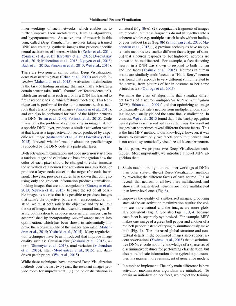
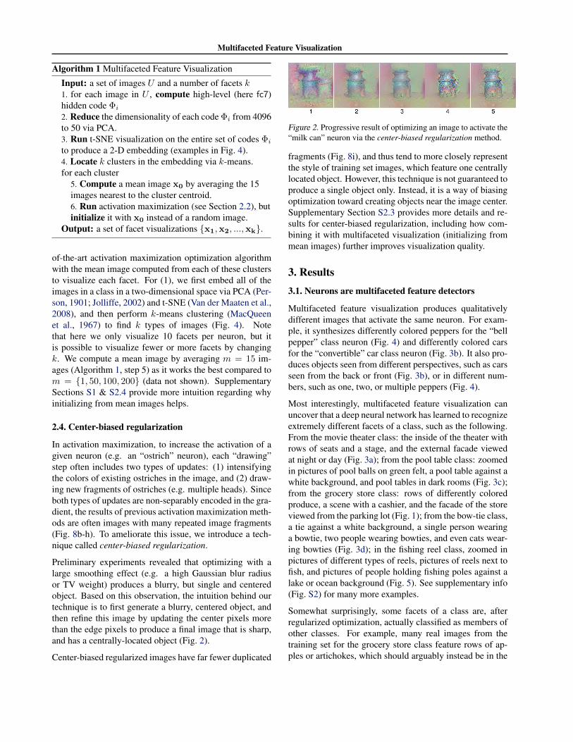
Preliminary experiments revealed that optimizing with alarge smoothing effect (e.g. a high Gaussian blur radiusor TV weight) produces a blurry, but single and centeredobject. Based on this observation, the intuition behind ourtechnique is to first generate a blurry, centered object, andthen refine this image by updating the center pixels morethan the edge pixels to produce a final image that is sharp,and has a centrally-located object (Fig. 2).

Center-biased regularized images have far fewer duplicated

Figure 2. Progressive result of optimizing an image to activate the“milk can” neuron via the center-biased regularization method.

fragments (Fig. 8i), and thus tend to more closely representthe style of training set images, which feature one centrallylocated object. However, this technique is not guaranteed toproduce a single object only. Instead, it is a way of biasingoptimization toward creating objects near the image center.Supplementary Section S2.3 provides more details and re-sults for center-biased regularization, including how com-bining it with multifaceted visualization (initializing frommean images) further improves visualization quality.

3. Results3.1. Neurons are multifaceted feature detectors

Multifaceted feature visualization produces qualitativelydifferent images that activate the same neuron. For exam-ple, it synthesizes differently colored peppers for the “bellpepper” class neuron (Fig. 4) and differently colored carsfor the “convertible” car class neuron (Fig. 3b). It also pro-duces objects seen from different perspectives, such as carsseen from the back or front (Fig. 3b), or in different num-bers, such as one, two, or multiple peppers (Fig. 4).

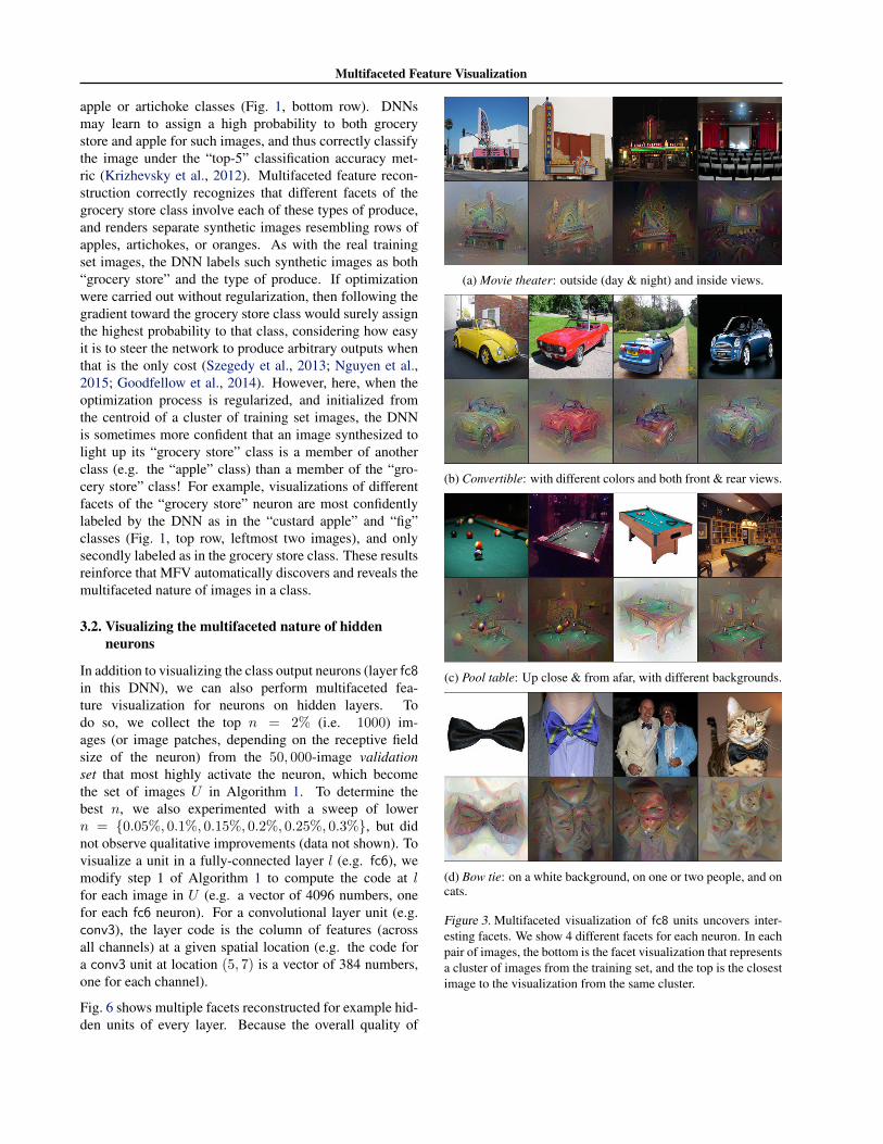
Most interestingly, multifaceted feature visualization canuncover that a deep neural network has learned to recognizeextremely different facets of a class, such as the following.From the movie theater class: the inside of the theater withrows of seats and a stage, and the external facade viewedat night or day (Fig. 3a); from the pool table class: zoomedin pictures of pool balls on green felt, a pool table against awhite background, and pool tables in dark rooms (Fig. 3c);from the grocery store class: rows of differently coloredproduce, a scene with a cashier, and the facade of the storeviewed from the parking lot (Fig. 1); from the bow-tie class,a tie against a white background, a single person wearinga bowtie, two people wearing bowties, and even cats wear-ing bowties (Fig. 3d); in the fishing reel class, zoomed inpictures of different types of reels, pictures of reels next tofish, and pictures of people holding fishing poles against alake or ocean background (Fig. 5). See supplementary info(Fig. S2) for many more examples.

Somewhat surprisingly, some facets of a class are, afterregularized optimization, actually classified as members ofother classes. For example, many real images from thetraining set for the grocery store class feature rows of ap-ples or artichokes, which should arguably instead be in the


apple or artichoke classes (Fig. 1, bottom row). DNNsmay learn to assign a high probability to both grocerystore and apple for such images, and thus correctly classifythe image under the “top-5” classification accuracy met-ric (Krizhevsky et al., 2012). Multifaceted feature recon-struction correctly recognizes that different facets of thegrocery store class involve each of these types of produce,and renders separate synthetic images resembling rows ofapples, artichokes, or oranges. As with the real trainingset images, the DNN labels such synthetic images as both“grocery store” and the type of produce. If optimizationwere carried out without regularization, then following thegradient toward the grocery store class would surely assignthe highest probability to that class, considering how easyit is to steer the network to produce arbitrary outputs whenthat is the only cost (Szegedy et al., 2013; Nguyen et al.,2015; Goodfellow et al., 2014). However, here, when theoptimization process is regularized, and initialized fromthe centroid of a cluster of training set images, the DNNis sometimes more confident that an image synthesized tolight up its “grocery store” class is a member of anotherclass (e.g. the “apple” class) than a member of the “gro-cery store” class! For example, visualizations of differentfacets of the “grocery store” neuron are most confidentlylabeled by the DNN as in the “custard apple” and “fig”classes (Fig. 1, top row, leftmost two images), and onlysecondly labeled as in the grocery store class. These resultsreinforce that MFV automatically discovers and reveals themultifaceted nature of images in a class.

3.2. Visualizing the multifaceted nature of hiddenneurons

In addition to visualizing the class output neurons (layer fc8in this DNN), we can also perform multifaceted fea-ture visualization for neurons on hidden layers. Todo so, we collect the top n = 2% (i.e. 1000) im-ages (or image patches, depending on the receptive fieldsize of the neuron) from the 50, 000-image validationset that most highly activate the neuron, which becomethe set of images U in Algorithm 1. To determine thebest n, we also experimented with a sweep of lowern = {0.05%, 0.1%, 0.15%, 0.2%, 0.25%, 0.3%}, but didnot observe qualitative improvements (data not shown). Tovisualize a unit in a fully-connected layer l (e.g. fc6), wemodify step 1 of Algorithm 1 to compute the code at lfor each image in U (e.g. a vector of 4096 numbers, onefor each fc6 neuron). For a convolutional layer unit (e.g.conv3), the layer code is the column of features (acrossall channels) at a given spatial location (e.g. the code fora conv3 unit at location (5, 7) is a vector of 384 numbers,one for each channel).

Fig. 6 shows multiple facets reconstructed for example hid-den units of every layer. Because the overall quality of

(a) Movie theater: outside (day & night) and inside views.

(b) Convertible: with different colors and both front & rear views.

(c) Pool table: Up close & from afar, with different backgrounds.

(d) Bow tie: on a white background, on one or two people, and oncats.

Figure 3. Multifaceted visualization of fc8 units uncovers inter-esting facets. We show 4 different facets for each neuron. In eachpair of images, the bottom is the facet visualization that representsa cluster of images from the training set, and the top is the closestimage to the visualization from the same cluster.


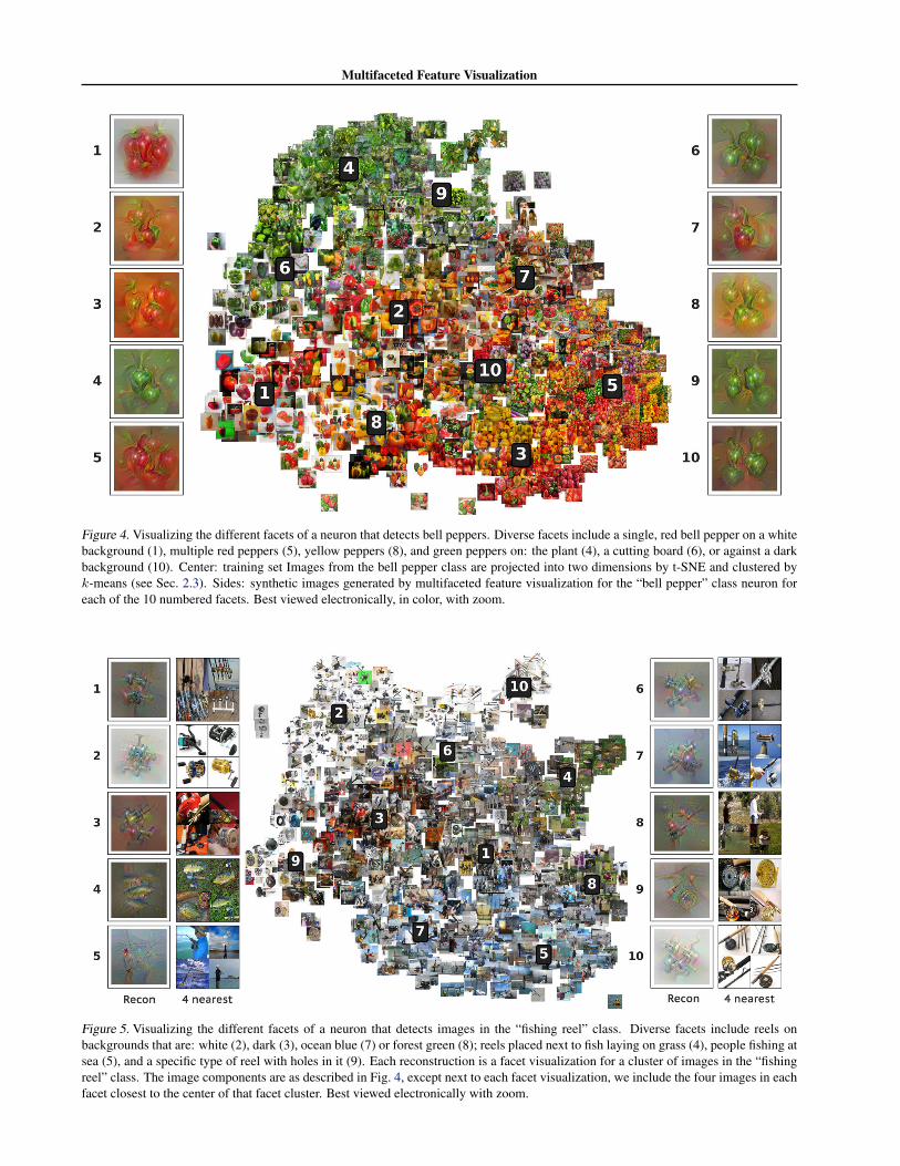
Figure 4. Visualizing the different facets of a neuron that detects bell peppers. Diverse facets include a single, red bell pepper on a whitebackground (1), multiple red peppers (5), yellow peppers (8), and green peppers on: the plant (4), a cutting board (6), or against a darkbackground (10). Center: training set Images from the bell pepper class are projected into two dimensions by t-SNE and clustered byk-means (see Sec. 2.3). Sides: synthetic images generated by multifaceted feature visualization for the “bell pepper” class neuron foreach of the 10 numbered facets. Best viewed electronically, in color, with zoom.

Figure 5. Visualizing the different facets of a neuron that detects images in the “fishing reel” class. Diverse facets include reels onbackgrounds that are: white (2), dark (3), ocean blue (7) or forest green (8); reels placed next to fish laying on grass (4), people fishing atsea (5), and a specific type of reel with holes in it (9). Each reconstruction is a facet visualization for a cluster of images in the “fishingreel” class. The image components are as described in Fig. 4, except next to each facet visualization, we include the four images in eachfacet closest to the center of that facet cluster. Best viewed electronically with zoom.


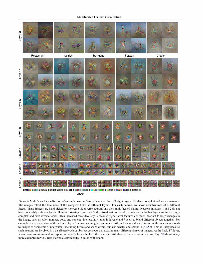
Figure 6. Multifaceted visualization of example neuron feature detectors from all eight layers of a deep convolutional neural network.The images reflect the true sizes of the receptive fields at different layers. For each neuron, we show visualizations of 4 differentfacets. These images are hand picked to showcase the diverse neurons and their multifaceted nature. Neurons in layers 1 and 2 do nothave noticeably different facets. However, starting from layer 3, the visualizations reveal that neurons at higher layers are increasinglycomplex and have diverse facets. This increased facet diversity is because higher level features are more invariant to large changes inthe image, such as color, number, pose, and context. Interestingly, units in layer 6 and 7 seem to blend different objects together. Forexample, the visualization of the leftmost layer 6 neuron seemingly combines a turtle and a scuba diver. It turns out this neuron respondsto images of “something underwater”, including turtles and scuba divers, but also whales and sharks (Fig. S5c). This is likely becausesuch neurons are involved in a distributed code of abstract concepts that exist in many different classes of images. At the final, 8th, layer,where neurons are trained to respond separately for each class, the facets are still diverse, but are within a class. Fig. S2 shows manymore examples for fc8. Best viewed electronically, in color, with zoom.


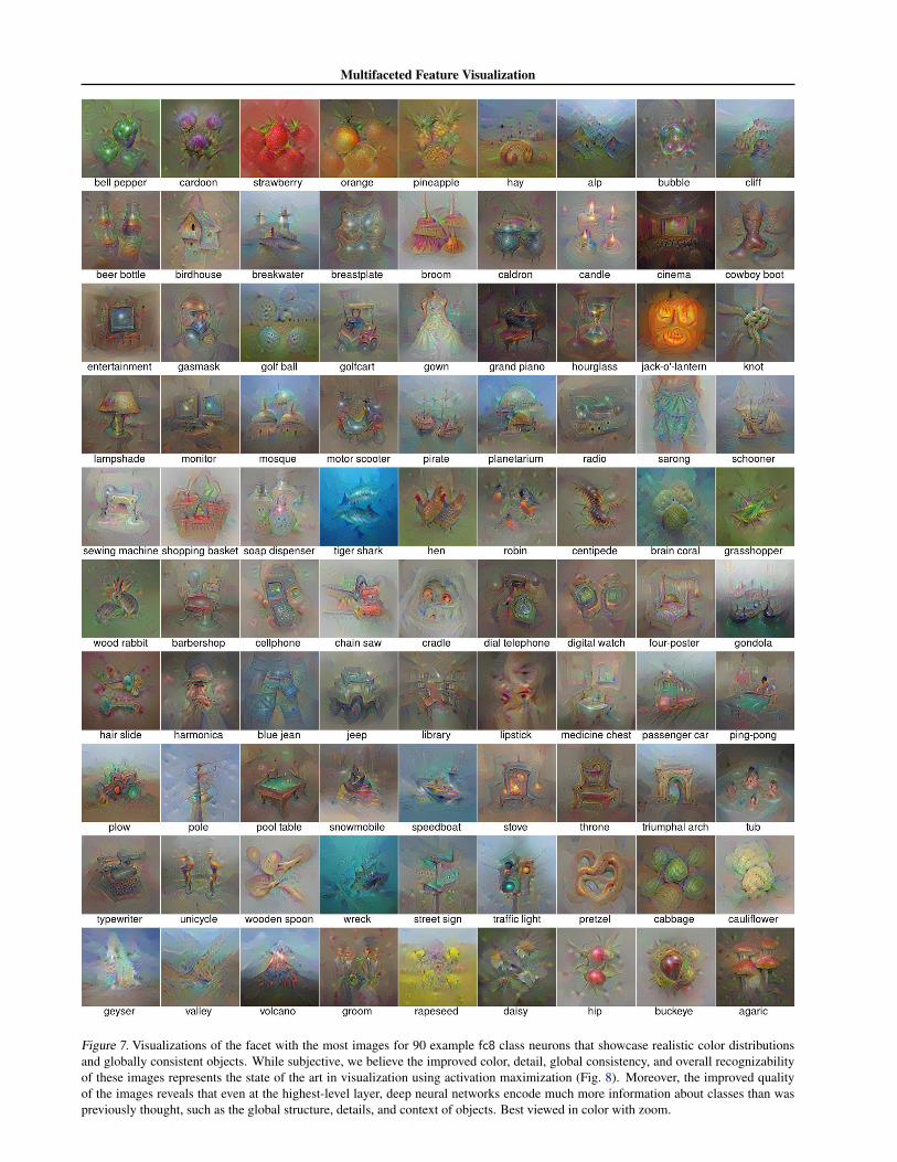
Figure 7. Visualizations of the facet with the most images for 90 example fc8 class neurons that showcase realistic color distributionsand globally consistent objects. While subjective, we believe the improved color, detail, global consistency, and overall recognizabilityof these images represents the state of the art in visualization using activation maximization (Fig. 8). Moreover, the improved qualityof the images reveals that even at the highest-level layer, deep neural networks encode much more information about classes than waspreviously thought, such as the global structure, details, and context of objects. Best viewed in color with zoom.


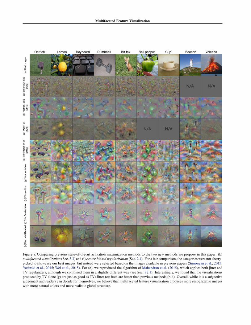
Figure 8. Comparing previous state-of-the-art activation maximization methods to the two new methods we propose in this paper: (k)multifaceted visualization (Sec. 3.3) and (i) center-biased regularization (Sec. 2.4). For a fair comparison, the categories were not cherry-picked to showcase our best images, but instead were selected based on the images available in previous papers (Simonyan et al., 2013;Yosinski et al., 2015; Wei et al., 2015). For (e), we reproduced the algorithm of Mahendran et al. (2015), which applies both jitter andTV regularizers, although we combined them in a slightly different way (see Sec. S2.1). Interestingly, we found that the visualizationsproduced by TV alone (g) are just as good as TV+Jitter (e); both are better than previous methods (b-d). Overall, while it is a subjectivejudgement and readers can decide for themselves, we believe that multifaceted feature visualization produces more recognizable imageswith more natural colors and more realistic global structure.


these visualizations is improved (discussed more below),it becomes easier to learn what each of these hidden neu-rons detects. Low-level layers (e.g. conv1 and conv2)do not exhibit noticeably different facets. However, start-ing at conv3, the qualitative difference between facets in-creases: first in slight differences of rotation, pose, andcolor, then increasingly to the number of objects present,and ultimately to very different types of objects (e.g. acloseup of an ostrich face vs. a pair of ostriches viewedfrom afar). This result mirrors the known phenomenonwhereby features in DNNs become more abstract at higherlayers, meaning that they are increasingly invariant tolarger and larger changes in the input image (Mahendranet al., 2015; Bengio et al., 2015).

Another previously reported result that can be seen evenmore clearly in these improved visualizations is that neu-rons in convolutional layers often represent only a single,centered object, whereas neurons in fully connected lay-ers are more likely to contain multiple objects (Yosinskiet al., 2015). Interestingly, and not previously reported toour knowledge, neurons in hidden, fully connected layersoften seem to be an amalgam of very different, high levelconcepts. For example, one neuron in fc6 looks like a com-bination of a scuba diver and a turtle (Fig. 6, leftmost fc6neuron). In fact, within the top 15 images that activatethat neuron, there are indeed pictures of turtles and scubadivers, but also whales and sharks. Perhaps this neuron isbest described as a “something underwater” neuron. Thisresult could occur because our facets are not entirely pure(perhaps with a higher k or different optimization objec-tives, we would end up with separate t-SNE clusters forunderwater turtles, scuba divers, whales, and sharks). Analternate, but not mutually exclusive, explanation is thatthese feature detectors are truly amalgams, or at least rep-resent abstract concepts (such as “something underwater”),because they are used to classify many different types ofimages. It is not until the final layer that units should clas-sify specific types of objects, and indeed our visualizationsshow that these last-layer (fc8) class neurons are more pure(showing different facets of a single concept).

To further investigate these two hypotheses, we visualizedthe input patterns responsible for fc6 and fc7 neuron activa-tions via two non-stochastic methods: Deconv (Zeiler et al.,2014) and Layer-wise Relevance Propagation (LRP) (Bachet al., 2015a). However, these methods did not revealwhether these units are truly amalgams (Sec. S3). Futureresearch into these questions is necessary.

Fully connected hidden layer neuron reconstructions alsorevealed cases when, given totally different initializationimages (e.g. of a white photocopier and a truck), optimiza-tion still converges to the same concept (e.g. “a yellowdog”) (Sec. S3 & Fig. S5). One might think that adding a

L2 penalty for deviating from the mean image in high-level(e.g. fc7) code space might prevent such convergence andvisualize more facets. Our preliminary experiments withthis idea did not produce improvements, but we will con-tinue to investigate it in future work.

3.3. Multifaceted feature visualization improves thestate of the art of activation maximization

Beside uncovering multiple facets of a neuron, our tech-nique also improves over the previous state-of-the-art acti-vation maximization methods. Figs. 7 & 8 showcase multi-faceted feature visualization on many classes and compareit to previous methods. Note that these two figures onlyshow one facet per class, specifically the largest among 10clusters (i.e. Algorithm 1, with k = 10). While that clustermay be the largest because it contains the most canonicalimages, it may also be large because it is amorphous and k-means clustering could not subdivide it. Thus, our resultsmight be even better when visualizing the most visually ho-mogenous facet, which we will investigate in future work.

The resulting images have a substantially more naturalcolor palette than those produced by previous algorithms(Figs. 7 & 8). That is especially evident in the backgroundcolors, which rarely change for other methods from classto class. In contrast, with multifaceted feature visualiza-tion, it is obvious when an image is set underwater or be-neath a clear, blue sky. An additional improvement is thatthe images are more globally consistent, whereas previousmethods had the problem of frequently repeated fragmentsof images that did not form a coherent whole.

Initializing from mean images may work because it biasesoptimization towards the general color layout of a facet,providing some global structure (Fig. S4 shows examplemean images). An alternate hypothesis is that the averagingoperation leaves a translucent version of all n original im-ages, and optimization recovers one or several of them. In-deed, when initializing with interpolated averages betweentwo images, optimization snaps to one or the other, insteadof merging both (Fig. S1). However, these reconstructionssnap to the overall facet type of the seed image— mean-ing the color scheme, global structure, and theme (e.g. os-triches on a grassy plain)—but are not faithful to the detailsof the image (e.g. the number of ostriches). The effect ismore pronounced when averaging over 15 images: opti-mization often ignores the dominant object outlines that re-main, and instead fills in different details (e.g. at a differentscale), but in a way that still fits the context of the overallcolor layout (e.g. Fig. S4; note the cheeseburger and milkcan are smaller than the mean image suggests). Such ob-servations are not conclusive, however, and our paper moti-vates future research into the precise dynamics of why ini-tializing with a mean facet image improves the quality of


activation maximization.

4. Discussion and ConclusionOne way to study a neuron’s different feature facets is tosimply perform t-SNE on the real images that maximallyactivate it (Fig. 4). However, doing so does not reveal whata neuron knows about a concept or class. Based on “fool-ing” images, scientists previously concluded that DNNstrained with supervised learning ignore an object’s globalstructure, and instead only learn a few, discriminative fea-tures per class (e.g. color or texture) (Nguyen et al., 2015).Our work here strengthens later findings (Yosinski et al.,2015; Mahendran et al., 2015) showing that, in contrast,DNNs trained with supervised learning act more like gen-erative models by learning the global structure, details, andcontext of objects. They also learn their multiple facets.

Activation maximization can also reveal what a DNN ig-nores when classifying. A reason that our method does notalways reconstruct a proper facet, e.g. of stuffed peppers(Fig. 4, cluster 7), could be that the bell pepper neuron ig-nores, or lightly weights, stuffing. The number of uniqueimages MFV produces for a unit depends on the k in k-means (here, manually set). Automatically identifying thetrue number of facets is an important, open scientific ques-tion raised, but not answered, by this paper.

Overall, we have introduced a simple Multifaceted FeatureVisualization algorithm, which (1) improves the state of theart of activation maximization by producing higher qualityimages with more global structure, details, context, morenatural colors, and (2) shows the multiple feature facetseach neuron detects, which provides a more comprehen-sive understanding of each neuron’s function. We also in-troduced a novel center-biased regularization technique,which reduces optimization’s tendency to produce repeatedobject fragments and instead tends to produce one centralobject. Such improved Deep Visualization techniques willincrease our understanding of deep neural networks, whichwill in turn improve our ability to create even more power-ful deep learning algorithms.

AcknowledgementsWe thank Alexey Dosovitskiy for helpful discussions, andChristopher Stanton, Joost Huizinga, Richard Yang &Cameron Wunder for editing. Jeff Clune was supportedby an NSF CAREER award (CAREER: 1453549) and ahardware donation from the NVIDIA Corporation. JasonYosinski was supported by the NASA Space TechnologyResearch Fellowship and NSF grant 1527232.


ReferencesBach, Sebastian, Binder, Alexander, Montavon, Gregoire,

Klauschen, Frederick, Muller, Klaus-Robert, andSamek, Wojciech. On pixel-wise explanations for non-linear classifier decisions by layer-wise relevance propa-gation. PloS one, 10(7), 2015a.

Bach, Sebastian, Binder, Alexander, Montavon, Gregoire,Muller, Klaus-Robert, and Samek, Wojciech. Lrp tool-box for artificial neural networks 1.0–manual. 2015b.

Bengio, Yoshua, Goodfellow, Ian J., and Courville, Aaron.Deep learning. Book in preparation for MIT Press,2015. URL http://www.iro.umontreal.ca/

˜bengioy/dlbook.

Deng, Jia, Dong, Wei, Socher, Richard, Li, Li-Jia, Li, Kai,and Fei-Fei, Li. Imagenet: A large-scale hierarchicalimage database. In Computer Vision and Pattern Recog-nition, 2009. CVPR 2009. IEEE Conference on, pp. 248–255. IEEE, 2009.

Dosovitskiy, Alexey and Brox, Thomas. Inverting vi-sual representations with convolutional networks. arXivpreprint arXiv:1506.02753, 2015.

Erhan, Dumitru, Bengio, Yoshua, Courville, Aaron, andVincent, Pascal. Visualizing higher-layer features of adeep network. Dept. IRO, Universite de Montreal, Tech.Rep, 4323, 2009.

Getreuer, Pascal. Rudin-osher-fatemi total variation de-noising using split bregman. Image Processing On Line,10, 2012.

Goldstein, Tom and Osher, Stanley. The split bregmanmethod for l1-regularized problems. SIAM Journal onImaging Sciences, 2(2):323–343, 2009.

Goodfellow, Ian J, Shlens, Jonathon, and Szegedy, Chris-tian. Explaining and Harnessing Adversarial Examples.ArXiv e-prints, December 2014.

He, Kaiming, Zhang, Xiangyu, Ren, Shaoqing, and Sun,Jian. Deep residual learning for image recognition. arXivpreprint arXiv:1512.03385, 2015.

Jia, Yangqing, Shelhamer, Evan, Donahue, Jeff, Karayev,Sergey, Long, Jonathan, Girshick, Ross, Guadarrama,Sergio, and Darrell, Trevor. Caffe: Convolutional ar-chitecture for fast feature embedding. arXiv preprintarXiv:1408.5093, 2014.

Jolliffe, Ian. Principal component analysis. Wiley OnlineLibrary, 2002.

Karpathy, Andrej and Fei-Fei, Li. Deep visual-semanticalignments for generating image descriptions. arXivpreprint arXiv:1412.2306, 2014.

Karpathy, Andrej, Johnson, Justin, and Li, Fei-Fei. Vi-sualizing and understanding recurrent networks. arXivpreprint arXiv:1506.02078, 2015.

Krizhevsky, Alex, Sutskever, Ilya, and Hinton, Geoffrey E.Imagenet classification with deep convolutional neuralnetworks. In Advances in neural information processingsystems, pp. 1097–1105, 2012.

MacQueen, James et al. Some methods for classificationand analysis of multivariate observations. In Proceed-ings of the fifth Berkeley symposium on mathematicalstatistics and probability, volume 1, pp. 281–297. Oak-land, CA, USA., 1967.

Mahendran, Aravindh and Vedaldi, Andrea. Visualizingdeep convolutional neural networks using natural pre-images. arXiv preprint arXiv:1512.02017, 2015.

Mordvintsev, Alexander, Olah, Christopher, and Tyka,Mike. Inceptionism: Going deeper into neural networks.Google Research Blog. Retrieved June, 20, 2015.

Nguyen, Anh, Yosinski, Jason, and Clune, Jeff. Deep neu-ral networks are easily fooled: High confidence predic-tions for unrecognizable images. In Proc. of the Con-ference on Computer Vision and Pattern Recognition,2015.

Person, K. On lines and planes of closest fit to systemof points in space. philiosophical magazine, 2, 559-572,1901.

Quiroga, R Quian, Reddy, Leila, Kreiman, Gabriel, Koch,Christof, and Fried, Itzhak. Invariant visual representa-tion by single neurons in the human brain. Nature, 435(7045):1102–1107, 2005.

Russakovsky, Olga, Deng, Jia, Su, Hao, Krause, Jonathan,Satheesh, Sanjeev, Ma, Sean, Huang, Zhiheng, Karpa-thy, Andrej, Khosla, Aditya, Bernstein, Michael, et al.Imagenet large scale visual recognition challenge. arXivpreprint arXiv:1409.0575, 2014.

Samek, Wojciech, Binder, Alexander, Montavon, Gregoire,Bach, Sebastian, and Muller, Klaus-Robert. Evaluat-ing the visualization of what a deep neural network haslearned. arXiv preprint arXiv:1509.06321, 2015.

Simonyan, Karen, Vedaldi, Andrea, and Zisserman, An-drew. Deep inside convolutional networks: Visualisingimage classification models and saliency maps. arXivpreprint arXiv:1312.6034, 2013.

Strong, David and Chan, Tony. Edge-preserving and scale-dependent properties of total variation regularization. In-verse problems, 19(6):S165, 2003.

http://www.iro.umontreal.ca/~bengioy/dlbook

http://www.iro.umontreal.ca/~bengioy/dlbook


Szegedy, Christian, Zaremba, Wojciech, Sutskever, Ilya,Bruna, Joan, Erhan, Dumitru, Goodfellow, Ian J., andFergus, Rob. Intriguing properties of neural networks.CoRR, abs/1312.6199, 2013.

Szegedy, Christian, Liu, Wei, Jia, Yangqing, Sermanet,Pierre, Reed, Scott, Anguelov, Dragomir, Erhan, Du-mitru, Vanhoucke, Vincent, and Rabinovich, Andrew.Going deeper with convolutions. arXiv preprintarXiv:1409.4842, 2014.

Van der Maaten, Laurens and Hinton, Geoffrey. Visualizingdata using t-sne. Journal of Machine Learning Research,9(2579-2605):85, 2008.

Wei, Donglai, Zhou, Bolei, Torrabla, Antonio, and Free-man, William. Understanding intra-class knowledge in-side cnn. arXiv preprint arXiv:1507.02379, 2015.

Yosinski, Jason, Clune, Jeff, Nguyen, Anh, Fuchs,Thomas, and Lipson, Hod. Understanding neuralnetworks through deep visualization. arXiv preprintarXiv:1506.06579, 2015.

Zeiler, Matthew D and Fergus, Rob. Visualizing and under-standing convolutional networks. In Computer Vision–ECCV 2014, pp. 818–833. Springer, 2014.

Supplementary Information for:Multifaceted Feature Visualization: Uncovering the Different Types of Features

Learned By Each Neuron in Deep Neural Networks

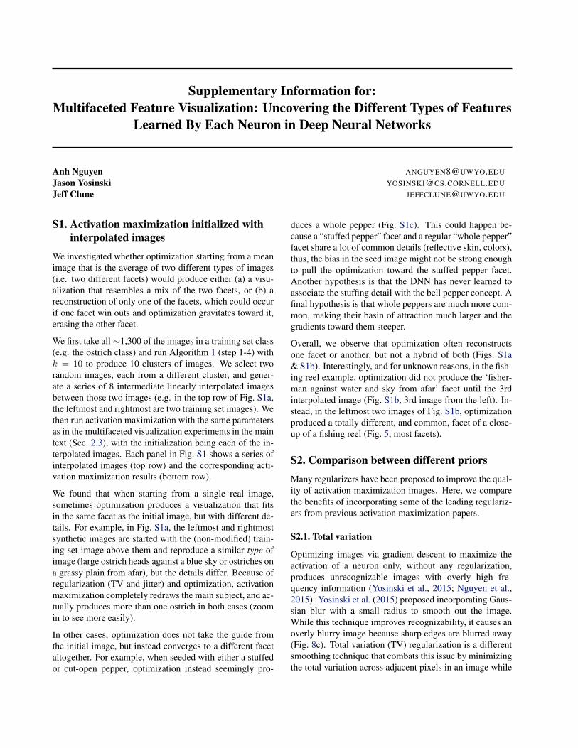
Anh Nguyen [email protected] Yosinski [email protected] Clune [email protected]

S1. Activation maximization initialized withinterpolated images

We investigated whether optimization starting from a meanimage that is the average of two different types of images(i.e. two different facets) would produce either (a) a visu-alization that resembles a mix of the two facets, or (b) areconstruction of only one of the facets, which could occurif one facet win outs and optimization gravitates toward it,erasing the other facet.

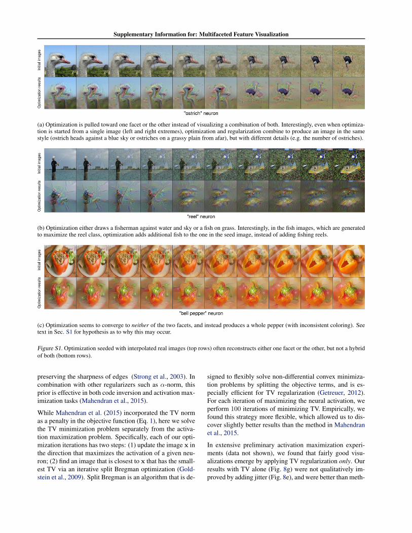
We first take all∼1,300 of the images in a training set class(e.g. the ostrich class) and run Algorithm 1 (step 1-4) withk = 10 to produce 10 clusters of images. We select tworandom images, each from a different cluster, and gener-ate a series of 8 intermediate linearly interpolated imagesbetween those two images (e.g. in the top row of Fig. S1a,the leftmost and rightmost are two training set images). Wethen run activation maximization with the same parametersas in the multifaceted visualization experiments in the maintext (Sec. 2.3), with the initialization being each of the in-terpolated images. Each panel in Fig. S1 shows a series ofinterpolated images (top row) and the corresponding acti-vation maximization results (bottom row).

We found that when starting from a single real image,sometimes optimization produces a visualization that fitsin the same facet as the initial image, but with different de-tails. For example, in Fig. S1a, the leftmost and rightmostsynthetic images are started with the (non-modified) train-ing set image above them and reproduce a similar type ofimage (large ostrich heads against a blue sky or ostriches ona grassy plain from afar), but the details differ. Because ofregularization (TV and jitter) and optimization, activationmaximization completely redraws the main subject, and ac-tually produces more than one ostrich in both cases (zoomin to see more easily).

In other cases, optimization does not take the guide fromthe initial image, but instead converges to a different facetaltogether. For example, when seeded with either a stuffedor cut-open pepper, optimization instead seemingly pro-

duces a whole pepper (Fig. S1c). This could happen be-cause a “stuffed pepper” facet and a regular “whole pepper”facet share a lot of common details (reflective skin, colors),thus, the bias in the seed image might not be strong enoughto pull the optimization toward the stuffed pepper facet.Another hypothesis is that the DNN has never learned toassociate the stuffing detail with the bell pepper concept. Afinal hypothesis is that whole peppers are much more com-mon, making their basin of attraction much larger and thegradients toward them steeper.

Overall, we observe that optimization often reconstructsone facet or another, but not a hybrid of both (Figs. S1a& S1b). Interestingly, and for unknown reasons, in the fish-ing reel example, optimization did not produce the ‘fisher-man against water and sky from afar’ facet until the 3rdinterpolated image (Fig. S1b, 3rd image from the left). In-stead, in the leftmost two images of Fig. S1b, optimizationproduced a totally different, and common, facet of a close-up of a fishing reel (Fig. 5, most facets).

S2. Comparison between different priorsMany regularizers have been proposed to improve the qual-ity of activation maximization images. Here, we comparethe benefits of incorporating some of the leading regulariz-ers from previous activation maximization papers.

S2.1. Total variation

Optimizing images via gradient descent to maximize theactivation of a neuron only, without any regularization,produces unrecognizable images with overly high fre-quency information (Yosinski et al., 2015; Nguyen et al.,2015). Yosinski et al. (2015) proposed incorporating Gaus-sian blur with a small radius to smooth out the image.While this technique improves recognizability, it causes anoverly blurry image because sharp edges are blurred away(Fig. 8c). Total variation (TV) regularization is a differentsmoothing technique that combats this issue by minimizingthe total variation across adjacent pixels in an image while

Supplementary Information for: Multifaceted Feature Visualization

(a) Optimization is pulled toward one facet or the other instead of visualizing a combination of both. Interestingly, even when optimiza-tion is started from a single image (left and right extremes), optimization and regularization combine to produce an image in the samestyle (ostrich heads against a blue sky or ostriches on a grassy plain from afar), but with different details (e.g. the number of ostriches).

(b) Optimization either draws a fisherman against water and sky or a fish on grass. Interestingly, in the fish images, which are generatedto maximize the reel class, optimization adds additional fish to the one in the seed image, instead of adding fishing reels.

(c) Optimization seems to converge to neither of the two facets, and instead produces a whole pepper (with inconsistent coloring). Seetext in Sec. S1 for hypothesis as to why this may occur.

Figure S1. Optimization seeded with interpolated real images (top rows) often reconstructs either one facet or the other, but not a hybridof both (bottom rows).

preserving the sharpness of edges (Strong et al., 2003). Incombination with other regularizers such as α-norm, thisprior is effective in both code inversion and activation max-imization tasks (Mahendran et al., 2015).

While Mahendran et al. (2015) incorporated the TV normas a penalty in the objective function (Eq. 1), here we solvethe TV minimization problem separately from the activa-tion maximization problem. Specifically, each of our opti-mization iterations has two steps: (1) update the image x inthe direction that maximizes the activation of a given neu-ron; (2) find an image that is closest to x that has the small-est TV via an iterative split Bregman optimization (Gold-stein et al., 2009). Split Bregman is an algorithm that is de-

signed to flexibly solve non-differential convex minimiza-tion problems by splitting the objective terms, and is es-pecially efficient for TV regularization (Getreuer, 2012).For each iteration of maximizing the neural activation, weperform 100 iterations of minimizing TV. Empirically, wefound this strategy more flexible, which allowed us to dis-cover slightly better results than the method in Mahendranet al., 2015.

In extensive preliminary activation maximization experi-ments (data not shown), we found that fairly good visu-alizations emerge by applying TV regularization only. Ourresults with TV alone (Fig. 8g) were not qualitatively im-proved by adding jitter (Fig. 8e), and were better than meth-


ods that predate Mahendran et al., 2015 (Fig. 8b-d).

S2.2. Jitter

An optimization regularization technique called “jitter”was first introduced by Mordvintsev et al., 2015 and laterused in Mahendran et al., 2015. The method involves: (1)creating a canvas (e.g. of size 272 × 272) that is largerthan the DNN input size (227 × 227) and (2) iterativelyoptimizing random 227 × 227 regions on the canvas. Op-timization with jitter often results in high-resolution, crispimages; however, it does not ameliorate the problems ofunnatural coloration and the repetition of image fragmentsthat do not form a coherent, sensible whole.

Because we believe it represents the best previous activa-tion maximization technique, we reproduce the algorithmof Mahendran et al. (2015), which applies both jitter andTV regularizers (Figs. S4a & 8e). Mahendran et al. (2015)report that TV is the most important prior in their frame-work. We found that Gaussian blur works just as well ifcombined with jitter while gradually reducing the blurringeffect (i.e. radius) during optimization (Fig. 8h). This com-bination works because: (1) as shown in Yosinski et al.(2015), the smoothing effect by Gaussian blur enables op-timization to find better local optima that have more globalstructure; (2) reducing the blur radius over time minimizesthe blurring artifact of this prior in the final result; and (3)jitter further enhances the sharpness of images.

S2.3. Center-biased regularization

Previous activation maximization methods produce imageswith many unnatural repeated image fragments (Fig. 8b-h).Though to a lesser degree, multifaceted feature visualiza-tion also produces such repetitions (Fig. 8k). Such rep-etitions are not found in the vast majority of training setimages. For example, a canonical training set image in the“beacon” class often shows a single lighthouse (Fig. 8a);however, Deep Visualization techniques show many morebeacons or patches of beacons (Fig. 8b-h, k). To amelioratethis issue, in this section we introduce a technique calledcenter-biased regularization.

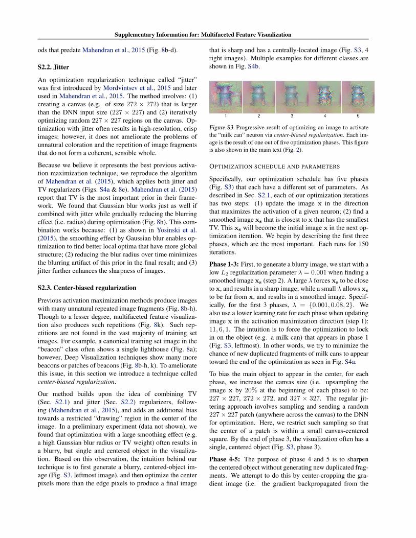
Our method builds upon the idea of combining TV(Sec. S2.1) and jitter (Sec. S2.2) regularizers, follow-ing (Mahendran et al., 2015), and adds an additional biastowards a restricted “drawing” region in the center of theimage. In a preliminary experiment (data not shown), wefound that optimization with a large smoothing effect (e.g.a high Gaussian blur radius or TV weight) often results ina blurry, but single and centered object in the visualiza-tion. Based on this observation, the intuition behind ourtechnique is to first generate a blurry, centered-object im-age (Fig. S3, leftmost image), and then optimize the centerpixels more than the edge pixels to produce a final image

that is sharp and has a centrally-located image (Fig. S3, 4right images). Multiple examples for different classes areshown in Fig. S4b.

Figure S3. Progressive result of optimizing an image to activatethe “milk can” neuron via center-biased regularization. Each im-age is the result of one out of five optimization phases. This figureis also shown in the main text (Fig. 2).

OPTIMIZATION SCHEDULE AND PARAMETERS

Specifically, our optimization schedule has five phases(Fig. S3) that each have a different set of parameters. Asdescribed in Sec. S2.1, each of our optimization iterationshas two steps: (1) update the image x in the directionthat maximizes the activation of a given neuron; (2) find asmoothed image xs that is closest to x that has the smallestTV. This xs will become the initial image x in the next op-timization iteration. We begin by describing the first threephases, which are the most important. Each runs for 150iterations.

Phase 1-3: First, to generate a blurry image, we start with alow L2 regularization parameter λ = 0.001 when finding asmoothed image xs (step 2). A large λ forces xs to be closeto x, and results in a sharp image; while a small λ allows xs

to be far from x, and results in a smoothed image. Specif-ically, for the first 3 phases, λ = {0.001, 0.08, 2}. Wealso use a lower learning rate for each phase when updatingimage x in the activation maximization direction (step 1):11, 6, 1. The intuition is to force the optimization to lockin on the object (e.g. a milk can) that appears in phase 1(Fig. S3, leftmost). In other words, we try to minimize thechance of new duplicated fragments of milk cans to appeartoward the end of the optimization as seen in Fig. S4a.

To bias the main object to appear in the center, for eachphase, we increase the canvas size (i.e. upsampling theimage x by 20% at the beginning of each phase) to be:227 × 227, 272 × 272, and 327 × 327. The regular jit-tering approach involves sampling and sending a random227× 227 patch (anywhere across the canvas) to the DNNfor optimization. Here, we restrict such sampling so thatthe center of a patch is within a small canvas-centeredsquare. By the end of phase 3, the visualization often has asingle, centered object (Fig. S3, phase 3).

Phase 4-5: The purpose of phase 4 and 5 is to sharpenthe centered object without generating new duplicated frag-ments. We attempt to do this by center-cropping the gra-dient image (i.e. the gradient backpropagated from the


DNN has the form of a 3 × 227 × 227 image) down to3 × 127 × 127. In addition, in phase 4, we restrict the op-timization to the center of the image only, and optimize for30 iterations. That sharpens the region in the image center(Fig. S3, phase 4). Finally, to balance out the sharpness be-tween the center and edge pixels, in phase 5, we optimizefor 10 iterations while allowing jittering to occur anywherein the image. Thus, the final visualization is often a sharperversion of the phase 3 result (Fig. S3, phase 5 vs phase 3).

The center-biased regularized images have far fewer du-plicated fragments (Fig. 8i). They thus more closely rep-resent the style of training set images, which feature onecentrally located object. However, this technique is notguaranteed to produce a single object only. Instead, it isa way of biasing optimization toward creating objects nearthe image center. Sec. S2.4 shows the experiment combin-ing center-biased regularization and multifaceted visualiza-tion (initializing from mean images) to further improve thevisualization quality.

S2.4. Initialization with mean images

An issue with previous activation maximization methods isthat the images tend to have an unrealistic color distribu-tion (Fig. 8b-c, e-h). A straightforward approach to ame-liorate this problem is to incorporate an α-norm regularizer,which encourages the intensity of pixels to stay within agiven range (Mahendran et al., 2015; Yosinski et al., 2015).While this method is effective in suppressing extreme colorvalues, it does not improve the realism of the overall colordistribution of images. Wei et al., 2015 proposed a more ad-vanced data-driven patch prior regularization to enforce thevisualizations to match the colors of a set of natural imagepatches. While this prior substantially improved the colorsfor code inversion, its results for activation maximizationstill have several issues (as seen in Fig. 8d): (1) having du-plicated fragments (e.g. duplicated patches of lighthousesin a “beacon” image), and (2) lacking details, producingunnatural images.

Here, our multifaceted visualization improves the color dis-tribution of images via a different approach: starting op-timization from a mean image (Fig. S4d) computed fromreal training examples (see Sec. 3.3). A possible explana-tion for why this works is that initializing from the meanimage puts the search in a low-dimensional manifold thatis much closer to that of real images, and thus it is eas-ier to find a realistic looking image around this area. Themean image thus provides a general outline for a type ofimage based on blurry colors and optimization can fill inthe details. For example, the center-biased regularizationtechnique was able to produce a single milk can, but did sowithout a relevant contextual setting (Fig. S4b). However,when this technique is initialized with a mean image (com-

puted from 15 images from the “milk can” class) that hasa blurry brown surface (Fig. S4d, milk can), optimizationturned that general layout into a complete, coherent picture:a milk can on a table (Fig. S4c). The colors of the visual-izations are also substantially improved when optimizationis initialized from mean images (Fig. S4b versus Fig. S4c).

We observed that multifaceted visualization images oftenexhibit centered objects (Fig. 1 & 3), and thus we found nosubstantial qualitative improvement when adding center-biased regularization to it (Fig. S4c). That could be becausethe mean image provides enough of a global layout for thestyle of the image, which in ImageNet is usually a single,centered object.

While simple, our technique results in images that havequalitatively more realistic colors than previous methods(Figs. 7 & 8k). This technique is also expected to workwith any dataset (e.g. grayscale images, or images of aspecial topic).

Note that multifaceted feature visualization does not re-quire access to the training set. If the training set is un-available, one can simply pass any natural images (or othermodes of input such as audio if not reconstructing images)to get a set of images (or other input types) that highly acti-vate a neuron. A similar idea was used in Wei et al. (2015),who built an external dataset of patches that have similarcharacteristics to the DNN training set.


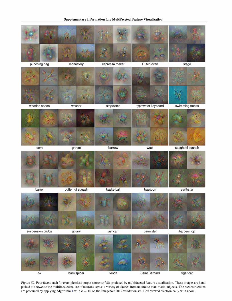
Figure S2. Four facets each for example class output neurons (fc8) produced by multifaceted feature visualization. These images are handpicked to showcase the multifaceted nature of neurons across a variety of classes from natural to man-made subjects. The reconstructionsare produced by applying Algorithm 1 with k = 10 on the ImageNet 2012 validation set. Best viewed electronically with zoom.


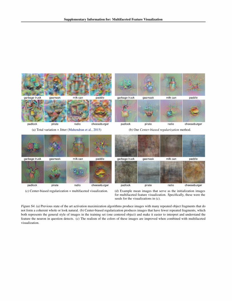
(a) Total variation + Jitter (Mahendran et al., 2015) (b) Our Center-biased regularization method.

(c) Center-biased regularization + multifaceted visualization. (d) Example mean images that serve as the initialization imagesfor multifaceted feature visualization. Specifically, these were theseeds for the visualizations in (c).

Figure S4. (a) Previous state of the art activation maximization algorithms produce images with many repeated object fragments that donot form a coherent whole or look natural. (b) Center-biased regularization produces images that have fewer repeated fragments, whichboth represents the general style of images in the training set (one centered object) and make it easier to interpret and understand thefeature the neuron in question detects. (c) The realism of the colors of these images are improved when combined with multifacetedvisualization.


S3. What are the hidden units in fullyconnected layers for?

We reported in the main text (Sec. 3.2) that neurons in hid-den, fully connected layers often seem to be an amalgamof very different, abstract concepts. For example, a recon-struction of one of the facets of a neuron in fc6 looks likea combination of a scuba diver and a turtle (Fig. 6, left-most fc6 neuron). Here, we document a series of visual-ization experiments that we performed to further shed lighton the inner-workings of hidden, fully connected neurons(in our model, the neurons on fc6 and fc7), such as thosevisualized in Fig. 6.

The reconstructions for neurons in hidden layers (Fig. 6)were produced by running Algorithm 1 with k = 10 clus-ters on the top 1000 validation set images that most highlyactivate each hidden neuron. To understand what featurea neuron fires in response to, we can look at the differ-ent types of images that highly activate it (i.e. its differ-ent facets). Fig. S5 shows, for each cluster of images thathighly activate a neuron, 4 random images from that clus-ter. Specifically, we show 4 random images from the setof 15 images that were averaged to compute the mean im-age that optimization is initialized with when visualizingthat facet. This visualization method is similar to the ap-proach of visualizing the top 9 images that activate a neu-ron from Zeiler et al. (2014), except it is per facet.

We observe that many individual fc6 and fc7 neurons firefor very different types of images. For example, the fc6unit that resembles a combination of a scuba diver and aturtle (Fig. S5c, left neuron) does indeed fire for turtles andscuba divers, but also for sharks, bells, human faces andeven trucks. Even when multifaceted feature visualizationis seeded with a mean image of very different concepts,such as human faces or automobiles, optimization for thisneuron consistently converges to very similar images thatresemble a turtle with goggles (Fig. S5c, left).

In contrast, and as we would expect given that they aretrained to fire in response to one type of image, neuronson the fc8 layer more clearly represent the same seman-tic concept. For these neurons, unlike with fc6 and fc7neurons, multifaceted feature visualization produces veryunique facet reconstructions for fc8 neurons that representdifferent facets of the same semantic concept (Fig. S2). Forexample, the “restaurant” class neuron responds to inte-rior views of an entire restaurant in daylight and at night(Fig. S5a, top two rows), and to close-up views of plates offood (Fig. S5a, bottom two rows). In these cases, and alsofor convolutional layers, multifaceted feature reconstruc-tions closely reflect the content of the real images in eachfacet. In other words, optimization stays near the initialimage it is seeded with.

In some cases, however, even fc8 neurons respond to an oddassortment of different types of images. For example, the“ostrich” class neuron fires highly for many non-ostrich im-ages like leopards and lizards (Fig. S5a, right panel). Evenwhen viewing the top 9 images that activate a class neuron(ignoring facets), there is usually at least one image fromanother class, even though there are at least 50 images fromthat class in the 50, 000-image validation set. Because ourMFV algorithm performs clusters on far more than 9 im-ages, some of these clusters will represent an entire groupof images that are not of that class (e.g. a “lizard” facet forthe ostrich neuron). Often, when MFV initializes optimiza-tion with the mean image of those non-class images, opti-mization “walks away” from that starting point to producean image of the class: many examples of this are shown inFig. S5, such as optimization producing images of ostricheseven when seeded with a mean image from a facet of non-ostrich birds or even a facet composed mostly of wild dogs,cows, and giraffes.

While informative, these cluster images could also be mis-leading because it is not clear whether a given neuron firesfor very different types of images (Fig. S5c, photocopiers,trucks, dogs, etc.) or whether that neuron instead fires be-cause there is a common feature present in those differentimages. We attempted to visualize the pixels in each im-age that are most responsible for that neuron firing via thedeconvolution technique (Zeiler et al., 2014) and via Layer-wise Relevance Propagation (LRP) (Bach et al., 2015a)(Fig. S6). The Deconv results are produced via the Deep-Vis toolbox (Yosinski et al., 2015), and the LRP results areproduced by the LRP toolbox (Bach et al., 2015b).

Unfortunately, deconvolution visualizations often contain alot of noise that makes it hard to identify the most impor-tant regions in an image (Fig. S6, bottom row). This ob-servation agrees with a recent evaluation of deconv (Sameket al., 2015). For this reason, we also visualize the imageswith LRP algorithm. The LRP heatmaps are also difficultto interpret. For example, for the fc6 “scuba diver and tur-tle” neuron, they show that the outlines of very differentshapes cause this neuron to fire, including shapes of under-water things like scuba divers, sharks and turtles (Fig. S6a,top row in LRP panel), but also a metal bell, human heads,and automobile wheels (Fig. S6a, LRP panel). It is possiblethat the neuron cares about the semantics of those disparateobject types, or simply that it fires in response to a circu-lar outline pattern that vaguely resembles goggles, which ispresent in most of these images (albeit at different scales).Another mutually exclusive hypothesis for why the recon-structions are not easily interpretable is that these neuronsare part of highly distributed representations. Ultimately, itis unclear exactly what feature this neuron detects.

Our conclusion remains the same for many other fc6 and


fc7 units (see also Fig. S6b): while it is unclear exactlywhat they represent, these neurons do seem to represent anamalgam of different types of images, and optimization of-ten produces the same hybrid visualization no matter whereit is started from, such as the yellow dog+bathtub on fc6(Fig. S5c). Other times there is a dominant visualizationthat also appears no matter where optimization starts, butthat is more semantically homogeneous (instead of being ahybrid of very different concepts), such as an arch or quail-like bird (Fig. S5b).

Overall, the evidence in this section reveals how little weknow about the precise function of hidden neurons in fullyconnected layers, and future research is required to makeprogress on this interesting question.


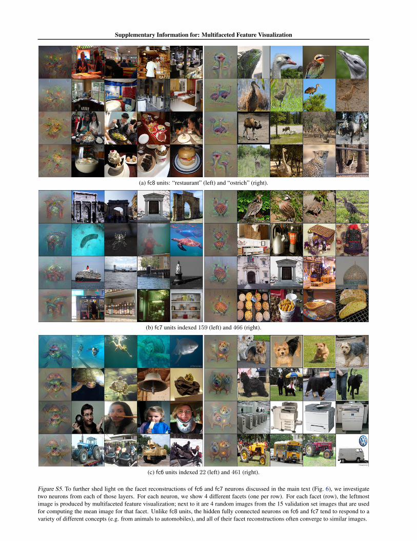
(a) fc8 units: “restaurant” (left) and “ostrich” (right).

(b) fc7 units indexed 159 (left) and 466 (right).

(c) fc6 units indexed 22 (left) and 461 (right).

Figure S5. To further shed light on the facet reconstructions of fc6 and fc7 neurons discussed in the main text (Fig. 6), we investigatetwo neurons from each of those layers. For each neuron, we show 4 different facets (one per row). For each facet (row), the leftmostimage is produced by multifaceted feature visualization; next to it are 4 random images from the 15 validation set images that are usedfor computing the mean image for that facet. Unlike fc8 units, the hidden fully connected neurons on fc6 and fc7 tend to respond to avariety of different concepts (e.g. from animals to automobiles), and all of their facet reconstructions often converge to similar images.


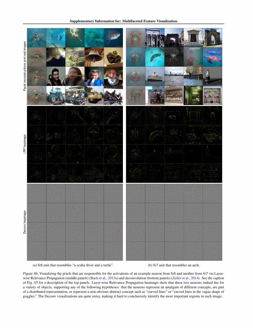
(a) fc6 unit that resembles “a scuba diver and a turtle”. (b) fc7 unit that resembles an arch.

Figure S6. Visualizing the pixels that are responsible for the activations of an example neuron from fc6 and another from fc7 via Layer-wise Relevance Propagation (middle panels) (Bach et al., 2015a) and deconvolution (bottom panels) (Zeiler et al., 2014). See the captionof Fig. S5 for a description of the top panels. Layer-wise Relevance Propagation heatmaps show that these two neurons indeed fire fora variety of objects, supporting any of the following hypotheses: that the neurons represent an amalgam of different concepts, are partof a distributed representation, or represent a non-obvious abstract concept such as “curved lines” or “curved lines in the vague shape ofgoggles.” The Deconv visualizations are quite noisy, making it hard to conclusively identify the most important regions in each image.

multifaceted feature visualization: uncovering the ...multifaceted feature visualization: uncovering...

Documents