Multiclass Logistic Regression

Sargur N. Srihari University at Buffalo, State University of New York

USA

Topics in Linear Classification using Probabilistic Discriminative Models

•  Generative vs Discriminative 1.  Fixed basis functions in linear classification 2.  Logistic Regression (two-class) 3.  Iterative Reweighted Least Squares (IRLS) 4.  Multiclass Logistic Regression 5.  Probit Regression 6.  Canonical Link Functions

2

Srihari Machine Learning

Topics in Multiclass Logistic Regression

•  Multiclass Classification Problem •  Softmax Regression •  Softmax Regression Implementation •  Softmax and Training •  One-hot vector representation •  Objective function and gradient •  Summary of concepts in Logistic Regression •  Example of 3-class Logistic Regression

Machine Learning Srihari

3

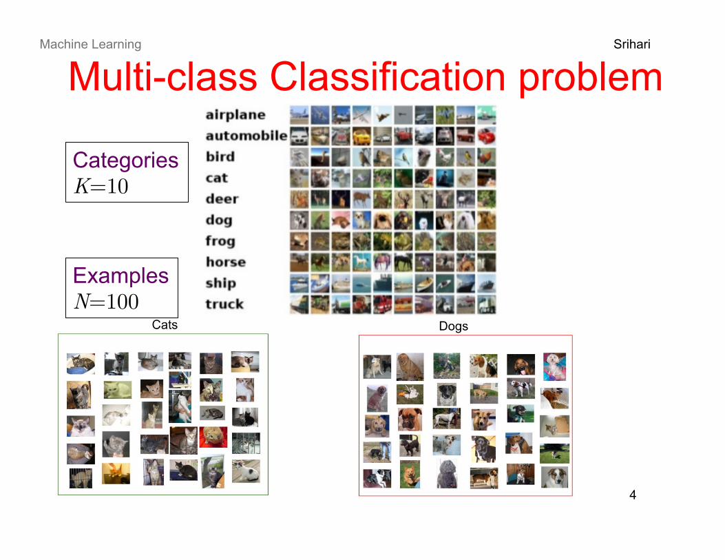
Multi-class Classification problem Machine Learning Srihari

4

Categories K=10

Examples N=100

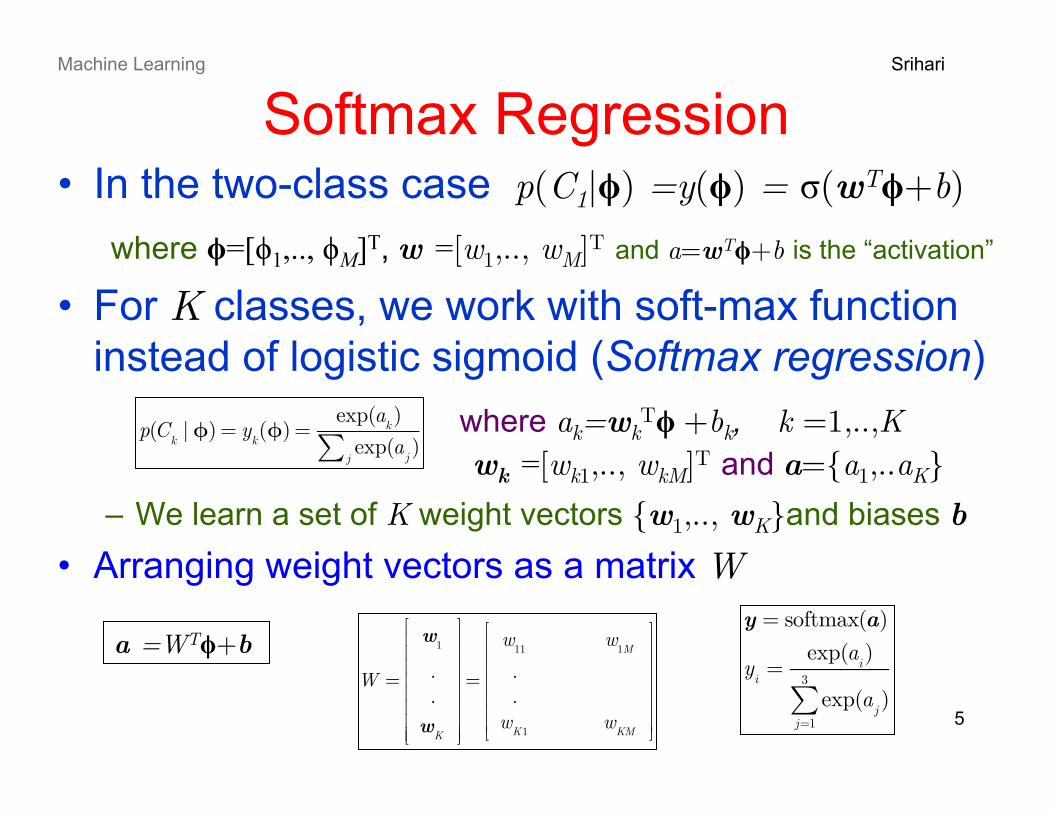
Softmax Regression •  In the two-class case p(C1|ϕ) =y(ϕ) = σ(wTϕ+b)

where ϕ=[ϕ1,.., ϕM]T, w =[w1,.., wM]T and a=wTϕ+b is the “activation”

•  For K classes, we work with soft-max function instead of logistic sigmoid (Softmax regression)

where ak=wkTϕ +bk, k =1,..,K

–  We learn a set of K weight vectors {w1,.., wK}and biases b

•  Arranging weight vectors as a matrix W

5

Srihari

p(C

k| φ) = y

k(φ) =

exp(ak)

exp(aj)

j∑

Machine Learning

a =WTϕ+b

y = softmax(a)

yi

=exp(a

i)

exp(aj)

j=1

3

∑

W =

w1

.

.

wK

⎡

⎣

⎢⎢⎢⎢⎢⎢⎢⎢

⎤

⎦

⎥⎥⎥⎥⎥⎥⎥⎥

=

w11

w1M

.

.w

K1w

KM

⎡

⎣

⎢⎢⎢⎢⎢⎢⎢

⎤

⎦

⎥⎥⎥⎥⎥⎥⎥

wk =[wk1,.., wkM]T and a={a1,..aK}

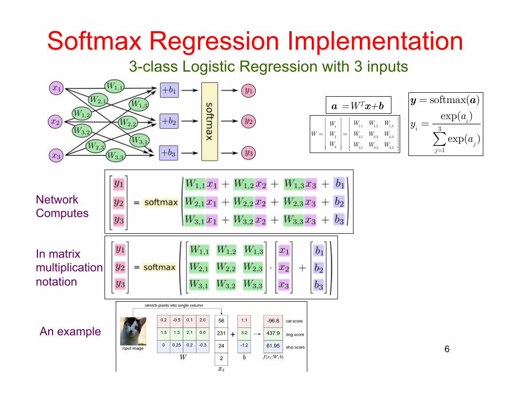
Softmax Regression Implementation

6

a =WTx+b

y = softmax(a)

yi

=exp(a

i)

exp(aj)

j=1

3

∑

Network Computes

In matrix multiplication notation

3-class Logistic Regression with 3 inputs

An example

W =

W1

W2

W3

⎡

⎣

⎢⎢⎢⎢⎢⎢

⎤

⎦

⎥⎥⎥⎥⎥⎥

=

W1.1

W1,2

W1,3

W2,1

W2.2

W2,3

W3,1

W3,2

W3,3

⎡

⎣

⎢⎢⎢⎢⎢⎢

⎤

⎦

⎥⎥⎥⎥⎥⎥

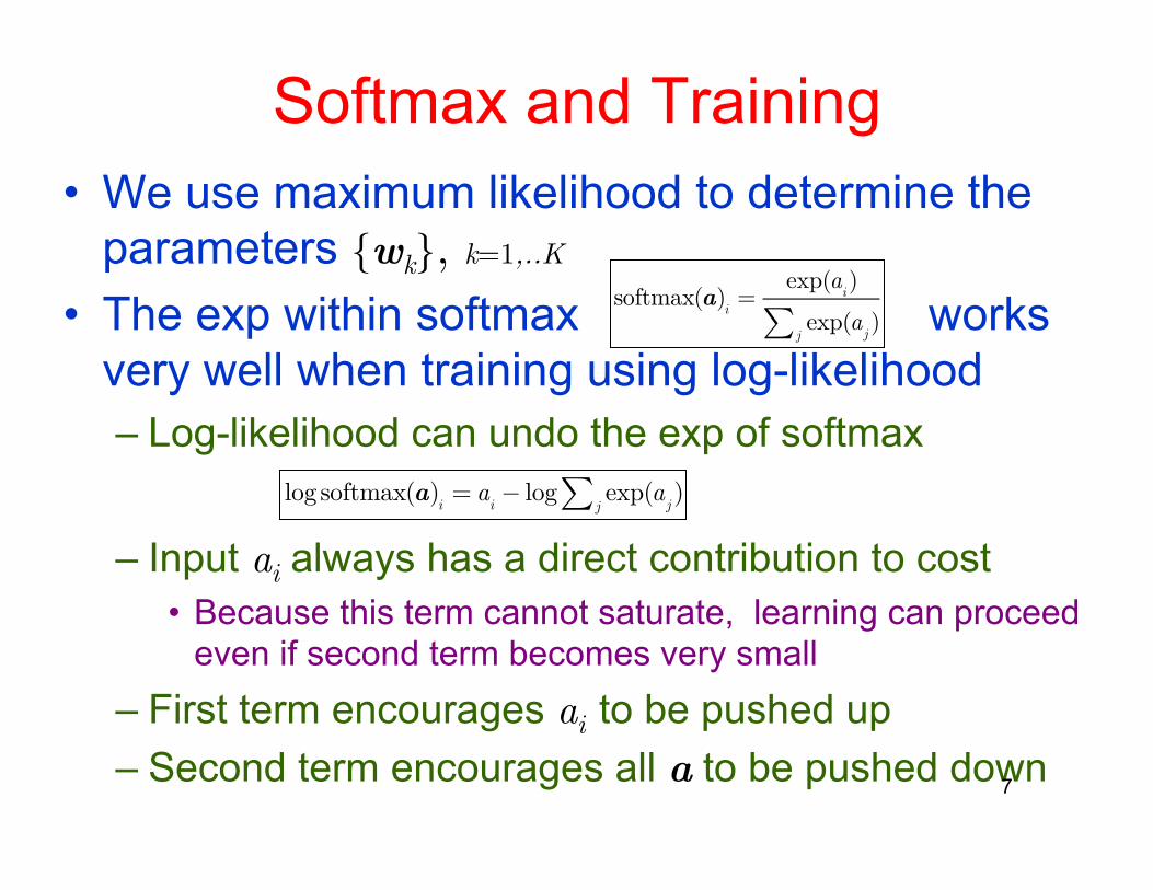
Softmax and Training •  We use maximum likelihood to determine the

parameters {wk}, k=1,..K

•  The exp within softmax works very well when training using log-likelihood – Log-likelihood can undo the exp of softmax

–  Input ai always has a direct contribution to cost

•  Because this term cannot saturate, learning can proceed even if second term becomes very small

– First term encourages ai to be pushed up – Second term encourages all a to be pushed down 7

log softmax(a)

i= a

i− log exp(a

jj∑ )

softmax(a)i

=exp(a

i)

exp(aj)

j∑

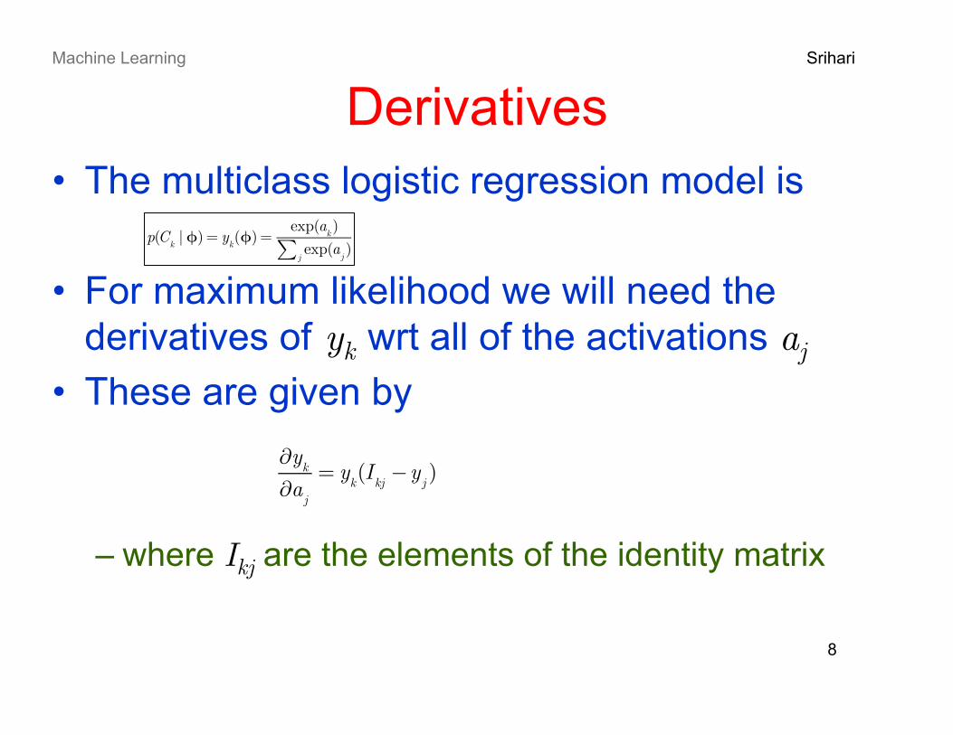
Derivatives •  The multiclass logistic regression model is

•  For maximum likelihood we will need the derivatives of yk wrt all of the activations aj

•  These are given by

– where Ikj are the elements of the identity matrix

Machine Learning Srihari

8

∂yk

∂aj

= yk(I

kj−y

j)

p(C

k| φ) = y

k(φ) =

exp(ak)

exp(aj)

j∑

9

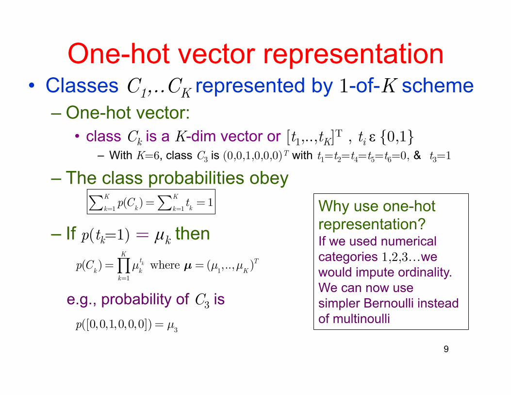
One-hot vector representation •  Classes C1,..CK represented by 1-of-K scheme

– One-hot vector: •  class Ck is a K-dim vector or [t1,..,tK]T , ti ε {0,1}

–  With K=6, class C3 is (0,0,1,0,0,0)T with t1=t2=t4=t5=t6=0, & t3=1

– The class probabilities obey

–  If p(tk=1) = µk then

p(C

k) = µ

k

tk

k=1

K

∏ where µ = (µ1,..,µ

K)T

e.g., probability of C3 is

p(C

kk=1

K∑ ) = tkk=1

K∑ = 1

p([0,0,1,0,0,0]) = µ3

Why use one-hot representation? If we used numerical categories 1,2,3…we would impute ordinality. We can now use simpler Bernoulli instead of multinoulli

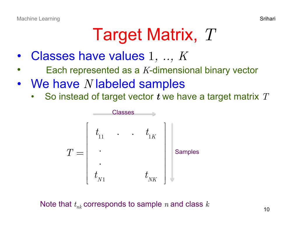
Target Matrix, T Machine Learning Srihari

10

T =

t11

. . t1K

.

.tN1

tNK

⎡

⎣

⎢⎢⎢⎢⎢⎢⎢

⎤

⎦

⎥⎥⎥⎥⎥⎥⎥

•  Classes have values 1, .., K •  Each represented as a K-dimensional binary vector •  We have N labeled samples

•  So instead of target vector t we have a target matrix T

Classes

Samples

Note that tnk corresponds to sample n and class k

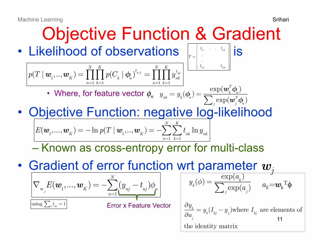
Objective Function & Gradient •  Likelihood of observations is

•  Where, for feature vector φn

Srihari

11

p(T |w

1,..,w

K) = p(C

k|φ

n)tn ,k

k=1

K

∏n=1

N

∏ = ynk

tnk

k=1

K

∏n=1

N

∏

Machine Learning

ynk

= yk(φ

n) =

exp(wkTφ

n)

exp(wjTφ

n)

j∑

T =

t11

. . t1K

.

.tN1

tNK

⎡

⎣

⎢⎢⎢⎢⎢⎢⎢

⎤

⎦

⎥⎥⎥⎥⎥⎥⎥

•  Objective Function: negative log-likelihood

– Known as cross-entropy error for multi-class •  Gradient of error function wrt parameter wj

E(w

1,...,w

K) =− ln p(T |w

1,..,w

K) =− t

nklny

nkk=1

K

∑n=1

N

∑

∇

w jE(w

1,...,w

K) =− (y

nj− t

nj)φ

nn=1

N

∑Error x Feature Vector

using tnkk∑ = 1

∂yk

∂aj

= yk(I

kj−y

j)where I

kj are elements of

the identity matrix

y

k(φ) =

exp(ak)

exp(aj)

j∑ ak=wkTϕ

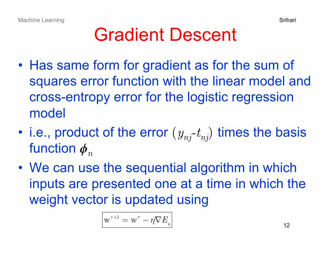
Gradient Descent •  Has same form for gradient as for the sum of

squares error function with the linear model and cross-entropy error for the logistic regression model

•  i.e., product of the error (ynj-tnj) times the basis function ϕn

•  We can use the sequential algorithm in which inputs are presented one at a time in which the weight vector is updated using

Machine Learning Srihari

12 wτ+1 = wτ − η∇E

n

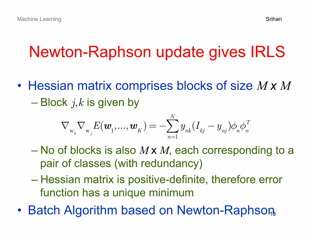
Newton-Raphson update gives IRLS

•  Hessian matrix comprises blocks of size M x M – Block j,k is given by

– No of blocks is also M x M, each corresponding to a pair of classes (with redundancy)

– Hessian matrix is positive-definite, therefore error function has a unique minimum

•  Batch Algorithm based on Newton-Raphson

Srihari

13

∇

wk∇

w jE(w

1,...,w

K) =− y

nk(I

kj−y

nj)φ

nn=1

N

∑ φnT

Machine Learning

Summary of Logistic Regression concepts

•  Definition of gradient and Hessian •  Gradient and Hessian in Linear Regression •  Gradient and Hessian in 2-class Logistic

Regression

Machine Learning Srihari

14

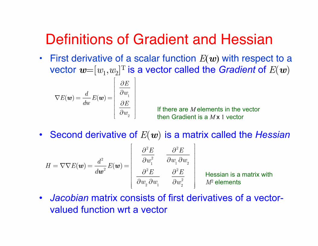
Definitions of Gradient and Hessian•  First derivative of a scalar function E(w) with respect to a

vector w=[w1,w2]T is a vector called the Gradient of E(w)

•  Second derivative of E(w) is a matrix called the Hessian

•  Jacobian matrix consists of first derivatives of a vector-valued function wrt a vector

∇E(w) =ddw

E(w) =

∂E∂w

1

∂E∂w

2

⎡

⎣

⎢⎢⎢⎢⎢⎢⎢

⎤

⎦

⎥⎥⎥⎥⎥⎥⎥

H =∇∇E(w) =d

2

dw2E(w) =

∂2E

∂w12

∂2E

∂w1∂w

2

∂2E

∂w2∂w

1

∂2E

∂w22

⎡

⎣

⎢⎢⎢⎢⎢⎢⎢⎢

⎤

⎦

⎥⎥⎥⎥⎥⎥⎥⎥

If there are M elements in the vector then Gradient is a M x 1 vector

Hessian is a matrix with M2 elements

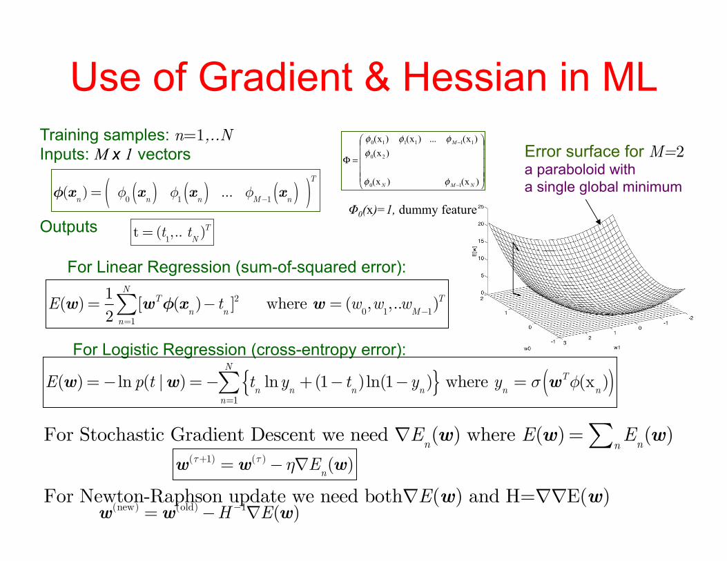
Use of Gradient & Hessian in ML Error surface for M=2 a paraboloid with a single global minimum

For Stochastic Gradient Descent we need ∇En(w) where E(w) = E

n(w)

n∑

For Newton-Raphson update we need both∇E(w) and H=∇∇E(w)

E(w) =

12

[wTφ(xn)− t

n]2

n=1

N

∑ where w = (w0,w

1,..w

M−1)T

φ(x

n) = φ

0x

n( ) φ1x

n( ) ... φM−1

xn( )( )

T

For Linear Regression (sum-of-squared error):

Training samples: n=1,..N Inputs: M x 1 vectors Outputs

t = (t1,.. t

N)T

w(new) = w(old)−H

−1∇E(w)

w(τ+1) = w(τ)− η∇E

n(w)

For Logistic Regression (cross-entropy error):

E(w) =− ln p(t |w) =− t

nlny

n+ (1− t

n)ln(1−y

n){ }

n=1

N

∑ where yn

= σ wTφ(xn)( )

⎟⎟⎟⎟⎟

⎠

⎞

⎜⎜⎜⎜⎜

⎝

⎛

=Φ

−

−

)x()x(

)x()x(...)x()x(

10

20

111110

NMN

M

φφ

φφφφ

Φ0(x)=1, dummy feature

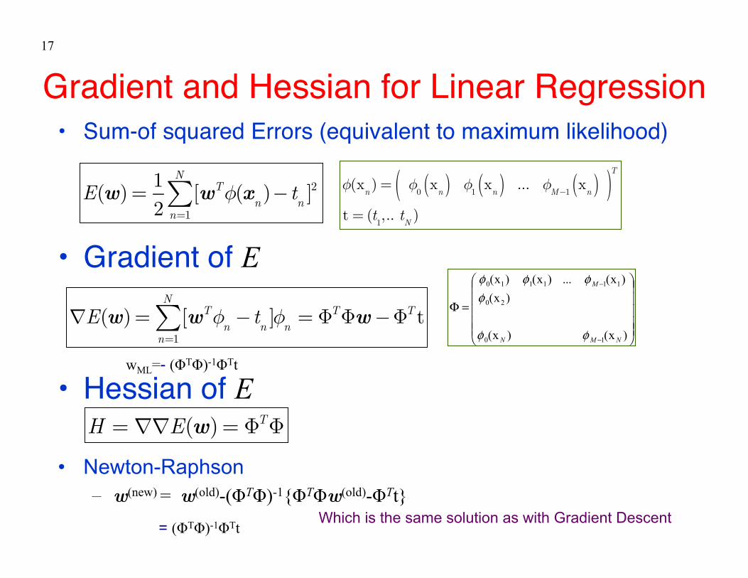
Gradient and Hessian for Linear Regression•  Sum-of squared Errors (equivalent to maximum likelihood)

•  Gradient of E

•  Hessian of E •  Newton-Raphson

–  w(new) = w(old)-(ΦTΦ)-1{ΦTΦw(old)-ΦTt}

= (ΦTΦ)-1ΦTt

17

E(w) =

12

[wTφ(xn)− t

n]2

n=1

N

∑

∇E(w) = [wTφ

n− t

n]φ

nn=1

N

∑ = ΦTΦw−ΦTt⎟⎟⎟⎟⎟

⎠

⎞

⎜⎜⎜⎜⎜

⎝

⎛

=Φ

−

−

)x()x(

)x()x(...)x()x(

10

20

111110

NMN

M

φφ

φφφφ

φ(xn)= φ

0xn( ) φ1

xn( ) ... φ

M−1xn( )( )

T

t = (t1,.. t

N)

H =∇∇E(w) = ΦTΦ

Which is the same solution as with Gradient Descent

wML=- (ΦTΦ)-1ΦTt

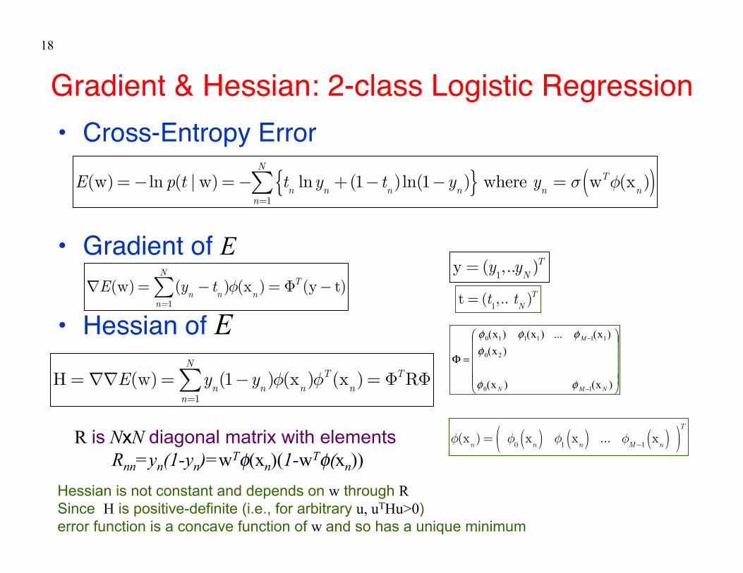
Gradient & Hessian: 2-class Logistic Regression•  Cross-Entropy Error

•  Gradient of E

•  Hessian of E

18

⎟⎟⎟⎟⎟

⎠

⎞

⎜⎜⎜⎜⎜

⎝

⎛

=Φ

−

−

)x()x(

)x()x(...)x()x(

10

20

111110

NMN

M

φφ

φφφφ

E(w) =− ln p(t | w) =− t

nlny

n+ (1− t

n)ln(1−y

n){ }

n=1

N

∑ where yn

= σ wTφ(xn)( )

∇E(w) = (y

n− t

n)φ(x

n) = ΦT(y− t)

n=1

N

∑

H =∇∇E(w) = y

n(1−y

n)φ(x

n)φT

(xn) = ΦT

RΦn=1

N

∑

R is NxN diagonal matrix with elements Rnn=yn(1-yn)=wTφ(xn)(1-wTφ(xn))

y = (y1,..y

N)T

t = (t1,.. t

N)T

φ(x

n) = φ

0x

n( ) φ1x

n( ) ... φM−1

xn( )( )

T

Hessian is not constant and depends on w through R Since H is positive-definite (i.e., for arbitrary u, uTHu>0) error function is a concave function of w and so has a unique minimum

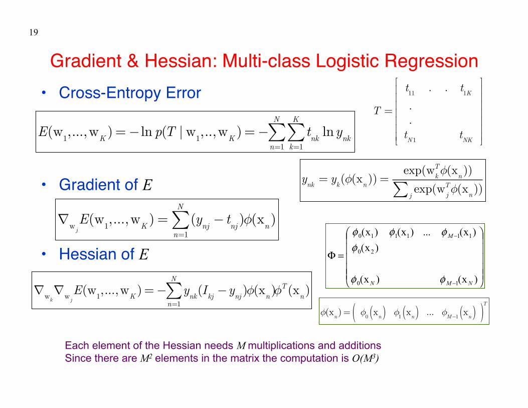
Gradient & Hessian: Multi-class Logistic Regression•  Cross-Entropy Error

•  Gradient of E

•  Hessian of E

19

⎟⎟⎟⎟⎟

⎠

⎞

⎜⎜⎜⎜⎜

⎝

⎛

=Φ

−

−

)x()x(

)x()x(...)x()x(

10

20

111110

NMN

M

φφ

φφφφ

E(w

1,...,w

K) =− ln p(T | w

1,..,w

K) =− t

nklny

nkk=1

K

∑n=1

N

∑

∇w jE(w

1,...,w

K)= (y

nj− t

nj)φ(x

nn=1

N

∑ )

T =

t11

. . t1K

.

.tN1

tNK

⎡

⎣

⎢⎢⎢⎢⎢⎢⎢

⎤

⎦

⎥⎥⎥⎥⎥⎥⎥

ynk= y

k(φ(x

n))=

exp(wkTφ(x

n))

exp(wjTφ(x

n))

j∑

∇

wk∇

w jE(w

1,...,w

K) =− y

nk(I

kj−y

nj)φ(x

n)

n=1

N

∑ φT(xn)

φ(x

n) = φ

0x

n( ) φ1x

n( ) ... φM−1

xn( )( )

T

Each element of the Hessian needs M multiplications and additions Since there are M2 elements in the matrix the computation is O(M3)

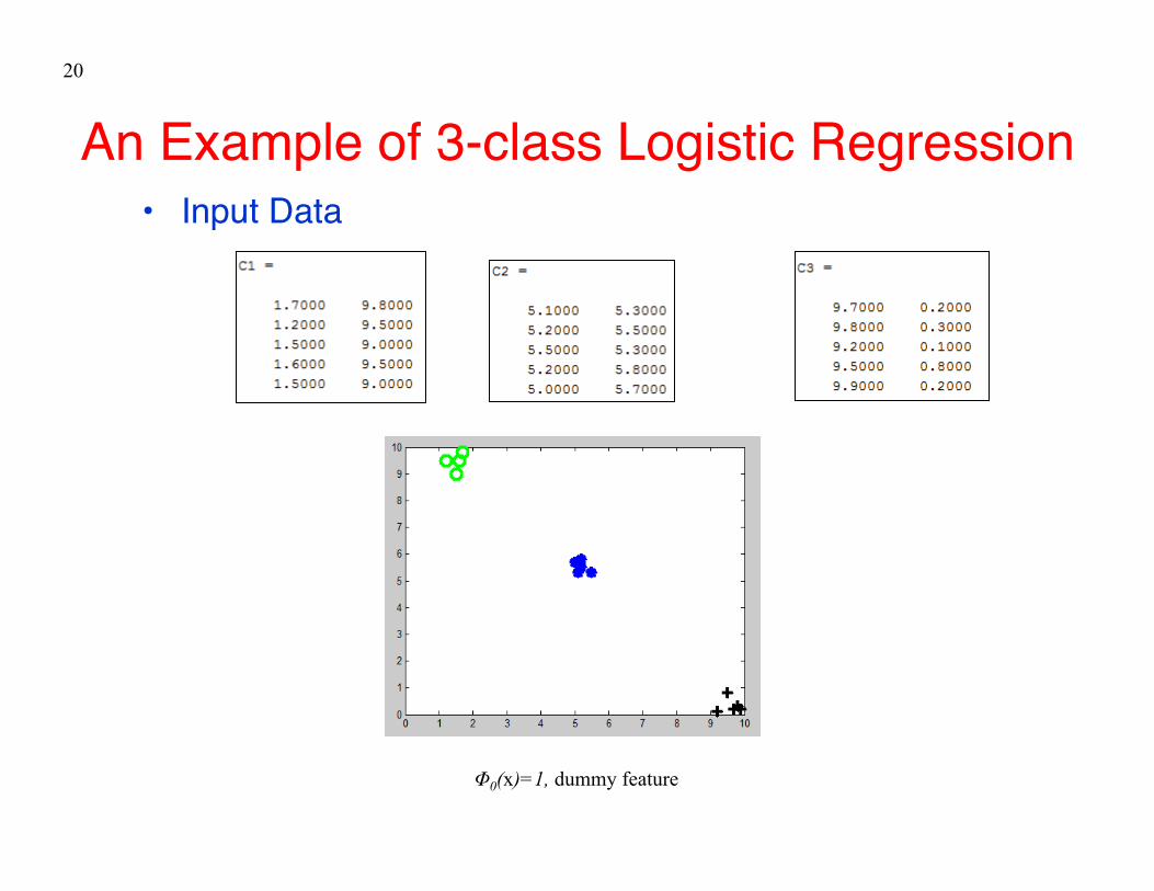
An Example of 3-class Logistic Regression•  Input Data

20

Φ0(x)=1, dummy feature

Three-class Logistic Regression•  Three weight vectors (Initial)

•  Gradient

•  Hessian (9x9 with some 3 x 3 blocks repeated)

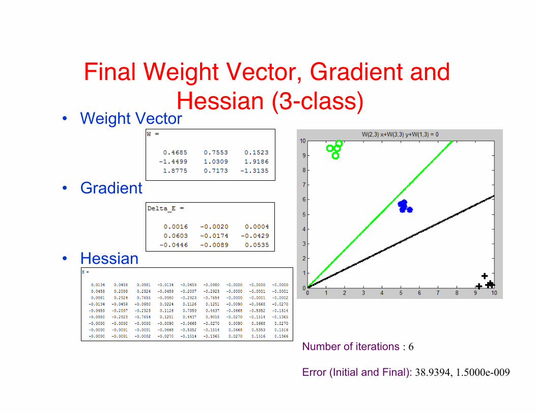
Final Weight Vector, Gradient and Hessian (3-class)

•  Weight Vector

•  Gradient

•  Hessian

Number of iterations : 6 Error (Initial and Final): 38.9394, 1.5000e-009