AI and Neural Networks

(Assignment –I)

Submitted in partial fulfilment of the requirements for the degree of

Master of Technology in Information Technology

by

Vijayananda D Mohire

(Enrolment No.921DMTE0113)

Information Technology Department

Karnataka State Open University

Manasagangotri, Mysore – 570006

Karnataka, India

(2010)

MT22-I

2

AI and Neural Networks

MT22-I

3

CERTIFICATE

This is to certify that the Assignment-I entitled AI and Neural Networks, subject

code: MT22 submitted by Vijayananda D Mohire having Roll Number

921DMTE0113 for the partial fulfilment of the requirements of Master of

Technology in Information Technology degree of Karnataka State Open University,

Mysore, embodies the bonafide work done by him under my supervision.

Place: ________________ Signature of the Internal Supervisor

Name

Date: ________________ Designation

MT22-I

4

For Evaluation

Question

Number

Maximum Marks Marks awarded Comments, if any

1 1

2 1

3 1

4 1

5 1

6 1

7 1

8 1

9 1

10 1

TOTAL 10

Evaluator’s Name and Signature Date

MT22-I

5

Preface

This document has been prepared specially for the assignments of M.Tech – IT II

Semester. This is mainly intended for evaluation of assignment of the academic

M.Tech - IT, II semester. I have made a sincere attempt to gather and study the

best answers to the assignment questions and have attempted the responses to

the questions. I am confident that the evaluator’s will find this submission

informative and evaluate based on the provide content.

For clarity and ease of use there is a Table of contents and Evaluators section to

make easier navigation and recording of the marks. Evaluator’s are welcome to

provide the necessary comments against each response; suitable space has been

provided at the end of each response.

I am grateful to the Infysys academy, Koramangala, Bangalore in making this a big

success. Many thanks for the timely help and attention in making this possible

within specified timeframe. Special thanks to Mr. Vivek and Mr. Prakash for their

timely help and guidance.

Candidate’s Name and Signature Date

MT22-I

6

Table of Contents

For Evalua tion................................................................................................................................ 4

Preface.......................................................................................................................................... 5

Question 1..................................................................................................................................... 9

Answer 1 .......................................................................................................................................... 9

Question 2................................................................................................................................... 13

Answer 2 ..................................................................................................................................... 13

Question 3................................................................................................................................... 15

Answer 3 ..................................................................................................................................... 15

Question 4................................................................................................................................... 17

Answer 4 ..................................................................................................................................... 17

Question 5................................................................................................................................... 19

Answer 5 ..................................................................................................................................... 19

Question 6................................................................................................................................... 20

Answer 6 ..................................................................................................................................... 20

Question 7................................................................................................................................... 22

Answer 7 ..................................................................................................................................... 22

Question 8................................................................................................................................... 27

Answer 8 ..................................................................................................................................... 27

Question 9................................................................................................................................... 29

Answer 9 ..................................................................................................................................... 29

Question 10 ................................................................................................................................. 31

Answer 10 ................................................................................................................................... 31

MT22-I

7

Table of Figures

Figure 1 Traditional approach ......................................................................................................... 10

Figure 2 Emergentist approach...................................................................................................... 10

Figure 3 Quantitative approach: Involves huge data collection ...................................................... 11

Figure 4 Qualitative problem ........................................................................................................... 12

Figure 5 Illustrative architecture of an expert system ...................................................................... 14

Figure 6 Rule based system ........................................................................................................... 16

Figure 7 A typical Forward Chaining example ................................................................................. 16

Figure 8 A typical backward chaining example ............................................................................... 17

Figure 9 Best first search................................................................................................................ 20

Figure 10 Typical TSP tour.............................................................................................................. 21

Figure 11 Hamilton cycles .............................................................................................................. 22

Figure 12 McCulloch-Pitts model of a neuron ................................................................................ 22

Figure 13 Some non linear functions .............................................................................................. 23

Figure 14 Illustration of some elementary logic networks using MP neurons. ................................ 24

Figure 15 Perceptron model ........................................................................................................... 25

Figure 16 Widrow’s Adaline model of a neuron .............................................................................. 26

Figure 17 Simulated annealing search algorithm ........................................................................... 30

MT22-I

8

AI AND NEURAL NETWORKS

RESPONSE TO ASSIGNMENT – I

MT22-I

9

Question 1 What are the issues in knowledge representation?

Answer 1

Even beyond conversational context, understanding human language requires

access to the whole range of human knowledge. Even when speaking with a

child, one assumes a great deal of "common sense" knowledge that

computers are, as yet, sorely lacking in. The problem of language

understanding at this point merges with the general problem of knowledge

representation and use.

Real applications of natural language technology for human computer

interfaces require a very limited scope so that the computer can get by with

limited language skills and can have enough knowledge about the domain to

be useful. However, it is difficult to keep people completely within the

language and knowledge boundaries of the system. This is why the use of

natural language interfaces is still limited.

Some issues that arise in knowledge representation from an AI perspective

are:

How do people represent knowledge?

What is the nature of knowledge and how do we represent it?

Should a representation scheme deal with a particular domain or should

it be general purpose?

How expressive is a representation scheme or formal language?

Should the scheme be declarative or procedural?

There has been very little top-down discussion of the knowledge

representation (KR) issues and research in this area is a well aged quillwork.

There are well known problems such as "spreading activation" (this is a

problem in navigating a network of nodes), "subsumption" (this is concerned

with selective inheritance; e.g. an ATV can be thought of as a specialization of

a car but it inherits only particular characteristics) and "classification." For

example a tomato could be classified both as a fruit and a vegetable.

In the field of artificial intelligence, problem solving can be simplified by an

appropriate choice of knowledge representation. Representing knowledge in

some ways makes certain problems easier to solve. For example, it is easier to

divide numbers represented in Hindu-Arabic numerals than numbers

MT22-I

10

represented as Roman numerals.

Another class of issues are based on Methodology used: Division into

analytical and heuristic systems can be also seen in knowledge engineering

methodologies.

Analytical: rule based systems, semantic nets, frames, logic

programming, ontologies, etc.

Heuristic: statistical pattern recognition, neural networks, statistical

machine learning, etc.

Figure 1 Traditional approach

Figure 2 Emergentist approach

MT22-I

11

Problems of purely analytical approaches

There is a need for methods that would be more successful as building

blocks for knowledge engineering and natural language processing

systems as the ones traditionally used Two kinds of problems of analytical / logic based formalisms (including

Semantic Web and ontologies): one quantitative and many qualitative

Quantitative problem

The efforts required to collect explicit knowledge representation in many

domains requires considerable amount of human work

This conclusion can be made based on numerous examples of

development of expert systems and natural language processing

applications

Figure 3 Quantitative approach: Involves huge data collection

Qualitative problems

Even if the knowledge acquisition problem were solved with machine

learning techniques, much more burning qualitative problems remain

In traditional AI systems, the symbolic representations are not grounded:

the semantics are, at best, very shallow (this is an intentional

MT22-I

12

contradiction with the terminology commonly used )

Real knowledge is grounded in experience and requires access to the

pattern recognition processes that are probabilistic in nature

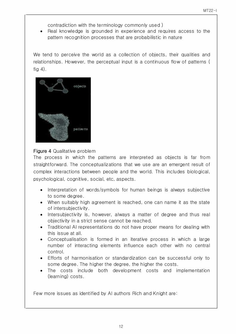
We tend to perceive the world as a collection of objects, their qualities and

relationships. However, the perceptual input is a continuous flow of patterns (

fig 4).

Figure 4 Qualitative problem

The process in which the patterns are interpreted as objects is far from

straightforward. The conceptualizations that we use are an emergent result of

complex interactions between people and the world. This includes biological,

psychological, cognitive, social, etc, aspects.

Interpretation of words/symbols for human beings is always subjective

to some degree.

When suitably high agreement is reached, one can name it as the state of intersubjectivity.

Intersubjectivity is, however, always a matter of degree and thus real

objectivity in a strict sense cannot be reached.

Traditional AI representations do not have proper means for dealing with

this issue at all.

Conceptualisation is formed in an iterative process in which a large

number of interacting elements influence each other with no central

control.

Efforts of harmonisation or standardization can be successful only to

some degree. The higher the degree, the higher the costs.

The costs include both development costs and implementation (learning) costs.

Few more issues as identified by AI authors Rich and Knight are:

MT22-I

13

Are any attributes of objects so basic that they occur in almost every

problem domain? If there are, we need to make sure that they are

handled appropriately in each of the mechanisms we propose.

Is there any important relationship that exists among attributes of

objects?

At what level should knowledge be represented? Is there a good set of

primitives into which all knowledge can be broken down? Is it helpful to use such primitives?

How should sets of objects be represented?

Given a large amount of knowledge stored in a database, how can

relevant parts be accessed when they are needed?

Evaluator’s Comments if any:

Question 2 What is Expert System?

Answer 2

An expert system is a software system that attempts to reproduce the

performance of one or more human experts, most commonly in a specific

problem domain, and is a traditional application and/or subfield of AI. A

wide variety of methods can be used to simulate the performance of the

expert, few important ones that are common to all such systems are:

1) The creation of a so-called “knowledgebase” which uses some

knowledge representation formalism to capture the subject matter

experts (SME) knowledge.

2) A process of gathering that knowledge from the SME and codifying it

accordingly to the formalism, which is called knowledge engineering.

Expert systems may or may not have learning components but a third

common element is that once a system is developed it is proven by

being placed in the same real world problem solving situation as the

human SME, typically as an aid to human workers or a supplement to

some information system.

MT22-I

14

An example of a typical Expert system is provided in following section.

In this example, we illustrate the reasoning process involved in an expert

system for a weather forecasting problem with special emphasis to its

architecture. An expert system consists of a knowledge base, database and

an inference engine for interpreting the database using the knowledge

supplied in the knowledge base. The reasoning process of a typical

illustrative expert system is described in Fig. 5. PR 1 in Fig. 5 represents i-

th production rule.

The inference engine attempts to match the antecedent clauses (IF parts) of

the rules with the data stored in the database. When all the antecedent

clauses of a rule are available in the database, the rule is fired, resulting in

new inferences. The resulting inferences are added to the database for

activating subsequent firing of other rules. In order to keep limited data in

the database, a few rules that contain an explicit consequent (THEN) clause

to delete specific data from the databases are employed in the knowledge

base. On firing of such rules, the unwanted data clauses as suggested by

the rule are deleted from the database. Here PR1 fires as both of its

antecedent clauses are present in the database. On firing of PR1, the

consequent clause “it-will-rain” will be added to the database for

subsequent firing of PR2.

Figure 5 Illustrative architecture of an expert system

Evaluator’s Comments if any:

MT22-I

15

Question 3 What do you understand by forward Vs backward reasoning?

Answer 3

Most of the common classical reasoning problems of AI can be solved by any

of the following two techniques called i) forward and ii) backward reasoning.

In a forward reasoning problem such as 4-puzzle games or the water-jug

problem, where the goal state is known, the problem solver has to identify the

states by which the goal can be reached. Such class of problems are generally

solved by expanding states from the known starting states with the help of a

domain-specific knowledge base. The generation of states from their

predecessor states may be continued until the goal is reached.

On the other hand, consider the problem of system diagnosis or driving a car

from an unknown place to home. Here, the problems can be easily solved by

employing backward reasoning, since the neighbouring states of the goal node

are known better than the neighbouring states of the starting states. For

example, in diagnosis problems, the measurement points are known better

than the cause of defects, while for the driving problem, the roads close to

home are known better than the roads close to the unknown starting location

of driving. It is thus clear that, whatever is the class of problems, system states

from starting state to goal or vice versa is to be identified, which requires

expanding one state to one or more states. If there is no knowledge to identify

the right offspring state from a given state, then many possible offspring states

are generated from a known state. This enhances the search-space for the

goal. When the distance (in arc length) between the starting state and goal

state is long, determining the intermediate states and the optimal path

(minimum arc length path) between the starting and the goal state becomes a

complex problem.

Given a set of rules like explained above, there are essentially two ways we can

use them to generate new knowledge:

1. Forward chaining: starts with the facts, and sees what rules apply (and

hence what should be done) given the facts. This is data driven.

2. Backward chaining: starts with something to find out, and looks for rules

that will help in answering it. This is goal driven.

MT22-I

16

Forward chaining:

In a forward chaining system ( Refer fig 6):

Facts are held in a working memory

Condition-action rules represent actions to take when specified facts

occur in working memory.

Typically the actions involve adding or deleting facts from working

memory.

Collect the rule whose condition matches a fact in WM. Do actions

indicated by the rule (add facts to WM or delete facts from WM)

If more than one rule matches Use conflict resolution strategy to

eliminate all but one

Repeat Until problem is solved or no condition match

Figure 6 Rule based system

Figure 7 A typical Forward Chaining example

Backward chaining:

Same rules/facts may be processed differently, using backward chaining

MT22-I

17

interpreter

Backward chaining means reasoning from goals back to facts. The idea

is that this focuses the search.

Uses checking hypothesis: Should I switch the sprinklers on?

To prove goal G: If G is in the initial facts, it is proven.

Otherwise, find a rule which can be used to conclude G, and try to prove

each of that rule’s conditions.

Figure 8 A typical backward chaining example

Evaluator’s Comments if any:

Question 4 Describe procedural Vs declarative knowledge?

Answer 4

The knowledge that goes into problem solving can be broadly classified into

MT22-I

18

three categories, viz., compiled knowledge, qualitative knowledge and

quantitative knowledge. Knowledge resulting from the experience of experts in

a domain, knowledge gathered from handbooks, old records, and standard

specifications etc., forms the compiled knowledge. Qualitative knowledge

consists of rules of thumb, approximate theories, causal models of processes

and common sense. Quantitative knowledge deals with techniques based on

mathematical theories, numerical techniques etc. Compiled as well as

qualitative knowledge can be further classified into two broad categories, viz.,

declarative knowledge and procedural knowledge. Declarative knowledge deals

with knowledge on physical properties of the problem domain, whereas

procedural knowledge deals with problem-solving techniques.

As per KSOU,

Declarative representation:

Static representation – knowledge about objects, events etc. and their

relationship and states given. This necessitates a program to know what to do with the knowledge and

how to do it.

Procedural representation:

Proceedings or control information needed to use the knowledge is

embedded in itself (knowledge), like how to find relevant facts...

This needs an interpreter to follow instructions specified in knowledge.

Knowledge encoded in some procedures and programs like the parser

has its inbuilt nouns, adjectives and verbs and will use them suitably.

Architectures with declarative representations have knowledge in a format that may be manipulated decomposed and analyzed by its reasoners. A classic

example of a declarative representation is logic. Advantages of declarative

knowledge are:

The ability to use knowledge in ways that the system designer did

not foresee

Architectures with procedural representations encode how to achieve a particular result. Advantages of procedural knowledge are:

Possibly faster usage

Often times, whether knowledge is viewed as declarative or procedural is not

MT22-I

19

an intrinsic property of the knowledge base, but is a function of what is

allowed to read from it.

A particular architecture may use both declarative and procedural knowledge at

different times, taking advantage of their different advantages. An example of

this is Atlantis, which has a low-level. The distinction between declarative and

procedural representations is somewhat artificial in that they may easily be

interconverted, depending on the type of processing that is done on them.

Evaluator’s Comments if any:

Question 5 Write a short note on Best first search?

Answer 5

Best first search depends on the use of heuristic to select most promising

paths to the goal node. Unlike hill climbing, however, this algorithm retains

all estimates computed for previously generated nodes and makes its

selections based on the best among them all. Thus at any point in the

search process, best first moves forward from the most promising of all the

nodes generated so far. In doing so, it avoids the potential traps

encountered in hill climbing.

The algorithm uses an evaluation function f (n) for each node to compute

estimate of "desirability" and expands most desirable unexpanded node.

• Evaluation function f (n) = h (n) (heuristic) = estimate of cost from n

to goal.

E.g., hSLD (n) = straight-line distance from n to desired goal.

In below example distance from Arad to Bucharest is estimated using the

lowest cost. At Arad 3 choices, Sibiu (253), Timisoara (329), Zerind (374).

Since Sibiu is least distance it is chosen. At Sibiu distance to Fagaras (176)

MT22-I

20

is least and it is selected. This continues till goal is reached.

Figure 9 Best first search

Algorithm:

1. Place the starting node s on the queue.

2. If the queue is empty, return failure and stop

3. If the first element on the queue is a goal node return success and

stop otherwise.

4. Remove the first element from the queue. Expand it and compute the

estimated goal distances for each child. Place the children on the

queue and arrange all queue elements in the ascending order

corresponding to goal distance from the front of the queue.

5. Return to step 2

Evaluator’s Comments if any:

Question 6 Explain with example traveling salesman problem?

Answer 6

The travelling salesman involves n cities with paths connecting the cities,

MT22-I

21

which begins with some starting city, visits each of the other cities exactly

once. He returns to the starting city. A typical tour is depicted in Figure 10

Typically a travelling salesperson will want to cover all the towns in their area

using the minimum driving distance.

The objective of a TSP is to find the minimal distance tour. To explore all such

tours requires an exponential amount of time. For examples a minimal solution

with only 10 cities is tractable, as an attempt to calculate for 20 c ities leads to

a worst case search of the order of 20! Tours.

Travelling salesperson problems tackle this by first turning the towns and roads

into a network.

We have seen that finding a tour that visits every arc (route inspection)

depended on earlier work by Euler. Similarly the problem of finding a tour that

visits every node (travelling salesperson) was investigated in the 19th Century

by the Irish mathematician Sir William Hamilton.

A Hamiltonian cycle is a tour which contains every node once.

Consider the Hamiltonian cycles for graph in Figure 11

There are just three essentially different Hamiltonian cycles:

Figure 10 Typical TSP tour

ABCDA with weight 17

ABDCA with weight 17

ACBDA with weight 16

MT22-I

22

Figure 11 Hamilton cycles

TSP is solved by selecting one of the optimal Hamilton cycles that make use of

least weight ACBDA with weight 16.

Evaluator’s Comments if any:

Question 7 Describe neural model?

Answer 7

The three classical models for an artificial neuron are described here.

McCulloch-Pitts Model

Figure 12 McCulloch-Pitts model of a neuron

MT22-I

23

In McCulloch-Pitts (MP) model figure 12 the activation (x) is given by a

weighted sum of its M input values (ai) and a bias term (θ). The output signal

(s) is typically a nonlinear function f(x) of the activation value x. The following

equations describe the operation of an MP model:

Three commonly used non linear functions (binary, ramp and sigmoid) are

shown in Figure 13, although only the binary function was used in the original

MP model.

Figure 13 Some non linear functions

Networks consisting of MP neurons with binary (on-off) outputs signals can be

configured to perform several logical functions. Figure 14 shows some

examples of logic circuits realized using the MP model.

MT22-I

24

Figure 14 Illustration of some elementary logic networks using MP neurons.

In this model a binary output function is used with the following logic:

f(x) = 1, x> 0

= 0, x≤ 0

A single input and a single output MP neuron with proper weight and threshold

gives an output a unit time later. This unit delay property of the MP neuron can

be used to build sequential digital circuits. With feedback, it is also possible to

have a memory cell which can retain the output indefinitely in the absence of

any input.

In the MP model the weights are fixed. Hence a network using this model does

not have the capability of learning. Moreover, the original model allows only

binary outputs states, operating at discrete time steps.

MT22-I

25

Perceptron:

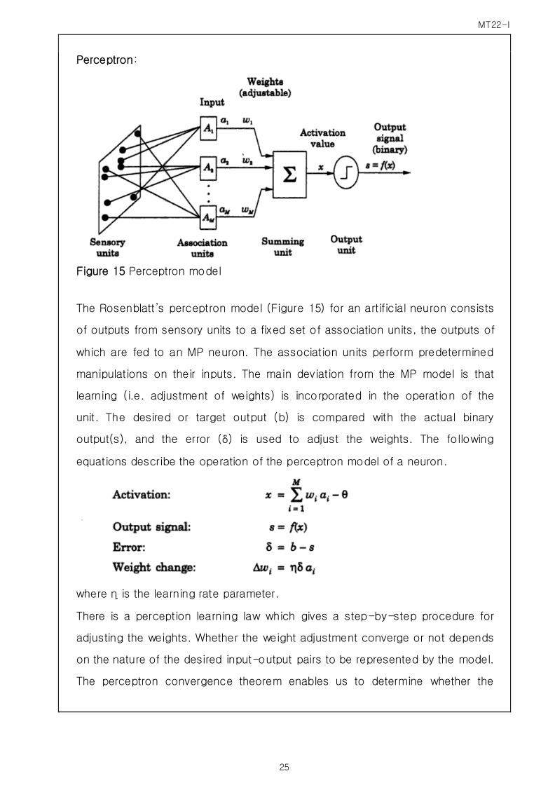
Figure 15 Perceptron model

The Rosenblatt’s perceptron model (Figure 15) for an artificial neuron consists

of outputs from sensory units to a fixed set of association units, the outputs of

which are fed to an MP neuron. The association units perform predetermined

manipulations on their inputs. The main deviation from the MP model is that

learning (i.e. adjustment of weights) is incorporated in the operation of the

unit. The desired or target output (b) is compared with the actual binary

output(s), and the error (δ) is used to adjust the weights. The following

equations describe the operation of the perceptron model of a neuron.

where η is the learning rate parameter.

There is a perception learning law which gives a step-by-step procedure for

adjusting the weights. Whether the weight adjustment converge or not depends

on the nature of the desired input-output pairs to be represented by the model.

The perceptron convergence theorem enables us to determine whether the

MT22-I

26

given pattern pairs are represent able or not. If the weights values converge,

then the corresponding problem is said to be represented by the perceptron

network.

Adaline:

Adaptive LINear Element (ADALINE) is a computing model proposed by Widrow

and is shown if Fig 15.

Figure 16 Widrow’s Adaline model of a neuron

The main distinction between the Rosenblatt’s perceptron model and the

Widrow’s Adaline model is that, in the Adaline the analog activation value (x) is

compared with the target output (b). In other words, the output is a linear

function of the activation value(x). The equations that describe the operation of

an Adaline are as follows:

Where η is the learning rate parameter. This weight update rule minimizes the

mean squared error δ2 , averaged over all inputs. Hence it is called Least Mean

Squared(LMS) error learning law. This law is derived using the negative

gradient of the error surface in the weight space. Hence it is also known as

gradient descent algorithm.

MT22-I

27

Evaluator’s Comments if any:

Question 8 Describe Pattern Recognition problem?

Answer 8

First let’s get a brief introduction to Pattern recognition and later define the

problem.

Pattern recognition is characteristic to all living organisms. However,

different creatures recognize differently. If a human would recognize another

human by sight, by voice or by handwriting, a dog may recognize a human

or other animal by smell thirty yards away which most humans are incapable

of doing. All of these examples are classified as recognition.

The object which is inspected for the "recognition" process is called a

pattern. Usually we refer to a pattern as a description of an object which we

want to recognize. In this text we are interested in spatial patterns like

humans, apples, fingerprints, electrocardiograms or chromosomes. In most

cases a pattern recognition problem is a problem of discriminating between

different populations. For example we may be interested among a thousand

humans to discriminate between four different types: (a) tall and thin (b) tall

and fat (c) short and thin (d) short and fat. We thus want to classify each

person in one of four populations. The recognition process thus turns into

classification. To determine which class the person belongs to, we must first

find which features are going to determine this classification. The age of the

person is clearly not a feature in this case. A reasonable choice of course is

the pair of numbers (height, weight) and we thus perform a feature selection

for this particular problem. Getting these measurements is called feature

extraction.

Clustering given input data is a major subject in pattern recognition. It

consists of dividing the data into clusters and establishing the cluster

centers and cluster boundaries. An a priori knowledge of the number of

clusters and their approximate locations definitely simplifies our task. We

then carry a supervised learning process. If the data is of no known

MT22-I

28

characteristic we obtain an unsupervised learning process.

Pattern recognition problem as defined by KSOU:

In any pattern recognition task we have a set of input patterns and the

corresponding output patterns. Depending on the nature of the output

patterns and the nature of the task environment, the problem could be

identified as one of association or classification or mapping. The given set

of input-output pattern pairs form only a few samples of an unknown

system. From these samples the pattern recognition model should capture

the characteristic of the system. Without looking into the details of the

system, let us assume that the input-output patterns are available or given to

us. Without loss of generality, let us alone assume that the patterns could be

represented as vectors in multidimensional spaces. We first state that the

most straightforward pattern recognition problem, namely, the pattern

association problem, and discuss its characteristic.

Pattern Association problem: Given a set of input-output pattern pairs(

a1,b1),( a2,b2),…( ai,bi),…,( al,bl) where al = ( al1,al2, ---,a1M) and bl = ( bl1,

bl2,…, bln) are M and N dimensional vectors, respectively, design a neural

network to associate each input pattern with the corresponding output

pattern.

If al, bl are distinct, then the problem is called heteroassociation. On the

other hand, if bl = al, then the problem is called autoassociaiton. In the latter

case the input and the corresponding output patterns refer to the same point

in an N-dimensional space, since M=N and ali =bli, I =1,2,…N, l=1,2,…, L.

The problem of storing the association of the input-output pattern pairs(

al,bl), l =1,2,…,L, involves determining the weights of a network to

accomplish the task. This is the training part. Once stored, the problem of

recall involves determining the output pattern for a given input pattern by

applying the operations of the network on the input pattern.

The recalled output pattern depends on the nature of the input and the

design of the network. If the input pattern is the same as one of those used

in the training, then the recalled output pattern is the same as the associated

pattern in the training. If the input pattern is a noisy version of the trained

input pattern, then the pattern may not be identical to any of the patterns

used in training the network. Let the input pattern is â = al + ε, where ε is a (

small amplitude) noise vector. Let us assume that â is closer( according to

MT22-I

29

some distance measure) to al than any other ak, k ≠ l. If the output of the

network for this input â is still bl, then the network is designed to exhibit an

accretive behavior. On the other hand, if the network produces an output b^

= bl+δ, such that | δ | -> 0 as | ε | -> 0, then the network is designed to

exhibit an interpolative behaviour. Depending on the interpretation of the

problem, several pattern recognition tasks can be viewed as variants of the

pattern association problem.

Evaluator’s Comments if any:

Question 9 Define simulated annealing?

Answer 9

In metallurgy, annealing is the process used to temper or harden metals and

glass by heating them to a high temperature and then gradually cooling them,

thus allowing the material to coalesce into a low-energy crystalline state. The

structural properties of a solid depend on the rate of cooling after the solid

has been heated beyond its melting point. If the solid is cooled slowly, large

crystals can be formed that are beneficial to the composition of the solid. If

the solid is cooled in a less controlled way, the result is a fragile solid with

undesirable properties. Annealing is to shake up the object at higher

temperatures so that the loose bonding of the molecules at that temperature

can be used to our advantage to give shape and reach the proper desired

goal state. In IT this has an analogous use to reach the desired best solution.

To understand simulated annealing, let's consider gradient descent (i.e.,

minimizing cost) and imagine the task of getting a ping-pong ball into the

deepest crevice in a bumpy surface. If we just let the ball roll, it will come to

rest at a local minimum. If we shake the surface, we can bounce the ball out

of the local minimum. The trick is to shake just hard enough to bounce the

MT22-I

30

ball out of local minima, but not hard enough to dislodge it from the global

minimum. The simulated annealing solution is to start by shaking hard (i.e., at

a high temperature) and then gradually reduce the intensity of the shaking

(i.e., lower the temperature).

The innermost loop of the simulated-annealing algorithm (Figure 17) is quite

similar to hill climbing. Instead of picking the best move, however, it picks a

random move. If the move improves the situation, it is always accepted.

Otherwise, the algorithm accepts the move with some probability less than 1.

The probability decreases exponentially with the "badness” of the move-the

amount ΔE by which the evaluation is worsened. The probability also

decreases as the "temperature" T goes down: "bad moves are more likely to

be allowed at the start when temperature is high, and they become more

unlikely as T decreases. One can prove that if the schedule lowers T slowly

enough, the algorithm will find a global optimum with probability approaching

1.

Simulated annealing was first used extensively to solve VLSl layout problems

in the early 1980s. It has been applied widely to factory scheduling and other

large-scale optimization tasks.

Figure 17 Simulated annealing search algorithm

A version of stochastic hill climbing where some downhill moves are allowed.

Downhill moves are accepted readily early in the annealing schedule and then

less often as time goes on. The Schedule input determines the value T as a

function of time.

MT22-I

31

Evaluator’s Comments if any:

Question 10 What is Boltzmann machine?

Answer 10

A Boltzmann machine (BM) is the name given to a type of simulated

stochastic recurrent neural network by Geofferey Hinton and Terry

Sejnowski.

Boltzmann machines can be seen as the stochastic, generative counterpart

of Hopfield nets. They were one of the first examples of a neural network

capable of learning internal representations, and are able to represent and

solve difficult combinatoric problems. However, due to a number of issues

discussed below, BM with un constrained connectivity has not proven useful

for practical problems in machine learning or inference. They are still

theoretically intriguing, however, due to the locality and hebbian nature of

their training algorithm, as well as their parallelism and the resemblance of

their dynamics to simple physical processes. If the connectivity is

constrained, the learning can be made efficient enough to be useful for

practical problems.

The BM is important because it is one of the first neural networks to

demonstrate learning of latent variables. BM learning was at first slow to

simulate, but the contrastive divergence algorithm of Geoff Hinton (year

2000) allows models such as BM to be trained much faster.

Structure of BM:

A BM like a Hopfield network, is a network of units with an “energy” defined

for the network. It also has binary units, but unlike Hopfield nets, BM units

are stochastic. The global energy, E, in a BM is identical in form to that of a

Hopfield network:

E = - Σ wij si sj + Σ θ i si

where

MT22-I

32

i <j

wij is the connection strength between unit j and unit i.

si is the state of unit i

θ i is the threshold of unit i.

The connections in a BM have two restrictions:

No unit has a connection with itself.

All connections are symmetric

Thus the difference in the global energy that results from a single unit I

being 0 versus 1, written ΔEi is given by:

ΔEi = Σ wij sj - θ i

A BM is made up of stochastic units. The probability, Pi of the ith unit being

on is given by:

Pi = 1 / (1 + exp (-1/T ΔEi)

Where the scalar T is referred to as the temperature of the system.

The network is run by repeatedly choosing a unit and setting its state

according to the above formula. After running for long enough at a certain

temperature, the probability of a global state of the network will depend only

upon the global state’s energy, according to a Boltzmann distribution. This

means that log-probabilities of global state become linear in their energies.

This relationship is true when the machine is at “thermal equilibrium”,

meaning that the probability distribution of global states has converged. If

we start running the network from a high temperature, and gradually

decrease it until we reach a thermal equilibrium at a low temperature, we are

guaranteed to converge to a distribution where the energy level fluctuates

around the global minimum. This process is simulated annealing.

Evaluator’s Comments if any: