mpc cep qin badgwell

Control Engineering Practice 11 (2003) 733–764

A survey of industrial model predictive control technology

S. Joe Qina,*, Thomas A. Badgwellb,1

aDepartment of Chemical Engineering, The University of Texas at Austin, 1 Texas Lonhorns, C0400, Austin, TX 78712, USAbAspen Technology, Inc., 1293 Eldridge Parkway, Houston, TX 77077, USA

Received 8 November 2001; accepted 31 August 2002

Abstract

This paper provides an overview of commercially available model predictive control (MPC) technology, both linear and

nonlinear, based primarily on data provided by MPC vendors. A brief history of industrial MPC technology is presented first,

followed by results of our vendor survey of MPC control and identification technology. A general MPC control algorithm is

presented, and approaches taken by each vendor for the different aspects of the calculation are described. Identification technology

is reviewed to determine similarities and differences between the various approaches. MPC applications performed by each vendor

are summarized by application area. The final section presents a vision of the next generation of MPC technology, with an emphasis

on potential business and research opportunities.

r 2002 Elsevier Science Ltd. All rights reserved.

1. Introduction

Model predictive control (MPC) refers to a class ofcomputer control algorithms that utilize an explicitprocess model to predict the future response of a plant.At each control interval an MPC algorithm attempts tooptimize future plant behavior by computing a sequenceof future manipulated variable adjustments. The firstinput in the optimal sequence is then sent into the plant,and the entire calculation is repeated at subsequentcontrol intervals. Originally developed to meet thespecialized control needs of power plants and petroleumrefineries, MPC technology can now be found in a widevariety of application areas including chemicals, foodprocessing, automotive, and aerospace applications.Several recent publications provide a good introduc-

tion to theoretical and practical issues associated withMPC technology. Rawlings (2000) provides an excellentintroductory tutorial aimed at control practitioners.Allgower, Badgwell, Qin, Rawlings, and Wright (1999)present a more comprehensive overview of nonlinearMPC and moving horizon estimation, includinga summary of recent theoretical developments and

numerical solution techniques. Mayne, Rawlings, Rao,and Scokaert (2000) provide a comprehensive review oftheoretical results on the closed-loop behavior of MPCalgorithms. Notable past reviews of MPC theory includethose of Garc!ıa, Prett, and Morari (1989); Ricker (1991);Morari and Lee (1991); Muske and Rawlings (1993),Rawlings, Meadows, and Muske (1994); Mayne (1997),and Lee and Cooley (1997). Several books on MPC haverecently been published (Allgower & Zheng, 2000;Kouvaritakis & Cannon, 2001; Maciejowski, 2002).The authors presented a survey of industrial MPC

technology based on linear models at the 1996 ChemicalProcess Control V Conference (Qin & Badgwell, 1997),summarizing applications through 1995. We presented areview of industrial MPC applications using nonlinearmodels at the 1998 Nonlinear Model Predictive Controlworkshop held in Ascona, Switzerland (Qin andBadgwell, 2000). Froisy (1994) and Kulhavy, Lu,and Samad (2001) describe industrial MPC practiceand future developments from the vendor’s viewpoint.Young, Bartusiak, and Fontaine (2001), Downs (2001),and Hillestad and Andersen (1994) report developmentof MPC technology within operating companies. Asurvey of MPC technology in Japan provides a wealth ofinformation on application issues from the point ofview of MPC users (Ohshima, Ohno, & Hashimoto,1995).

*Corresponding author. Tel.: +1-512-471-4417; fax: +1-512-471-

7060.

E-mail address: [email protected] (S.J. Qin).1At the time of the survey TAB was with Rice University.

0967-0661/02/$ - see front matter r 2002 Elsevier Science Ltd. All rights reserved.

PII: S 0 9 6 7 - 0 6 6 1 ( 0 2 ) 0 0 1 8 6 - 7

In recent years the MPC landscape has changeddrastically, with a large increase in the number ofreported applications, significant improvements intechnical capability, and mergers between several ofthe vendor companies. The primary purpose of thispaper is to present an updated, representative snapshotof commercially available MPC technology. The in-formation reported here was collected from vendorsstarting in mid-1999, reflecting the status of MPCpractice just prior to the new millennium, roughly 25years after the first applications.A brief history of MPC technology development is

presented first, followed by the results of our industrialsurvey. Significant features of each offering are outlinedand discussed. MPC applications to date by each vendorare then summarized by application area. The finalsection presents a view of next-generation MPCtechnology, emphasizing potential business and researchopportunities.

2. A brief history of industrial MPC

This section presents an abbreviated history ofindustrial MPC technology. Fig. 1 shows an evolution-ary tree for the most significant industrial MPCalgorithms, illustrating their connections in a conciseway. Control algorithms are emphasized here becauserelatively little information is available on the develop-ment of industrial identification technology. The follow-ing sub-sections describe key algorithms on the MPCevolutionary tree.

2.1. LQG

The development of modern control concepts can betraced to the work of Kalman et al. in the early 1960s(Kalman, 1960a, b). A greatly simplified description oftheir results will be presented here as a reference pointfor the discussion to come. In the discrete-time context,

the process considered by Kalman and co-workers canbe described by a discrete-time, linear state-space model:

xkþ1 ¼ Axk þ Buk þGwk; ð1aÞ

yk ¼ Cxk þ nk: ð1bÞ

The vector u represents process inputs, or manipulatedvariables, and vector y describes measured processoutputs. The vector x represents process states to becontrolled. The state disturbance wk and measurementnoise nk are independent Gaussian noise with zeromean. The initial state x0 is assumed to be Gaussianwith non-zero mean.The objective function F to be minimized

penalizes expected values of squared input and statedeviations from the origin and includes separate stateand input weight matrices Q and R to allow for tuningtrade-offs:

F ¼ EðJÞ; J ¼XN

j¼1

ðjjxkþj jj2Q þ jjukþj jj2RÞ: ð2Þ

The norm terms in the objective function are defined asfollows:

jjxjj2Q ¼ xTQx: ð3Þ

Implicit in this formulation is the assumption that allvariables are written in terms of deviations from adesired steady state. It was found that the solution tothis problem, known as the linear quadratic Gaussian

(LQG) controller, involves two separate steps. At timeinterval k; the output measurement yk is first used toobtain an optimal state estimate #xkjk:

#xkjk�1 ¼ A #xk�1jk�1 þ Buk�1; ð4aÞ

#xkjk ¼ #xkjk�1 þ Kf ðyk � C #xkjk�1Þ: ð4bÞ

Then the optimal input uk is computed using an optimalproportional state controller:

uk ¼ �Kc #xkjk: ð5Þ

LQG

IDCOM-M HIECON

SMCA

PCTPFC

IDCOM

SMOC

Connoisseur

DMC

DMC+

QDMC

RMPC

RMPCT

1960

1970

1980

1990

2000

1st generationMPC

2nd generationMPC

3rd generationMPC

4th generationMPC

Fig. 1. Approximate genealogy of linear MPC algorithms.

S.J. Qin, T.A. Badgwell / Control Engineering Practice 11 (2003) 733–764734

Here, the notation #xijj refers to the state estimate at timei given information up to and including time j: TheKalman filter gain Kf is computed from the solution of amatrix Ricatti equation. The controller gain Kc can befound by constructing a dual Ricatti equation, so thatthe same numerical techniques and software can be usedfor both calculations.The infinite prediction horizon of the LQG algorithm

endows the algorithm with powerful stabilizing proper-ties. For the case of a perfect model, it was shown to bestabilizing for any reasonable linear plant (stabilizableand the states are detectable through the quadraticcriterion) as long as Q is positive semidefinite and R ispositive definite.Extensions to handle practical issues such as control-

ling outputs, achieving offset-free control, and comput-ing the steady-state targets followed rapidly(Kwakernaak & Sivan, 1972). However, constraints onthe process inputs, states and outputs were generally notaddressed in the development of LQG theory.LQG theory soon became a standard approach to

solve control problems in a wide range of applicationareas. Goodwin, Graebe, and Salgado (2001) estimatethat there may be thousands of real-world applicationsof LQG with roughly 400 patents per year based on theKalman filter. However, it has had little impact oncontrol technology development in the process indus-tries. The most significant of the reasons cited for thisfailure include (Richalet, Rault, Testud, & Papon, 1976;Garc!ıa, Prett, & Morari, 1989):

* constraints;* process nonlinearities;* model uncertainty (robustness);* unique performance criteria;* cultural reasons (people, education, etc.).

It is well known that the economic operating point ofa typical process unit often lies at the intersection ofconstraints (Prett & Gillette, 1980). A successfulindustrial controller for the process industries musttherefore maintain the system as close as possible toconstraints without violating them. In addition, processunits are typically complex, nonlinear, constrainedmultivariable systems whose dynamic behavior changeswith time due to such effects as changes in operatingconditions and catalyst aging. Process units are alsoquite individual so that development of process modelsfrom fundamental physics and chemistry is difficult tojustify economically. Indeed, the application areaswhere LQG theory had a more immediate impact, suchas the aerospace industry, are characterized by physicalsystems for which it is technically and economicallyfeasible to develop accurate fundamental models.Process units may also have unique performance criteriathat are difficult to express in the LQG framework,

requiring time-dependent output weights or additionallogic to delineate different operating modes. However,the most significant reasons that LQG theory failed tohave a strong impact may have been related to theculture of the industrial process control community atthe time, in which instrument technicians and controlengineers either had no exposure to LQG concepts orregarded them as impractical.This environment led to the development, in industry,

of a more general model based control methodology inwhich the dynamic optimization problem is solved on-line at each control execution. Process inputs arecomputed so as to optimize future plant behavior overa time interval known as the prediction horizon. In thegeneral case any desired objective function can be used.Plant dynamics are described by an explicit processmodel which can take, in principle, any requiredmathematical form. Process input and output con-straints are included directly in the problem formulationso that future constraint violations are anticipatedand prevented. The first input of the optimalinput sequence is injected into the plant and the problemis solved again at the next time interval usingupdated process measurements. In addition todeveloping more flexible control technology, newprocess identification technology was developed to allowquick estimation of empirical dynamic models from testdata, substantially reducing the cost of model develop-ment. This new methodology for industrial processmodeling and control is what we now refer to as MPCtechnology.In modern processing plants the MPC controller is

part of a multi-level hierarchy of control functions. Thisis illustrated in Fig. 2, which shows a conventionalcontrol structure on the left for Unit 1 and a MPCstructure on the right for Unit 2. Similar hierarchicalstructures have been described by Richalet, Rault,Testud, and Papon (1978) and Prett and Garc!ıa(1988). At the top of the structure a plant-wideoptimizer determines optimal steady-state settings foreach unit in the plant. These may be sent to localoptimizers at each unit which run more frequently orconsider a more detailed unit model than is possible atthe plant-wide level. The unit optimizer computes anoptimal economic steady state and passes this to thedynamic constraint control system for implementation.The dynamic constraint control must move the plantfrom one constrained steady state to another whileminimizing constraint violations along the way. In theconventional structure this is accomplished by using acombination of PID algorithms, lead-lag (L/L) blocksand high/low select logic. It is often difficult to translatethe control requirements at this level into an appropriateconventional control structure. In the MPC methodol-ogy this combination of blocks is replaced by a singleMPC controller.

S.J. Qin, T.A. Badgwell / Control Engineering Practice 11 (2003) 733–764 735

Although the development and application of MPCtechnology was driven by industry, it should be notedthat the idea of controlling a system by solving asequence of open-loop dynamic optimization problemswas not new. Propoi (1963), for example, described amoving horizon controller. Lee and Markus (1967)anticipated current MPC practice in their 1967 optimalcontrol text:

One technique for obtaining a feedback controllersynthesis from knowledge of open-loop controllers isto measure the current control process state andthen compute very rapidly for the open-loopcontrol function. The first portion of this func-tion is then used during a short time interval, afterwhich a new measurement of the function iscomputed for this new measurement. The procedureis then repeated.

There is, however, a wide gap between theoryand practice. The essential contribution of industrywas to put these ideas into practice on operatingunits. Out of this experience came a fresh set ofproblems that has kept theoreticians busy ever since.

2.2. IDCOM

The first description of MPC control applications waspresented by Richalet et al. in 1976 Conference (Richaletet al., 1976) and later summarized in 1978 Automatica

paper (Richalet et al., 1978). They described theirapproach as model predictive heuristic control (MPHC).The solution software was referred to as IDCOM, anacronym for Identification and Command. The distin-guishing features of the IDCOM approach are:

* impulse response model for the plant, linear in inputsor internal variables;

* quadratic performance objective over a finite predic-tion horizon;

* future plant output behavior specified by a referencetrajectory;

* input and output constraints included in the for-mulation;

* optimal inputs computed using a heuristic iterativealgorithm, interpreted as the dual of identification.

Richalet et al. chose an input–output representationof the process in which the process inputs influence theprocess outputs directly. Process inputs are divided into

(every second)

FC PC TC LC FC PC TC LC

Plant-Wide Optimization

Unit 1 Local Optimizer Unit 2 Local Optimizer

High/Low Select Logic

PID L/L PID

SUM SUM

Unit 1 - ConventionalControl Structure

Unit 2 - Model PredictiveControl Structure

Global EconomicOptimization

Local EconomicOptimization(every hour)

(every minute)ControlConstraintDynamic

(MPC)Model Predictive Control

Unit 1 DCS- PID Controls Unit 2 DCS-PID Controls ControlBasic Dynamic

(every day)

Fig. 2. Hierarchy of control system functions in a typical processing plant. Conventional structure is shown at the left; MPC structure is shown at the

right.


manipulated variables (MVs) which the controlleradjusts, and disturbance variables (DVS) which arenot available for control. Process outputs are referred toas controlled variables (CVs). They chose to describe therelationship between process inputs and outputs using adiscrete-time finite impulse response (FIR) model. Forthe single input, single output (SISO) case the FIRmodel looks like:

ykþj ¼XN

i¼1

hiukþj�i: ð6Þ

This model predicts that the output at a given timedepends on a linear combination of past input values;the summation weights hi are the impulse responsecoefficients. The sum is truncated at the point wherepast inputs no longer influence the output; thisrepresentation is therefore only possible for stableplants.The finite impulse response was identified from plant

test data using an algorithm designed to minimize thedistance between the plant and model impulse responsesin parameter space. The control problem was solvedusing the same algorithm by noting that control is themathematical dual of identification. The iterative natureof the control algorithm allows input and outputconstraints to be checked as the algorithm proceeds toa solution. Because the control law is not linear andcould not be expressed as a transfer function, Richaletet al. refer to it as heuristic. In today’s context thealgorithm would be referred to as a linear MPCcontroller.The MPHC algorithm drives the predicted future

output trajectory as closely as possible to a referencetrajectory, defined as a first order path from the currentoutput value to the desired setpoint. The speed of thedesired closed-loop response is set by the time constantof the reference trajectory. This is important in practicebecause it provides a natural way to control theaggressiveness of the algorithm; increasing the timeconstant leads to a slower but more robust controller.Richalet et al. make the important point that dynamic

control must be embedded in a hierarchy of plantcontrol functions in order to be effective. They describefour levels of control, very similar to the structureshown in Fig. 2:

* Level 3—Time and space scheduling of production.* Level 2—Optimization of setpoints to minimize costs

and ensure quality and quantity of production.* Level 1—Dynamic multivariable control of the plant.* Level 0—Control of ancillary systems; PID control of

valves.

They point out that significant benefits do not comefrom simply reducing the variations of a controlledvariable through better dynamic control at level 1. The

real economic benefits come at level 2 where betterdynamic control allows the controlled variable setpointto be moved closer to a constraint without violating it.This argument provides the basic economic motivationfor using MPC technology. This concept of a hierarchyof control functions is fundamental to advanced controlapplications and seems to have been followed by manypractitioners. Prett and Garc!ıa (1988), for example,describe a very similar hierarchy.Richalet et al. describe applications of the MPHC

algorithm to a fluid catalytic cracking unit (FCCU)main fractionator column, a power plant steam gen-erator and a poly-vinyl chloride (PVC) plant. All ofthese examples are constrained multivariable pro-cesses. The main fractionator example involvedcontrolling key tray temperatures to stabilize thecomposition of heavy and light product streams. Thecontroller adjusted product flowrates to compensatefor inlet temperature disturbances and to maintainthe level of a key internal tray. The power plantsteam generator problem involved controlling thetemperature and pressure of steam delivered to theturbine. This application is interesting becausethe process response time varied inversely with load onthe system. This nonlinearity was overcome byexecuting the controller with a variable sample time.Benefits for the main fractionator application werereported as $150; 000=yr; due to increasing the flowrateof the light product stream. Combined energy savingsfrom two columns in the PVC plant were reported as$220; 000=yr:

2.3. DMC

Engineers at Shell Oil developed their own indepen-dent MPC technology in the early 1970s, with an initialapplication in 1973. Cutler and Ramaker presenteddetails of an unconstrained multivariable control algo-rithm which they named dynamic matrix control (DMC)at the 1979 National AIChE meeting (Cutler & Ra-maker, 1979) and at the 1980 Joint Automatic ControlConference (Cutler & Ramaker, 1980). In a companionpaper at the 1980 meeting Prett and Gillette (1980)described an application of DMC technology to anFCCU reactor/regenerator in which the algorithm wasmodified to handle nonlinearities and constraints.Neither paper discussed their process identificationtechnology. Key features of the DMC control algorithminclude:

* linear step response model for the plant;* quadratic performance objective over a finite predic-

tion horizon;* future plant output behavior specified by trying to

follow the setpoint as closely as possible;


* optimal inputs computed as the solution to a least-squares problem.

The linear step response model used by the DMCalgorithm relates changes in a process output to aweighted sum of past input changes, referred to as inputmoves. For the SISO case the step response model lookslike:

ykþj ¼XN�1

i¼1

si Dukþj�i þ sNukþj�N : ð7Þ

The move weights si are the step response coefficients.Mathematically the step response can be defined as theintegral of the impulse response; given one model formthe other can be easily obtained. Multiple outputs werehandled by superposition. By using the step responsemodel one can write predicted future output changes asa linear combination of future input moves. The matrixthat ties the two together is the so-called Dynamic

Matrix. Using this representation allows the optimalmove vector to be computed analytically as the solutionto a least-squares problem. Feedforward control isreadily included in this formulation by modifying thepredicted future outputs. In practice the required matrixinverse can be computed off-line to save computation.Only the first row of the final controller gain matrixneeds to be stored because only the first move needs tobe computed.The objective of a DMC controller is to drive the

output as close to the setpoint as possible in a least-squares sense with a penalty term on the MV moves.This results in smaller computed input moves and a lessaggressive output response. As with the IDCOMreference trajectory, this technique provides a degreeof robustness to model error. Move suppression factorsalso provide an important numerical benefit in that theycan be used to directly improve the conditioning of thenumerical solution.Cutler and Ramaker showed results from a furnace

temperature control application to demonstrate im-proved control quality using the DMC algorithm.Feedforward response of the DMC algorithm to inlettemperature changes was superior to that of a conven-tional PID lead/lag compensator.In their paper Prett and Gillette (1980) described an

application of DMC technology to FCCU reactor/regenerator control. Four such applications werealready completed and two additional applications wereunderway at the time the paper was written. Prett andGillette described additional modifications to the DMCalgorithm to prevent violation of absolute inputconstraints. When a predicted future input camesufficiently close to an absolute constraint, an extraequation was added to the process model that woulddrive the input back into the feasible region. These werereferred to as time variant constraints. Because the

decision to add the equation had to be made on-line, thematrix inverse solution had to be recomputed at eachcontrol execution. Prett and Gillette developed a matrixtearing solution in which the original matrix inversecould be computed off-line, requiring only the matrixinverse corresponding to active time variant constraintsto be computed on-line.The initial IDCOM and DMC algorithms represent

the first generation of MPC technology; they had anenormous impact on industrial process control andserved to define the industrial MPC paradigm.

2.4. QDMC

The original IDCOM and DMC algorithms providedexcellent control of unconstrained multivariable pro-cesses. Constraint handling, however, was still some-what ad hoc. Engineers at Shell Oil addressed thisweakness by posing the DMC algorithm as a quadraticprogram (QP) in which input and output constraintsappear explicitly. Cutler et al. first described the QDMCalgorithm in a 1983 AIChE conference paper (Cutler,Morshedi, & Haydel, 1983). Garc!ıa and Morshedi(1986) published a more comprehensive descriptionseveral years later.Key features of the QDMC algorithm include:

* linear step response model for the plant;* quadratic performance objective over a finite predic-

tion horizon;* future plant output behavior specified by trying to

follow the setpoint as closely as possible subject to amove suppression term;

* optimal inputs computed as the solution to aquadratic program.

Garc!ıa and Morshedi show how the DMC objectivefunction can be re-written in the form of a standard QP.Future projected outputs can be related directly back tothe input move vector through the dynamic matrix; thisallows all input and output constraints to be collectedinto a matrix inequality involving the input move vector.Although the QDMC algorithm is a somewhat ad-vanced control algorithm, the QP itself is one of thesimplest possible optimization problems that one couldpose. The Hessian of the QP is positive definite for linearplants and so the resulting optimization problem isconvex. This means that a solution can be found readilyusing standard commercial optimization codes.Garc!ıa and Morshedi wrapped up their paper by

presenting results from a pyrolysis furnace application.The QDMC controller adjusted fuel gas pressure inthree burners in order to control stream temperature atthree locations in the furnace. Their test resultsdemonstrated dynamic enforcement of input constraintsand decoupling of the temperature dynamics. They


reported good results on many applications within Shellon problems as large as 12� 12 (12 process outputs and12 process inputs). They stated that above all, theQDMC algorithm had proven particularly profitable inan on-line optimization environment, providing asmooth transition from one constrained operating pointto another.The QDMC algorithm can be regarded as represent-

ing a second generation of MPC technology, comprisedof algorithms which provide a systematic way toimplement input and output constraints. This wasaccomplished by posing the MPC problem as a QP,with the solution provided by standard QP codes.

2.5. IDCOM-M, HIECON, SMCA, and SMOC

As MPC technology gained wider acceptance, andproblems tackled by MPC technology grew larger andmore complex, control engineers implementing secondgeneration MPC technology ran into other practicalproblems. The QDMC algorithm provided a systematicapproach to incorporate hard input and output con-straints, but there was no clear way to handle aninfeasible solution. For example it is possible for afeedforward disturbance to lead to an infeasible QP;what should the control do to recover from infeasibility?The soft constraint formulation is not completelysatisfactory because it means that all constraints willbe violated to some extent, as determined by the relativeweights. Clearly some output constraints are moreimportant than others, however, and should never beviolated. Would not it make sense then to shed lowpriority constraints in order to satisfy higher priority ones?In practice, process inputs and outputs can be lost in

real time due to signal hardware failure, valve saturationor direct operator intervention. They can just as easilycome back into the control problem at any sampleinterval. This means that the structure of the problemand the degrees of freedom available to the control canchange dynamically. This is illustrated in Fig. 3, whichillustrates the shape of the process transfer function

matrix for three general cases. The square plant case,which occurs when the plant has just as many MVs asCVs, leads to a control problem with a unique solution.In the real world, square is rare. More common is the fat

plant case, in which there are more MVs available thanthere are CVs to control. The extra degrees of freedomavailable in this case can be put to use for additionalobjectives, such as moving the plant closer to an optimaloperating point. When valves become saturated or lowerlevel control action is lost, the plant may reach acondition in which there are more CVs than MVs; this isthe thin plant case. In this situation it will not be possibleto meet all of the control objectives; the controlspecifications must be relaxed somehow, for exampleby minimizing CV violations in a least-squared sense.Fault tolerance is also an important practical issue.

Rather than simply turning itself off as signals are lost, apractical MPC controller should remain online and tryto make the best of the sub-plant under its control. Amajor barrier to achieving this goal is that a wellconditioned multivariable plant may contain a numberof poorly conditioned sub-plants. In practice an MPCcontroller must recognize and screen out poorly condi-tioned sub-plants before they result in erratic controlaction.It also became increasingly difficult to translate

control requirements into relative weights for a singleobjective function. Including all the required trade-offsin a single objective function means that relative weightshave to be assigned to the value of output setpointviolations, output soft constraint violations, inputsmoves, and optimal input target violations. For largeproblems it is not easy to translate control specificationsinto a consistent set of relative weights. In some cases itdoes not make sense to include these variables in thesame objective function; driving the inputs to theiroptimal targets may lead to larger violation of output softconstraints, for example. Even when a consistent set ofrelative weights can be found, care must be taken to avoidscaling problems that lead to an ill-conditioned solution.Prett and Garc!ıa (1988) commented on this problem:

CV's

MV's

SquarePlant

CV's Fat Plant

MV's

Over-determined

CV's

MV's

degrees of freedom < 0

PlantThin

degrees of freedom = 0Unique solution

degrees of freedom > 0Under-determined

Fig. 3. Process structure determines the degrees of freedom available to the controller. Adapted from Froisy (1994).


oscar

Realce

oscar

Realce

The combination of multiple objectives into oneobjective (function) does not allow the designer toreflect the true performance requirements.

These issues motivated engineers at Adersa, Setpoint,Inc., and Shell (France) to develop new versions of MPCalgorithms. The version marketed by Setpoint was calledIDCOM-M (the M was to distinguish this from a singleinput/single output version called IDCOM-S), while thenearly identical Adersa version was referred to ashierarchical constraint control (HIECON). The ID-COM-M controller was first described in a paper byGrosdidier, Froisy, and Hammann (1988). A secondpaper presented at the 1990 AIChE conference describesan application of IDCOM-M to the Shell FundamentalControl Problem (Froisy & Matsko, 1990) and providesadditional details concerning the constraint methodo-logy. Distinguishing features of the IDCOM-M algo-rithm include:

* linear impulse response model of plant;* controllability supervisor to screen out ill-condi-

tioned plant subsets;* multi-objective function formulation; quadratic out-

put objective followed by a quadratic input objective;* controls a subset of future points in time for each

output, called the coincidence points, chosen from areference trajectory;

* a single move is computed for each input;* constraints can be hard or soft, with hard constraints

ranked in order of priority.

An important distinction of the IDCOM-M algorithmis that it uses two separate objective functions, one for theoutputs and then, if there are extra degrees of freedom,one for the inputs. A quadratic output objectivefunction is minimized first subject to hard inputconstraints. Each output is driven as closely as possibleto a desired value at a single point in time known as thecoincidence point. The name comes from the fact thatthis is where the desired and predicted values shouldcoincide. The desired output value comes from a firstorder reference trajectory that starts at the currentmeasured value and leads smoothly to the setpoint.Each output has two basic tuning parameters; acoincidence point and a closed-loop response time, usedto define the reference trajectory.Grosdidier et al. (1988) provide simulation results for

a representative FCCU regenerator control problem.The problem involves controlling flue gas composition,flue gas temperature, and regenerator bed temperatureby manipulating feed oil flow, recycle oil flow and air tothe regenerator. The first simulation example demon-strates how using multiple inputs can improve dynamicperformance while reaching a pre-determined optimalsteady-state condition. A second example demonstrateshow the controller switches from controlling one output

to controlling another when a measured disturbancecauses a constraint violation. A third example demon-strates the need for the controllability supervisor. Whenan oxygen analyzer fails, the controllability supervisor isleft with only flue gas temperature and regenerator bedtemperature to consider. It correctly detects that control-ling both would lead to an ill-conditioned problem; this isbecause these outputs respond in a very similar way tothe inputs. Based on a pre-set priority it elects to controlonly the flue gas temperature. When the controllabilitysupervisor is turned off the same simulation scenarioleads to erratic and unacceptable input adjustments.Setpoint engineers continued to improve the IDCOM-

M technology, and eventually combined their identifica-tion, simulation, configuration, and control productsinto a single integrated offering called SMCA, forSetpoint Multivariable Control Architecture. An im-proved numerical solution engine allowed them to solvea sequence of separate steady-state target optimizations,providing a natural way to incorporate multiple rankedcontrol objectives and constraints.In the late 1980’s engineers at Shell Research in

France developed the Shell Multivariable OptimizingController (SMOC) (Marquis & Broustail, 1998; Yousfi& Tournier, 1991) which they described as a bridgebetween state-space and MPC algorithms. They soughtto combine the constraint handling features of MPCwith the richer framework for feedback offered by state-space methods. To motivate this effort they discussedthe control of a hydrotreater unit with four reactor bedsin series. The control system must maintain average bedtemperature at a desired setpoint and hold temperaturedifferences between the beds close to a desired profile,while preventing violation of maximum temperaturelimits within each reactor. Manipulated variablesinclude the first reactor inlet temperature and quenchflows between the beds. A typical MPC input/outputmodel would view the manipulated variables as inputsand the bed temperatures as independent outputs, and aconstant output disturbance would be assigned to eachbed temperature. But it is clear that the bed tempera-tures are not independent, in that a disturbance in thefirst bed will ultimately affect all three downstreamreactors. In addition, the controlled variables are not theprocess outputs but rather linear combinations thereof.State-space control design methods offer a naturalsolution to these problems but they do not provide anoptimal way to enforce maximum bed temperatureconstraints.The SMOC algorithm includes several features that

are now considered essential to a ‘‘modern’’ MPCformulation:

* State-space models are used so that the full range oflinear dynamics can be represented (stable, unstable,and integrating).


* An explicit disturbance model describes the effect ofunmeasured disturbances; the constant output dis-turbance is simply a special case.

* A Kalman filter is used to estimate the plant statesand unmeasured disturbances from output measure-ments.

* A distinction is introduced between controlled vari-

ables appearing in the control objective and feedback

variables that are used for state estimation.* Input and output constraints are enforced via a QP

formulation.

The SMOC algorithm is nearly equivalent to solvingthe LQR problem with input and output constraints,except that it is still formulated on a finite horizon. Assuch, it does not inherit the strong stabilizing propertiesof the LQR algorithm. A stabilizing, infinite-horizonformulation of the constrained LQR algorithm wouldcome only after academics began to embrace the MPCparadigm in the 1990s (Rawlings & Muske, 1993;Scokaert & Rawlings, 1998).The IDCOM-M, HIECON, SMCA, and SMOC

algorithms represent a third generation of MPC techno-logy; others include the PCT algorithm sold by Profi-matics, and the RMPC algorithm sold by Honeywell.This generation distinguishes between several levels ofconstraints (hard, soft, ranked), provides some mecha-nism to recover from an infeasible solution, addressesthe issues resulting from a control structure that changesin real time, provides a richer set of options forfeedback, and allows for a wider range of process dyna-mics (stable, integrating and unstable) and controllerspecifications.

2.6. DMC-plus and RMPCT

In the last 5 years, increased competition and themergers of several MPC vendors have led to significantchanges in the industrial MPC landscape. In late 1995Honeywell purchased Profimatics, Inc. and formedHoneywell Hi-Spec Solutions. The RMPC algorithmoffered by Honeywell was merged with the ProfimaticsPCT controller to create their current offering calledRMPCT. In early 1996, Aspen Technology Inc.purchased both Setpoint, Inc. and DMC Corporation.This was followed by acquisition of Treiber Controls in1998. The SMCA and DMC technologies were subse-quently merged to create Aspen Technology’s currentDMC-plus product. DMC-plus and RMPCT arerepresentative of the fourth generation MPC technologysold today, with features such as:

* Windows-based graphical user interfaces.* Multiple optimization levels to address prioritized

control objectives.

* Additional flexibility in the steady-state target opti-mization, including QP and economic objectives.

* Direct consideration of model uncertainty (robustcontrol design).

* Improved identification technology based on predic-tion error method and sub-space ID methods.

These and other MPC algorithms currently available inthe marketplace are described in greater detail in thenext section.

3. Survey of MPC technology products

The industrial MPC technology has changed con-siderably since the publication of our first survey 5 yearsago (Qin & Badgwell, 1996), which included data fromfive vendors: Adersa, DMC, Honeywell, Setpoint, andTreiber Controls. In late 1995 Honeywell purchasedProfimatics and formed Honeywell Hi-Spec. In early1996, Setpoint and DMC were both acquired by AspenTechnology. Two years later Aspen purchased TreiberControls so that three of the companies in our originalsurvey had merged into one. These mergers, continuedproduct development, and the emergence of viablenonlinear MPC products (Qin & Badgwell, 1998)changed the MPC market enough for us to believe thatan updated survey would be worthwhile.We began collecting data for the present survey in

mid-1999, when we solicited information from eightvendors in order to assess the current status ofcommercial MPC technology. The companies surveyedand their product names and descriptions are listed inTables 1 and 2. In this survey we added two newcompanies offering linear MPC products: Shell GlobalSolutions (SGS) and Invensys Systems, Inc. (ISI) (Lewis,Evans, & Sandoz, 1991) in the UK. Three nonlinearMPC vendors were also included: Continental Controls,

Table 1

Companies and products included in Linear MPC technology survey

Company Product name Description

Adersa HIECON Hierarchical constraint control

PFC Predictive functional control

GLIDE Identification package

Aspen Tech DMC-plus Dynamic matrix control package

DMC-plus

model

Identification package

Honeywell RMPCT Robust model predictive control

Hi-Spec technology

Shell Global

Solutions

SMOC-IIa Shell multivariable optimizing control

Invensys Connoisseur Control and identification package

aSMOC-I was licensed to MDC Technology and Yokogawa in the

past. Shell global solutions is the organization that markets the current

SMOC technology.


DOT Products, and Pavilion Technologies. We believethat the technology sold by these companies isrepresentative of the industrial state of the art; we fullyrecognize that we have omitted some MPC vendorsfrom our survey, especially those who just entered themarket (e.g., Fisher-Rosemount, ABB). Some compa-nies were not asked to participate, some chose not toparticipate, and some responded too late to be includedin the paper. Only companies which have documentedsuccessful MPC applications were asked to participate.It should be noted that several companies make use of

MPC technology developed in-house but were notincluded in the survey because they do not offer theirtechnology externally. These MPC packages are eitherwell known to academic researchers or not known at allfor proprietary reasons. The SMOC algorithm originallydeveloped at Shell France is included in this surveybecause it is now commercially available through SGS.MDC Technology, Inc. and Yokogawa had licenseagreements with Shell.Initial data in this survey were collected from

industrial MPC vendors using a written survey. Blankcopies of the survey form are available upon requestfrom the authors. Survey information was supplementedby published papers, product literature (DMC Corp.,1994; Setpoint Inc., 1993; Honeywell Inc., 1995), andpersonal communication between the authors and

vendor representatives. Results of the linear MPCsurvey are summarized in Tables 3, 4 and 6. NonlinearMPC survey results are summarized separately in Tables5 and 7. While the data are provided by the vendors, theanalysis is that of the authors. In presenting the surveyresults our intention is to highlight the importantfeatures of each algorithm; it is not our intent todetermine the superiority of one product versus another.The purpose of showing the application numbers is togive a relative magnitude on how MPC is applied todifferent areas. The absolute numbers are not veryimportant as they are changing fast. The numbers arenot exactly comparable as the size of each MPCapplication can be very different. With this under-standing in mind, we first discuss the overall procedurefor control design and tuning. Then we describe thevarious model forms used for both the linear andnonlinear technology. The last two sections summarizethe main features of the identification and controlproducts sold by each vendor.

3.1. Control design and tuning

The MPC control design and tuning procedure isgenerally described as follows (DMC Corp., 1994;Setpoint Inc., 1993; Honeywell Inc., 1995):

* From the stated control objectives, define the size ofthe problem, and determine the relevant CVs, MVs,and DVs.

* Test the plant systematically by varying MVs andDVs; capture and store the real-time data showinghow the CVs respond.

* Derive a dynamic model either from first-principlesor from the plant test data using an identificationpackage.

* Configure the MPC controller and enter initial tuningparameters.

* Test the controller off-line using closed-loop simula-tion to verify the controller performance.

Table 2

Companies and products included in Nonlinear MPC technology

survey

Company Product name Description

Adersa PFC Predictive functional

control

Aspen Tech Aspen Target Nonlinear MPC package

Continental Controls,

Inc.

MVC Multivariable control

DOT Products NOVA-NLC NOVA nonlinear

controller

Pavilion Technologies Process Perfecter Nonlinear control

Table 3

Comparison of linear MPC identification technology

Product Test protocol Model forma Est. methodb Uncert. bound

DMC-plus step, PRBS VFIR, LSS MLS Yes

RMPCTc PRBS, step FIR, ARX, BJ LS, GN, PEM Yes

AIDAd PRBS, step LSS, FIR, TF, MM PEM-LS, GN Yes

Glide non-PRBS TF GD, GN, GM Yes

Connoisseur PRBS, step FIR, ARX, MM RLS, PEM Yes

aModel Form: finite impulse response (FIR), velocity FIR (VFIR), Laplace transfer function (TF), linear state-space (LSS), auto-regressive with

exogenous input (ARX), Box–Jenkins (BJ), multi-model (MM).bEst. method: least-squares (LS), modified LS (MLS), recursive LS (RLS), subspace ID (SMI), Gauss–Newton (GN), prediction error method

(PEM), gradient descent (GD), global method (GM).cThe commercial name for RMPCT is profit-controller.dAIDA: advanced identification data analysis.


* Download the configured controller to the destina-tion machine and test the model predictions in open-

loop mode.* Close the loop and refine the tuning as needed.

All of the MPC packages surveyed here providesoftware tools to help with the control design, modeldevelopment, and closed-loop simulation steps. Asignificant amount of time is currently spent at theclosed-loop simulation step to verify acceptable perfor-mance and robustness of the control system. Typically,tests are performed to check the regulatory and servoresponse of each CV, and system response to violationsof major constraints is verified. The final tuning is thentested for sensitivity to model mismatch by varying thegain and dynamics of key process models. However,even the most thorough simulation testing usuallycannot exhaust all possible scenarios.Of the products surveyed here, only the RMPCT

package provides robust tuning in an automatic way.This is accomplished using a min–max design procedurein which the user enters estimates of model uncertainty

directly. Tuning parameters are computed to optimizeperformance for the worst case model mismatch.Robustness checks for the other MPC controllers areperformed by closed-loop simulation.

3.2. Process models

The technical scope of an MPC product is largelydefined by the form of process model that it uses. Tables3 and 5 show that a wide variety of linear and nonlinearmodel forms are used in industrial MPC algorithms. It ishelpful to visualize these models in a two-dimensionalspace, as illustrated in Fig. 4. The horizontal axis refersto the source of information used for model develop-ment, and the vertical axis designates whether the modelis linear or nonlinear. The far left side of the diagramrepresents empirical models that are derived exclusivelyfrom process test data. Because empirical models mainlyperform fitting between the points of a data set, theygenerally cannot be expected to accurately predictprocess behavior beyond the range of the test data usedto develop them. At the far right side of the diagram lie

Table 4

Comparison of linear MPC control technology

Company Aspen Honeywell Adersa Adersa Invensys SGS

Tech Hi-Spec

Product DMC-plus RMPCT HIECON PFC Connois. SMOC

Linear Model FSR ARX, TF FIR LSS,TF,ARX ARX,FIR LSS

Formsa L,S,I,U L,S,I,U L,S,I L,N,S,I,U L,S,I,U L,S,I,U

Feedbackb CD, ID CD, ID CD, ID CD, ID CD, ID KF

Rem Ill-condc IMS SVT — — IMS IMS

SS Opt Objd L=Q½I;O;y;R Q[I,O] — Q[I,O] L[I,O] Q[I,O],R

SS Opt Conste IH,OS,R IH,OH — IH,OH IH,OH IH,OS

Dyn Opt Objf Q[I,O,M],S Q[I,O] Q[O],Q[I] Q[I,O],S Q[I,O,M] Q[I,O]

Dyn Opt Constg IH IH,OS IH,OH,OS,R IA,OH,OS,R IH,OS,R IH,OS

Output Trajh S,Z S,Z,F S,Z,RT S,Z,RT S,Z S,Z,RTB,F

Output Horizi FH FH FH CP FH FH

Input Paramj MMB MM SM BF MMB MMB

Sol. Methodk SLS ASQP ASQP LS ASQP ASQP

References Cutler and Ramaker (1979)

and DMC Corp., (1994)

Honeywell

Inc., (1995)

Richalet

(1993)

Richalet (1993) Marquis and

Broustail (1998)

aModel form: Finite impulse response (FIR), finite step response (FSR), Laplace transfer function (TF), linear state-space (LSS), auto-regressive

with exogenous input (ARX), linear (L), nonlinear (N), stable (S), integrating (I), unstable (U).bFeedback: Constant output disturbance (CD), integrating output disturbance (ID), Kalman filter (KF).cRemoval of Ill-conditioning: Singular value thresholding (SVT), input move suppression (IMS).dSteady-state optimization objective: linear (L), quadratic (Q), inputs (I), outputs (O), multiple sequential objectives ðyÞ; outputs ranked in order

of priority (R).eSteady-state optimization constraints: Input hard maximum, minimum, and rate of change constraints (IH), output hard maximum and minimum

constraints (OH), constraints ranked in order of priority (R).fDynamic optimization objective: Quadratic (Q), inputs (I), Outputs (O), input moves (M), sub-optimal solution (S).gDynamic optimization constraints: Input hard maximum, minimum and rate of change constraints, IH with input acceleration constraints (IA),

output hard maximum and minimum constraints (OH), output soft maximum and minimum constraints (OS), constraints ranked in order of priority

(R).hOutput trajectory: Setpoint (S), zone (Z), reference trajectory (RT), RT bounds (RTB), funnel (F).iOutput horizon: Finite horizon (FH), coincidence points (CP).j Input parameterization: Single move (SM), multiple move (MM), MM with blocking (MMB), basis functions (BF).kSolution method: Least squares (LS), sequential LS (SLS), active set quadratic program (ASQP).


models derived purely from theoretical considerationssuch as mass and energy balances. These first-principles

models are typically more expensive to develop, but areable to predict process behavior over a much widerrange of operating conditions. In reality process modelsused in MPC technology are based on an effectivecombination of process data and theory. First principlesmodels, for example, are typically calibrated by usingprocess test data to estimate key parameters. Likewise,empirical models are often adjusted to account forknown process physics; for example in some cases amodel gain may be known to have a certain sign orvalue.The MPC products surveyed here use time-invariant

models that fill three quadrants of Fig. 4; nonlinear first-

principles models, nonlinear empirical models, andlinear empirical models. The various model forms canbe derived as special cases of a general continuous-timenonlinear state-space model:

’x ¼ %fðx; u; v;wÞ; ð8aÞ

y ¼ %gðx; uÞ þ n; ð8bÞ

where uARmu is a vector of MVs, yARmy is a vector ofCVs, xARn is a vector of state variables, vARmv is avector of measured DVs, wARmw is a vector ofunmeasured DVs or process noise, and nARmx is avector of measurement noise. The following sectionsdescribe each model type in more detail.

Table 5

Comparison of nonlinear MPC control technology

Company Adersa Aspen Continental DOT Pavilion

Technology Controls Products Technologies

Product PFC Aspen MVC NOVA Process

Target NLC Perfecter

Nonlinear

model

NSS-FP NSS-NNN SNP-ARX NSS-FP NNN-ARX

Formsa S,I,U S,I,U S S,I S,I,U

Feedbackb CD,ID CD,ID,EKF CD CD CD,ID

Rem Ill-condc — IMS IMS IMS —

SS Opt Objd Q[I,O] Q[I,O] Q[I,O] — Q[I,O]

SS Opt Conste IH,OH IH,OH IH,OS — IH,OH,OS

Dyn Opt Objf Q[I,O],S Q[I,O,M] Q[I,O,M] (Q,A)[I,O,M] Q[I,O]

Dyn Opt

ConstgIA,OH,OS,R IH,OS-l1 IH,OS IH,OH,OS IH,OS

Output Trajh S,Z,RT S,Z,RT S,Z,RT S,Z,RTUL S,Z,TW

Output Horizi CP CP FH FH FH

Input Paramj BF MM SM MM MM

Sol. Methodk NLS QPKWIK GRG2 NOVA GRG2

References Richalet

(1993)

De Oliveira and Biegler (1994,

1995), Sentoni et al. (1998),

Zhao et al. (1998), Zhao,

Guiver, Neelakantan, and

Biegler (1999) and Turner

and Guiver (2000)

Berkowitz and Papadopoulos

(1995), MVC 3.0 User Manual

(1995), Berkowitz, Papadopoulos,

Colwell, and Moran (1996),

Poe and Munsif (1998)

Bartusiak and

Fontaine (1997)

and Young

et al. (2001)

Demoro, Axelrud,

Johnston, and Martin,

1997, Keeler, Martin,

Boe, Piche, Mathur,

and Johnston, (1996),

Martin et al. (1998);

Martin and Johnston

(1998) and Piche et al.

(2000)

aModel form: Input–output (IO), first-principles (FP), nonlinear state-space (NSS), nonlinear neural net (NNN), static nonlinear polynomial

(SNP), stable (S), integrating (I), unstable (U).bFeedback: Constant output disturbance (CD), integrating output disturbance (ID), extended Kalman filter (EKF).cRemoval of Ill-conditioning: Input move suppression (IMS).dSteady-state optimization objective: Quadratic (Q), inputs (I), outputs (O).eSteady-state optimization constraints: Input hard maximum, minimum, and rate of change constraints (IH), output hard maximum and minimum

constraints (OH).fDynamic optimization objective: Quadratic (Q), one norm (A), inputs (I), outputs (O), input moves (M).gDynamic optimization constraints: input hard maximum, minimum and rate of change constraints (IH), IH with input acceleration constraints

(IA), output hard maximum and minimum constraints (OH), output soft maximum and minimum constraints (OS), output soft constraints with l1exact penalty treatment (OS-l1) (De Oliveira and Biegler, 1994).

hOutput trajectory: Setpoint (S), Zone (Z), reference trajectory (RT), upper and lower reference trajectories (RTUL), trajectory weighting (TW).iOutput horizon: finite horizon (FH), coincidence points (CP).j Input parameterization: Single move (SM), multiple move (MM), basis functions (BF).kSolution method: Nonlinear least squares (NLS), multi-step Newton method (QPKWIK) generalized reduced gradient (GRG), mixed

complementarity nonlinear program (NOVA).


3.2.1. Nonlinear first-principles models

Nonlinear first-principles models used by the NOVA-NLC algorithm are derived from mass and energybalances, and take exactly the form shown above in 8.Unknown model parameters such as heat transfercoefficients and reaction kinetic constants are eitherestimated off-line from test data or on-line using anextended Kalman filter (EKF). In a typical applicationthe process model has between 10 and 100 differentialalgebraic equations.

The PFC algorithm can be used with several differentmodel types. The most general of these is a discrete-timefirst-principles model that can be derived from 8 byintegrating across the sample time:

xkþ1 ¼ fðxk; uk; vk;wkÞ; ð9aÞ

yk ¼ gðxk; ukÞ þ nk; ð9bÞ

although special care should be taken for stiff systems.

3.2.2. Linear empirical models

Linear empirical models have been used in themajority of MPC applications to date, so it is nosurprise that most of the current MPC products arebased on this model type. A wide variety of model formsare used, but they can all be derived from 9 bylinearizing about an operating point to get:

xkþ1 ¼ Axk þ Buuk þ Bvvk þ Bwwk; ð10aÞ

yk ¼ Cxk þDuk þ nk: ð10bÞ

The SMOC and PFC algorithms can use this modelform. An equivalent discrete-time transfer functionmodel can be written in the form of a matrix fractiondescription (Kailath, 1980):

yk ¼ ½I� Uyðq�1Þ�1½Uuðq�1Þuk þ Uvðq�1Þvk

þ Uwðq�1Þwk þ nk; ð11Þ

Table 6

Summary of linear MPC applications by areas (estimates based on vendor survey; estimates do not include applications by companies who have

licensed vendor technology)a

Area Aspen Honeywell Adersab Invensys SGSc Total

Technology Hi-Spec

Refining 1200 480 280 25 1985

Petrochemicals 450 80 — 20 550

Chemicals 100 20 3 21 144

Pulp and paper 18 50 — — 68

Air & Gas — 10 — — 10

Utility — 10 — 4 14

Mining/Metallurgy 8 6 7 16 37

Food Processing — — 41 10 51

Polymer 17 — — — 17

Furnaces — — 42 3 45

Aerospace/Defense — — 13 — 13

Automotive — — 7 — 7

Unclassified 40 40 1045 26 450 1601

Total 1833 696 1438 125 450 4542

First App. DMC:1985 PCT:1984 IDCOM:1973

IDCOM-M:1987 RMPCT:1991 HIECON:1986 1984 1985

OPC:1987

Largest App. 603� 283 225� 85 — 31� 12 —

aThe numbers reflect a snapshot survey conducted in mid-1999 and should not be read as static. A recent update by one vendor showed 80%

increase in the number of applications.bAdersa applications through January 1, 1996 are reported here. Since there are many embedded Adersa applications, it is difficult to accurately

report their number or distribution. Adersa’s product literature indicates over 1000 applications of PFC alone by January 1, 1996.cThe number of applications of SMOC includes in-house applications by Shell, which are unclassified. Therefore, only a total number is estimated

here.

EmpiricalFirst

Principles

Linear

Nonlinear

DMCplusHIECONRMPCT

PFCConnoisseur

SMOC

Aspen TargetMVC

Process Perfecter

PFCNOVA-NLC

Fig. 4. Classification of model types used in industrial MPC

algorithms.


where q�1 is a backward shift operator. The output erroridentification approach (Ljung, 1999) minimizes themeasurement error nk; which results in nonlinearparameter estimation. Multiplying ½I� Uyðq�1Þ on bothsides of the above equation results in an autoregressive

model with exogenous inputs (ARX),

yk ¼Uyðq�1Þyk þ Uuðq�1Þuk þ Uvðq�1Þvk

þ Uwðq�1Þwk þ fk; ð12aÞ

where

fk ¼ ½I� Uyðq�1Þnk: ð12bÞ

This model form is used by the RMPCT, PFC, andConnoisseur algorithms. The equation error identifica-tion approach minimizes fk; which is colored noise eventhough the measurement noise nk is white. The RMPCTidentification algorithm also provides an option for theBox–Jenkins model, that lumps the error terms in to oneterm ek:

yk ¼ ½I� Uyðq�1Þ�1½Uuðq�1Þuk þ Uvðq�1Þvk

þ ½Heðq�1Þ�1Ueðq�1Þek: ð13Þ

For a stable system, a FIR model can be derived as anapproximation to the discrete-time transfer functionmodel 11:

yk ¼XNu

i¼1

Hui uk�i þ

XNv

i¼1

Hvi vk�i þ

XNw

i¼1

Hwi wk�i þ nk: ð14Þ

This model form is used by the DMC-plus andHIECON algorithms. Typically the sample time ischosen so that from 30 to 120 coefficients are requiredto describe the full open-loop response. An equivalentvelocity form is useful in identification:

Dyk ¼XNu

i¼1

Hui Duk�i þ

XNv

i¼1

Hvi Dvk�i

þXNw

i¼1

Hwi Dwk�i þ Dnk: ð15Þ

An alternative model form is the finite step responsemodel (FSR) (Cutler, 1983); given by:

yk ¼XNu�1

i¼1

Sui Duk�i þ Su

Nuuk�Nu

þXNv�1

i¼1

Svi Dvk�i þ Sv

Nvvk�Nv

þXNw�1

i¼1

Swi Dwk�i þ Sv

Nwwk�Nw

þ nk; ð16Þ

where Sj ¼Pj

i¼1 Hi and Hi ¼ Si � Si�1: The FSRmodel is used by the DMC-plus and RMPCT algo-rithms. The RMPCT, Connoisseur, and PFC algorithmsalso provide the option to enter a Laplace transferfunction model. This model form is then automatically

converted to a discrete-time model form for use in thecontrol calculations.

3.2.3. Nonlinear empirical models

Two basic types of nonlinear empirical models areused in the products that we surveyed. The AspenTarget product uses a discrete-time linear model for thestate dynamics, with an output equation that includes alinear term summed with a nonlinear term:

xkþ1 ¼ Axk þ Buuk þ Bvvk þ Bwwk; ð17aÞ

yk ¼ Cxk þDuuk þ Nðxk; ukÞ þ nk: ð17bÞ

Only stable processes can be controlled by the AspenTarget product, so the eigenvalues of A must lie strictlywithin the unit circle. The nonlinear function N isobtained from a neural network. Since the state vector xis not necessarily limited to physical variables, thisnonlinear model appears to be more general thanmeasurement nonlinearity. For example, a Wienermodel with a dynamic linear model followed by a staticnonlinear mapping can be represented in this form. It isclaimed that this type of nonlinear model can approx-imate any discrete time nonlinear processes with fadingmemory (Sentoni, Biegler, Guiver, & Zhao, 1998).It is well known that neural networks can be

unreliable when used to extrapolate beyond the rangeof the training data. The main problem is that for asigmoidal neural network, the model derivatives fall tozero as the network extrapolates beyond the range of itstraining data set. The Aspen Target product deals withthis problem by calculating a model confidence index

(MCI) on-line. If the MCI indicates that the neuralnetwork prediction is unreliable, the neural net non-linear map is gradually turned off and the modelcalculation relies on the linear portion fA;B;Cg only.Another feature of this modeling algorithm is the use ofEKF to correct for model-plant mismatch and unmea-sured disturbances (Zhao, Guiver, & Sentoni, 1998). TheEKF provides a bias and gain correction to the modelon-line. This function replaces the constant output errorfeedback scheme typically employed in MPC practice.The MVC algorithm and the Process Perfecter use

nonlinear input–output models. To simplify the systemidentification task, both products use a static nonlinearmodel superimposed upon a linear dynamic model.Martin, Boe, Keeler, Timmer, and Havener (1998)

and later Piche, Sayyar-Rodsari, Johnson, and Gerules(2000) describe the details of the Process Perfectermodeling approach. Their presentation is in single-input–single-output form, but the concept is applicableto multi-input–multi-output models. It is assumed thatthe process input and output can be decomposed into asteady-state portion which obeys a nonlinear staticmodel and a deviation portion that follows a dynamicmodel. For any input uk and output yk; the deviation


variables are calculated as follows:

duk ¼ uk � us; ð18aÞ

dyk ¼ yk � ys; ð18bÞ

where us and ys are the steady-state values for the inputand output, respectively, and follow a rather generalnonlinear relation:

ys ¼ hsðusÞ: ð19Þ

The deviation variables follow a second-order lineardynamic relation:

dyk ¼X2

i¼1

aidyk�i þ biduk�i: ð20Þ

The identification of the linear dynamic model is basedon plant test data from pulse tests, while the nonlinearstatic model is a neural network built from historicaldata. It is believed that the historical data contain richsteady-state information and plant testing is needed onlyfor the dynamic sub-model. Bounds are enforced on themodel gains in order to improve the quality of the neuralnetwork for control applications.The use of the composite model in the control step

can be described as follows. Based on the desired outputtarget yd

s ; a nonlinear optimization program calculatesthe best input and output values uf

s and yfs using the

nonlinear static model. During the dynamic controllercalculation, the nonlinear static gain is approximated bya linear interpolation of the initial and final steady-stategains,

KsðukÞ ¼ Kis þ

Kfs � Ki

s

ufs � ui

s

duk; ð21Þ

where uis and uf

s are the current and the next steady-statevalues for the input, respectively, and

Kis ¼

dys

dus

��ui

s

; ð22aÞ

Kfs ¼

dys

dus

��u

fs

; ð22bÞ

which are evaluated using the static nonlinear model.Bounds on Ki

s and Kfs can be applied. Substituting the

approximate gain Eq. (21) into the linear sub-modelyields,

dyk ¼X2

i¼1

aidyk�i þ %biduk�i þ gidu2k�i; ð23aÞ

where

%bi ¼biK

isð1�

Pnj¼1 ajÞPn

j¼1 bj

; ð23bÞ

gi ¼bið1�

Pnj¼1 ajÞPn

j¼1 bj

Kfs � Ki

s

ufs � ui

s

: ð23cÞ

The purpose of this approximation is to reducecomputational complexity during the control calculation.It can be seen that the steady-state target values are

calculated from a nonlinear static model, whereas thedynamic control moves are calculated based on thequadratic model in Eq. (23a). However, the quadraticmodel coefficients (i.e., the local gain) change from onecontrol execution to the next, simply because they arerescaled to match the local gain of the static nonlinearmodel. This approximation strategy can be interpretedas a successive linearization at the initial and final statesfollowed by a linear interpolation of the linearized gains.The interpolation strategy resembles gain-scheduling,but the overall model is different from gain schedulingbecause of the gain re-scaling. This model makes theassumption that the process dynamics remain linearover the entire range of operation. Asymmetricdynamics (e.g., different local time constants), as aresult, cannot be represented by this model.

3.3. MPC modeling and identification technology

Table 3 summarizes essential details of the modelingand identification technology sold by each vendor.Models are usually developed using process responsedata, obtained by stimulating the process inputs with acarefully designed test sequence. A few vendors such asAdersa and DOT Products advocate the use of firstprinciples models.

3.3.1. Test protocols

Test signals are required to excite both steady-state(low frequency) and dynamic (medium to high fre-quency) dynamics of a process. A process model is thenidentified from the process input–output data. Manyvendors believe that the plant test is the single mostimportant phase in the implementation of DMC-pluscontrollers. To prepare for a formal plant test, a pre-testis usually necessary for three reasons: (i) to step eachMV and adjust existing instruments and PID control-lers; (ii) to obtain the time to steady state for each CV;and (iii) to obtain data for initial identification.Most identification packages test one (or at most

several) manipulated variables at a time and fix othervariables at their steady state. This approach is valid aslong as the process is assumed linear and superpositionworks. A few packages allow several MVs to changesimultaneously with uncorrelated signals for differentMVs. The plant test is run 24 hours a day with engineersmonitoring the plant. Each MV is stepped 8 to 15 times,with the output (CV) signal to noise ratio at least six.The plant test may take up to 5–15 days, depending onthe time to steady state and number of variables of theunit. Two requirements are imposed during the test: (i)no PID configuration or tuning changes are allowed;


and (ii) operators may intervene during the test to avoidcritical situations, but no synchronizing or correlatedmoves are allowed. One may merge data from multipletest periods, which allows the user to cut out a period ofdata which may be corrupted with disturbances.If the lower level PID control tuning changes

significantly then it may be necessary to construct anew process model. A model is identified between theinput and output, and this is combined by discreteconvolution with the new input setpoint to input model.It appears that PRBS or PRBS-like stepping signals

are the primary test signals used by the identificationpackages. The GLIDE package uses a binary signal inwhich the step lengths are optimized in a dedicated way.Others use a step test with random magnitude or morerandom signals like the PRBS (e.g., DMC-plus-Model,Connoisseur, and RMPCT).

3.3.2. Linear model identification

The model parameter estimation approaches in theMPC products are mainly based on minimizing thefollowing least-squares criterion,

J ¼XL

k¼1

jjyk � ymk jj

2; ð24Þ

using either an equation error approach or an outputerror approach (Ljung, 1987). The major differencebetween the equation error approach and the outputerror approach appears in identifying ARX or transferfunction models. In the equation error approach,past output measurements are fed back to the model inEqn. (12a),

yk ¼ Uyðq�1Þymk þ Uuðq�1Þuk þ Uvðq�1Þvk; ð25Þ

while in the output error approach, the past modeloutput estimates are fed back to the model,

yk ¼ Uyðq�1Þyk þ Uuðq�1Þuk þ Uvðq�1Þvk: ð26Þ

The equation error approach produces a linear least-squares problem, but the estimates are biased eventhough the measurement noise n in Eqn. (11) is white.The output error approach is unbiased given whitemeasurement noise. However, the ARX model para-meters appear nonlinearly in the model, which requiresnonlinear parameter estimation. One may also see thatthe equation error approach is a one-step aheadprediction approach with reference to ym

k ; while theoutput error approach is a long range predictionapproach since it does not use ym

k :Using FIR models results in a linear-in-parameter

model and an output error approach, but the estimationvariance may be inflated due to possible overparame-trization. In DMC-plus-Model, a least-squares methodis used to estimate FIR model parameters in velocityform (Eqn. (15)). The advantage of using the velocityform is to reduce the effect of a step-like unmeasured

disturbance (Cutler & Yocum, 1991). However, thevelocity form is sensitive to high frequency noise.Therefore, DMC-plus-Model allows the data to besmoothed prior to fitting a model. The FIR coefficientsare then converted into FSR coefficients for control.Connoisseur uses recursive least squares in a predictionerror formulation to implement adaptive features.It is worth noting that subspace model identification

(SMI) (Larimore, 1990; Ljung, 1999) algorithms arenow implemented in several MPC modeling algorithms.SMOC uses canonical variate analysis (CVA) to identifya state-space model which is also the model form used inthe SMOC controller. Several other vendors aredeveloping and testing their own versions of SMIalgorithms.RMPCT adopts a three-step approach: (i) identify

either a Box–Jenkins model using PEM or an FIRmodel using Cholesky decomposition; (ii) fit theidentified model to a low-order ARX model to smoothout large variance due to possible overparametrizationin the FIR model. The output error approach is used tofit the ARX model via a Gauss–Newton method; and(iii) convert the ARX models into Laplace transferfunctions. As an alternative to (ii) and (iii), RMPCT hasthe option to fit the identified model directly to a fixedstructure Laplace transfer function. When the model isused in control, the transfer function models arediscretized into FSR models based on a given samplinginterval. The advantage of this approach is that one hasthe flexibility to choose different sampling intervals thanthat used in data collection.Model uncertainty bounds are provided in several

products such as RMPCT. In GLIDE, continuoustransfer function models are identified directly by usinggradient descent or Gauss–Newton approaches. Thenmodel uncertainty is identified by a global method,which finds a region in the parameter space where thefitting criterion is less than a given value. This givenvalue must be larger than the minimum of the criterionin order to find a feasible region.Most linear MPC products allow the user to apply

nonlinear transformations to variables that exhibitsignificant nonlinearity. For example, a logarithmtransformation is often performed on compositionvariables for distillation column control.

3.3.3. Nonlinear model identification

The most difficult issue in nonlinear empiricalmodeling is not the selection of a nonlinear form, be itpolynomial or neural network, but rather the selectionof a robust and reliable identification algorithm. Forexample, the Aspen Target identification algorithmdiscussed in Zhao et al. (1998) builds one model foreach output separately. For a process having my outputvariables, overall my MISO sub-models are built. The


following procedure is employed to identify each sub-model from process data.

1. Specify a rough time constant for each input–output pair, then a series of first order filtersor a Laguerre model is constructed for eachinput (Zhao et al., 1998; Sentoni et al., 1998).The filter states for all inputs comprise the statevector x:

2. A static linear model is built for each output fyj ; j ¼1; 2;y;myg using the state vector x as inputs usingpartial least squares (PLS).

3. Model reduction is then performed on the input-state–output model identified in Steps 1 and 2 usingprincipal component analysis and internal balancingto eliminate highly collinear state variables.

4. The reduced model is rearranged in a state-spacemodel ðA;BÞ; which is used to generate the statesequence fxk; k ¼ 1; 2;y;Kg: If the model con-verges, i.e., no further reduction in model order, goto the next step; otherwise, return to step 2.

5. A PLS model is built between the state vector x andthe output yj : The PLS model coefficients form the Cmatrix.

6. A neural network model is built between the PLSlatent factors in the previous step and the PLSresidual of the output yj : This step generates thenonlinear static map gjðxÞ: The use of the PLS latentfactors instead of the state vectors is to improve therobustness of the neural network training and reducethe size of the neural network.

A novel feature of the identification algorithmis that the dynamic model is built with filtersand the filter states are used to predict the outputvariables. Due to the simplistic filter structure, eachinput variable has its own set of state variables, makingthe A matrix block-diagonal. This treatment assumesthat each state variable is only affected by one inputvariable, i.e., the inputs are decoupled. For the typicalcase where input variables are coupled, the algorithmcould generate state variables that are linearlydependent or collinear. In other words, the resultingstate vector would not be a minimal realization.Nevertheless, the use of a PLS algorithm makes theestimation of the C matrix well-conditioned. Theiteration between the estimation of A;B and C matriceswill likely eliminate the initial error in estimating theprocess time constants.Process nonlinearity is added to the model

with concern for model validity using the modelconfidence index. When the model is used for extra-polation, only the linear portion of the model is used.The use of EKF for output error feedback in AspenTarget is interesting; the benefit of this treatment is yetto be demonstrated.

3.4. MPC control technology

MPC controllers are designed to drive theprocess from one constrained steady state to another.They may receive optimal steady-state targetsfrom an overlying optimizer, as shown in Fig. 2, or theymay compute an economically optimal operating pointusing an internal steady-state optimizer. The generalobjectives of an MPC controller, in order of importance,are:

1. prevent violation of input and output constraints;2. drive the CVs to their steady-state optimal values

(dynamic output optimization);3. drive the MVs to their steady-state optimal values

using remaining degrees of freedom (dynamic inputoptimization);

4. prevent excessive movement of MVs;5. when signals and actuators fail, control as much of

the plant as possible.

The translation of these objectives into amathematical problem statement involves a numberof approximations and trade-offs that define thebasic character of the controller. Like any designproblem there are many possible solutions; it is nosurprise that there are a number of different MPCcontrol formulations. Tables 4 and 5 summarize howeach of the MPC vendors has accomplished thistranslation.Fig. 5 illustrates the flow of a representative MPC

calculation at each control execution. The first step is toread the current values of process inputs (DVs andMVs) and process outputs (CVs). In addition to theirnumerical values, each measurement carries with it asensor status to indicate whether the sensor is function-ing properly or not. Each MV will also carry informa-tion on the status of the associated lower level controlfunction or valve; if saturated then the MV willbe permitted to move in one direction only. If theMV controller is disabled then the MV cannot be usedfor control but can be considered a measureddisturbance (DV).The remaining steps of the calculation essentially

answer three questions:

* where is the process now, and where is it heading?(output feedback);

* where should the process go to at steady state? (localsteady-state optimization);

* what is the best way to drive the process to where itneeds to go? (dynamic optimization).

The following sections describe these andother aspects of the MPC calculation in greaterdetail.


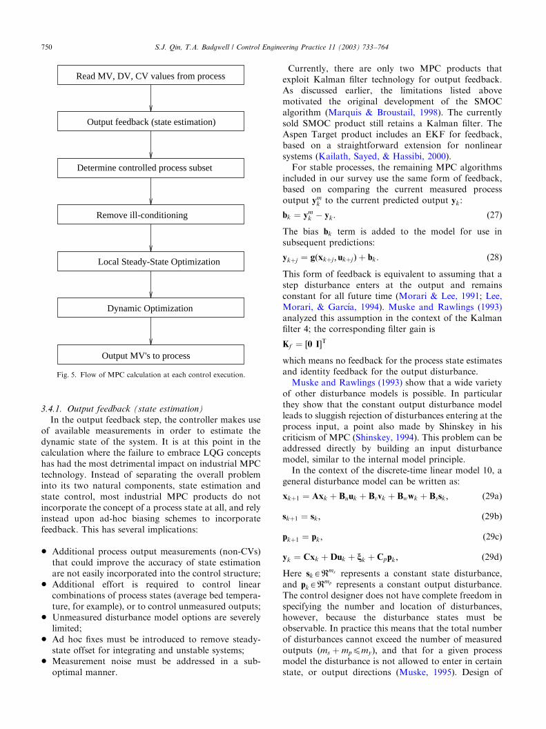
3.4.1. Output feedback (state estimation)

In the output feedback step, the controller makes useof available measurements in order to estimate thedynamic state of the system. It is at this point in thecalculation where the failure to embrace LQG conceptshas had the most detrimental impact on industrial MPCtechnology. Instead of separating the overall probleminto its two natural components, state estimation andstate control, most industrial MPC products do notincorporate the concept of a process state at all, and relyinstead upon ad-hoc biasing schemes to incorporatefeedback. This has several implications:

* Additional process output measurements (non-CVs)that could improve the accuracy of state estimationare not easily incorporated into the control structure;

* Additional effort is required to control linearcombinations of process states (average bed tempera-ture, for example), or to control unmeasured outputs;

* Unmeasured disturbance model options are severelylimited;

* Ad hoc fixes must be introduced to remove steady-state offset for integrating and unstable systems;

* Measurement noise must be addressed in a sub-optimal manner.

Currently, there are only two MPC products thatexploit Kalman filter technology for output feedback.As discussed earlier, the limitations listed abovemotivated the original development of the SMOCalgorithm (Marquis & Broustail, 1998). The currentlysold SMOC product still retains a Kalman filter. TheAspen Target product includes an EKF for feedback,based on a straightforward extension for nonlinearsystems (Kailath, Sayed, & Hassibi, 2000).For stable processes, the remaining MPC algorithms

included in our survey use the same form of feedback,based on comparing the current measured processoutput ym

k to the current predicted output yk:

bk ¼ ymk � yk: ð27Þ

The bias bk term is added to the model for use insubsequent predictions:

ykþj ¼ gðxkþj ; ukþjÞ þ bk: ð28Þ

This form of feedback is equivalent to assuming that astep disturbance enters at the output and remainsconstant for all future time (Morari & Lee, 1991; Lee,Morari, & Garc!ıa, 1994). Muske and Rawlings (1993)analyzed this assumption in the context of the Kalmanfilter 4; the corresponding filter gain is

Kf ¼ ½0 IT

which means no feedback for the process state estimatesand identity feedback for the output disturbance.Muske and Rawlings (1993) show that a wide variety

of other disturbance models is possible. In particularthey show that the constant output disturbance modelleads to sluggish rejection of disturbances entering at theprocess input, a point also made by Shinskey in hiscriticism of MPC (Shinskey, 1994). This problem can beaddressed directly by building an input disturbancemodel, similar to the internal model principle.In the context of the discrete-time linear model 10, a

general disturbance model can be written as:

xkþ1 ¼ Axk þ Buuk þ Bvvk þ Bwwk þ Bssk; ð29aÞ

skþ1 ¼ sk; ð29bÞ

pkþ1 ¼ pk; ð29cÞ

yk ¼ Cxk þDuk þ nk þ Cppk; ð29dÞ

Here skARms represents a constant state disturbance,and pkARmp represents a constant output disturbance.The control designer does not have complete freedom inspecifying the number and location of disturbances,however, because the disturbance states must beobservable. In practice this means that the total numberof disturbances cannot exceed the number of measuredoutputs ðms þ mppmyÞ; and that for a given processmodel the disturbance is not allowed to enter in certainstate, or output directions (Muske, 1995). Design of

Read MV, DV, CV values from process

Output feedback (state estimation)

Determine controlled process subset

Remove ill-conditioning

Dynamic Optimization

Local Steady-State Optimization

Output MV's to process

Fig. 5. Flow of MPC calculation at each control execution.


sensible disturbance models for MPC applications is aripe area for future academic research, especially fornonlinear systems.For stable processes, the constant output disturbance

model provides integral action to the controller,effectively removing steady-state offset due to distur-bances and model mismatch (Rawlings et al., 1994). Forintegrating and unstable processes, however, the con-stant output disturbance model fails because theestimator contains the unstable poles of the process(Muske & Rawlings, 1993). This can be addressed easilythrough the use of input or state disturbance models,but most industrial MPC are forced to address the issueusing ad hoc fixes, since they do not incorporate aKalman filter. The approach used in the DMC-plusproduct is typical, where it is assumed that a constantintegrating disturbance has entered the process, and arotation factor is used to describe the fraction ofprediction error due to the constant integrating dis-turbance, relative to the constant output disturbance.For a specific output variable that is an integratingmode, the corresponding disturbance model can berepresented as:

xkþ1 ¼ xk þ buuk þ bvvk þ bwwk þ apk; ð30aÞ

pkþ1 ¼ pk; ð30bÞ

yk ¼ cxk þ duk þ xk þ pk; ð30cÞ

where a is the rotation factor. In this case it can beshown that the disturbance pk is observable only if therotation factor a is nonzero. While this scheme providesoffset-free control for integrating systems, choice of anappropriate rotation factor is difficult in practice, andcontrol of noisy integrating systems is often poor.The MPC products include features to address a

variety of feedback scenarios encountered in applica-tions. In some cases the CV measurement may not beavailable at each control execution; this may happen, forexample, when the CV measurement is provided by ananalyzer. In this case a typical solution is to skip the biasupdate for the affected CV for a number of controlintervals. A counter is provided to disable control of theCV if too many executions go by without feedback.

3.4.2. Determining the controlled sub-process

After the process state has been estimated, thecontroller must determine which MVs can be manipu-lated and which CVs should be controlled. In general, ifthe measurement status for a CV is good, and theoperator has enabled control of the CV, then it shouldbe controlled. An MV must meet the same criteria to beused for control; in addition, however, the lower levelcontrol functions must also be available for manipula-tion. If the lower level controller is saturated high orlow, one can add a temporary hard MV constraint to the

problem to prevent moving the MV in the wrongdirection. If the lower level control function is disabled,the MV cannot be used for control. In this case it shouldbe treated as a DV. From these decisions a controlledsubprocess is defined at each control execution. Ingeneral the shape of the subprocess changes in real-timeas illustrated in Fig. 3.In applications, it is typical to include the low level

control outputs (e.g., valve positions) in the MPCcontrol formulation as additional CVs. These CVs arethen forced to stay within high and low saturation limitsby treating them as range or zone control variables. Thisserves to keep the lower level controllers away fromvalve constraints that would otherwise compromise theirperformance.In most MPC products, sensor faults are limited to

complete failure that goes beyond pre-specified controllimits. Sensor faults such as significant bias and driftingthat are within normal limits are generally not detectedor identified in these products.The DMC-plus, Connoisseur, and RMPCT algorithms

distinguish between a critical CV failure and a non-

critical CV failure. If a noncritical CV fails, the RMPCTand DMC-plus algorithms continue control action bysetting the failed CV measurement to the model predictedvalue, which means there is no feedback for the failedCV. If the noncritical CV fails for a specified period oftime, RMPCT drops this CV from the control objectivefunction. If a critical CV fails, the DMC-plus andRMPCT controllers turn-off immediately.

3.4.3. Removal of ill-conditioning

At any particular control execution, the processencountered by the controller may require excessiveinput movement in order to control the outputsindependently. This problem may arise, for example, iftwo controlled outputs respond in an almost identicalway to the available inputs. Consider how difficult itwould be to independently control adjacent traytemperatures in a distillation column, or to controlboth regenerator and cyclone temperature in an FCCU.It is important to note that this is a feature of the process

to be controlled; any algorithm which attempts tocontrol an ill-conditioned process must address thisproblem. A high condition number in the process gainmatrix means that small changes in controller error willlead to large MV moves.Although the conditioning of the full control problem

will almost certainly be checked at the design phase, it isnearly impossible to check all possible sub-processeswhich may be encountered during future operation. It istherefore important to examine the condition number ofthe controlled sub-process at each control execution andto remove ill-conditioning in the model if necessary.Two strategies are currently used by MPC controllers to


accomplish this task; singular value thresholding, andinput move suppression.The singular value thresholding (SVT) method used

by the RMPCT controller involves decomposing theprocess model based on singular values using URVdecomposition. Singular values below a thresholdmagnitude are discarded, and a process model with alower condition number is then reassembled and usedfor control. The neglected singular values representdirections along which the process hardly moves even ifa large MV change is applied; the SVT method gives upthese directions to avoid erratic MV changes. Thismethod solves the ill-conditioning problem at theexpense of neglecting the smallest singular values. Ifthe magnitude of the neglected singular values is smallcompared to the model uncertainty, it may be better toneglect them anyway. After SVT, the collinear CVs areapproximated with the principal singular direction. Inthe case of two collinear CVs, for example, this principaldirection is a weighted average of the two CVs. Notethat the SVT approach is sensitive to output weighting.If one CV is weighted much more heavily than another,this CV will represent the principal singular direction.Controllers that use input move suppression (IMS),

such as the DMC-plus algorithm, provide an alternativestrategy for dealing with ill-conditioning. Input movesuppression factors increase the magnitude of thediagonal elements of the matrix to be inverted in theleast-squares solution, directly lowering the conditionnumber. The move suppression values can be adjustedto the point that erratic input movement is avoided forthe commonly encountered sub-processes. In the case oftwo collinear CVs, the move suppression approach givesup a little bit on moving each CV towards its target. Themove suppression solution is similar to that of the SVTsolution in the sense that it tends to minimize the normof the MV moves. In the limit of infinite movesuppression the condition number becomes one for allsub-processes. It would be useful to find a set of finitemove suppression factors which guarantee that all sub-processes have a condition number greater than adesired threshold value; the authors are not aware ofany academic work that addresses this question.

3.4.4. Local steady-state optimization

Almost all of the MPC products we surveyed performa separate local steady-state optimization at eachcontrol cycle to compute steady-state input, state, oroutput targets. This is necessary because the optimaltargets may change at any time step due to disturbancesentering the loop or operator inputs that redefine thecontrol problem. The optimization problem is typicallyformulated so as to drive steady-state inputs andoutputs as closely as possible to targets determined bythe local economic optimization (just above the MPCalgorithm in Fig. 2), without violating input and output

constraints. Constant disturbances estimated in theoutput feedback step appear explicitly in the steady-state optimization so that they can be removed. Rao andRawlings describe a representative formulation of theproblem (Rao & Rawlings, 1999). The local steady-stateoptimization uses a steady-state model which may comefrom linearizing a comprehensive nonlinear model ateach control execution or may simply be the steady-stateversion of the dynamic model used in the dynamicoptimization.The Connoisseur controller uses a Linear Program

(LP) to do the local steady-state optimization. Thedistinguishing feature of an LP solution is that theoptimal steady-state targets will lie at the vertex ofthe constraint boundary. If the constraint boundarychanges frequently due to model mismatch or noise, theoptimal steady-state solution may bounce aroundunnecessarily, leading to poor overall control perfor-mance. Typical solutions to this problem include heavilyfiltering the output signals and detuning the optimizerby adding a term that minimizes movement of thesolution. These solutions slow down the movement ofthe steady-state target but also hamper rejection ofprocess disturbances. An alternative solution based ondirect incorporation of model uncertainty has beenproposed, but has not yet been implemented commer-cially (Kassmann, Badgwell, & Hawkins, 2000).The RMPCT, PFC, Aspen Target, MVC, and process

perfecter algorithms use Quadratic Programs (QP) forthe steady-state target calculation. The QP solution doesnot necessarily lie at the constraint boundary, so theoptimal steady-state targets tend not to bounce aroundas much as for an LP solution.The DMC-plus algorithm solves the local steady-state

optimization problem using a sequence of LPs and/orQPs. CVs are ranked by priority such that controlperformance of a given CV will never be sacrificed inorder to improve performance of a lower priority CV.The prediction error can be spread across a set of CVsby grouping them together at the same priority level.The calculation proceeds by optimizing the highestpriority CVs first, subject to hard and soft outputconstraints on the same CVs and all input hardconstraints. Subsequent optimizations preserve thefuture trajectory of high priority CVs through the useof equality constraints. Likewise inputs can be ranked inpriority order so that inputs are moved sequentiallytowards their optimal values when extra degrees offreedom permit.All of the products we surveyed enforce hard input

constraints in the steady-state optimization. One canalways find steady-state targets that are feasible withrespect to the input constraints, provided they aredefined in a sensible way. The same is not true, however,for output constraints. This is because if a largedisturbance enters the process, it may not be possible,


oscar

Realce

given the available input space, to completelyremove the disturbance at steady-state. For this reason,the DMC-plus, SMOC, MVC, and Process Perfecterproducts provide for soft output constraints in thesteady-state optimization. These allow for some viola-tion of an output constraint, but the magnitude of theviolation is minimized in the objective function. Theremaining products may be subject to steady-stateinfeasibility problems unless other precautions aretaken.Similar infeasibility problems may arise due to failure

to zero out integrating modes of the process at steadystate. The DMC-plus algorithm, for example, includesan explicit constraint that forces integrating (ramp) CVvariables to line out at steady state. If this constraint isviolated, due perhaps to a large disturbance entering theloop, the DMC-plus product will shut off with awarning message. Other products most likely addressthis issue in a similar way. An alternative solution is topenalize the violation using a soft constraint, so that thecontroller will try its best to line out the integrating CVsat steady state without shutting off. If the disturbancediminishes, or the operator provides more room with theinput constraints, it is possible that the next steady-statecalculation will be feasible.The NOVA-NLC controller does not perform a

separate steady-state optimization; the steady-state anddynamic optimizations are performed simultaneously.This may improve controller performance as longas the steady-state and dynamic objectives do notconflict. For example, with separate objectivesit is possible that a steady-state target may be computedthat cannot be achieved, due to constraints that appearonly in the dynamic optimization. Combining theobjectives leads to a more complex numerical problem,however.

3.4.5. Dynamic optimization

At the dynamic optimization level, an MPC controllermust compute a set of MV adjustments that will drivethe process to the desired steady-state operatingpoint without violating constraints. All of theMPC products we surveyed can be described (approxi-mately) as minimizing the following dynamic objectivefunction:

JðuM Þ ¼XP

j¼1

fjjeykþj jj

qQj

þ jjsj jjqTg

þXM�1

j¼0

fjjeukþj jj

qRjþ jjDukþj jj

qSjg ð31aÞ

subject to a model constraint:

xkþj ¼ fðxkþj�1; ukþj�1Þ 8j ¼ 1;P;

ykþj ¼ gðxkþj ; ukþjÞ 8j ¼ 1;Pð31bÞ

and subject to inequality constraints:

%y� sjpykþjp%yþ sj 8j ¼ 1;P;

sjX0 8j ¼ 1;P;

%upukþjp%u 8j ¼ 0;M � 1;

D%upDukþjpD%u 8j ¼ 0;M � 1:

ð31cÞ

The objective function in Eq. (31a) involves fourconflicting contributions. Future output behavior iscontrolled by penalizing deviations from the desiredoutput trajectory yr

kþj ; defined as eykþj ykþj � yr

kþj ;over a prediction horizon of length P: Output constraintviolations are penalized by minimizing the size of outputconstraint slack variables sj : Future input deviationsfrom the desired steady-state input us are controlledusing input penalties defined as eu

kþj ukþj � us; over acontrol horizon of length M: Rapid input changes arepenalized with a separate term involving the movesDukþj : The size of the deviations is measured by a vectornorm, usually either an L1 or L2 norm ðq ¼ 1; 2Þ: Therelative importance of the objective function contribu-tions is controlled by setting the time dependent weightmatrices Qj ; Tj ; Sj ; and Rj ; these are chosen to bepositive semi-definite. The solution is a set of M inputadjustments:

uM ¼ ðuk; ukþ1;y; ukþM�1Þ: ð32Þ

Most of the MPC controllers use a quadratic objectivefunction similar to 31a ðq ¼ 2Þ for the dynamicoptimization. For this case the dynamic optimizationtakes the form of a QP, and can be solved reliably usingstandard software. However, for very large problems, orvery fast processes, there may not be sufficient timeavailable to solve a QP. For these reasons the DMC-plusand PFC algorithms use fast sub-optimal algorithms togenerate approximate solutions to the dynamic optimi-zation. In the DMC-plus algorithm, when an input ispredicted to violate a maximum or minimum limit it isset equal to the limit and the calculation is repeated withthe MV removed. The PFC algorithm performs thecalculation without constraints and then clips the inputvalues if they exceed hard constraints. Both of thesetechniques will prevent violation of hard input con-straints but will, in general, involve a loss of perfor-mance that is difficult to predict. Typically the resultingperformance is acceptable, but the solutions do notsatisfy the Karush–Kuhn–Tucker necessary conditionsfor optimality.The DMC-plus and SMOC algorithms penalize only

the last input deviation in order to drive the systemtowards the optimal steady state:

Rj ¼ 0 8joM � 1;

RM�1b0: ð33Þ

If the final input weight is large enough and the processis stable, this is approximately equivalent to having a


terminal state constraint. If the dynamic solution at theend of the horizon is significantly different from thesteady-state targets, which means the terminal states arenot effectively constrained, the DMC-plus controllerwill automatically turn off. This setting effectivelyprovides nominal stability for DMC-plus controller.The final input weights are also applicable to integratingprocesses where the derivative of the integrator is drivento zero.The RMPCT, HIECON, PFC, and SMOC algo-

rithms do not penalize input moves directly (Sj=0). TheHIECON and PFC algorithms use a predefined outputreference trajectory to avoid aggressive MV moves. TheRMPCT controller defines a funnel, which will bedescribed later in the paper, and finds the optimaltrajectory and optimal MV moves by minimizing:

ðuM ; yrÞ ¼ arg minXP

j¼1

jjykþj � yrkþj jj

2Q

þ jjukþM�1 � usjj2R ð34Þ

subject to the funnel constraints. The relative priority ofthe two terms is set by the two weighting matrices. In thecase that the first term is completely satisfied, which istypical due to the funnel formulation, the CV error willvanish and the minimization is in fact performed on thesecond term only. In this case the results will be similarto having two separate objectives on CVs and MVs. Inthe case of an infinite number of solutions, which is alsotypical due to ‘‘relaxing’’ the trajectory, a minimumnorm solution to the MVs is obtained due to the use ofsingular value thresholding.Using a single objective function in the dynamic

optimization means that trade-offs between the fourcontributions must be resolved using the relative weightmatrices Qj ; Tj ; Sj ; and Rj : The HIECON algorithmresolves conflicting dynamic control objectives bysolving separate CV and MV optimization problems.The decision is made, a priori, that CV errors are moreimportant than MV errors. A quadratic output optimi-zation problem is solved first, similar to 31 but includingonly the e

ykþj terms. For the thin and square plant cases

this will provide a unique solution and the calculationterminates. For the fat plant case there are remainingdegrees of freedom that can be used to optimize theinput settings. For this case the controller solves aseparate quadratic input optimization problem, similarto 31 but including only the eu

kþj terms. The inputoptimization includes a set of equality constraints thatpreserve the future output trajectories found in theoutput optimization. This eliminates the need to setweights to determine the trade-off between output andinput errors, at the cost of additional computation.The PFC controller includes only the process input

and output terms in the dynamic objective, and usesconstant weight matrices ðQj ¼ Q; Tj ¼ 0; Rj ¼ R; Sj ¼

0; q ¼ 2). The Aspen Target and MVC products includeall four terms with constant weights (Qj ¼ Q; Tj ¼ T;Rj ¼ R; Sj ¼ S; q ¼ 2). The NOVA-NLC product addsto this the option of one norms (Qj ¼ Q; Tj ¼ T; Rj ¼R; Sj ¼ S; q ¼ 1; 2).Instead of using a reference trajectory, the Process

Perfecter product (Tj ¼ T; Rj ¼ 0; Sj ¼ 0; q ¼ 2) uses adynamic objective with trajectory weighting that makesQj gradually increase over the horizon P: With this typeof weighting, control errors at the beginning of thehorizon are less important than those towards the end ofthe horizon, thus allowing a smoother control action.

3.4.6. Constraint formulations

There are three types of constraints commonly used inindustrial MPC technology; hard, soft, and setpointapproximation. These are illustrated in Fig. 6. Hardconstraints, shown in the top of Fig. 6, are those whichshould never be violated. Soft constraints, shown in themiddle of Fig. 6 are those for which some violation maybe allowed; the violation is typically minimized using aquadratic penalty in the objective function.

past futureHard Constraint

Setpoint approximation of Soft Constraint

past futureSoft Constraint

quadratic penalty

past future

quadratic penalty

Fig. 6. The three basic types of constraint; hard, soft and setpoint

approximation. Hard constraints (top) should not be violated in the

future. Soft constraints (middle) may be violated in the future, but the

violation is penalized in the objective function. Setpoint approximation

of constraint (bottom) penalizes deviations above and below the

constraint. Shades areas show violations penalized in the dynamic

optimization. Adapted from Froisy (1994).


Another way to handle soft constraints is to use asetpoint approximation, as illustrated at the bottom ofFig. 6. Setpoints are defined for each soft constraint,resulting in objective function penalties on both sides ofthe constraint. The output weight is adjusted dynami-cally, however, so that the weight becomes significantonly when the CV comes close to the constraint. When aviolation is predicted the weight is increased to a largevalue so that the control can bring the CV back to itsconstraint limit. As soon as the CV is within theconstraint limit, the steady-state target is used as thesetpoint instead.All of the MPC algorithms allow hard MV maximum,

minimum, and rate of change constraints to be defined.These are generally defined so as to keep the lower levelMV controllers in a controllable range, and to preventviolent movement of the MVs at any single controlexecution. The PFC algorithm also accommo-dates maximum and minimum MV acceleration con-straints which are useful in mechanical servo controlapplications.With the exception of the DMC-plus algorithm, all of

the MPC products enforce soft output constraints in thedynamic optimization. Hard output constraints areprovided as options in the PFC, HIECON, andNOVA-NLC algorithms, but these must be used care-fully, because enforcement of hard output constraintscan lead to closed-loop instability for nonminimumphase processes (Zafiriou, 1990; Muske & Rawlings,1993). Hard output constraints can also cause feasibilityproblems, especially if a large disturbance enters theprocess. In the PFC and HIECON algorithms, hardoutput constraints are ranked in order of priority so thatlow priority constraints can be dropped when theproblem becomes infeasible. The Connoisseur algorithmprovides constraint optimization to match the numberof active constraints with the number of degrees offreedom available to the controller, i.e., the number ofunconstrained MVs.

3.4.7. Output and input trajectories

Industrial MPC controllers use four basic options tospecify future CV behavior; a setpoint, zone, referencetrajectory or funnel. These are illustrated in Fig. 7. Theshaded areas correspond to the e

ykþj and eu

kþj terms in31a. All of the controllers provide the option to drive theCVs to a fixed setpoint, with deviations on both sidespenalized in the objective function. In practice this typeof specification is very aggressive and may lead to verylarge input adjustments, unless the controller is detunedin some fashion. This is particularly important when theinternal model differs significantly from the process.Several of the MPC algorithms use move suppressionfactors for this purpose.All of the controllers also provide a CV zone control

option, designed to keep the CV within a zone defined

by upper and lower boundaries. One way to implementzone control is to define upper and lower softconstraints. Other implementations are possible, how-ever. The DMC-plus algorithm, for example, uses thesetpoint approximation of soft constraints to implementthe upper and lower zone boundaries.The HIECON, PFC, SMOC, Aspen Target, MVC,

and NOVA-NLC algorithms provide an option tospecify a desired future path for each CV called areference trajectory. A first or second order curve isdrawn from the current CV value to the setpoint, withthe speed of the response determined by one or moretrajectory time constants. Future CV deviations fromthe reference trajectory are penalized. In the limit of zerotime constants the reference trajectory reverts back to apure setpoint; for this case, however, the controllerwould be sensitive to model mismatch unless some otherstrategy such as move suppression is also being used. Adrawback of the reference trajectory formulation is that

past future

past future

quadratic penalty

past future

quadratic penalty

past future

quadratic penalty

Setpoint

Zone

Reference Trajectory

Funnel

quadratic penalty

Fig. 7. Four options for specifying future CV behavior; setpoint, zone,

reference trajectory and funnel. Shaded areas show violations

penalized in the dynamic optimization.


it penalizes the output when it happens to drift tooquickly towards the setpoint, as might happen inresponse to an unmeasured disturbance. If the CVmoves too quickly due to model mismatch, however, thereference trajectory is beneficial in that it will slow downthe CV and minimize overshoot. The reference trajec-tory can be interpreted mathematically as a filter in thefeedback path, similar to the robustness filter recom-mended by IMC theory (Morari & Zafiriou, 1989). Ingeneral, as the reference trajectory time constantsincrease, the controller is able to tolerate larger modelmismatch.The NOVA-NLC reference trajectory is slightly more

general in that it allows separate specification of upperand lower trajectories with different dynamics andsetpoints. In the controller objective, only deviationsabove the upper trajectory and deviations below thelower trajectory are penalized. This provides additionalfreedom during the transient that the controller canutilize for other tasks.The RMPCT algorithm attempts to keep each CV

within a user defined zone, with setpoints defined bysetting the maximum and minimum zone limits equal toeach other. When the CV goes outside the zone, theRMPCT algorithm defines a CV funnel, shown at thebottom of Fig. 7, to bring the CV back within its range.The slope of the funnel is determined by a user definedperformance ratio, defined as the desired time to returnto the zone divided by the open-loop response time. Aweighted average open-loop response time is used formultivariable systems.The SMOC algorithm uses a variation of funnel when

a zone CV falls out of its range. In this case a zone withreference trajectory bounds is defined to drive the CVback into the control zone.The NOVA-NLC upper and lower trajectories,

RMPCT funnel, and SMOC reference trajectory boundsare advantageous in that if a disturbance causes thepredicted future CV to reach the setpoint more quickly

than a reference trajectory allows, the controller willtake no action. This effectively frees up degrees offreedom for the controller to achieve other objectives. Inthe same situation, other controllers would move theinputs to bring the CV back onto the defined trajectory.This is illustrated in Fig. 8 for the case of the RMPCTfunnel.All of the MPC algorithms surveyed here provide MV

setpoints to drive the inputs towards their optimalvalues when there are sufficient degrees of freedom.

3.4.8. Output horizon and input parameterization

Industrial MPC controllers generally evaluate futureCV behavior over a finite set of future time intervalscalled the prediction horizon. This is illustrated at the topof Fig. 9. The finite output horizon formulation is used

CV

SP

A

B

DV

Funnel

(b)CV

SP

A

B

(a)

DV

Fig. 8. MPC based on a funnel allows a CV to move back to the setpoint faster than a trajectory would require if a pulse disturbance releases. A

trajectory based MPC would try to move away from the setpoint to follow the trajectory.

Coincidence Points

past future

past future

prediction horizon P

Finite Horizon

Fig. 9. Output horizon options. Finite horizon (top) includes P future

points. A subset of the prediction horizon, called the coincidence

points (bottom) may also be used. Shaded areas show violations

penalized in the dynamic optimization.


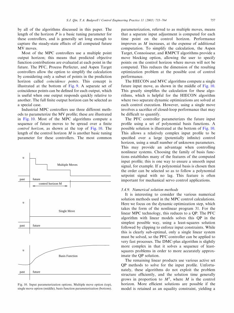
by all of the algorithms discussed in this paper. Thelength of the horizon P is a basic tuning parameter forthese controllers, and is generally set long enough tocapture the steady-state effects of all computed futureMV moves.Most of the MPC controllers use a multiple point

output horizon; this means that predicted objectivefunction contributions are evaluated at each point in thefuture. The PFC, Process Perfecter, and Aspen Targetcontrollers allow the option to simplify the calculationby considering only a subset of points in the predictionhorizon called coincidence points. This concept isillustrated at the bottom of Fig. 9. A separate set ofcoincidence points can be defined for each output, whichis useful when one output responds quickly relative toanother. The full finite output horizon can be selected asa special case.Industrial MPC controllers use three different meth-

ods to parameterize the MV profile; these are illustratedin Fig. 10. Most of the MPC algorithms compute asequence of future moves to be spread over a finitecontrol horizon, as shown at the top of Fig. 10. Thelength of the control horizon M is another basic tuningparameter for these controllers. The most common

parameterization, referred to as multiple moves, meansthat a separate input adjustment is computed for eachtime point on the control horizon. Performanceimproves as M increases, at the expense of additionalcomputation. To simplify the calculation, the AspenTarget, Connoisseur, and RMPCT algorithms provide amove blocking option, allowing the user to specifypoints on the control horizon where moves will not becomputed. This reduces the dimension of the resultingoptimization problem at the possible cost of controlperformance.The HIECON and MVC algorithms compute a single

future input move, as shown in the middle of Fig. 10.This greatly simplifies the calculation for these algo-rithms, which is helpful for the HIECON algorithmwhere two separate dynamic optimizations are solved ateach control execution. However, using a single moveinvolves a sacrifice of closed-loop performance that maybe difficult to quantify.The PFC controller parameterizes the future input

profile using a set of polynomial basis functions. Apossible solution is illustrated at the bottom of Fig. 10.This allows a relatively complex input profile to bespecified over a large (potentially infinite) controlhorizon, using a small number of unknown parameters.This may provide an advantage when controllingnonlinear systems. Choosing the family of basis func-tions establishes many of the features of the computedinput profile; this is one way to ensure a smooth inputsignal, for example. If a polynomial basis is chosen thenthe order can be selected so as to follow a polynomialsetpoint signal with no lag. This feature is oftenimportant for mechanical servo control applications.

3.4.9. Numerical solution methods

It is interesting to consider the various numericalsolution methods used in the MPC control calculations.Here we focus on the dynamic optimization step, whichtakes the form of the nonlinear program 31. For thelinear MPC technology, this reduces to a QP. The PFCalgorithm with linear models solves this QP in thesimplest possible way, using a least-squares solutionfollowed by clipping to enforce input constraints. Whilethis is clearly sub-optimal, only a single linear systemmust be solved, so the PFC controller can be applied tovery fast processes. The DMC-plus algorithm is slightlymore complex in that it solves a sequence of least-squares problems in order to more accurately approx-imate the QP solution.The remaining linear products use various active set

QP methods to solve for the input profile. Unfortu-nately, these algorithms do not exploit the problemstructure efficiently, and the solution time generallygrows in proportion to M3; where M is the controlhorizon. More efficient solutions are possible if themodel is retained as an equality constraint, yielding a

past future

u

control horizon M

Multiple Moves

past future

past future

Single Move

Basis Function

u

u

Fig. 10. Input parameterization options. Multiple move option (top),

single move option (middle), basis function parameterization (bottom).


solution time that grows linearly in proportion to M:Rao, Wright, and Rawlings describe one such methodbased on interior point techniques (Rao, Wright, &Rawlings, 1998).The nonlinear MPC products must of course use

more powerful solution techniques; these are usuallybased upon a sequence of iterations in which a linearizedversion of the problem is solved. The Aspen Targetproduct uses a multi-step Newton-type algorithmdeveloped by De Oliveira and Biegler (1995, 1994),named QPKWIK, which has the advantage thatintermediate solutions, although not optimal, areguaranteed feasible. This permits early termination ofthe optimization algorithm if necessary which guaran-tees a feasible solution. Aspen Target uses the sameQPKWIK engine for local steady-state optimization andthe dynamic MV calculation.The MVC and process perfecter products use a

generalized reduced gradient code called GRG2 devel-oped by Lasdon and Warren (1986). The NOVA-NLCproduct uses the NOVA optimization package, aproprietary mixed complementarity nonlinear program-ming code developed by DOT Products.The PFC controller, when used with a nonlinear

model, performs an unconstrained optimization using anonlinear least-squares algorithm. The solution can becomputed very rapidly, allowing the controller to beused for short sample time applications such as missiletracking. Some performance loss may be expected,however, since input constraints are enforced byclipping.

4. Applications summary

Tables 6 and 7 summarize the reported applications oflinear and nonlinear MPC technology through 1999. Itis important to note that the vendors were free to definewhat constitutes an application; for this reason one mustbe careful when drawing conclusions from these data.

For example, in some cases a single application may bedefined as a large MPC controller that encompasses anentire chemical plant. In other cases, such as anautomobile engine control, the vendor may report asingle application even when several thousand copies ofthe completed controller are sold. Note also that this is acount of MPC applications performed by the vendorsthemselves; this does not include a significant number ofin-house applications performed by licensees of vendortechnology, such as ExxonMobil and DuPont. Nor doesit include any consideration of MPC technologydeveloped completely in-house by operating companiessuch as Eastman Chemical.More than 4600 total MPC applications are reported

in Tables 6 and 7, over twice the number in our previoussurvey from 5 years earlier (Qin & Badgwell, 1997). It istherefore safe to conclude that overall usage of MPCtechnology is still growing rapidly. All of the vendorsreport a significant number of applications in progressso it is likely that this number will continue to increasein the coming years. It should be noted that the size ofthese applications ranges from a single variable toseveral hundreds of variables. Therefore, one should notuse the number of applications as an indication ofmarket share.Tables 6 and 7 show that MPC technology can now

be found in a wide variety of application areas. Thelargest single block of applications is in refining, whichamounts to 67% of all classified applications. This isalso one of the original application areas where MPCtechnology has a solid track record of success. Asignificant number of applications can also be found inpetrochemicals and chemicals, although it has takenlonger for MPC technology to break into these areas.Significant growth areas include the chemicals, pulp andpaper, food processing, aerospace and automotiveindustries.Table 6 shows that AspenTech and Honeywell Hi-

Spec are highly focused in refining and petrochemicals,with a handful of applications in other areas. Adersa

Table 7

Summary of nonlinear MPC applications by areas (estimates based on vendor survey; estimates do not include applications by companies who have

licensed vendor technology)

Area Adersa Aspen Continental DOT Pavilion Total

Technology Controls Products Technologies

Air and Gas 18 18

Chemicals 2 15 5 22

Food Processing 9 9

Polymers 1 5 15 21

Pulp & Paper 1 1

Refining 13 13

Utilities 5 2 7

Unclassified 1 1 2

Total 3 6 36 5 43 93


and Invensys apparently have a broader range ofexperience with applications in the food processing,mining/metallurgy, aerospace and automotive areas,among others. The applications reported by Adersainclude a number of embedded PFC applications, so it isdifficult to report their number or distribution. Whileonly a total number was reported by SGS, this includesa number of in-house SMOC applications by Shell, sothe distribution is likely to be shifted towards refiningand petrochemical applications.The bottom of Table 6 lists the largest linear MPC

applications to date by each vendor, in the form of(outputs)�(inputs). The numbers show a difference inphilosophy that is a matter of some controversy.AspenTech prefers to solve a large control problemwith a single controller application whenever possible;they report an olefins application with 603 outputs and283 inputs. Other vendors prefer to break the problemup into meaningful sub-processes.The nonlinear MPC applications reported in Table 7

are spread more evenly among a number of applicationareas. Areas with the largest number of reported NMPCapplications include chemicals, polymers, and air andgas processing. It has been observed that the size andscope of NMPC applications are typically much smallerthan that of linear MPC applications (Martin &Johnston, 1998). This is likely due to the computationalcomplexity of NMPC algorithms.

5. Limitations of existing technology

Many of the currently available industrial MPCalgorithms suffer from limitations inherited from theoriginal DMC and IDCOM technology. Problems withthe control technology, which have been discussed byothers (Morari & Lee, 1991; Muske & Rawlings, 1993),include:

* limited model choices;* sub-optimal feedback;* lack of nominal stability;* sub-optimal or inefficient solution of the dynamic

optimization.

Two of the linear MPC algorithms, DMC-plus andHIECON, rely on convolution models (impulse and stepresponse). This can be problematic when controlling aprocess with widely varying time constants; for this caseit is typical to sacrifice dynamic control of the fastprocess modes in order to keep the model lengthreasonable. A potentially more significant problem withthe impulse and step response models is that they arelimited to strictly stable processes. While it is certainlypossible to modify the algorithms to accommodate apure integrator, these modifications may lead to otherproblems, such as adding the derivative of a noisy

output signal into the feedback path. It is not possible,in general, to represent an unstable process using animpulse response model. All of these problems can beovercome by using an auto-regressive parametric modelform such as a state-space or ARX model.The bias update feedback technique used by industrial

MPC controllers is probably the best assumption thatcan be used for stable plants in the total absence ofdisturbance and measurement information, but betterfeedback is possible if the distribution of disturbancescan be characterized more carefully. The bias updatemethod implicitly assumes that there are no stochasticdisturbances affecting the system state, and the mea-surement is perfect. Measurement noise is typically dealtwith separately in applications using ad hoc filteringtechniques. The bias update fails for purely integratingsystems, so a number of ad hoc methods have beendeveloped by practitioners to handle this case. Thesemethods tend to work poorly in the presence ofsignificant measurement noise. Industrial practitionersneed to recognize that the Kalman filter provides a richframework to address these problems. Muske andRawlings have demonstrated how better performancecan be achieved for MPC applications by using a state-space model and an optimal state observer (Muske &Rawlings, 1993). Of course, these problems motivatedthe original development of the SMOC algorithm(Marquis & Broustail, 1998), which uses a Kalman filterfor feedback.Tuning MPC controllers for stable operation in the

presence of constraints may be difficult, even when theprocess model is perfect. Currently much effort is spenton closed-loop simulation prior to commissioning acontroller. It must be recognized, however, thatsimulating all possible combinations of active con-straints is impossible in practice. It seems far better tobuild an algorithm that is inherently stable in all suchcases; in control theory this is known as a nominally

stabilizing algorithm. Scokaert and Rawlings (1998)show how this can be done for the linear case by usinginfinite prediction and control horizons. Chen andAllg .ower present a quasi-infinite horizon method fornonlinear systems (Chen & Allgower, 1995). Researchresults for the nonlinear case are covered thoroughly byMayne et al. (2000). None of the currently availableindustrial MPC algorithms makes full use of these ideas.Sub-optimal solutions to the dynamic optimization 31

are used in several of the packages, presumably in orderto speed up the solution time. This seems difficult tojustify for the case of refining and petrochemicalapplications, where the controllers run on the order ofonce each minute. Goodwin et al. (2001) give anexample where unconstrained LQR solution with anti-windup has significant performance deterioration com-pared to an MPC solution under severe constraints.However, for high speed applications where the


controller must execute in a few milliseconds, such astracking the position of a missile, it may not be feasibleto solve a QP at every control execution. For this case agood sub-optimal solution may be the only option.None of the linear MPC products exploit the

structure of QP in the dynamic optimization. Thesingular value technique in RMPCT is one of the fewefforts in using robust numerical techniques. Byproperly exploiting the structure of the problem, itshould be possible to handle significantly larger and/orfaster processes (Rao et al., 1998).Model uncertainty is not addressed adequately by

current MPC technology. While most of the identifica-tion packages provide estimates of model uncertainty,only one vendor (Honeywell) provides a way to use thisinformation in the control design. All of the MPCalgorithms provide a way to detune the control toimprove robustness, but the trade-off between perfor-mance and robustness is generally not very clear. Untilthis connection is made, it will not be possible todetermine when a model is accurate enough for aparticular control application. There are many robustMPC results available in the academic literature, butmost focus only the dynamic optimization and will notwork for something as simple as a setpoint change.Promising results that may eventually impact MPCpractice include the robust stability conditions presentedby Vuthandam et al. for a modified QDMC algorithm(Vuthandam, Genceli, & Nikolaou, 1995); the robustMPC algorithm presented by Kothare, Balakrishnan,and Morari (1996) and the robust steady-state targetcalculation described by Kassmann, Badgwell, andHawkins (2000). More research is needed in this area.Current model identification technology suffers from

a number of limitations:

* plant test signals are typically step-like and requireclose attention of experienced engineers during thetest;

* there is no tool to determine whether the collecteddata are adequate to represent the process dynamicsfor MPC design; in practice the plant is generally overtested, increasing the implementation cost during thetest period;

* identification algorithms are mainly of the least-squares type; there are only a few that use modernsubspace identification and prediction error methods;

* statistical efficiency and consistency of identificationalgorithms are not addressed;

* there is a lack of model validation methods to verifywhether the identified model is adequate for controlor whether significant model deteriorationhas occurred after the MPC controller has beencommissioned;

* there is little practice except in Connoisseur inmultivariable closed-loop identification which would

be very useful for on-line model updating or adaptiveMPC implementation;

* there is no systematic approach for building non-linear dynamic models for NMPC. Guidelines forplant tests are needed to build a reliable nonlinearmodel. This is important because even more test datawill be required to develop an empirical nonlinearmodel than an empirical linear model.

6. Next-generation MPC technology

MPC vendors were asked to describe their vision ofnext-generation MPC technology. Their responses werecombined with our own views and the earlier analysis ofFroisy (1994) to come up with a composite view offuture MPC technology.

6.1. Basic controller formulation

Because it is so difficult to express all of the relevantcontrol objectives in a single objective function, next-generation MPC technology will utilize multiple objec-tive functions. The infinite prediction horizon hasbeneficial theoretical properties and will probablybecome a standard feature. Output and input trajectoryoptions will include setpoints, zones, trajectories andfunnels. Input parameterization using basis functionsmay become more widespread, and infinite controlhorizons with moves computed at each control intervalmay also become possible.

6.2. Adaptive MPC

A few adaptive MPC algorithms such as the GPCalgorithm introduced by Clarke et al. have beenproposed (Clarke, Mohtadi, & Tuffs, 1987) but onlytwo adaptive MPC algorithms have reached the market-place (Connoisseur from Invensys and STAR from DotProducts (Dollar, Melton, Morshedi, Glasgow, &Repsher, 1993)). This is despite the strong marketincentive for a self-tuning MPC controller. This reflectsthe difficulty of doing adaptive control in the real world.Barring a theoretical breakthrough, this situation is notlikely to change in the near future.On the other hand, adaptive and on-demand tuning

PID controllers have been very successful in themarketplace. This suggests that adaptive MPC con-trollers may emerge for SISO loops as adaptive PIDtechnology is generalized to handle more difficultdynamics.

6.3. Robust MPC

With one exception (Honeywell), industrial MPCcontrollers rely solely on brute-force simulation to


evaluate the effects of model mismatch. Robust stabilityguarantees would significantly reduce the time requiredto tune and test industrial MPC algorithms. It is likelythat recent robust research results (Kassmann et al.,2000; Kothare et al., 1996; Scokaert & Mayne, 1998) willeventually make their way into MPC products. Robuststability guarantees will then be combined with un-certainty estimates from identification software togreatly simplify design and tuning of MPC controllers.

6.4. Nonlinear MPC

Next-generation MPC technology will allow non-linear models to be developed by seamlessly combiningprocess knowledge with operating data. A continuous-time fundamental model will be defined from a graphicalrepresentation of the plant. Process test signals will bedesigned automatically so as to explore importantregions of the operating space where the model isinadequate for control. Closed-loop process tests will beconducted using PRBS signals, with minimal on-sitetime requirements. Owing to the difficulty in data basedmodeling of nonlinear processes, first principles modelsand other alternative modeling methods (Foss, Loh-mann, & Marquardt, 1998) will become necessary inpractice.

7. Discussion and conclusions

MPC technology has progressed steadily since the firstIDCOM and DMC applications over 25 years ago. Oursurvey data show that the number of MPC applicationshas approximately doubled in 4 years from 1995 to1999. MPC applications show a solid foundation inrefining and petrochemicals, and significant penetrationinto a wide range of application areas from chemicals tofood processing. The MPC technology landscape haschanged dramatically in recent years, making it difficultfor us to keep track of the swift progress in academicresearch and industrial applications. Major recentdevelopments include:

* Technological changes due to the development ofnew algorithms by academia and industry, computerhardware and software advances, and the breadth ofindustrial applications.

* Organizational changes due to acquisitions andmergers, such as the acquisition by Aspen Technol-ogy of DMCC, Setpoint, Treiber Controls, andNeuralware.

* Integration of MPC technology into DistributedControl System (DCS) platforms, illustrated by theacquisition of Predictive Control Ltd. by Invensys,the parent company of Foxboro.

* Increased applications by end-users who license MPCsoftware from vendors.

Current generation linear MPC technology offerssignificant new capabilities, but several unnecessarylimitations still remain. Some products do not allowthe use of parametric models. Feedback options areseverely limited, often leading to poor control ofintegrating systems and slow rejection of unmeasureddisturbances. The algorithms are not nominally stabiliz-ing, so that tuning choices must be tested extensivelythrough closed-loop simulation. None of the linearMPC algorithms makes use of modern numericalsolution methods, limiting the size and speed ofprocesses that they can be applied to.Applications of nonlinear MPC products will con-

tinue to grow in those areas where linear MPCtechnology has proven difficult to apply, such as controlof polymerization processes. The nonlinear MPC algo-rithms reported here differ in the simplifications used togenerate a tractable control calculation. The models areusually specified as linear dynamic subsystems withadded nonlinearity. The NOVA-NLC controller is theonly current offering that allows the use of a rigorousnonlinear model derived from first principles.An important observation is that the majority of

industrial MPC controllers use empirical dynamicmodels identified from test data. Improvements inidentification technology that result in shorter overallprocess testing times will have a large positive impact onthe bottom line for MPC technology users.Choosing an MPC technology for a given application

is a complex question involving issues not addressed inthis paper. Here, we have emphasized the technicalcapabilities of MPC technology. However, if a vendor isto be selected to design and implement an advancedcontrol system, it would be wise to weigh heavily theirexperience with the particular process in question.Research needs as perceived by industry are mostly

control engineering issues, not algorithm issues. Indus-trial practitioners do not perceive closed-loop stability,for example, to be a serious problem. Their questionsare more like: Which variables should be used forcontrol? When is a model good enough to stop theidentification plant test? How do you determine thesource of a problem when a controller is performingpoorly? When can the added expense of a nonlinearMPC controller be justified? How do you design acontrol system for an entire plant? How do you estimatethe benefits of a control system? Answering thesequestions will provide control practitioners and theore-ticians with plenty of work in the foreseeable future.Just as academicians do not agree on which control

algorithms are best, industrial practitioners also havevery different views on the future trends of MPC. Just asPID controllers have many different implementations


(series form, parallel form, etc.), MPC controllers arenot anticipated to converge to a single form in theforeseeable future. While academic research will con-tinue to develop new algorithms and prove new facts inthe MPC domain, industrial development will considerits own priorities with a healthy interaction withacademia. Although there is still plenty of room torefine or develop new MPC algorithms, pushing thetechnology to new application areas could be at leastequally important and challenging. Given the unevendistribution in the MPC applications today, it is safe toanticipate that much more development in both theoryand practice is still ahead of us.

Acknowledgements

The authors wish to thank the vendor representativeswho responded to our MPC survey for their time andeffort. We also wish to thank the following people fortheir constructive criticism of this paper: Pierre Carrette,Jim Downs, Harry Forbes, Brian Froisy, Pierre Gros-didier, John Guiver, Rob Hawkins, Dean Kassmann,Geoff Lewis, Joseph Lu, Greg Martin, Steve Piche, JimRawlings, Jaques Richalet, Andy Speziale, DouglasWhite, Robert Young, and Hong Zhao.

References

Allgower, F., Badgwell, T. A., Qin, S. J., Rawlings, J. B., & Wright,

S. J. (1999). Nonlinear predictive control and moving horizon

estimation—an introductory overview. In P. M. Frank (Ed.),

Advances in control: highlights of ECC ’99. Berlin: Springer.

Allgower, F., & Zheng, A., (Eds.). (2000). Nonlinear model predictive

control, progress in systems and control theory. Vol. 26. Basel,

Boston, Berlin: Birkhauser Verlag.

Bartusiak, R. D., & Fontaine, R. W. (1997). Feedback method for

controlling non-linear processes. US Patent 5682309.

Berkowitz, P., & Papadopoulos, M. (1995). Multivariable process

control method and apparatus. US Patent 5396416.

Berkowitz, P., Papadopoulos, M., Colwell, L., & Moran, M. (1996).

Multivariable process control method and apparatus. US Patent

5488561.

Chen, H., & Allgower, F. (1995). A quasi-infinite horizon nonlinear

model predictive control scheme with guaranteed stability. Auto-

matica, 34(10), 1205–1218.

Clarke, D. W., Mohtadi, C., & Tuffs, P. S. (1987). Generalized

predictive control—Part I. The basic algorithm. Automatica, 23(2),

137–148.

MVC 3.0 User Manual (1995). Continental Controls, Inc. Product

Literature.

Cutler, C., Morshedi, A., & Haydel, J. (1983). An industrial

perspective on advanced control. In AICHE annual meeting,

Washington, DC, October 1983.

Cutler, C. R., & Ramaker, B. L. (1979). Dynamic matrix control—a

computer control algorithm. AICHE national meeting, Houston,

TX, April 1979.

Cutler, C. R., & Ramaker, B. L. (1980). Dynamic matrix control—a

computer control algorithm. In Proceedings of the joint automatic

control conference.

Cutler, C. R., & Yocum, F. H. (1991). Experience with the DMC

inverse for identification. In Y. Arkun, W. H. Ray (Eds.), Chemical

process control—CPC IV. Fourth international conference on

chemical process control (pp. 297–317). Amsterdam: Elsevier.

Demoro, E., Axelrud, C., Johnston, D., & Martin, G. (1997). Neural

network modeling and control of polypropylene process. In Society

of plastics engineers international conference, Houston, TX.

DMC Corp. ½DMCTM (1994). Technology overview. Product literature

from DMC Corp., July 1994.

Dollar, R., Melton, L. L., Morshedi, A. M., Glasgow, D. T., &

Repsher, K. W. (1993). Consider adaptive multivariable predictive

controllers. Hydrocarbon Processing, 10, 109–112.

Downs, J. J. (2001). Linking control strategy design and model

predictive control. In Preprints: Chemical process control-6,

assessment and new directions for research (CPC VI), Tuscon,

AZ, January 2001 (pp. 411–422).

Foss, B. A., Lohmann, B., & Marquardt, W. (1998). A field study of

the industrial modeling process. Journal of Process Control, 8(5,6),

325–338.

Froisy, J. B. (1994). Model predictive control: Past, present and future.

ISA Transactions, 33, 235–243.

Froisy, J. B., & Matsko, T. (1990). IDCOM-M application to the Shell

fundamental control problem. AICHE annual meeting, November

1990.

Garc!ıa, C. E., & Morshedi, A. M. (1986). Quadratic programming

solution of dynamic matrix control (QDMC). Chemical Engineer-

ing Communications, 46, 73–87.

Garc!ıa, C. E., Prett, D. M., & Morari, M. (1989). Model predictive

control: Theory and practice—a survey. Automatica, 25(3), 335–348.

Goodwin, G. C., Graebe, S. F., & Salgado, M. E. (2001). Control

system design. Englewood Cliffs, NJ: Prentice Hall.

Grosdidier, P., Froisy, B., & Hammann, M. (1988). The IDCOM-M

controller. In T. J. McAvoy, Y. Arkun, & E. Zafiriou (Eds.),

Proceedings of the 1988 IFAC workshop on model based process

control (pp. 31–36). Oxford: Pergamon Press.

Hillestad, M., & Andersen, K. S. (1994). Model predictive control for

grade transitions of a polypropylene reactor. In Proceedings of the

4th European symposium on computer aided process engineering

(ESCAPE 4), Dublin, March 1994.

Honeywell Inc. (1995). RMPCT concepts reference. Product literature

from Honeywell, Inc., October 1995.

Kailath, T. (1980). Linear systems. Englewood Cliffs, NJ: Prentice-

Hall.

Kailath, T., Sayed, A. H., & Hassibi, B. (2000). Linear estimation.

Upper Saddle River, NJ: Prentice-Hall.

Kalman, R. E. (1960a). Contributions to the theory of optimal control.

Bulletin de la Societe Mathematique de Mexicana, 5, 102–119.

Kalman, R. E. (1960b). A new approach to linear filtering and

prediction problems. Transactions of ASME, Journal of Basic

Engineering, 87, 35–45.

Kassmann, D. E., Badgwell, T. A., & Hawkins, R. B. (2000). Robust

steady-state target calculation for model predictive control.

A.I.CH.E. Journal, 46(5), 1007–1024.

Keeler, J., Martin, G., Boe, G., Piche, S., Mathur, U., & Johnston, D.

(1996). The process perfecter: the next step in multivariable control

and optimization. Technical report, Pavilion Technologies, Inc.,

Austin, TX.

Kothare, M. V., Balakrishnan, V., & Morari, M. (1996). Robust

constrained model predictive control using linear matrix inequal-

ities. Automatica, 32, 1361–1379.

Kouvaritakis, B., & Cannon, M. (Eds.) (2001). Nonlinear predictive

control, theory and practice. London: The IEE.

Kulhavy, R., Lu, J., & Samad, T. (2001). Emerging technologies for

enterprise optimization in the process industries. In Preprints:

chemical process control-6, assessment and new directions for

research (CPC VI), Tuscon, Arizona, January 2001 (pp. 411–422).


Kwakernaak, H., & Sivan, R. (1972). Linear optimal control systems.

New York: Wiley.

Larimore, W. E. (1990). Canonical variate analysis in identification,

filtering and adaptive control. In Proceedings of the 29th conference

on decision and control (pp. 596–604).

Lasdon, L. S., & Warren, A. D. (1986). GRG2 user’s guide. Cleveland,

OH: Cleveland State University.

Lee, J. H., & Cooley, B. (1997). Recent advances in model predictive

control and other related areas. In J. C. Kantor, C. E. Garcia, B.

Carnahan (Eds.), Fifth international conference on chemical process

control, AICHE and CACHE, (pp. 201–216b).

Lee, E. B., & Markus, L. (1967). Foundations of optimal control theory.

New York: Wiley.

Lee, J. H., Morari, M., & Garc!ıa, C. E. (1994). State-space

interpretation of model predictive control. Automatica, 30(4),

707–717.

Lewis, D. G., Evans, C. L., & Sandoz, D. J. (1991). Application of

predictive control techniques to a distillation column. Journal of

Process Control, 1, 17–26.

Ljung, L. (1987). System identification: theory for the user. Englewood

Cliffs, NJ: Prentice-Hall, Inc.

Ljung, L. (1999). System identification: theory for the user. Englewood

Cliffs, NJ: Prentice-Hall, Inc.

Maciejowski, J. M. (2002). Predictive control with constraints. Engle-

wood Cliffs, NJ: Prentice Hall.

Marquis, P., & Broustail, J. P. (1998). SMOC, a bridge between state

space and model predictive controllers: Application to the

automation of a hydrotreating unit. In T. J. McAvoy, Y. Arkun,

& E. Zafiriou (Eds.), Proceedings of the 1988 IFAC workshop on

model based process control (pp. 37–43). Oxford: Pergamon Press.

Martin, G., & Boe, G., Keeler, J., Timmer, D., Havener, J. (1998).

Method and apparatus for modeling dynamic and steady-state

processes for prediction, control, and optimization. US Patent.

Martin, G., & Johnston, D. (1998). Continuous model-based

optimization. In Hydrocarbon processing’s process optimization

conference, Houston, TX.

Mayne, D. Q. (1997). Nonlinear model predictive control: An

assessment. In J. C. Kantor, C. E. Garcia, & B. Carnahan (Eds.),

Fifth international conference on chemical process control

AICHE and CACHE, (pp. 217–231).

Mayne, D. Q., Rawlings, J. B., Rao, C. V., & Scokaert, P. O. M.

(2000). Constrained model predictive control: Stability and

optimality. Automatica, 36, 789–814.

Morari, M., & Lee, J. H. (1991). Model predictive control: The good,

the bad, and the ugly. In Y. Arkun, & W. H. Ray (Eds.), Chemical

process control—CPC IV, Fourth international conference on

chemical process control (pp. 419–444). Amsterdam: Elsevier.

Morari, M., & Zafiriou, E. (1989). Robust process control. Englewood

Cliffs, NJ: Prentice-Hall.

Muske, K. R. (1995). Linear model predictive control of chemical

processes. PhD thesis, The University of Texas at Austin.

Muske, K. R., & Rawlings, J. B. (1993). Model predictive control with

linear models. A.I.CH.E Journal, 39(2), 262–287.

Ohshima, M., Ohno, H., & Hashimoto, I. (1995). Model predictive

control: Experiences in the university-industry joint projects and

statistics on MPC applications in Japan. International workshop on

predictive and receding horizon control, Korea, October 1995.

De Oliveira, N. M. C., & Biegler, L. T. (1995). An extension of

newtontype algorithms for nonlinear process control. Automatica,

31, 281–286.

De Oliveira, N. M. C., & Biegler, L. T. (1994). Constraint handling

and stability properties of model-predictive control. A.I.CH.E

Journal, 40(7), 1138–1155.

Piche, S., Sayyar-Rodsari, B., Johnson, D., & Gerules, M. (2000).

Nonlinear model predictive control using neural networks. IEEE

Control Systems Magazine 53–62.

Poe, W., & Munsif, H. (1998). Benefits of advanced process

control and economic optimization to petrochemical processes. In

Hydrocarbon processing’s process optimization conference, Houston,

TX.

Prett, D. M., & Garc!ıa, C. E. (1988). Fundamental process control.

Boston: Butterworths.

Prett, D. M., & Gillette, R. D. (1980). Optimization and constrained

multivariable control of a catalytic cracking unit. In Proceedings of

the joint automatic control conference.

Propoi, A. I. (1963). Use of linear programming methods for

synthesizing sampled-data automatic systems. Automatic Remote

Control, 24(7), 837–844.

Qin, S. J., & Badgwell, T. A. (1996). An overview of industrial model

predictive control technology. In Chemical process control—CPC

V, CACHE. Tahoe City, CA, January 1996.

Qin, S. J., & Badgwell, T. A. (1997). An overview of industrial model

predictive control technology. In J. C. Kantor, C. E. Garcia, & B.

Carnahan (Eds.), Chemical process control—V, Fifth international

conference on chemical process control CACHE and AICHE, (pp.

232–256).

Qin, S. J., & Badgwell, T. A. (1998). An overview of nonlinear model

predictive control applications. In F. Algower, & A. Zheng (Eds.),

Nonlinear model predictive control workshop—assessment and future

directions, Ascona, Switzerland.

Qin, S. J., & Badgwell, T. A. (2000). An overview of nonlinear model

predictive control applications. In J. C. Kantor, C. E. Garcia, & B.

Carnahan (Eds.), Nonlinear model predictive control. Basel:

Birkhauser.

Rao, C. V., & Rawlings, J. B. (1999). Steady states and constraints in

model predictive control. A.I.CH.E. Journal, 45(6), 1266–1278.

Rao, C. V., Wright, S. J., & Rawlings, J. B. (1998). Application of

interior-point methods to model predictive control. Journal of

Optimization Theory Application, 99, 723–757.

Rawlings, J. B. (2000). Tutorial overview of model predictive control.

IEEE Control Systems Magazine, 20, 38–52.

Rawlings, J. B., Meadows, E. S., & Muske, K. (1994). Nonlinear

model predictive control: a tutorial and survey. In Proceedings of

IFAC ADCHEM, Japan.

Rawlings, J. B., & Muske, K. R. (1993). Stability of constrained

receding horizon control. IEEE Transactions on Automatic Control,

38(10), 1512–1516.

Richalet, J. (1993). Industrial applications of model-based control.

Automatica, 29, 1251–1274.

Richalet, J., Rault, A., Testud, J. L., & Papon, J. (1976). Algorithmic

control of industrial processes. In Proceedings of the 4th IFAC

symposium on identification and system parameter estimation.

(pp. 1119–1167).

Richalet, J., Rault, A., Testud, J. L., & Papon, J. (1978). Model

predictive heuristic control: Applications to industrial processes.

Automatica, 14, 413–428.

Ricker, N. L. (1991). Model predictive control: State of the art. In Y.

Arkun, W. H. Ray (Eds.), Chemical process control—CPC IV,

Fourth international conference on chemical process control (pp.

271–296). Amsterdam: Elsevier.

Scokaert, P. O. M., & Mayne, D. Q. (1998). Min–max feedback model

predictive control for constrained linear systems. IEEE Transac-

tions on Automatic Control, 43(8), 1136–1142.

Scokaert, P. O. M., & Rawlings, J. B. (1998). Constrained linear

quadratic regulation. IEEE Transactions on Automatic Control,

43(8), 1163–1169.

Sentoni, G. B., Biegler, L. T., Guiver, J. B., & Zhao, H. (1998). State-

space nonlinear process modeling. A.I.CH.E Journal, 44(10),

2229–2239.

Setpoint Inc. (1993). SMC-IDCOM: A state-of-the-art multivariable

predictive controller. Product literature from Setpoint, Inc.,

October 1993.


Shinskey, F. G. (1994). Feedback controllers for the process industries.

New York: McGraw-Hill.

Vuthandam, P., Genceli, H., & Nikolaou, M. (1995). Performance

bounds for robust quadratic dynamic matrix control with end

condition. A.I.CH.E Journal, 41(9), 2083–2097.

Young, R. E., Bartusiak, R. B., & Fontaine, R. B. (2001). Evolution of

an industrial nonlinear model predictive controller. In Preprints:

Chemical process control—CPC VI, Tucson, Arizona (pp. 399–

410). CACHE.

Yousfi, C., & Tournier, R. (1991). Steady-state optimization inside

model predictive control In Proceedings of ACC’91, Boston, MA

(pp. 1866–1870).

Zafiriou, E. (1990). Robust model predictive control of processes with

hard constraints. Computers in Chemical Engineering, 14(4/5),

359–371.

Zhao, H., Guiver, J., Neelakantan, R., & Biegler, L. T. (1999). A

nonlinear industrial model predictive controller using integrated

PLS and neural state space model. In IFAC 14th triennial world

congress, Beijing, Peoples Republic of China.

Zhao, H., Guiver, J. P., & Sentoni, G. B. (1998). An identification

approach to nonlinear state space model for industrial multi-

variable model predictive control. In Proceedings of the 1998

American control conference, Philadelphia, Pennsylvannia (pp.

796–800).


mpc cep qin badgwell

Documents