Motion Fields for Interactive Character Animation

Yongjoon Lee1,2∗ Kevin Wampler1† Gilbert Bernstein1 Jovan Popovic1,3 Zoran Popovic1

1University of Washington 2Bungie 3Adobe Systems

Abstract

We propose a novel representation of motion data and control whichgives characters highly agile responses to user input and allows anatural handling of arbitrary external disturbances. Our represen-tation organizes samples of motion data into a high-dimensionalgeneralization of a vector field which we call a motion field. Ourrun-time motion synthesis mechanism freely flows through the mo-tion field in response to user commands. The motions we createappear natural, are highly responsive to real-time user input, andare not explicitly specified in the data.

CR Categories: I.3.7 [Computer Graphics]: Three-DimensionalGraphics and Realism—Animation

Keywords: animation, motion representation, data-driven anima-tion

1 Introduction

Human motion is a highly-varied and continuous phenomenon: itquickly adapts to different tasks, responds to external disturbances,and in general is capable of continuing locomotion from almost anyinitial state. As video games increasingly demand that charactersmove and behave in realistic ways, it is important to bring theseproperties of natural human motion into the virtual world. Unfor-tunately this is easier said than done. For instance, despite manyadvances in character animation techniques, creating highly agileand realistic interactive locomotion controllers remains a commonbut difficult task.

We propose a new motion representation for interactive characteranimation, termed a motion field which provides two key abilities:the ability for a user to control the character in real time and theability to operate in the fully-continuous configuration space of thecharacter. Although there exist techniques which allow one or theother of these abilities, it is the combination of the two which allowsfor highly agile controllers which can respond to user commands ina short amount of time.

More specifically, a motion field is a mapping which associates eachpossible configuration of a character with a set of motions describ-ing how the character is able to move from their current state. Inorder to generate an animation we select a single motion from thisset, follow it for a single frame, and repeat from the character’s re-sulting state. The motion of the character thus ‘flows’ through the

∗e-mail: yjlee@bungie.com†e-mail: wampler@cs.washington.edu

state space according to the integration process, similar to a particleflowing through a force field. However, instead of a single fixedflow, a motion field allows multiple possible motions at each frame.By using reinforcement learning to choose between these possibili-ties at runtime the direction of the flow can be altered, allowing thecharacter to respond optimally to user commands.

Because motion fields allow a range of actions at every frame, acharacter can immediately respond to new user commands ratherthan waiting for pre-determined transition points as in a motiongraph. This allows motion field-based controllers to be significantlymore agile than their graph-based counterparts. By further alteringthis flow with other external methods, such as inverse kinematics orphysical simulation, we also can directly integrate these techniquesinto the motion synthesis and control process. Furthermore, sinceour approach requires very little structure in the motion capture datathat it uses, minimal effort is needed to generate a new controller.The primary contribution of this work lies in the combining of acontinuous state representation with an optimal control framework.We find that this approach provides many advantages for characteranimation.

2 Related Work

In the past ten years, the bag-of-clips data structures such as mo-tions graphs have emerged as primary sources of realistic charactercontrollers [Lee et al. 2002; Arikan and Forsyth 2002; Kovar et al.2002]. These structures are inherently discrete with coarse transi-tioning abilities that provide great computational advantages. Un-fortunately, this discretization also obscures continuous propertiesof motion. First, it is difficult to create graphs which allow veryquick responses to changes of direction or unexpected disturbancessince a change to the motion can only happen when a new edge isreached [Treuille et al. 2007; McCann and Pollard 2007]. Second,because the motions are restricted to the clips which constitute thegraph it is difficult to couple these methods to physical simulatorsand other techniques which perturb the state away from states rep-resentable by the graph. More generally, it is very hard to use agraph-based controller when the character starts from an arbitrarystate configuration [Zordan et al. 2005].

Although a number of methods have been proposed to alleviatesome of the representational weaknesses of pure graph-based con-trollers, including parameterized motion graphs [Shin and Oh 2006;Heck and Gleicher 2007], increasing the numbers of possible tran-sitions [Arikan et al. 2005; Yin et al. 2005; Zhao and Safonova2008] and splicing rag doll dynamics in the graph structure [Zor-dan et al. 2005], the fundamental issue remains: unless the rep-resentation prescribes motion at every continuous state in a waythat is controllable in real time, the movement of characters willremain restricted. Hence, even when the method anticipates someuser inputs [McCann and Pollard 2007], the character may react tooslowly, or transition too abruptly because there is no shorter path inthe graph. Similarly, when methods anticipate some types of upper-body pushes [Yin et al. 2005; Arikan et al. 2005], the character maynot react at all to hand pulls or lower-body pushes.

Another group of methods use nonparametric models to learn thedynamics of character motion in a fully continuous space [Wanget al. 2008; Ye and Liu 2010; Chai and Hodgins 2005]. Thesetechniques are generally able to synthesize starting from any initial

state, and lend themselves well to applying physical disturbances[Ye and Liu 2010] and estimating a character’s pose from incom-plete data [Chai and Hodgins 2005]. These models are used toestimate a single ‘most likely’ motion for the character to take ateach possible state. This precludes the ability to optimally con-trol the character. The primary difference between our work andthese is that instead of building a model of the most probable sin-gle motion, we attempt to model the set of possible motions at eachcharacter state, and only select the single motion to use at runtimeby using principles from optimal control theory. This allows usto interactively control the character while enjoying the benefits ofa fully continuous state space. Our work combines the concepts ofnear-optimal character control present in graph-based methods withthose of nonparametric motion estimation techniques.

Although our controllers are kinematic, dynamic controllers havebeen extensively explored as an alternative method of characteranimation. In principle, such controllers offer the best possibilityfor highly realistic interactive character animation. However, high-fidelity physically based character animation is harder to attain be-cause physics alone does not tell us about the muscle forces neededto propel the characters. Despite a broad repertoire of demonstratedskills [Hodgins et al. 1995; Hodgins and Pollard 1997; Wooten andHodgins 2000; Faloutsos et al. 2001; Yin et al. 2007; Coros et al.2008b], nonparametric modeling of coarse-scale dynamics [Coroset al. 2009; Coros et al. 2008a], and use of motion capture [Laszloet al. 1996; Sok et al. 2007; da Silva et al. 2008; Muico et al. 2009],agile, lifelike, fully-dynamic characters remain an open challenge.

3 Motion Fields

Interactive applications such as video games require characters thatcan react quickly to user commands and unexpected disturbances,all while maintaining believability in the generated animation. Anideal approach would fully model the complete space of naturalhuman motion, describing every conceivable way that a charactercan move from a given state. Rather than confine motion to cannedmotion clips and transitions, such model would enable much greaterflexibility and agility of motion through the continuous space ofmotion.

Although it is infeasible to completely model the entire space ofnatural character motion, we can use motion capture data as a localapproximation. We propose a structure called a motion field thatfinds and uses motion capture data similar to the character’s currentmotion at any point. By consulting similar motions to determinewhich future behaviors are plausible, we ensure that our synthe-sized animation remains natural: similar, but rarely identical to themotion capture data. This frees the character from simply replay-ing the motion data, allowing it to move freely through the generalvicinity of the data. Furthermore, because there are always multi-ple motion data to consult, the character constantly has a variety ofways to make quick changes in motion.

3.1 Preliminary Definitions

Motion States We represent the states in which a character mightbe configured by the pose and the velocity of all of each of a char-acter’s joints. A pose x = (xroot, p0, p1, . . . , pn) consists of a3d root position vector xroot, a root orientation quaternion p0 andjoint orientation quaternions p1, . . . pn. The root point is locatedat the pelvis. A velocity v = (vroot, q0, q1, . . . , qn) consists of a3d root displacement vector vroot, root displacement quaternion q0,and joint displacement quaternions q1, . . . , qn, all found via finitedifferences. Given two poses x and x′, we can compute this finite

difference as:

v = x′ x =`x′root − xroot, p

′0p−1, p′1p

−11 , . . . , p′np

−1n

´By inverting the above difference, we can add a velocity v to a posex to get a new displaced pose x′ = x⊕ v. We can also interpolatemultiple poses or velocities together ( ◦

P ki=1wixi or ◦

P ki=1wivi)

using linear interpolation of vectors and unit quaternion interpola-tion[Park et al. 2002] on the respective components of a pose orvelocity. We use and ⊕ in analogy to vector addition and sub-traction in Cartesian spaces, but with circles to remind the readerthat we are working mostly with quaternions.

Finally, we define a motion state m = (x, v) as a pose and an as-sociated velocity, computed from a pair of successive poses x andx′ with m = (x, v) = (x, x′ x). The set of all possible mo-tion states forms a high dimensional continuous space, where everypoint represents the state of our character at a single instant in time.A path or trajectory through this space represents a continuous mo-tion of our character. When discussing dynamic systems, this spaceis usually called the phase space. However, because our motionsynthesis is kinematic, we use the phrase motion space instead toavoid confusion.

Motion Database Our approach takes as input a set of motioncapture data and constructs a set of motion states {mi}ni=1 termeda motion database. Each state mi in this database is constructedfrom a pair of successive frames xi and xi+1 by the aforementionedmethod of mi = (xi, vi) = (xi, xi+1 xi). We also compute andstore the velocity of the next pair of frames, computed by yi =xi+2 xi+1. Generally, motions states, poses and velocities fromthe database will be subscripted (e.g. mi, xi, vi, and yi), whilearbitrary states, poses and velocities appear without subscripts.

Similarity and neighborhoods Central to our definition of amotion field is the notion of the similarity between motion states.Given a motion state m, we compute a neighborhood N (m) ={mi}ki=1 of the k most similar motion states via a k-nearest neigh-bor query over the database [Mount and Arya 1997]. In our testswe use k = 15. We calculate the (dis-)similarity by:

d(m,m′) =

vuuuuutβroot||vroot − v′root||2 +

β0||q0(u)− q′0(u)||2 +Pni=1 βi||pi(u)− p′i(u)||2 +Pn

i=1 βi||(qipi)(u)− (q′ip′i)(u)||2 +

(1)

where u is some arbitrary unit length vector; p(u) means the ro-tation of u by p; and the weights βroot, β0, β1, . . . , βn are tunablescalar parameters. In our experiments, we set βi as bone lengths ofthe body at the joint i in meters, βroot and β0 are set to 0.5. Intu-itively, setting βi to the length of its associated bone de-emphasizesthe impact of small bones such as the fingers. Note that we fac-tor out root world position and root yaw orientation (but not theirrespective velocities).

Similarity Weights Since we allow the character to deviate frommotion states in the database, we frequently have to interpolate datafrom our neighborhood N (m). We call the weights [w0, . . . , wk]used for such interpolation similarity weights since they measuresimilarity to the current state m:

wi =1

η

1

d(m,mi)2(2)

where mi is the ith neighbor of m and η =P

i1

d(m,mi)2is a

normalization factor to ensure the weights sum to 1.

3.2 Motion Synthesis

Actions The value of a motion field A at a motion state m is aset of control actions A(m) determining which states the charac-ter can transition to in a single frame’s time. Each of these ac-tions a ∈ A(m) specifies a convex combination of neighbors a =[a1, . . . , ak] (with

Pai = 1 and ai > 0). Given one particular ac-

tion a ∈ A(m), we then determine the next state m′ using a transi-tion or integration function m′ = (x′, v′) = I(x, v, a) = I(m,a)Letting i range over the neighborhoodN (m), we use the function

I(m,a) =“x⊕ ©

Xaivi,©

Xaiyi

”(3)

Unfortunately, this function frequently causes to our character’sstate to drift off into regions where we have little data about howthe character should move, leading to unrealistic motions. To cor-rect for this problem, we use a small drift correction term that con-stantly tugs our character towards the closest known motion statem = (x, v) in the database. The strength of this tug is controlledby a parameter δ = 0.1

I(m,a) =`x⊕ v′, y′

´(4)

v′ = (1− δ)“©X

ki=1aivi

”⊕ δ((x⊕ v) x) (5)

y′ = (1− δ)“©X

ki=1aiyi

”⊕ δy (6)

Passive Action Selection Given a choice of action we nowknow how to generate motion, but which action should we pick?This question is primarily the subject of section 4. However, we canquickly implement a simple solution using the similarity weights(eq. 2) as our choice of action. This choice results in the charactermeandering through the data, generating streams of realistic (albeitundirected) human motion.

Foot-Skate Cleanup The result of motion synthesis might con-tain foot-skating artifacts. We remove these artifacts by applyinginverse kinematics on the contact foot. To do this, we first annotatefoot contacts in the motion data. For every motion state mi in thedatabase, we store whether the left foot is in contact lcontact(mi) = 1or not lcontact(mi) = 0, and likewise for the right foot rcontact(mi).Then at runtime, we determine whether or not a foot is in contactat an arbitrary motion state m by taking a weighted vote across theneighborhoodN (m).

lcontact(m) =X

mi∈N (m)

wilcontact(mi) (7)

(wi are the similarity weights of the neighbors: Equation (2)) Iflcontact(m) ≥ 0.5 we say the left foot is in contact. When the footleaves contact, we blend out of the inverse kinematics solution thatholds the foot in place during contact, within 0.2 seconds.

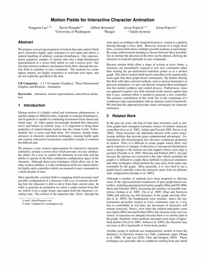
weight: weight:

BA

Figure 1: Control using action weights. By reweighting theneighbors (black dots) of our current state (white dot), we can con-trol motion synthesis to direct our character towards different nextstates (dashed dots).

4 Control

As described in section 3, at each possible state of the character amotion field there is a set of actions which the character can choosefrom in order to determine their motion over the next frame. Ingeneral, which particular action from this set it is best to choosedepends on the user’s current commands. Deciding on which actionto choose in each state in response to a user’s commands is thus keyin enabling real time interactive locomotion controllers.

4.1 Markov Decision Processes Control

A Markov decision process is a mathematical structure formalizingthe concept of making decisions in light of both their immediateand long-term results. An MDP consists of four parts: (1) a statespace, (2) actions to perform at each state, (3) a means of deter-mining the state transition produced by an action, and (4) rewardsfor occupying desired states and performing desired actions. Byexpressing character animation tasks in this framework, we makeour characters aware of long term consequences of their actions.This is useful even in graph-based controllers, but vital for motionfield controllers because we are acting every frame rather than everyclip. For further background on MDP-based control see [Sutton andBarto 1998], or [Treuille et al. 2007] and [Lo and Zwicker 2008] fortheir use in graph-based locomotion controllers.

States Simply representing the state of a character as a motionstate m is insufficient for interactive control, because we must alsorepresent how well the character is achieving its user-specified task.We therefore add a vector of task parameters θT to keep track ofhow well the task is being performed, forming joint task states s =(m, θT ). For instance in our direction following task θT records asingle number: the angular deviation from the desired heading. Byaltering this value, the user controls the character’s direction.

Actions At each task state s = (m, θT ) a character in a motionfield has a set of actionsA(m) to choose from in order to determinehow they will move over the next frame (section 3). There are in-finitely many different actions inA(m), but many of the techniquesused to solve MDPs require a finite set of actions at each state. Inorder to satisfy this requirement for our MDP controller, we samplea finite set of actions A(s) from A(m). Given a motion state m,we generate k actions by modifying the similarity weights (Equa-tion (2)). Each action is designed to prefer one neighbor over theothers.

{ ai

‖ai‖|ai = (w0, · · · , wi−1, 1, wi+1, · · · , wk−1)} (8)

In words, to derive action ai simply set wi to 1 and renormal-ize. This scheme samples actions which are not too different fromthe passive action at m so as to as to avoid jerkiness in the mo-tion, while giving the character enough flexibility to move towardsnearby motion states.

Transitions Additionally, we must extend the definition of theintegration function I (Equation (3)) to address task parameters:Is(s, a) = Is(m, θT , a) = (I(m,a), θ′T ). How to update taskparameters is normally obvious. For instance in the direction fol-lowing task, where θT is the characters deviation from the desireddirection, we simply adjust θT by the angle the character turned.

Rewards In order to make our character perform the desired taskwe offer rewards. Formally, a reward function specifies a real num-ber R(s, a) quantifying the reward received for performing the ac-tion a at state s. For instance, in our direction following task we

give high a high reward R(s, a) for maintaining a small deviationfrom the desired heading and a lower reward for large deviations.See section Section 6 for the specific task parameters and rewardfunctions we use in our demos.

4.2 Reinforcement Learning

The goal of reinforcement learning is to find “the best” rule or pol-icy for choosing which action to perform at any given state. A naıveapproach to this problem would be to pick the action which yieldsthe largest immediate reward: the greedy policy.

πG(s) = argmaxa∈A(s)

R(s, a) (9)

Although simple, this policy is myopic, ignoring the future ramifi-cations of each action choice. We already know that greedy graph-based controllers perform poorly [Treuille et al. 2007]. Motionfields are even worse. Even for the simple task of changing di-rection, we need a much longer horizon than 1

30th of a second to

anticipate and execute a turn.

Somehow, we need to consider the affect of the current actionchoice on the character’s ability to accrue future rewards. A looka-head policy πL does just this by considering the cumulative rewardover future task states:

πL(s) = argmaxa∈A(m)

"R(s, a) + max

{at}

∞Xt=1

γtR(st, at)

#(10)

with s1 = Is(s, a) and st = Is(st−1, at−1). γ is called the dis-count factor and controls how much the character focuses on shortterm (γ → 0) versus long term (γ → 1) reward.

As written, computing the lookahead policy involves solving for notonly the optimal next action, but also an infinite sequence of optimalfuture actions. Despite this apparent impracticality, a standard trickallows us to efficiently solve for the correct next action. The trickbegins by defining a value funciton V (s), a scalar-valued functionrepresenting the expected cumulative future reward received for act-ing optimally starting from task state s.

V (s) = maxa∈A(m)

∞Xt=0

γR(st, at) (11)

We will describe shortly how we represent and precompute thevalue function, but for the moment notice that we can now rewriteequation 8 by replacing the infinite future search with a value func-tion lookup:

πL(s) = argmaxa∈A(m)

[R(s, a) + V (Is(s, a))] (12)

Now the lookahead policy is only marginally more expensive tocompute than the greedy policy.

4.2.1 Value Function Representation and Learning

Since there are infinitely many possible task states, we cannot rep-resent the value function exactly. Instead we approximate it by stor-ing values at a finite number of task states si and interpolating toestimate the value at other points (Figure 2). We choose these taskstate samples by taking the Cartesian product of the database mo-tion states mi and a uniform grid sampling across the problem’stask parameters. See Section 6 for details of the sampling. Thissampling gives us high resolution near the motion database states,

CB

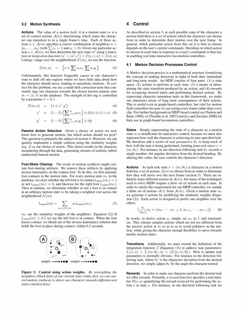
value: value:next state?

A

Figure 2: Action search using a value function. (A) At everystate, we have several possible actions (dashed lines) and their nextstates (dashed circles). (B) We interpolate the value function storedat database states (black points) to determine the value of each nextstate. (C) We select the highest value action to perform.

which is where the character generally stays. In order to calcu-late the value V (s) of a task state not in the database, we interpo-late over neighboring motion states using the similarity weights andover the task parameters multilinearly.

Given an MDP derived from a motion field and a task specification,we solve for an approximate value function in this form using fittedvalue iteration [Ernst et al. 2005]. Fitted value iteration operatesby first noting that equation 10 can be used to write the definitionof the value function in a recursive form. We express the value at atask state sample si recursively in terms of the value at other taskstate samples:

V (si) = R(si, πL(si)) + V (Is(si, πL(si))) (13)

where πL(si) is as defined in equation 10 and V (Is(si, a)) is com-puted via interpolation. We can solve for V (si) at each sample stateby iteratively applying equations 10 and 11. We begin with an all-zero value function V0(si) = 0 for each sample si. Then at each si

equation 10 is used to compute πL(s) after which we use equation11 to determine an updated value at si. After all the si samples havebeen processed in this manner, we have an updated approximationof the value function. We repeat this process until convergence anduse the last iteration as the final value function.

4.2.2 Temporal Value Function Compression

Unlike graph-based approaches, motion fields let characters be inconstant transition between many sources of data. Consequently,we need access to the value function at all motion states, ratherthan only at transitions between clips. This fact leads to a largememory footprint relative to graphs. We offset this weakness withcompression.

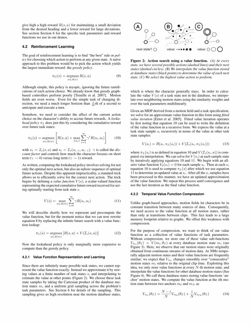
For the purpose of compression, we want to think of our valuefunction as a collection of value functions of task parameters.Without compression, we store one of these value sub-functionsVmi(θT ) = V (mi, θT ) at every database motion state mi (seeFigure 3). Here, we observe that our motion states were originallyobtained from continuous streams of motion data. At 30Hz tempo-rally adjacent motion states and their value functions are frequentlysimilar; we expect that Vmt changes smoothly over “consecutive”motion states mt relative to the original clip time. Exploiting thisidea, we only store value functions at every N -th motion state, andinterpolate the value functions for other database motion states (SeeFigure 4). We call these database states storing value functions ‘an-chor’ motion states. We compute the value function at the ith mo-tion state between two anchors m0 and mN as

Vmi(θT ) =N − iN

Vm0(θT ) +i

NVmN (θT ) (14)

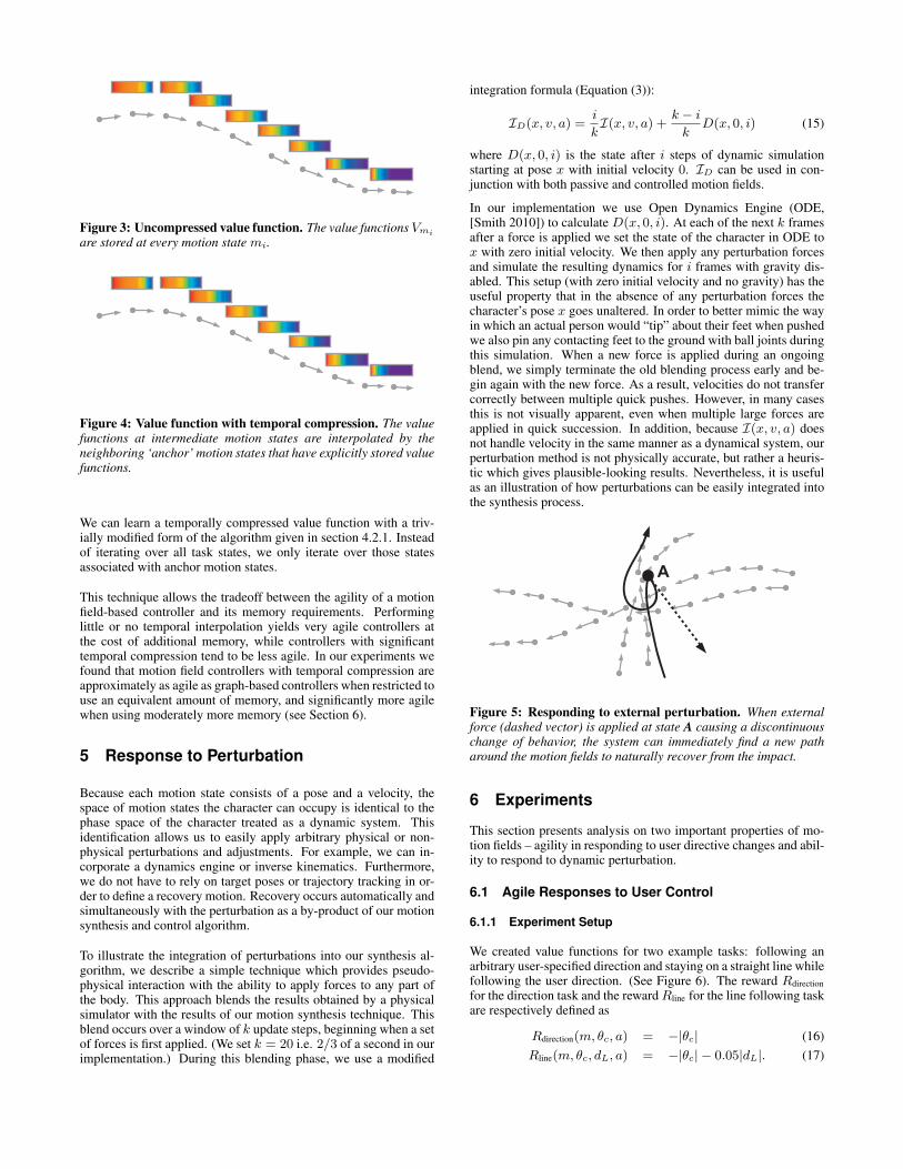
Figure 3: Uncompressed value function. The value functions Vmi

are stored at every motion state mi.

Figure 4: Value function with temporal compression. The valuefunctions at intermediate motion states are interpolated by theneighboring ‘anchor’ motion states that have explicitly stored valuefunctions.

We can learn a temporally compressed value function with a triv-ially modified form of the algorithm given in section 4.2.1. Insteadof iterating over all task states, we only iterate over those statesassociated with anchor motion states.

This technique allows the tradeoff between the agility of a motionfield-based controller and its memory requirements. Performinglittle or no temporal interpolation yields very agile controllers atthe cost of additional memory, while controllers with significanttemporal compression tend to be less agile. In our experiments wefound that motion field controllers with temporal compression areapproximately as agile as graph-based controllers when restricted touse an equivalent amount of memory, and significantly more agilewhen using moderately more memory (see Section 6).

5 Response to Perturbation

Because each motion state consists of a pose and a velocity, thespace of motion states the character can occupy is identical to thephase space of the character treated as a dynamic system. Thisidentification allows us to easily apply arbitrary physical or non-physical perturbations and adjustments. For example, we can in-corporate a dynamics engine or inverse kinematics. Furthermore,we do not have to rely on target poses or trajectory tracking in or-der to define a recovery motion. Recovery occurs automatically andsimultaneously with the perturbation as a by-product of our motionsynthesis and control algorithm.

To illustrate the integration of perturbations into our synthesis al-gorithm, we describe a simple technique which provides pseudo-physical interaction with the ability to apply forces to any part ofthe body. This approach blends the results obtained by a physicalsimulator with the results of our motion synthesis technique. Thisblend occurs over a window of k update steps, beginning when a setof forces is first applied. (We set k = 20 i.e. 2/3 of a second in ourimplementation.) During this blending phase, we use a modified

integration formula (Equation (3)):

ID(x, v, a) =i

kI(x, v, a) +

k − ik

D(x, 0, i) (15)

where D(x, 0, i) is the state after i steps of dynamic simulationstarting at pose x with initial velocity 0. ID can be used in con-junction with both passive and controlled motion fields.

In our implementation we use Open Dynamics Engine (ODE,[Smith 2010]) to calculate D(x, 0, i). At each of the next k framesafter a force is applied we set the state of the character in ODE tox with zero initial velocity. We then apply any perturbation forcesand simulate the resulting dynamics for i frames with gravity dis-abled. This setup (with zero initial velocity and no gravity) has theuseful property that in the absence of any perturbation forces thecharacter’s pose x goes unaltered. In order to better mimic the wayin which an actual person would “tip” about their feet when pushedwe also pin any contacting feet to the ground with ball joints duringthis simulation. When a new force is applied during an ongoingblend, we simply terminate the old blending process early and be-gin again with the new force. As a result, velocities do not transfercorrectly between multiple quick pushes. However, in many casesthis is not visually apparent, even when multiple large forces areapplied in quick succession. In addition, because I(x, v, a) doesnot handle velocity in the same manner as a dynamical system, ourperturbation method is not physically accurate, but rather a heuris-tic which gives plausible-looking results. Nevertheless, it is usefulas an illustration of how perturbations can be easily integrated intothe synthesis process.

A

Figure 5: Responding to external perturbation. When externalforce (dashed vector) is applied at state A causing a discontinuouschange of behavior, the system can immediately find a new patharound the motion fields to naturally recover from the impact.

6 Experiments

This section presents analysis on two important properties of mo-tion fields – agility in responding to user directive changes and abil-ity to respond to dynamic perturbation.

6.1 Agile Responses to User Control

6.1.1 Experiment Setup

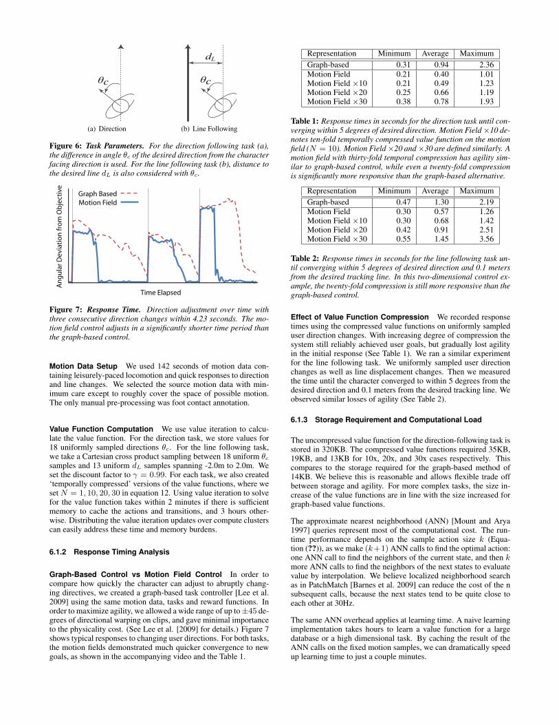
We created value functions for two example tasks: following anarbitrary user-specified direction and staying on a straight line whilefollowing the user direction. (See Figure 6). The reward Rdirectionfor the direction task and the rewardRline for the line following taskare respectively defined as

Rdirection(m, θc, a) = −|θc| (16)Rline(m, θc, dL, a) = −|θc| − 0.05|dL|. (17)

c

(a) Direction

c

dL

(b) Line Following

Figure 6: Task Parameters. For the direction following task (a),the difference in angle θc of the desired direction from the characterfacing direction is used. For the line following task (b), distance tothe desired line dL is also considered with θc.

Time Elapsed

An

gu

lar D

evia

tio

n fr

om

Ob

ject

ive

Graph BasedMotion Field

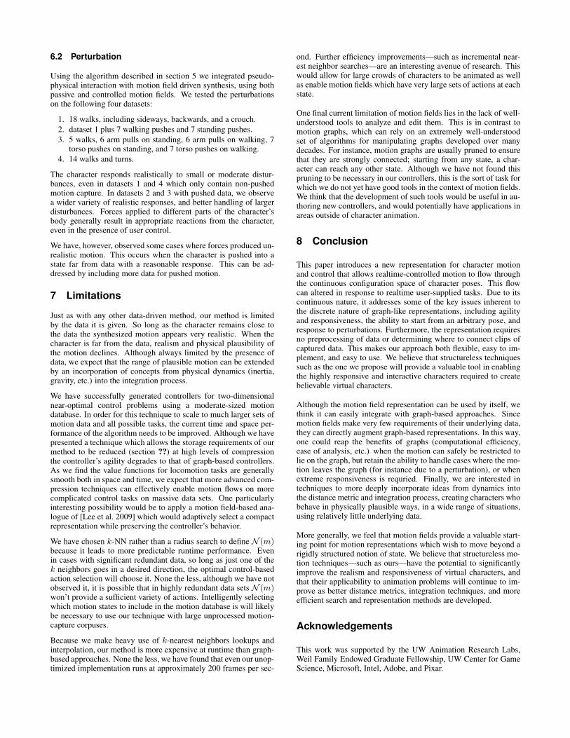
Figure 7: Response Time. Direction adjustment over time withthree consecutive direction changes within 4.23 seconds. The mo-tion field control adjusts in a significantly shorter time period thanthe graph-based control.

Motion Data Setup We used 142 seconds of motion data con-taining leisurely-paced locomotion and quick responses to directionand line changes. We selected the source motion data with min-imum care except to roughly cover the space of possible motion.The only manual pre-processing was foot contact annotation.

Value Function Computation We use value iteration to calcu-late the value function. For the direction task, we store values for18 uniformly sampled directions θc. For the line following task,we take a Cartesian cross product sampling between 18 uniform θc

samples and 13 uniform dL samples spanning -2.0m to 2.0m. Weset the discount factor to γ = 0.99. For each task, we also created‘temporally compressed’ versions of the value functions, where weset N = 1, 10, 20, 30 in equation 12. Using value iteration to solvefor the value function takes within 2 minutes if there is sufficientmemory to cache the actions and transitions, and 3 hours other-wise. Distributing the value iteration updates over compute clusterscan easily address these time and memory burdens.

6.1.2 Response Timing Analysis

Graph-Based Control vs Motion Field Control In order tocompare how quickly the character can adjust to abruptly chang-ing directives, we created a graph-based task controller [Lee et al.2009] using the same motion data, tasks and reward functions. Inorder to maximize agility, we allowed a wide range of up to±45 de-grees of directional warping on clips, and gave minimal importanceto the physicality cost. (See Lee et al. [2009] for details.) Figure 7shows typical responses to changing user directions. For both tasks,the motion fields demonstrated much quicker convergence to newgoals, as shown in the accompanying video and the Table 1.

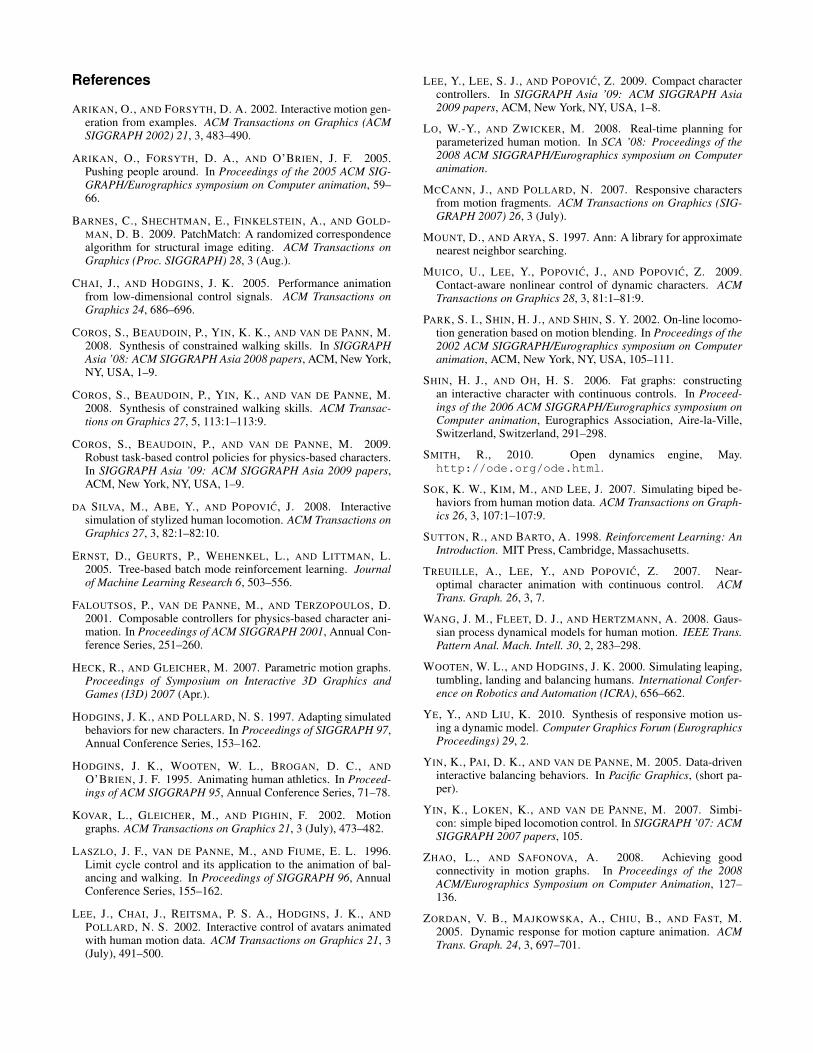
Representation Minimum Average MaximumGraph-based 0.31 0.94 2.36Motion Field 0.21 0.40 1.01Motion Field ×10 0.21 0.49 1.23Motion Field ×20 0.25 0.66 1.19Motion Field ×30 0.38 0.78 1.93

Table 1: Response times in seconds for the direction task until con-verging within 5 degrees of desired direction. Motion Field×10 de-notes ten-fold temporally compressed value function on the motionfield (N = 10). Motion Field×20 and×30 are defined similarly. Amotion field with thirty-fold temporal compression has agility sim-ilar to graph-based control, while even a twenty-fold compressionis significantly more responsive than the graph-based alternative.

Representation Minimum Average MaximumGraph-based 0.47 1.30 2.19Motion Field 0.30 0.57 1.26Motion Field ×10 0.30 0.68 1.42Motion Field ×20 0.42 0.91 2.51Motion Field ×30 0.55 1.45 3.56

Table 2: Response times in seconds for the line following task un-til converging within 5 degrees of desired direction and 0.1 metersfrom the desired tracking line. In this two-dimensional control ex-ample, the twenty-fold compression is still more responsive than thegraph-based control.

Effect of Value Function Compression We recorded responsetimes using the compressed value functions on uniformly sampleduser direction changes. With increasing degree of compression thesystem still reliably achieved user goals, but gradually lost agilityin the initial response (See Table 1). We ran a similar experimentfor the line following task. We uniformly sampled user directionchanges as well as line displacement changes. Then we measuredthe time until the character converged to within 5 degrees from thedesired direction and 0.1 meters from the desired tracking line. Weobserved similar losses of agility (See Table 2).

6.1.3 Storage Requirement and Computational Load

The uncompressed value function for the direction-following task isstored in 320KB. The compressed value functions required 35KB,19KB, and 13KB for 10x, 20x, and 30x cases respectively. Thiscompares to the storage required for the graph-based method of14KB. We believe this is reasonable and allows flexible trade offbetween storage and agility. For more complex tasks, the size in-crease of the value functions are in line with the size increased forgraph-based value functions.

The approximate nearest neighborhood (ANN) [Mount and Arya1997] queries represent most of the computational cost. The run-time performance depends on the sample action size k (Equa-tion (??)), as we make (k+1) ANN calls to find the optimal action:one ANN call to find the neighbors of the current state, and then kmore ANN calls to find the neighbors of the next states to evaluatevalue by interpolation. We believe localized neighborhood searchas in PatchMatch [Barnes et al. 2009] can reduce the cost of the nsubsequent calls, because the next states tend to be quite close toeach other at 30Hz.

The same ANN overhead applies at learning time. A naive learningimplementation takes hours to learn a value function for a largedatabase or a high dimensional task. By caching the result of theANN calls on the fixed motion samples, we can dramatically speedup learning time to just a couple minutes.

6.2 Perturbation

Using the algorithm described in section 5 we integrated pseudo-physical interaction with motion field driven synthesis, using bothpassive and controlled motion fields. We tested the perturbationson the following four datasets:

1. 18 walks, including sideways, backwards, and a crouch.2. dataset 1 plus 7 walking pushes and 7 standing pushes.3. 5 walks, 6 arm pulls on standing, 6 arm pulls on walking, 7

torso pushes on standing, and 7 torso pushes on walking.4. 14 walks and turns.

The character responds realistically to small or moderate distur-bances, even in datasets 1 and 4 which only contain non-pushedmotion capture. In datasets 2 and 3 with pushed data, we observea wider variety of realistic responses, and better handling of largerdisturbances. Forces applied to different parts of the character’sbody generally result in appropriate reactions from the character,even in the presence of user control.

We have, however, observed some cases where forces produced un-realistic motion. This occurs when the character is pushed into astate far from data with a reasonable response. This can be ad-dressed by including more data for pushed motion.

7 Limitations

Just as with any other data-driven method, our method is limitedby the data it is given. So long as the character remains close tothe data the synthesized motion appears very realistic. When thecharacter is far from the data, realism and physical plausibility ofthe motion declines. Although always limited by the presence ofdata, we expect that the range of plausible motion can be extendedby an incorporation of concepts from physical dynamics (inertia,gravity, etc.) into the integration process.

We have successfully generated controllers for two-dimensionalnear-optimal control problems using a moderate-sized motiondatabase. In order for this technique to scale to much larger sets ofmotion data and all possible tasks, the current time and space per-formance of the algorithm needs to be improved. Although we havepresented a technique which allows the storage requirements of ourmethod to be reduced (section ??) at high levels of compressionthe controller’s agility degrades to that of graph-based controllers.As we find the value functions for locomotion tasks are generallysmooth both in space and time, we expect that more advanced com-pression techniques can effectively enable motion flows on morecomplicated control tasks on massive data sets. One particularlyinteresting possibility would be to apply a motion field-based ana-logue of [Lee et al. 2009] which would adaptively select a compactrepresentation while preserving the controller’s behavior.

We have chosen k-NN rather than a radius search to define N (m)because it leads to more predictable runtime performance. Evenin cases with significant redundant data, so long as just one of thek neighbors goes in a desired direction, the optimal control-basedaction selection will choose it. None the less, although we have notobserved it, it is possible that in highly redundant data sets N (m)won’t provide a sufficient variety of actions. Intelligently selectingwhich motion states to include in the motion database is will likelybe necessary to use our technique with large unprocessed motion-capture corpuses.

Because we make heavy use of k-nearest neighbors lookups andinterpolation, our method is more expensive at runtime than graph-based approaches. None the less, we have found that even our unop-timized implementation runs at approximately 200 frames per sec-

ond. Further efficiency improvements—such as incremental near-est neighbor searches—are an interesting avenue of research. Thiswould allow for large crowds of characters to be animated as wellas enable motion fields which have very large sets of actions at eachstate.

One final current limitation of motion fields lies in the lack of well-understood tools to analyze and edit them. This is in contrast tomotion graphs, which can rely on an extremely well-understoodset of algorithms for manipulating graphs developed over manydecades. For instance, motion graphs are usually pruned to ensurethat they are strongly connected; starting from any state, a char-acter can reach any other state. Although we have not found thispruning to be necessary in our controllers, this is the sort of task forwhich we do not yet have good tools in the context of motion fields.We think that the development of such tools would be useful in au-thoring new controllers, and would potentially have applications inareas outside of character animation.

8 Conclusion

This paper introduces a new representation for character motionand control that allows realtime-controlled motion to flow throughthe continuous configuration space of character poses. This flowcan altered in response to realtime user-supplied tasks. Due to itscontinuous nature, it addresses some of the key issues inherent tothe discrete nature of graph-like representations, including agilityand responsiveness, the ability to start from an arbitrary pose, andresponse to perturbations. Furthermore, the representation requiresno preprocessing of data or determining where to connect clips ofcaptured data. This makes our approach both flexible, easy to im-plement, and easy to use. We believe that structureless techniquessuch as the one we propose will provide a valuable tool in enablingthe highly responsive and interactive characters required to createbelievable virtual characters.

Although the motion field representation can be used by itself, wethink it can easily integrate with graph-based approaches. Sincemotion fields make very few requirements of their underlying data,they can directly augment graph-based representations. In this way,one could reap the benefits of graphs (computational efficiency,ease of analysis, etc.) when the motion can safely be restricted tolie on the graph, but retain the ability to handle cases where the mo-tion leaves the graph (for instance due to a perturbation), or whenextreme responsiveness is requried. Finally, we are interested intechniques to more deeply incorporate ideas from dynamics intothe distance metric and integration process, creating characters whobehave in physically plausible ways, in a wide range of situations,using relatively little underlying data.

More generally, we feel that motion fields provide a valuable start-ing point for motion representations which wish to move beyond arigidly structured notion of state. We believe that structureless mo-tion techniques—such as ours—have the potential to significantlyimprove the realism and responsiveness of virtual characters, andthat their applicability to animation problems will continue to im-prove as better distance metrics, integration techniques, and moreefficient search and representation methods are developed.

Acknowledgements

This work was supported by the UW Animation Research Labs,Weil Family Endowed Graduate Fellowship, UW Center for GameScience, Microsoft, Intel, Adobe, and Pixar.

References

ARIKAN, O., AND FORSYTH, D. A. 2002. Interactive motion gen-eration from examples. ACM Transactions on Graphics (ACMSIGGRAPH 2002) 21, 3, 483–490.

ARIKAN, O., FORSYTH, D. A., AND O’BRIEN, J. F. 2005.Pushing people around. In Proceedings of the 2005 ACM SIG-GRAPH/Eurographics symposium on Computer animation, 59–66.

BARNES, C., SHECHTMAN, E., FINKELSTEIN, A., AND GOLD-MAN, D. B. 2009. PatchMatch: A randomized correspondencealgorithm for structural image editing. ACM Transactions onGraphics (Proc. SIGGRAPH) 28, 3 (Aug.).

CHAI, J., AND HODGINS, J. K. 2005. Performance animationfrom low-dimensional control signals. ACM Transactions onGraphics 24, 686–696.

COROS, S., BEAUDOIN, P., YIN, K. K., AND VAN DE PANN, M.2008. Synthesis of constrained walking skills. In SIGGRAPHAsia ’08: ACM SIGGRAPH Asia 2008 papers, ACM, New York,NY, USA, 1–9.

COROS, S., BEAUDOIN, P., YIN, K., AND VAN DE PANNE, M.2008. Synthesis of constrained walking skills. ACM Transac-tions on Graphics 27, 5, 113:1–113:9.

COROS, S., BEAUDOIN, P., AND VAN DE PANNE, M. 2009.Robust task-based control policies for physics-based characters.In SIGGRAPH Asia ’09: ACM SIGGRAPH Asia 2009 papers,ACM, New York, NY, USA, 1–9.

DA SILVA, M., ABE, Y., AND POPOVIC, J. 2008. Interactivesimulation of stylized human locomotion. ACM Transactions onGraphics 27, 3, 82:1–82:10.

ERNST, D., GEURTS, P., WEHENKEL, L., AND LITTMAN, L.2005. Tree-based batch mode reinforcement learning. Journalof Machine Learning Research 6, 503–556.

FALOUTSOS, P., VAN DE PANNE, M., AND TERZOPOULOS, D.2001. Composable controllers for physics-based character ani-mation. In Proceedings of ACM SIGGRAPH 2001, Annual Con-ference Series, 251–260.

HECK, R., AND GLEICHER, M. 2007. Parametric motion graphs.Proceedings of Symposium on Interactive 3D Graphics andGames (I3D) 2007 (Apr.).

HODGINS, J. K., AND POLLARD, N. S. 1997. Adapting simulatedbehaviors for new characters. In Proceedings of SIGGRAPH 97,Annual Conference Series, 153–162.

HODGINS, J. K., WOOTEN, W. L., BROGAN, D. C., ANDO’BRIEN, J. F. 1995. Animating human athletics. In Proceed-ings of ACM SIGGRAPH 95, Annual Conference Series, 71–78.

KOVAR, L., GLEICHER, M., AND PIGHIN, F. 2002. Motiongraphs. ACM Transactions on Graphics 21, 3 (July), 473–482.

LASZLO, J. F., VAN DE PANNE, M., AND FIUME, E. L. 1996.Limit cycle control and its application to the animation of bal-ancing and walking. In Proceedings of SIGGRAPH 96, AnnualConference Series, 155–162.

LEE, J., CHAI, J., REITSMA, P. S. A., HODGINS, J. K., ANDPOLLARD, N. S. 2002. Interactive control of avatars animatedwith human motion data. ACM Transactions on Graphics 21, 3(July), 491–500.

LEE, Y., LEE, S. J., AND POPOVIC, Z. 2009. Compact charactercontrollers. In SIGGRAPH Asia ’09: ACM SIGGRAPH Asia2009 papers, ACM, New York, NY, USA, 1–8.

LO, W.-Y., AND ZWICKER, M. 2008. Real-time planning forparameterized human motion. In SCA ’08: Proceedings of the2008 ACM SIGGRAPH/Eurographics symposium on Computeranimation.

MCCANN, J., AND POLLARD, N. 2007. Responsive charactersfrom motion fragments. ACM Transactions on Graphics (SIG-GRAPH 2007) 26, 3 (July).

MOUNT, D., AND ARYA, S. 1997. Ann: A library for approximatenearest neighbor searching.

MUICO, U., LEE, Y., POPOVIC, J., AND POPOVIC, Z. 2009.Contact-aware nonlinear control of dynamic characters. ACMTransactions on Graphics 28, 3, 81:1–81:9.

PARK, S. I., SHIN, H. J., AND SHIN, S. Y. 2002. On-line locomo-tion generation based on motion blending. In Proceedings of the2002 ACM SIGGRAPH/Eurographics symposium on Computeranimation, ACM, New York, NY, USA, 105–111.

SHIN, H. J., AND OH, H. S. 2006. Fat graphs: constructingan interactive character with continuous controls. In Proceed-ings of the 2006 ACM SIGGRAPH/Eurographics symposium onComputer animation, Eurographics Association, Aire-la-Ville,Switzerland, Switzerland, 291–298.

SMITH, R., 2010. Open dynamics engine, May.http://ode.org/ode.html.

SOK, K. W., KIM, M., AND LEE, J. 2007. Simulating biped be-haviors from human motion data. ACM Transactions on Graph-ics 26, 3, 107:1–107:9.

SUTTON, R., AND BARTO, A. 1998. Reinforcement Learning: AnIntroduction. MIT Press, Cambridge, Massachusetts.

TREUILLE, A., LEE, Y., AND POPOVIC, Z. 2007. Near-optimal character animation with continuous control. ACMTrans. Graph. 26, 3, 7.

WANG, J. M., FLEET, D. J., AND HERTZMANN, A. 2008. Gaus-sian process dynamical models for human motion. IEEE Trans.Pattern Anal. Mach. Intell. 30, 2, 283–298.

WOOTEN, W. L., AND HODGINS, J. K. 2000. Simulating leaping,tumbling, landing and balancing humans. International Confer-ence on Robotics and Automation (ICRA), 656–662.

YE, Y., AND LIU, K. 2010. Synthesis of responsive motion us-ing a dynamic model. Computer Graphics Forum (EurographicsProceedings) 29, 2.

YIN, K., PAI, D. K., AND VAN DE PANNE, M. 2005. Data-driveninteractive balancing behaviors. In Pacific Graphics, (short pa-per).

YIN, K., LOKEN, K., AND VAN DE PANNE, M. 2007. Simbi-con: simple biped locomotion control. In SIGGRAPH ’07: ACMSIGGRAPH 2007 papers, 105.

ZHAO, L., AND SAFONOVA, A. 2008. Achieving goodconnectivity in motion graphs. In Proceedings of the 2008ACM/Eurographics Symposium on Computer Animation, 127–136.

ZORDAN, V. B., MAJKOWSKA, A., CHIU, B., AND FAST, M.2005. Dynamic response for motion capture animation. ACMTrans. Graph. 24, 3, 697–701.