morphology 3 unsupervised morphology induction sudeshna sarkar iit kharagpur
TRANSCRIPT
Morphology 3Unsupervised Morphology Induction
Sudeshna Sarkar
IIT Kharagpur
Linguistica:Unsupervised Learning of Natural Language Morphology Using MDL
John GoldsmithDepartment of Linguistics The University of Chicago
Unsupervised learning
Input: untagged text in orthographic or phonetic form with spaces (or punctuation) separating words. But no tagging or text preparation.
Output List of stems, suffixes, and prefixes List of signatures.
A signature: a list of all suffixes (prefixes) appearing in a given corpus with a given stem.
Hence, a stem in a corpus has a unique signature. A signature has a unique set of stems associated with it
…
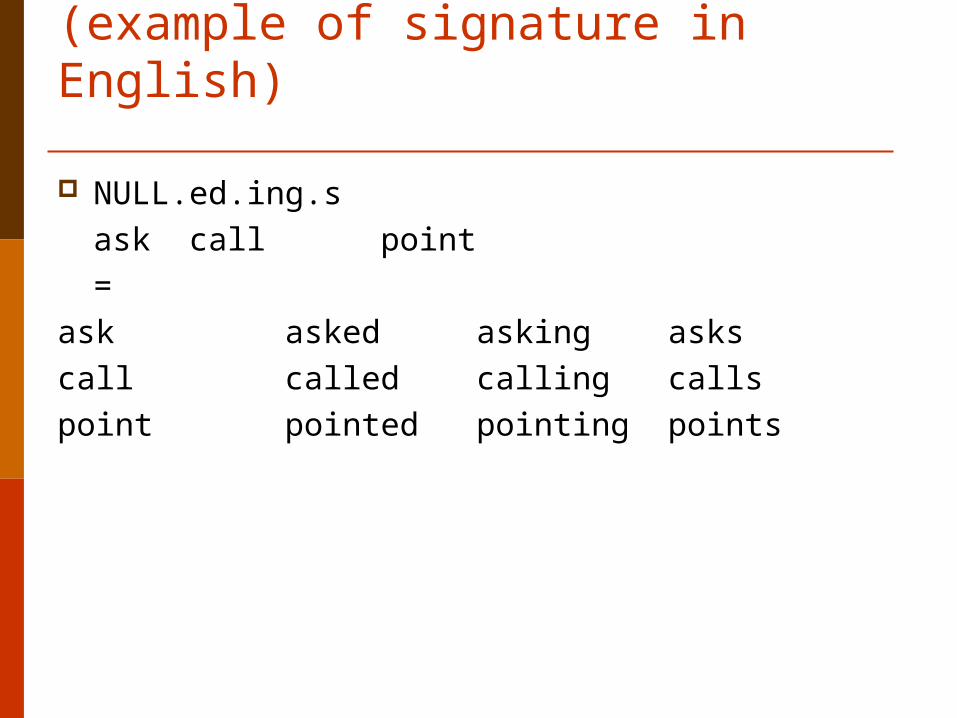
(example of signature in English)
NULL.ed.ing.s
ask call point
=
ask asked asking asks
call called calling calls
point pointed pointing points
…output
Roots (“stems of stems”) and the inner structure of stems
Regular allomorphy of stems:
e.g., learn “delete stem-final –e in English before –ing and –ed”
Essence of Minimum Description Length (MDL)
Jorma Rissanen: Stochastic Complexity in Statistical Inquiry (1989)
Work by Michael Brent and Carl de Marcken on word-discovery using MDL
We are given
1. a corpus, and
2. a probabilistic morphology, which technically means that we are given a distribution over certain strings of stems and affixes.
The higher the probability is that the morphology assigns to the (observed) corpus, the better that morphology is as a model of that data.
Better said: -1 * log probability (corpus) is a measure of how well the
morphology models the data: the smaller that number is, the better the morphology models the data.
This is known as the optimal compressed length of the data, given the model.
Using base 2 logs, this number is a measure in information theoretic bits.
Essence of MDL…
The goodness of the morphology is also measured by how compact the morphology is.
We can measure the compactness of a morphology in information theoretic bits.
How can we measure the compactness of a morphology?
Let’s consider a naïve version of description length: count the number of letters.
This naïve version is nonetheless helpful in seeing the intuition involved.
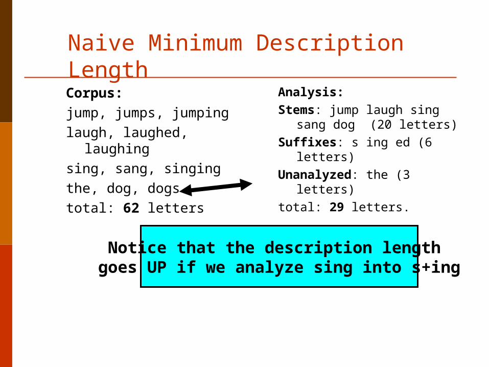
Naive Minimum Description Length
Corpus:
jump, jumps, jumping
laugh, laughed, laughing
sing, sang, singing
the, dog, dogs
total: 62 letters
Analysis:
Stems: jump laugh sing sang dog (20 letters)
Suffixes: s ing ed (6 letters)
Unanalyzed: the (3 letters)
total: 29 letters.
Notice that the description length goes UP if we analyze sing into s+ing
Essence of MDL…
The best overall theory of a corpus is the one for which the sum of
log prob (corpus) + length of the morphology
(that’s the description length) is the smallest.
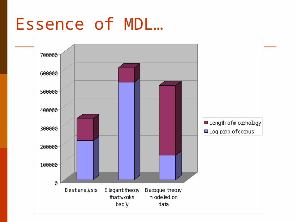
Essence of MDL…
0
100000
200000
300000
400000
500000
600000
700000
Best analysis Elegant theorythat works
badly
Baroque theorymodeled on
data
Length of morphology
Log prob of corpus
Overall logic
Search through morphology space for the morphology which provides the smallest description length.
1. Application of MDL to iterative search of morphology-space, with successively finer-grained descriptions
Corpus
Pick a large corpus from a language --5,000 to 1,000,000 words.
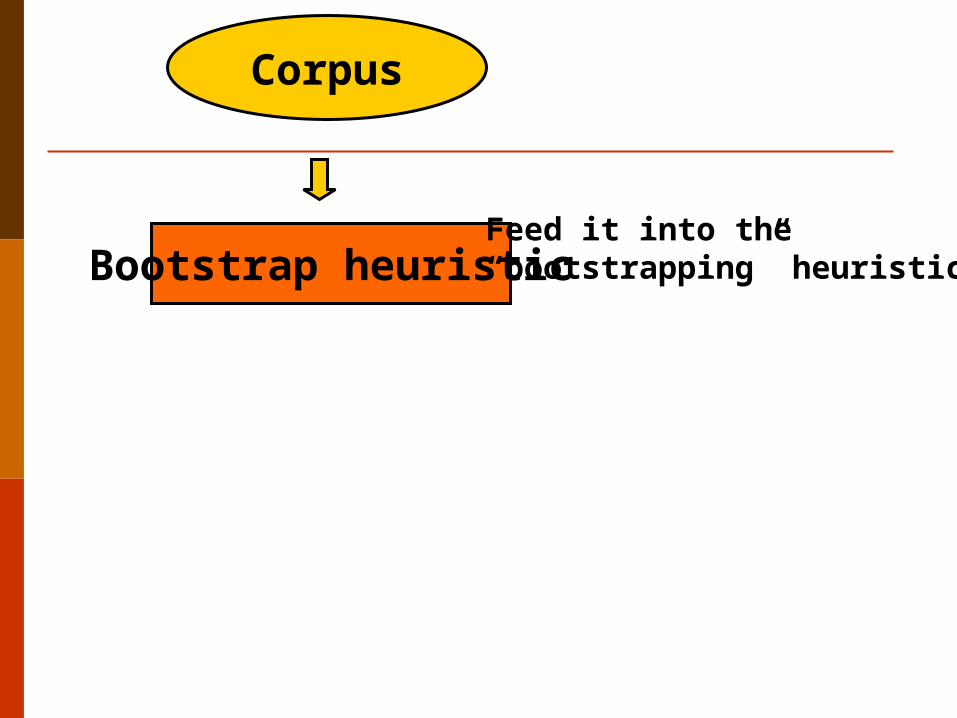
Corpus
Bootstrap heuristicFeed it into the “bootstrapping” heuristic...
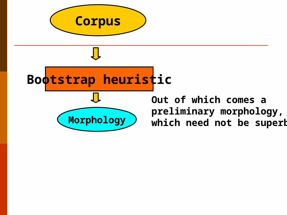
Corpus
Out of which comes a preliminary morphology,which need not be superb.Morphology
Bootstrap heuristic
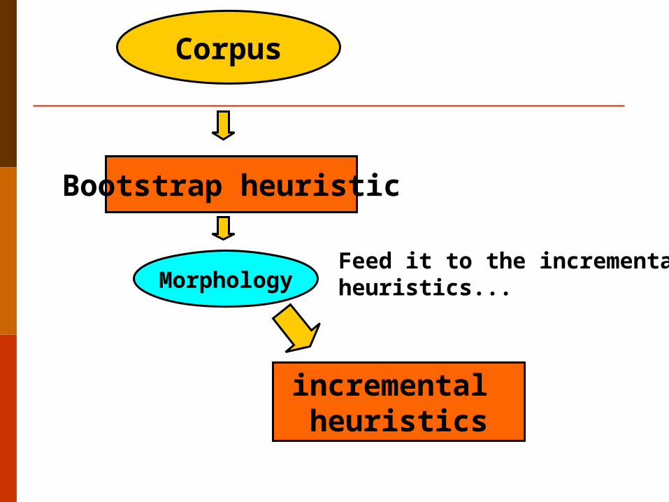
Corpus
Morphology
Bootstrap heuristic
incremental heuristics
Feed it to the incrementalheuristics...
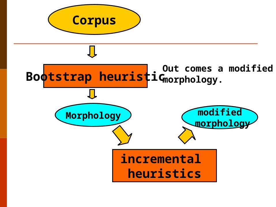
Corpus
Morphology
Bootstrap heuristic
incremental heuristics
modified morphology
Out comes a modifiedmorphology.
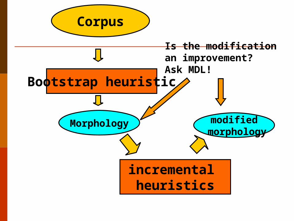
Corpus
Morphology
Bootstrap heuristic
incremental heuristics
modified morphology
Is the modificationan improvement?Ask MDL!
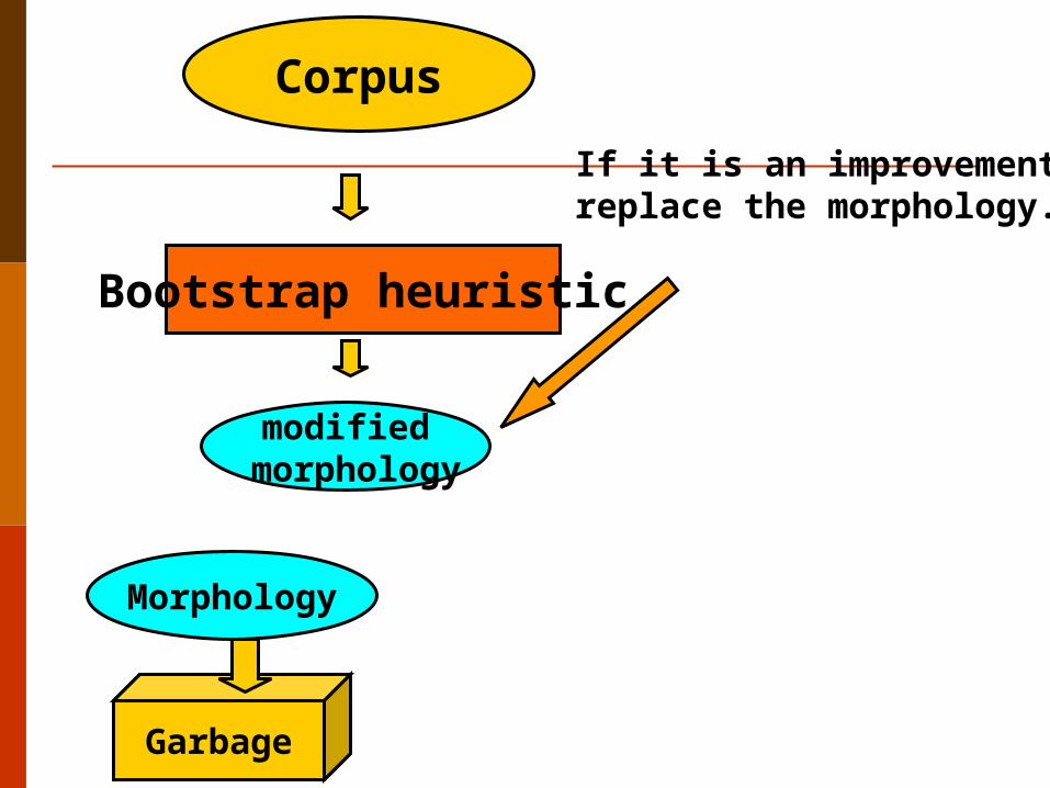
Corpus
Morphology
Bootstrap heuristic
modified morphology
If it is an improvement,replace the morphology...
Garbage
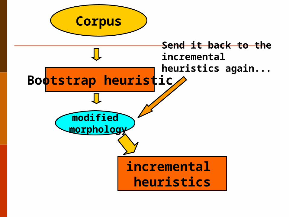
Corpus
Bootstrap heuristic
incremental heuristics
modified morphology
Send it back to theincremental heuristics again...
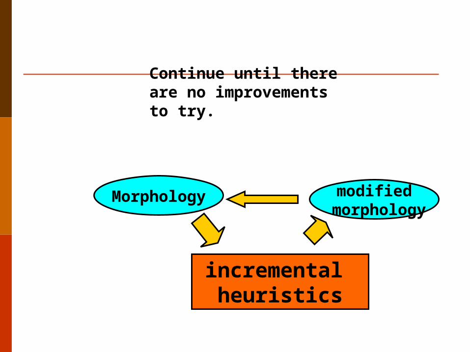
Morphology
incremental heuristics
modified morphology
Continue until there are no improvementsto try.
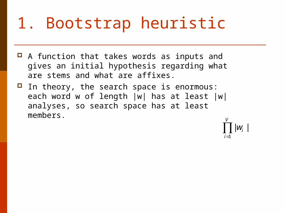
1. Bootstrap heuristic
A function that takes words as inputs and gives an initial hypothesis regarding what are stems and what are affixes.
In theory, the search space is enormous: each word w of length |w| has at least |w| analyses, so search space has at least members.
V
iiw
1
||
Better bootstrap heuristics
Heuristic, not perfection! Several good heuristics. Best is a modification of a good idea of Zellig Harris (1955):
Current variant:Cut words at certain peaks of successor frequency.
Problems: can over-cut; can under-cut; and can put cuts too far to the right (“aborti-” problem). [Not a problem!]
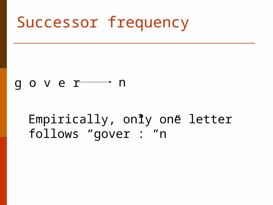
Successor frequency
g o v e r n
Empirically, only one letter follows “gover”: “n”
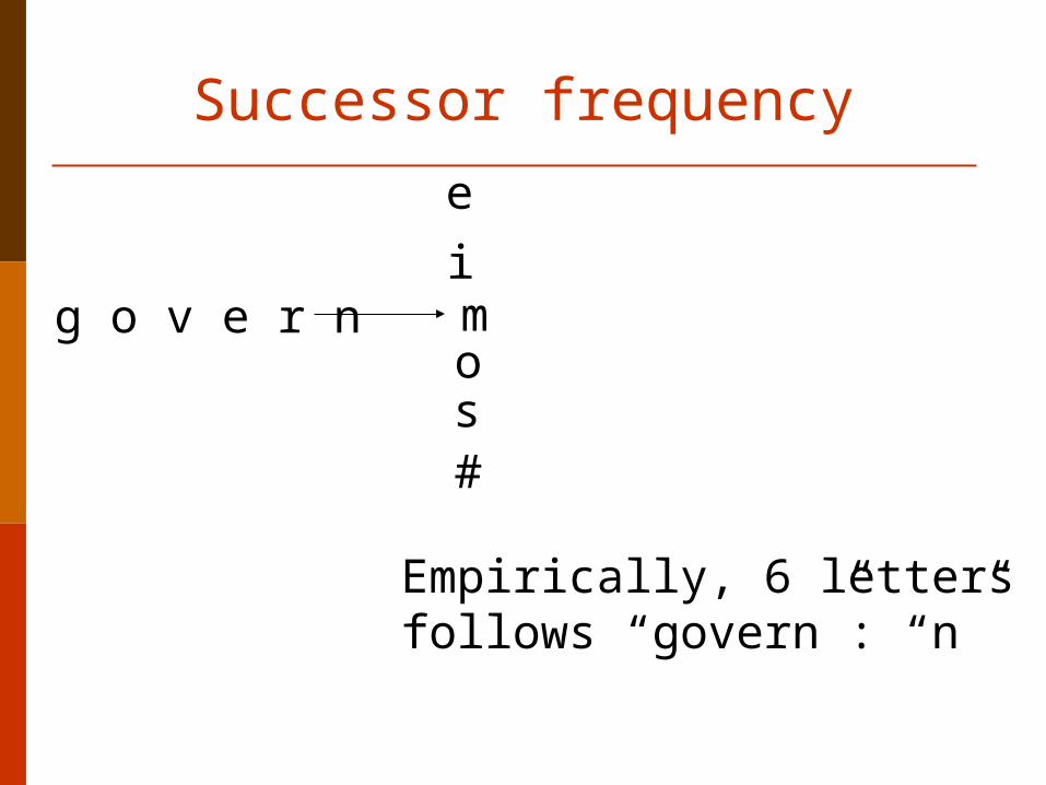
Successor frequency
g o v e r n m
Empirically, 6 letters follows “govern”: “n”
i
os
e
#
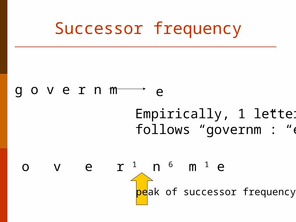
Successor frequency
g o v e r n m
Empirically, 1 letter follows “governm”: “e”
e
g o v e r 1 n 6 m 1 e
peak of successor frequency
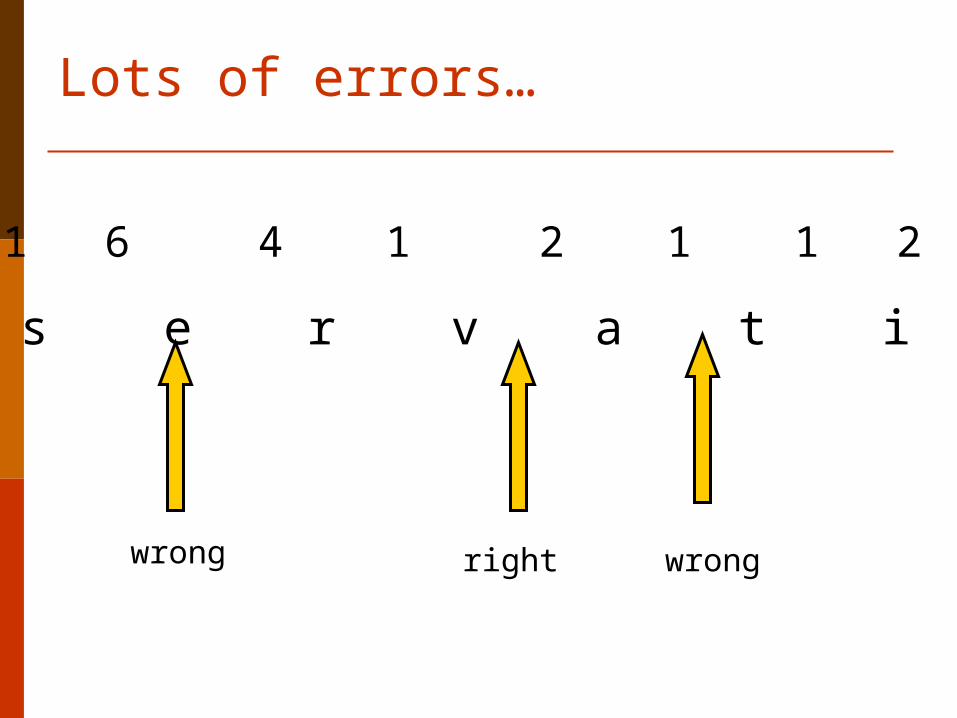
Lots of errors…
c o n s e r v a t i v e s
9 18 11 6 4 1 2 1 1 2 1 1
wrong right wrong
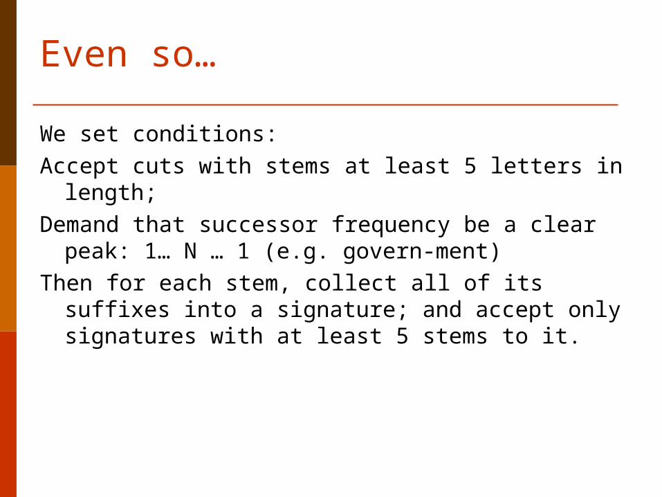
Even so…
We set conditions:
Accept cuts with stems at least 5 letters in length;
Demand that successor frequency be a clear peak: 1… N … 1 (e.g. govern-ment)
Then for each stem, collect all of its suffixes into a signature; and accept only signatures with at least 5 stems to it.
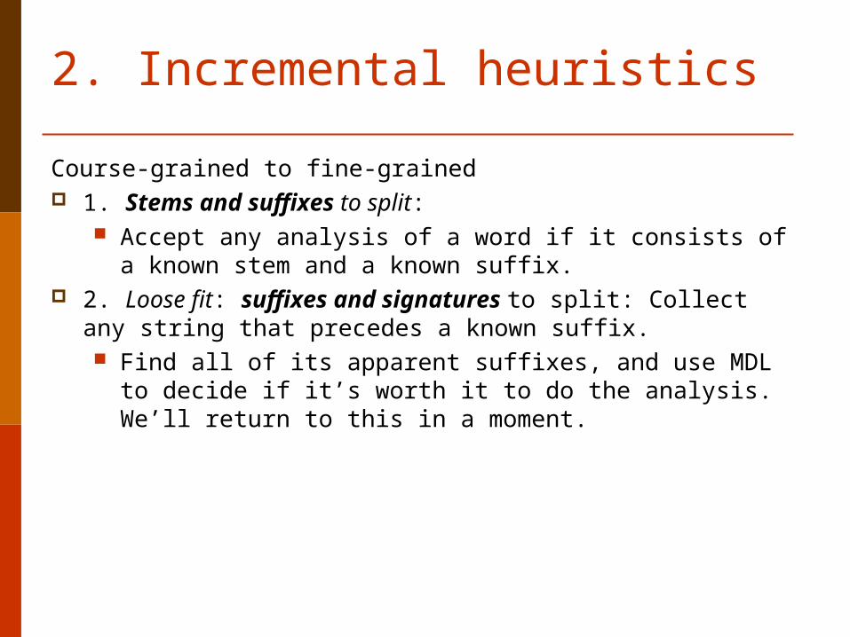
2. Incremental heuristics
Course-grained to fine-grained 1. Stems and suffixes to split:
Accept any analysis of a word if it consists of a known stem and a known suffix.
2. Loose fit: suffixes and signatures to split: Collect any string that precedes a known suffix. Find all of its apparent suffixes, and use MDL to decide if it’s
worth it to do the analysis. We’ll return to this in a moment.
Incremental heuristic
3.Slide stem-suffix boundary to the left: Again, use MDL to decide.
How do we use MDL to decide?
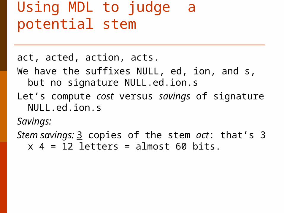
Using MDL to judge a potential stem
act, acted, action, acts.
We have the suffixes NULL, ed, ion, and s, but no signature NULL.ed.ion.s
Let’s compute cost versus savings of signature NULL.ed.ion.s
Savings:
Stem savings: 3 copies of the stem act: that’s 3 x 4 = 12 letters = almost 60 bits.
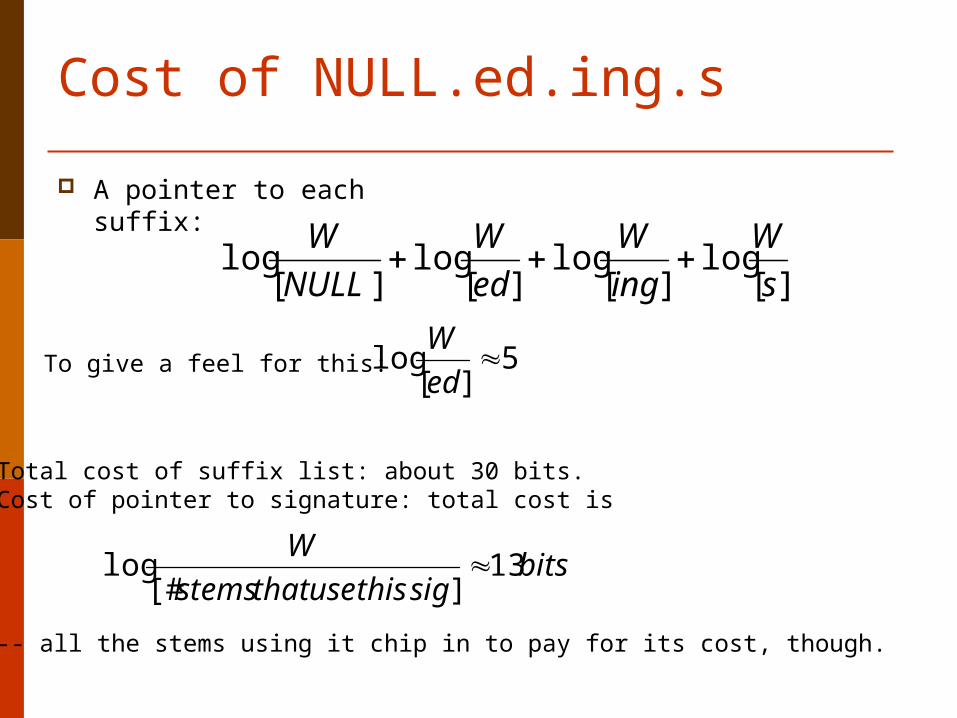
Cost of NULL.ed.ing.s
A pointer to each suffix:
][log
][log
][log
][log
s
W
ing
W
ed
W
NULL
W
To give a feel for this: 5][
log ed
W
Total cost of suffix list: about 30 bits.Cost of pointer to signature: total cost is
-- all the stems using it chip in to pay for its cost, though.
bitssigthisusethatstems
W13
][#log
Cost of signature: about 45 bits Savings: about 60 bits
so MDL says: Do it! Analyze the words as stem + suffix.
Notice that the cost of the analysis would have been higher if one or more of the suffixes had not already “existed”.
Today’s presentation
1. The task: unsupervised learning2. Overview of program and output3. Overview of Minimum Description Length framework4. Application of MDL to iterative search of morphology-
space, with successively finer-grained descriptions5. Mathematical model6. Current capabilities7. Current challenges
Model
A model to give us a probability of each word in the corpus (hence, its optimal compressed length); and
A morphology whose length we can measure.
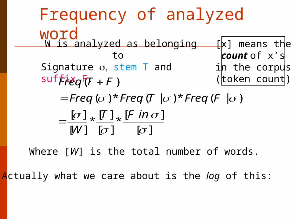
Frequency of analyzed word
][
][*
][
][*
][
][
)|(*)|(*)(
)(
inFT
W
FFreqTFreqFreq
FTFreq
W is analyzed as belonging to Signature stem T and suffix F.
Actually what we care about is the log of this:
Where [W] is the total number of words.
[x] means thecount of x’sin the corpus(token count)
][
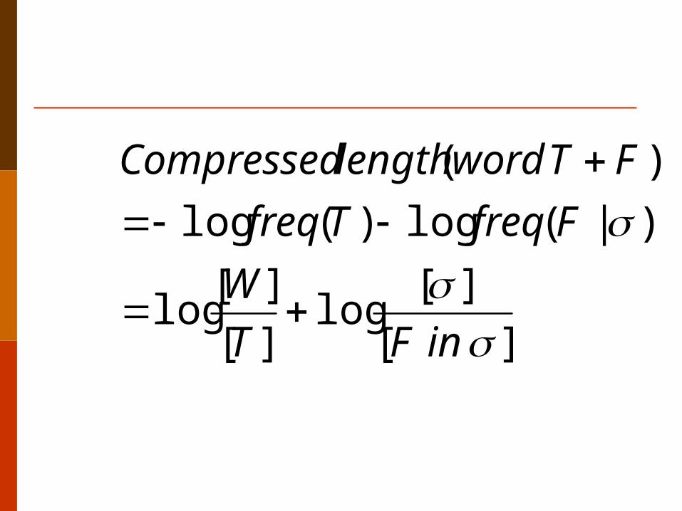
][log
][
][log
)|(log)(log
)(
inFT
W
FfreqTfreq
FTwordlengthCompressed
Next, let’s see how to measurethe length of a morphology
A morphology is a set of 3 things: A list of stems; A list of suffixes; A list of signatures with the associated stems.
We’ll make an effort to make our grammars consist primarily of lists, whose length is conceptually simple.
Length of a list
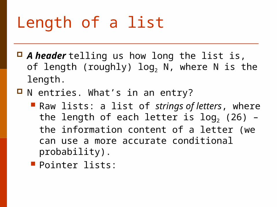
A header telling us how long the list is, of length (roughly) log2 N, where N is the length.
N entries. What’s in an entry? Raw lists: a list of strings of letters, where the length
of each letter is log2 (26) – the information content of a letter (we can use a more accurate conditional probability).
Pointer lists:
Lists
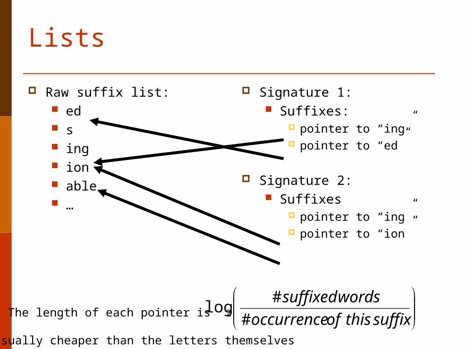
Raw suffix list: ed s ing ion able …
Signature 1: Suffixes:
pointer to “ing” pointer to “ed”
Signature 2: Suffixes
pointer to “ing” pointer to “ion”
The length of each pointer is
suffixthisofoccurrence
wordssuffixed
#
#log2
-- usually cheaper than the letters themselves
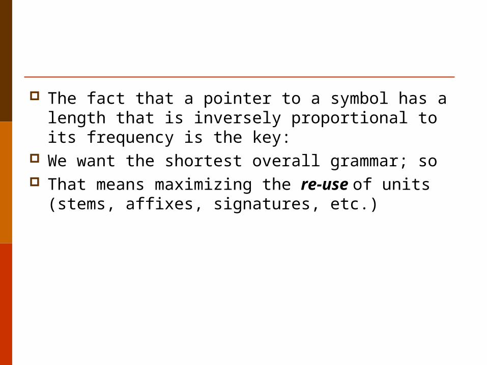
The fact that a pointer to a symbol has a length that is inversely proportional to its frequency is the key:
We want the shortest overall grammar; so That means maximizing the re-use of units (stems,
affixes, signatures, etc.)
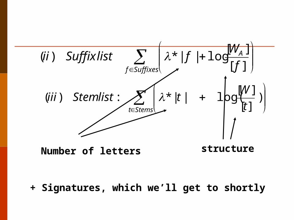
Suffixesf
A
f
WflistSuffixii
][
][log||*)(
Stemst t
WtlistStemiii )
][
][log(||*:)(
Number of letters structure
+ Signatures, which we’ll get to shortly
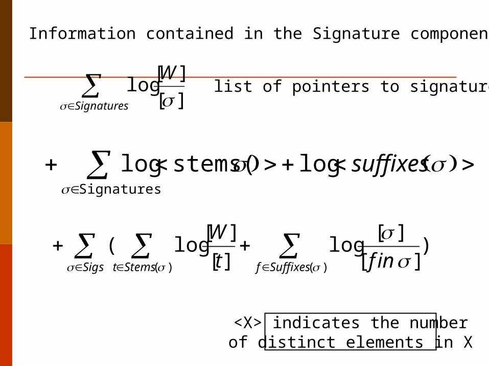
Information contained in the Signature component
Signatures
W
][
][log list of pointers to signatures
logstems( log Signatures
suffixes
)][
][log
][
][log(
)()(
SuffixesfSigs Stemst inft
W
<X> indicates the numberof distinct elements in X
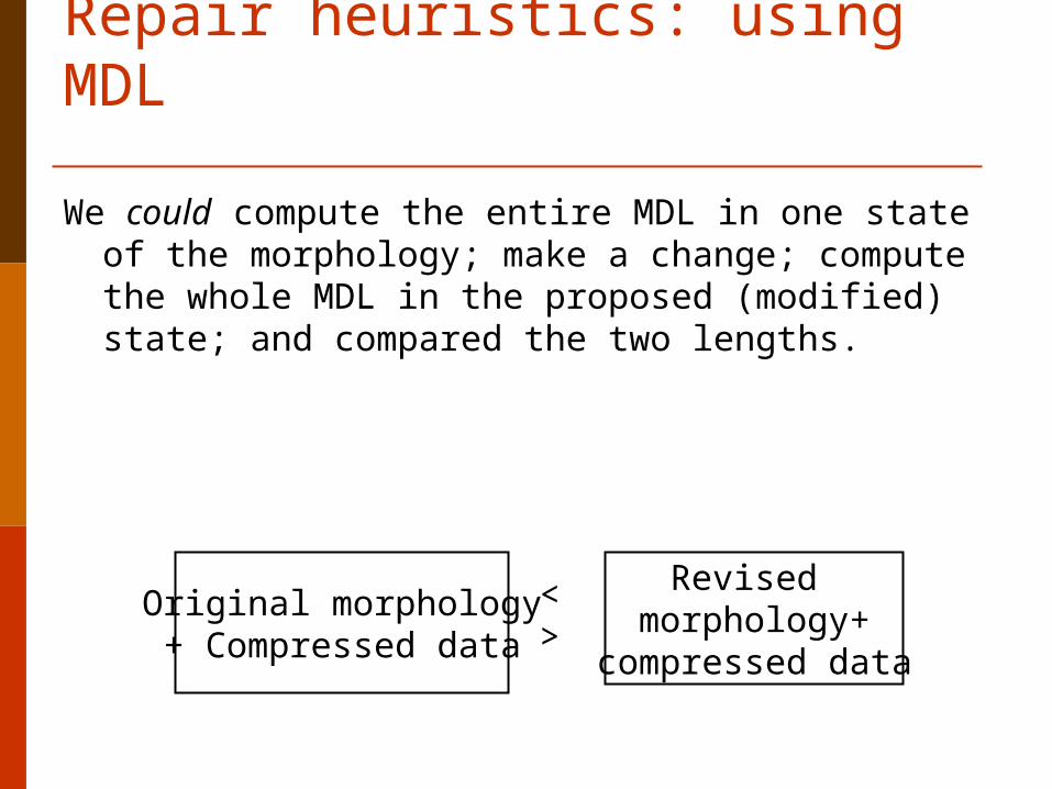
Original morphology+ Compressed data
Repair heuristics: using MDL
We could compute the entire MDL in one state of the morphology; make a change; compute the whole MDL in the proposed (modified) state; and compared the two lengths.
Revised morphology+
compressed data
<>
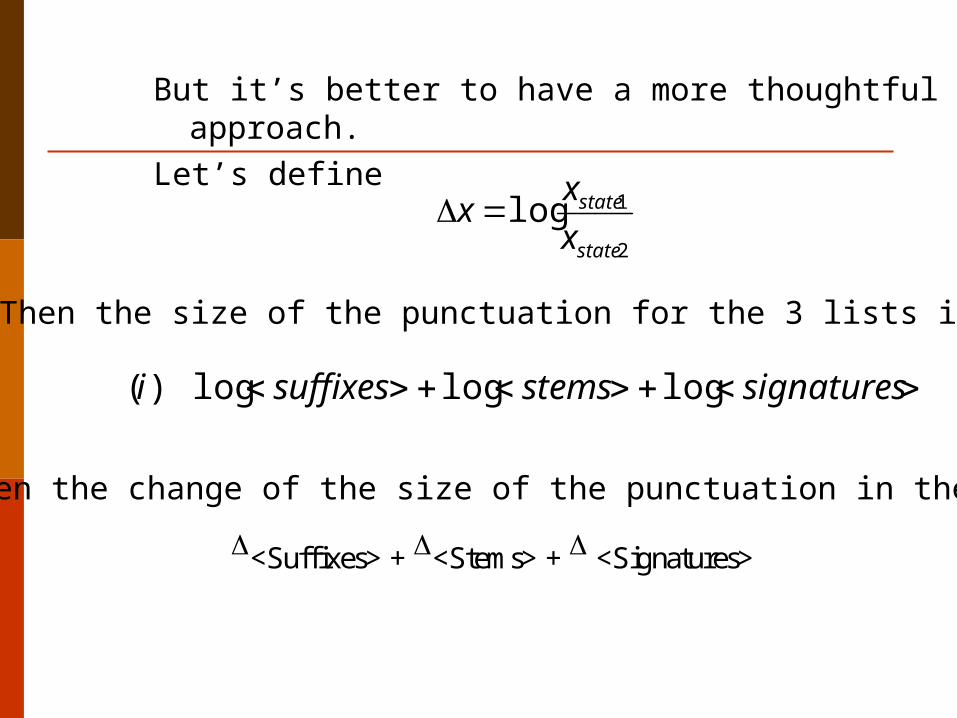
But it’s better to have a more thoughtful approach.
Let’s define
2
1logstate
state
x
xx
Then the change of the size of the punctuation in the lists:
signaturesstemssuffixesi logloglog)(
Then the size of the punctuation for the 3 lists is:
<Suffixes> + <Stems> + <Signatures>
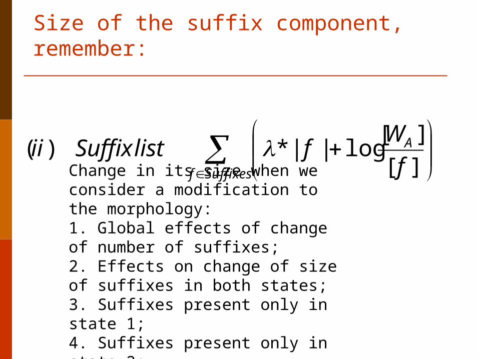
Size of the suffix component, remember:
Suffixesf
A
f
WflistSuffixii
][
][log||*)(
Change in its size when we consider a modification to the morphology:1. Global effects of change of number of suffixes;2. Effects on change of size of suffixes in both states;3. Suffixes present only in state 1;4. Suffixes present only in state 2;
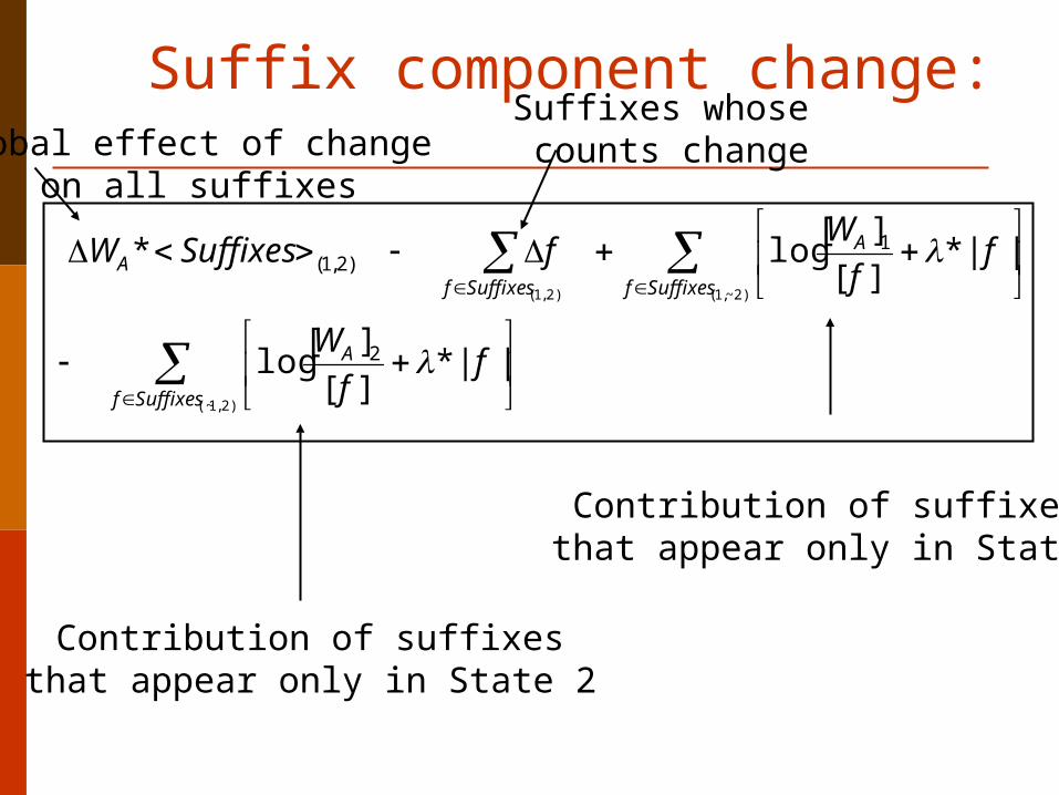
Suffix component change:
)2,1(~
)2~,1()2,1(
||*][
][log
||*][
][log*
2
1)2,1(
Suffixesf
A
Suffixesf
A
SuffixesfA
ff
W
ff
WfSuffixesW
Contribution of suffixesthat appear only in State1
Contribution of suffixesthat appear only in State 2
Global effect of change on all suffixes
Suffixes whose counts change
Current research projects
1. Allomorphy: Automatic discovery of relationship between stems (lov~love, win~winn)
2. Use of syntax (automatic learning of syntactic categories)
3. Rich morphology: other languages (e.g., Swahili), other sub-languages (e.g., biochemistry sub-language) where the mean # morphemes/word is much higher
4. Ordering of morphemes
Allomorphy: Automatic discovery of relationship between stems
Currently learns (unfortunately, over-learns) how to delete stem-final letters in order to simplify signatures. E.g., delete stem-final –e in English before suffixes –
ing, -ed, -ion (etc.).
Automatic learning of syntactic categories
Work in progress with Mikhail Belkin (U of Chicago) Pursuing Shi and Malik’s 1997 application of spectral
graph theory (vision) Finding eigenvector decomposition of a graph that
represents bigrams and trigrams
Rich morphologies
A practical challenge for use in data-mining and information retrieval in patent applications (de-oxy-ribo-nucle-ic, etc.)
Swahili, Hungarian, Turkish, etc.


Unsupervised Knowledge-Free Morpheme Boundary Detection
Stefan Bordag
University of Leipzig
Example
Related work
Part One: Generating training data
Part Two: Training and Applying a Classificator
Preliminary results
Further research
Example: clearly early
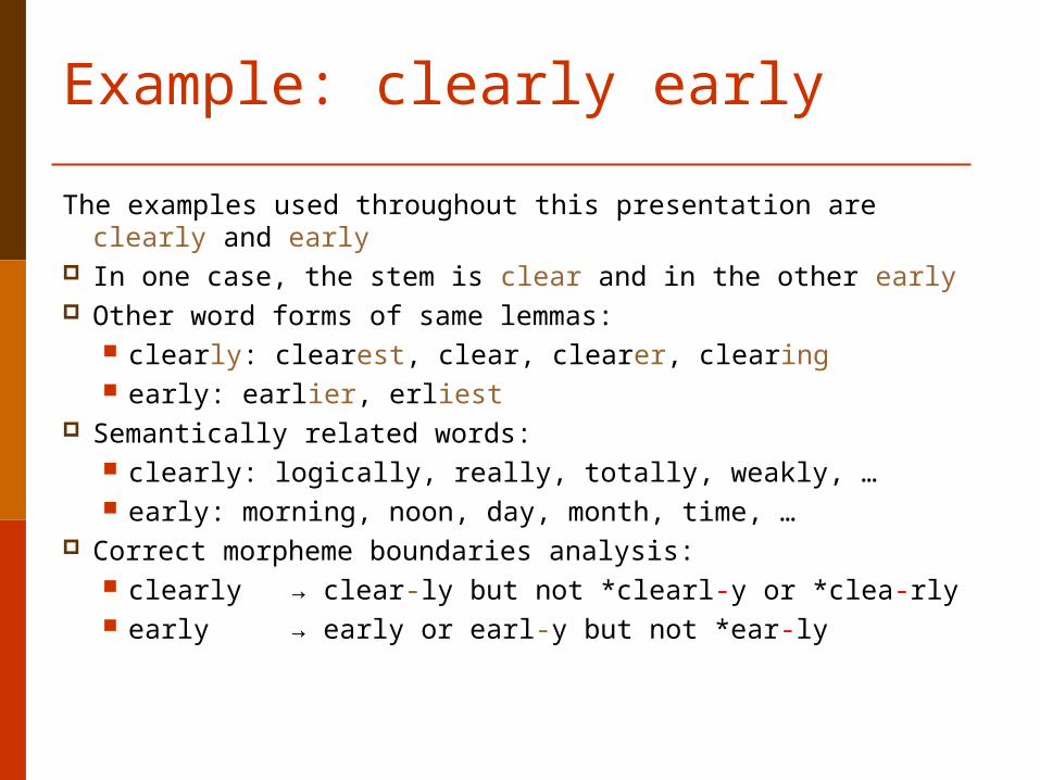
The examples used throughout this presentation are clearly and early
In one case, the stem is clear and in the other early Other word forms of same lemmas:
clearly: clearest, clear, clearer, clearing early: earlier, erliest
Semantically related words: clearly: logically, really, totally, weakly, … early: morning, noon, day, month, time, …
Correct morpheme boundaries analysis: clearly → clear-ly but not *clearl-y or *clea-rly early → early or earl-y but not *ear-ly
Three approaches to morpheme boundary detection
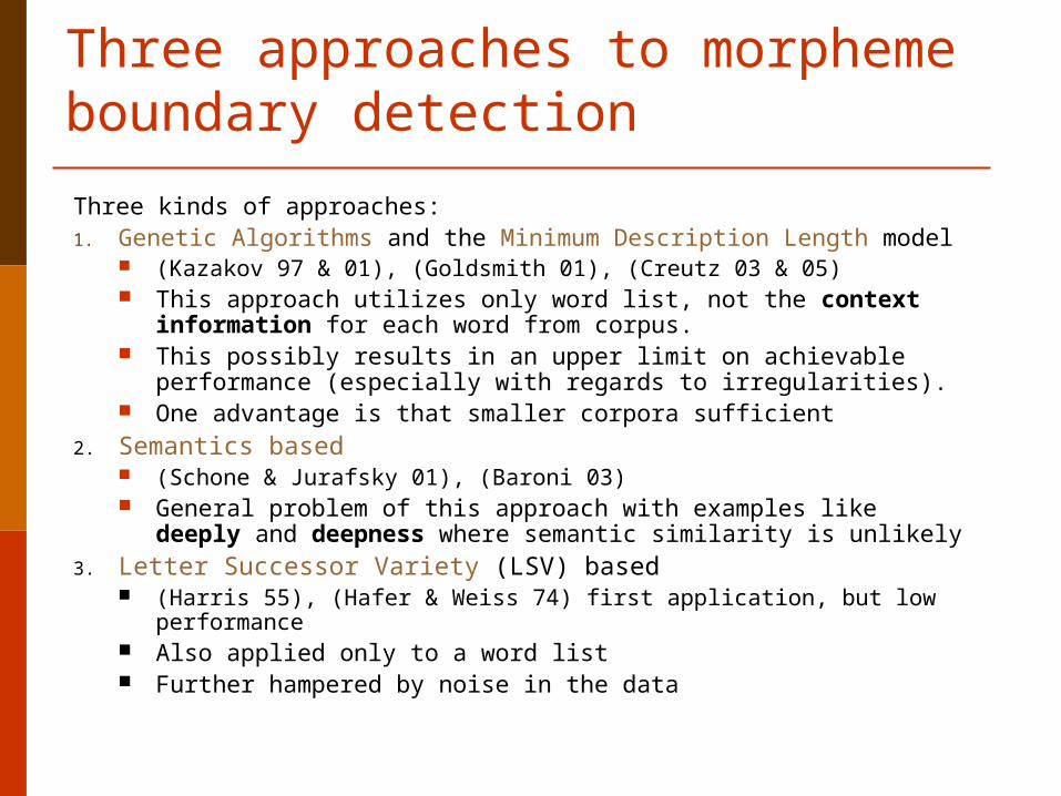
Three kinds of approaches: 1. Genetic Algorithms and the Minimum Description Length model
(Kazakov 97 & 01), (Goldsmith 01), (Creutz 03 & 05) This approach utilizes only word list, not the context information for
each word from corpus. This possibly results in an upper limit on achievable performance
(especially with regards to irregularities). One advantage is that smaller corpora sufficient
2. Semantics based (Schone & Jurafsky 01), (Baroni 03) General problem of this approach with examples like deeply and
deepness where semantic similarity is unlikely3. Letter Successor Variety (LSV) based
(Harris 55), (Hafer & Weiss 74) first application, but low performance Also applied only to a word list Further hampered by noise in the data
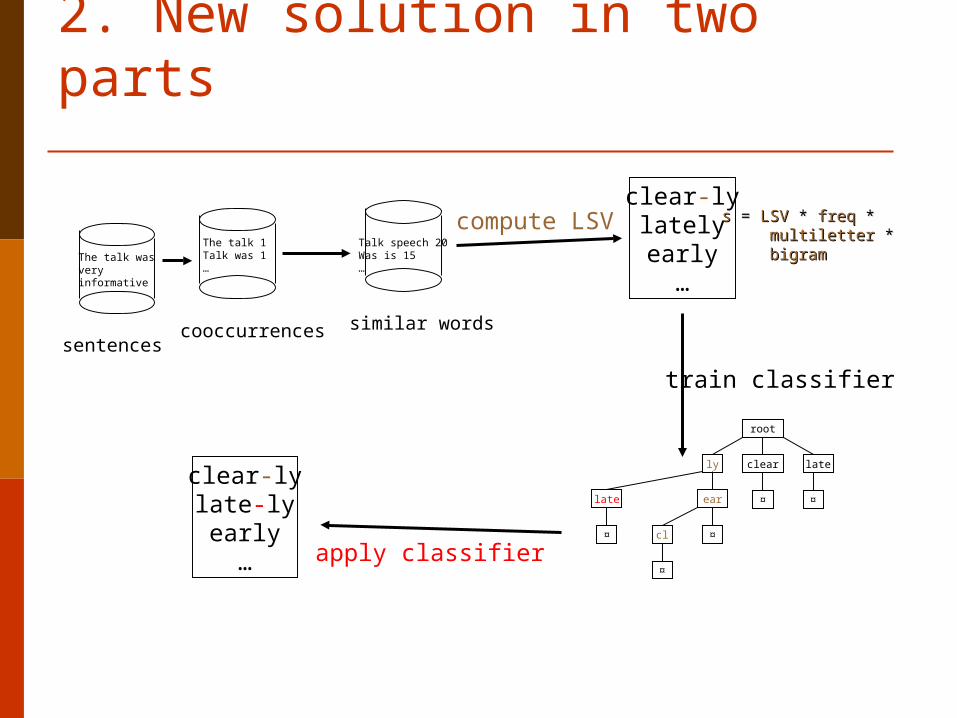
2. New solution in two parts
sentencescooccurrences
The talk wasvery informative
The talk 1Talk was 1…
similar words
Talk speech 20Was is 15…
clear-lylatelyearly
…
clearly late
ear ¤
root
cl
late ¤
¤
¤
¤
train classifier
clear-lylate-lyearly
… apply classifier
compute LSV ss = = LSVLSV * * freqfreq * * multilettermultiletter * * bigrambigram
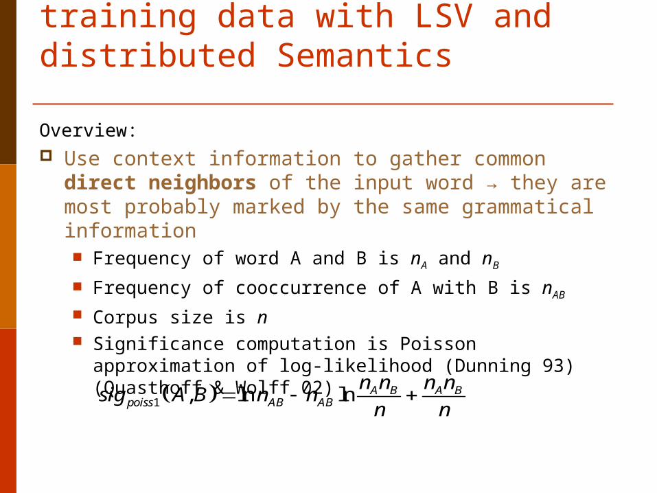
2.1. First part: Generating training data with LSV and distributed Semantics
Overview: Use context information to gather common direct neighbors
of the input word → they are most probably marked by the same grammatical information Frequency of word A and B is nA and nB
Frequency of cooccurrence of A with B is nAB
Corpus size is n Significance computation is Poisson approximation of log-
likelihood (Dunning 93) (Quasthoff & Wolff 02)
1 , ln ln A B A Bpoiss AB AB
n n n nsig A B n n
n n
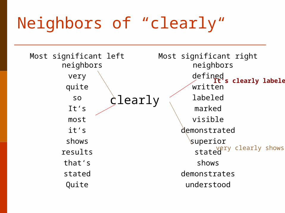
Neighbors of “clearly“
Most significant left neighbors
very
quite
so
It‘s
most
it‘s
shows
results
that‘s
stated
Quite
Most significant right neighbors
defined
written
labeled
marked
visible
demonstrated
superior
stated
shows
demonstrates
understood
clearly
It’s clearly labeled
very clearly shows
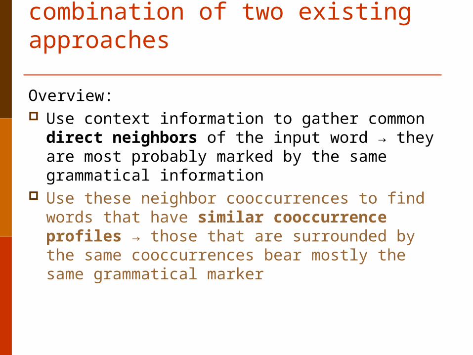
2.2. New solution as combination of two existing approaches
Overview: Use context information to gather common direct
neighbors of the input word → they are most probably marked by the same grammatical information
Use these neighbor cooccurrences to find words that have similar cooccurrence profiles → those that are surrounded by the same cooccurrences bear mostly the same grammatical marker
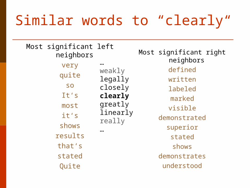
Similar words to “clearly“
Most significant right neighbors
defined
written
labeled
marked
visible
demonstrated
superior
stated
shows
demonstrates
understood
…weaklylegallycloselyclearlygreatlylinearlyreally…
Most significant left neighbors
very
quite
so
It‘s
most
it‘s
shows
results
that‘s
stated
Quite
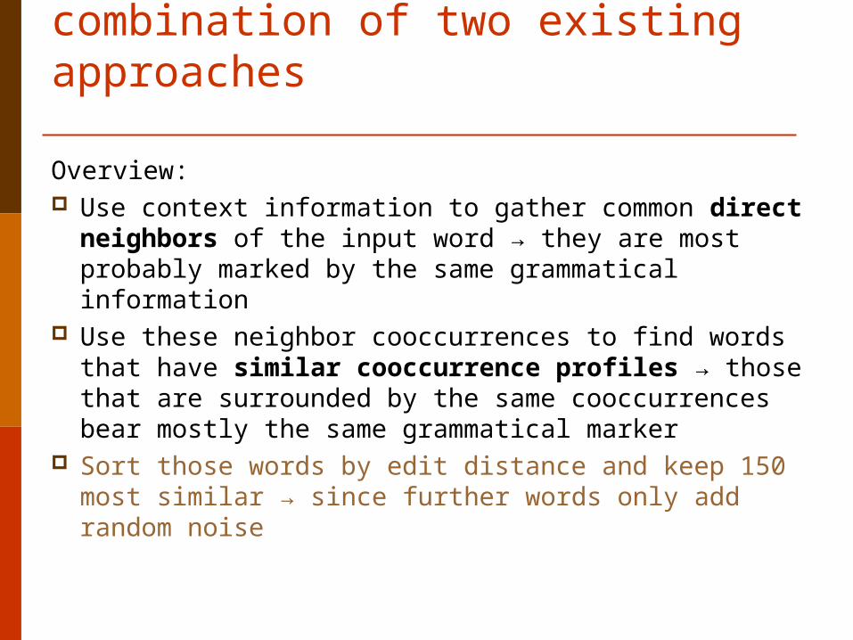
2.3. New solution as combination of two existing approaches
Overview: Use context information to gather common direct
neighbors of the input word → they are most probably marked by the same grammatical information
Use these neighbor cooccurrences to find words that have similar cooccurrence profiles → those that are surrounded by the same cooccurrences bear mostly the same grammatical marker
Sort those words by edit distance and keep 150 most similar → since further words only add random noise
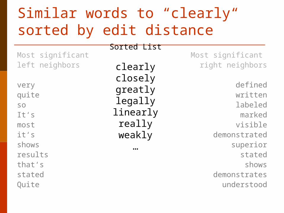
Similar words to “clearly“ sorted by edit distance
Most significant left neighbors
veryquitesoIt‘smostit‘sshowsresultsthat‘sstatedQuite
Most significant right neighbors
definedwritten
labeledmarked
visibledemonstrated
superiorstatedshows
demonstratesunderstood
Sorted List
clearlycloselygreatlylegallylinearlyreally
weakly…
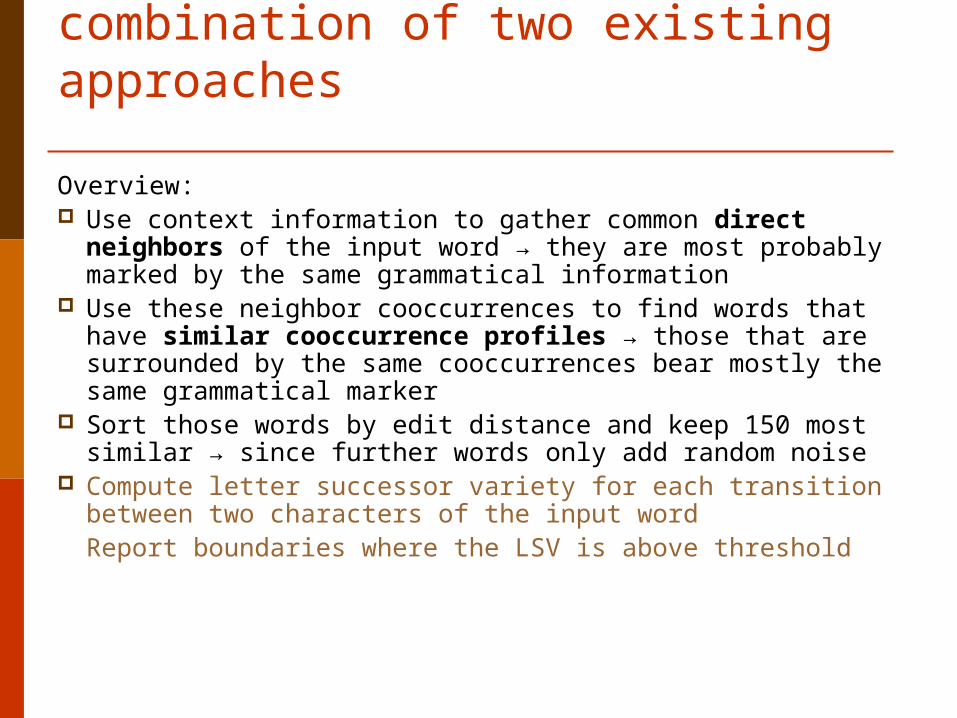
2.4. New solution as combination of two existing approaches
Overview: Use context information to gather common direct
neighbors of the input word → they are most probably marked by the same grammatical information
Use these neighbor cooccurrences to find words that have similar cooccurrence profiles → those that are surrounded by the same cooccurrences bear mostly the same grammatical marker
Sort those words by edit distance and keep 150 most similar → since further words only add random noise
Compute letter successor variety for each transition between two characters of the input wordReport boundaries where the LSV is above threshold
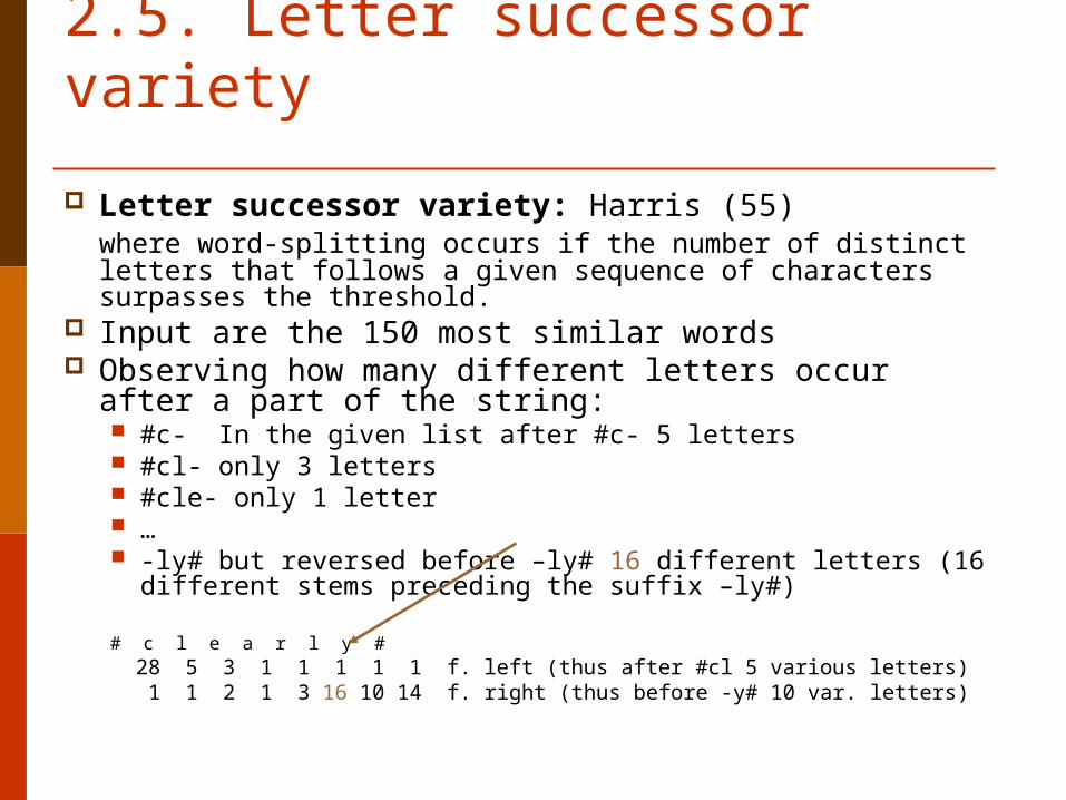
2.5. Letter successor variety
Letter successor variety: Harris (55)where word-splitting occurs if the number of distinct letters that follows a given sequence of characters surpasses the threshold.
Input are the 150 most similar words Observing how many different letters occur after a part of the
string: #c- In the given list after #c- 5 letters #cl- only 3 letters #cle- only 1 letter … -ly# but reversed before –ly# 16 different letters (16 different stems
preceding the suffix –ly#)
# c l e a r l y # 28 5 3 1 1 1 1 1 f. left (thus after #cl 5 various letters) 1 1 2 1 3 16 10 14 f. right (thus before -y# 10 var. letters)
2.5.1. Balancing factors
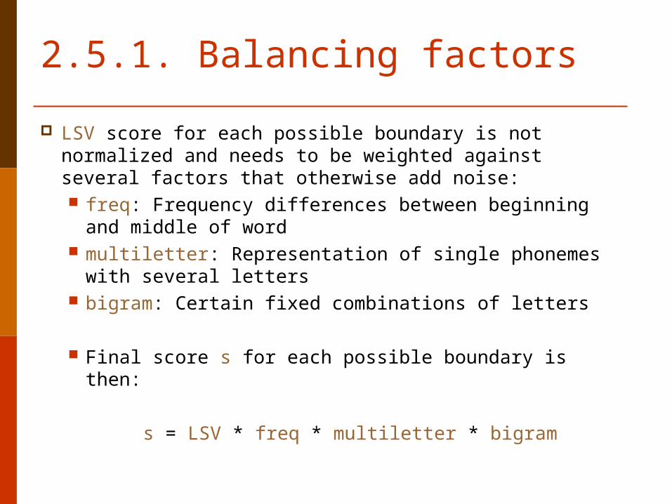
LSV score for each possible boundary is not normalized and needs to be weighted against several factors that otherwise add noise: freq: Frequency differences between beginning and middle
of word multiletter: Representation of single phonemes with
several letters bigram: Certain fixed combinations of letters
Final score s for each possible boundary is then:
s = LSV * freq * multiletter * bigram
2.5.2. Balancing factors: Frequency
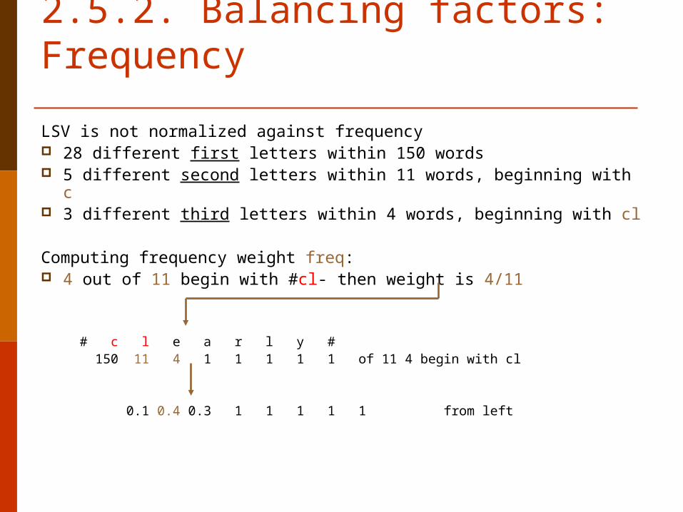
LSV is not normalized against frequency 28 different first letters within 150 words 5 different second letters within 11 words, beginning with c 3 different third letters within 4 words, beginning with cl
Computing frequency weight freq: 4 out of 11 begin with #cl- then weight is 4/11
# c l e a r l y # 150 11 4 1 1 1 1 1 of 11 4 begin with cl 0.1 0.4 0.3 1 1 1 1 1 from left
2.5.3. Balancing factors: Multiletter Phonemes
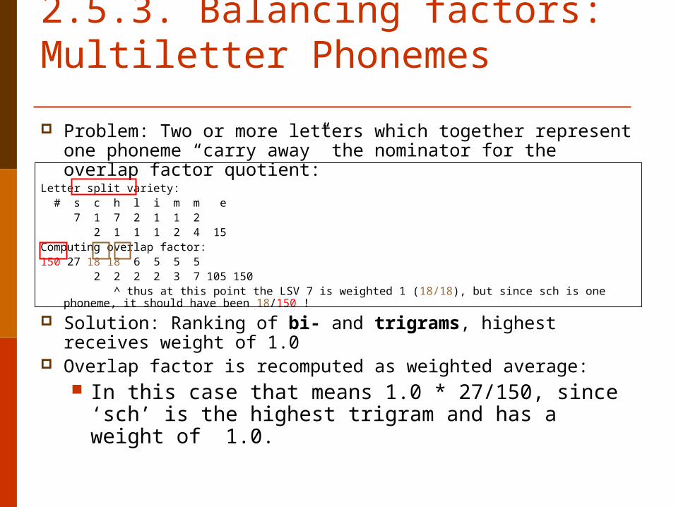
Problem: Two or more letters which together represent one phoneme “carry away” the nominator for the overlap factor quotient:
Letter split variety: # s c h l i m m e 7 1 7 2 1 1 2 2 1 1 1 2 4 15 Computing overlap factor: 150 27 18 18 6 5 5 5 2 2 2 2 3 7 105 150 ^ thus at this point the LSV 7 is weighted 1 (18/18), but since sch is
one phoneme, it should have been 18/150 !
Solution: Ranking of bi- and trigrams, highest receives weight of 1.0
Overlap factor is recomputed as weighted average: In this case that means 1.0 * 27/150, since ‘sch’ is the
highest trigram and has a weight of 1.0.
2.5.4. Balancing factors: Bigrams
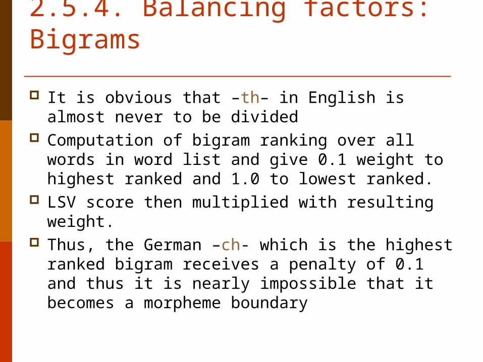
It is obvious that –th– in English is almost never to be divided
Computation of bigram ranking over all words in word list and give 0.1 weight to highest ranked and 1.0 to lowest ranked.
LSV score then multiplied with resulting weight. Thus, the German –ch- which is the highest ranked
bigram receives a penalty of 0.1 and thus it is nearly impossible that it becomes a morpheme boundary
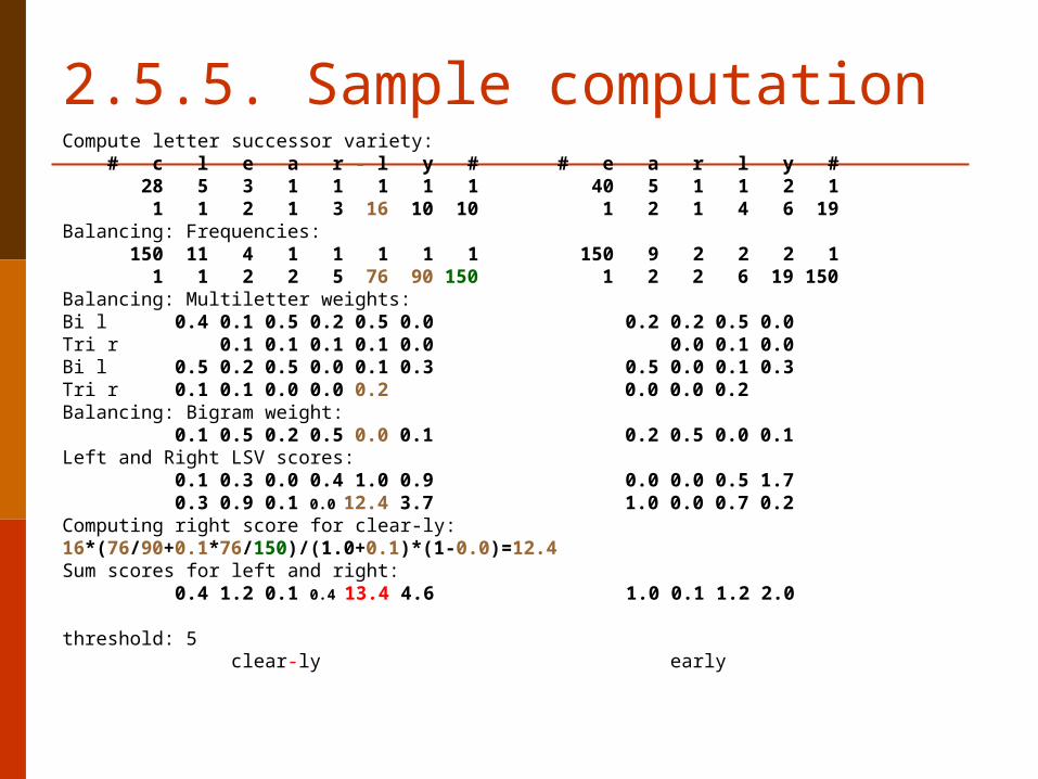
2.5.5. Sample computationCompute letter successor variety: # c l e a r - l y # # e a r l y # 28 5 3 1 1 1 1 1 40 5 1 1 2 1 1 1 2 1 3 16 10 10 1 2 1 4 6 19Balancing: Frequencies: 150 11 4 1 1 1 1 1 150 9 2 2 2 1 1 1 2 2 5 76 90 150 1 2 2 6 19 150Balancing: Multiletter weights:Bi l 0.4 0.1 0.5 0.2 0.5 0.0 0.2 0.2 0.5 0.0Tri r 0.1 0.1 0.1 0.1 0.0 0.0 0.1 0.0Bi l 0.5 0.2 0.5 0.0 0.1 0.3 0.5 0.0 0.1 0.3Tri r 0.1 0.1 0.0 0.0 0.2 0.0 0.0 0.2Balancing: Bigram weight: 0.1 0.5 0.2 0.5 0.0 0.1 0.2 0.5 0.0 0.1Left and Right LSV scores: 0.1 0.3 0.0 0.4 1.0 0.9 0.0 0.0 0.5 1.7 0.3 0.9 0.1 0.0 12.4 3.7 1.0 0.0 0.7 0.2Computing right score for clear-ly: 16*(76/90+0.1*76/150)/(1.0+0.1)*(1-0.0)=12.4 Sum scores for left and right: 0.4 1.2 0.1 0.4 13.4 4.6 1.0 0.1 1.2 2.0
threshold: 5 clear-ly early
Second Part: Training and Applying classifier
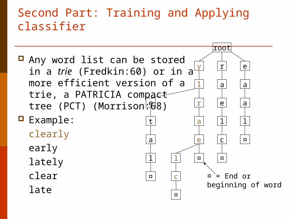
Any word list can be stored in a trie (Fredkin:60) or in a more efficient version of a trie, a PATRICIA compact tree (PCT) (Morrison:68)
Example:
clearly
early
lately
clear
late
ry e
al
t
er a
la l
ce
¤
root
l
c
l
a
e
¤
¤
¤
¤
a
¤ = End or beginning of word
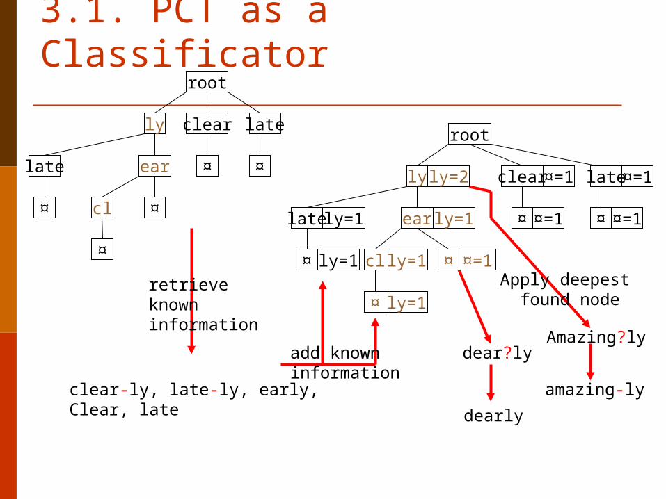
3.1. PCT as a Classificator
clearly late
ear ¤
root
cl
late ¤
¤
¤
¤
clear-ly, late-ly, early,Clear, late
clearly late
ear ¤
root
cl
late ¤
¤
¤
¤
ly=2
ly=1
ly=1
ly=1
Amazing?ly
amazing-ly
ly=1
ly=1
add knowninformation
retrieveknowninformation
Apply deepest found node
dear?ly
dearly
¤=1
¤=1 ¤=1
¤=1¤=1
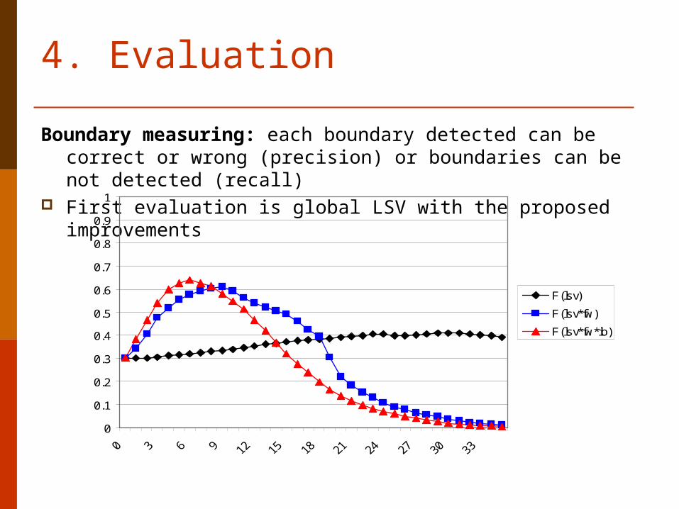
4. Evaluation
Boundary measuring: each boundary detected can be correct or wrong (precision) or boundaries can be not detected (recall)
First evaluation is global LSV with the proposed improvements
0
0.1
0.2
0.3
0.4
0.5
0.6
0.7
0.8
0.9
1
F(lsv)
F(lsv*fw)
F(lsv*fw*ib)
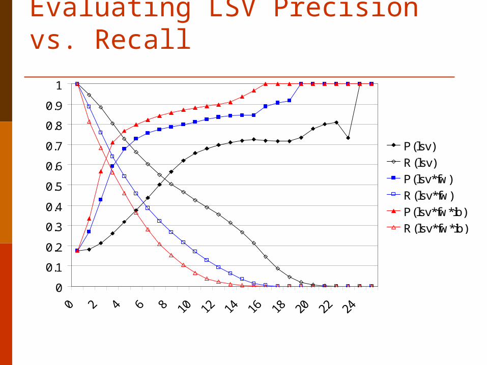
Evaluating LSV Precision vs. Recall
0
0.1
0.2
0.3
0.4
0.5
0.6
0.7
0.8
0.9
1
P(lsv)
R(lsv)
P(lsv*fw)
R(lsv*fw)
P(lsv*fw*ib)
R(lsv*fw*ib)
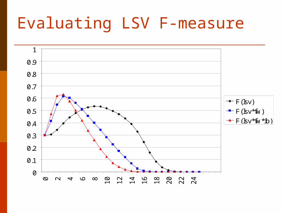
Evaluating LSV F-measure
0
0.1
0.2
0.3
0.4
0.5
0.6
0.7
0.8
0.9
10 2 4 6 8 10
12
14
16
18
20
22
24
F(lsv)
F(lsv*fw)
F(lsv*fw*ib)
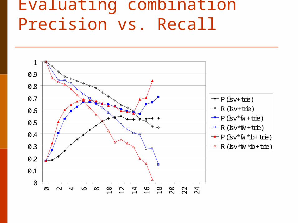
Evaluating combination Precision vs. Recall
0
0.1
0.2
0.3
0.4
0.5
0.6
0.7
0.8
0.9
1
0 2 4 6 8 10
12
14
16
18
20
22
24
P(lsv+trie)
R(lsv+trie)
P(lsv*fw+trie)
R(lsv*fw+trie)
P(lsv*fw*ib+trie)
R(lsv*fw*ib+trie)
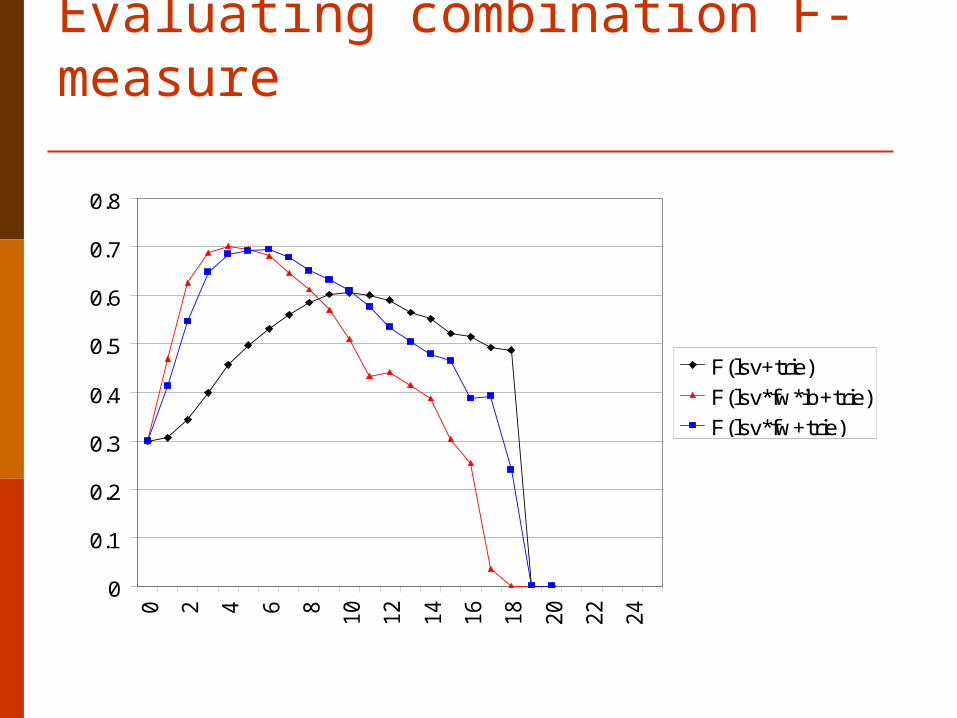
Evaluating combination F-measure
0
0.1
0.2
0.3
0.4
0.5
0.6
0.7
0.8
0 2 4 6 8 10
12
14
16
18
20
22
24
F(lsv+trie)
F(lsv*fw*ib+trie)
F(lsv*fw+trie)
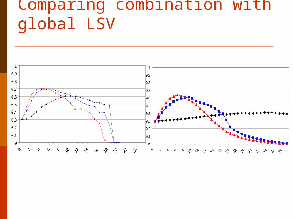
Comparing combination with global LSV
0
0.1
0.2
0.3
0.4
0.5
0.6
0.7
0.8
0.9
1
0
0.1
0.2
0.3
0.4
0.5
0.6
0.7
0.8
0.9
1
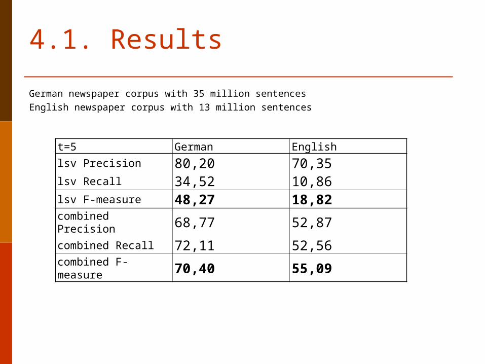
4.1. Results
German newspaper corpus with 35 million sentences
English newspaper corpus with 13 million sentences
t=5 German English
lsv Precision 80,20 70,35lsv Recall 34,52 10,86lsv F-measure 48,27 18,82combined Precision 68,77 52,87combined Recall 72,11 52,56combined F-measure 70,40 55,09
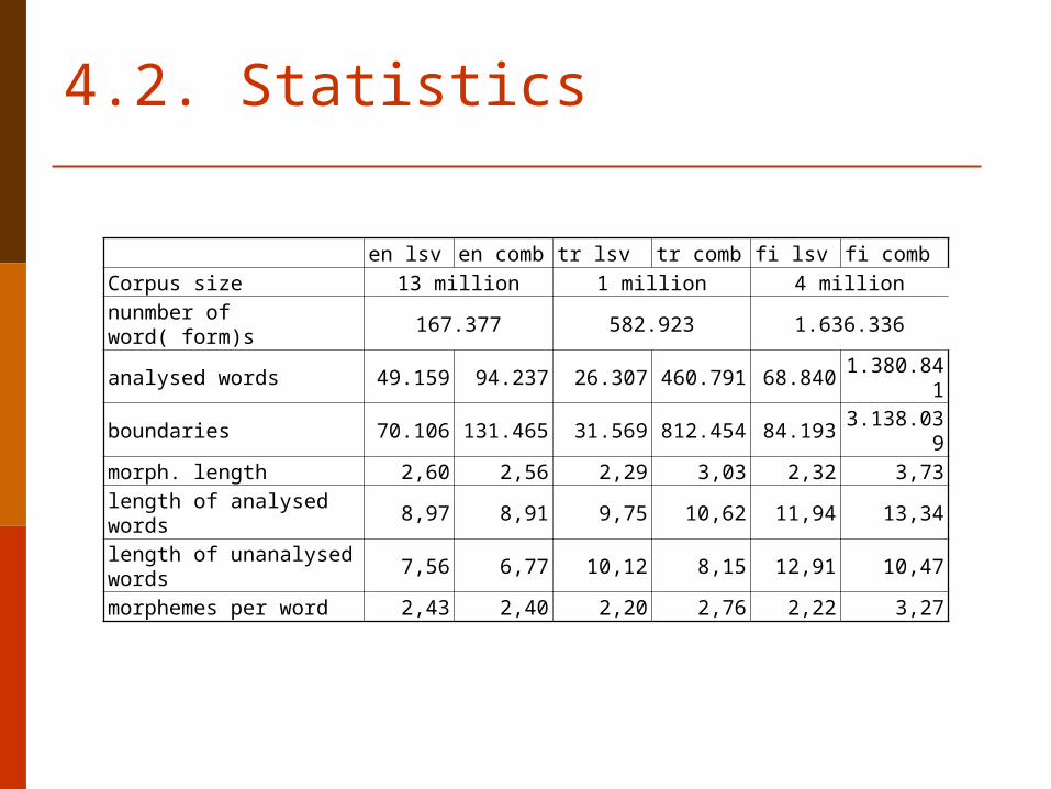
4.2. Statistics
en lsv en comb tr lsv tr comb fi lsv fi comb
Corpus size 13 million 1 million 4 million
nunmber of word( form)s 167.377 582.923 1.636.336
analysed words 49.159 94.237 26.307 460.791 68.840 1.380.841
boundaries 70.106 131.465 31.569 812.454 84.193 3.138.039
morph. length 2,60 2,56 2,29 3,03 2,32 3,73
length of analysed words 8,97 8,91 9,75 10,62 11,94 13,34
length of unanalysed words 7,56 6,77 10,12 8,15 12,91 10,47
morphemes per word 2,43 2,40 2,20 2,76 2,22 3,27
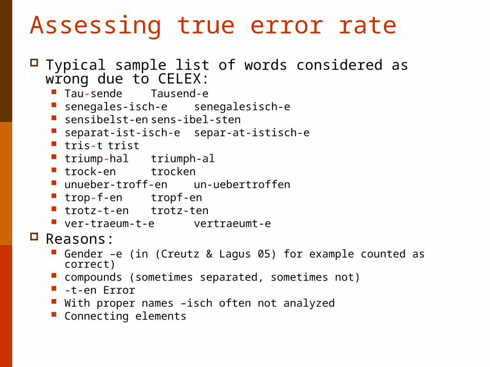
Assessing true error rate Typical sample list of words considered as wrong due to
CELEX: Tau-sende Tausend-e senegales-isch-e senegalesisch-e sensibelst-en sens-ibel-sten separat-ist-isch-e separ-at-istisch-e tris-t trist triump-hal triumph-al trock-en trocken unueber-troff-en un-uebertroffen trop-f-en tropf-en trotz-t-en trotz-ten ver-traeum-t-e vertraeumt-e
Reasons: Gender –e (in (Creutz & Lagus 05) for example counted as correct) compounds (sometimes separated, sometimes not) -t-en Error With proper names –isch often not analyzed Connecting elements
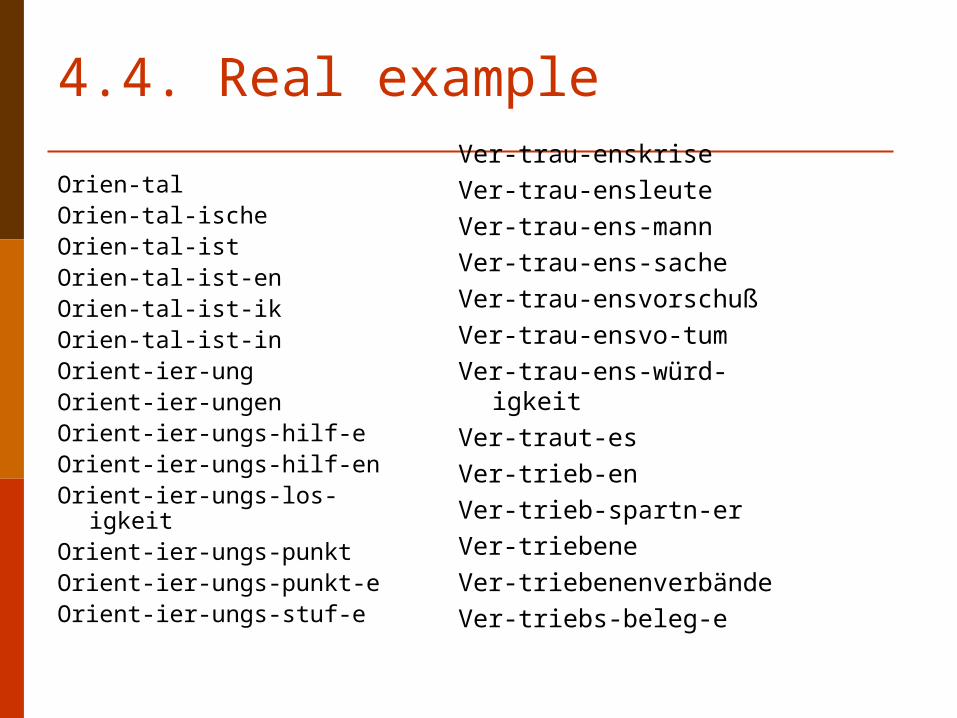
4.4. Real example
Orien-talOrien-tal-ischeOrien-tal-istOrien-tal-ist-enOrien-tal-ist-ikOrien-tal-ist-inOrient-ier-ungOrient-ier-ungenOrient-ier-ungs-hilf-eOrient-ier-ungs-hilf-enOrient-ier-ungs-los-igkeitOrient-ier-ungs-punktOrient-ier-ungs-punkt-eOrient-ier-ungs-stuf-e
Ver-trau-enskrise
Ver-trau-ensleute
Ver-trau-ens-mann
Ver-trau-ens-sache
Ver-trau-ensvorschuß
Ver-trau-ensvo-tum
Ver-trau-ens-würd-igkeit
Ver-traut-es
Ver-trieb-en
Ver-trieb-spartn-er
Ver-triebene
Ver-triebenenverbände
Ver-triebs-beleg-e
5. Further research
Examine quality on various language types Improve trie-based classificator Possibly combine with other existing algorithms Find out how to acquire morphology of non-
concatenative languages Deeper analysis:
find deletions alternations insertions morpheme classes etc.
References
(Argamon et al. 04) Shlomo Argamon, Navot Akiva, Amihood Amir, and Oren Kapah. Effcient unsupervized recursive word segmentation using minimun desctiption length. In Proceedings of Coling 2004, Geneva, Switzerland, 2004. GLDV-Tagung, pages 93-99, Leipzig, March 1998. Deutscher Universitätsverlag.
(Baroni 03) Marco Baroni. Distribution-driven morpheme discovery: A computational/experimental study. Yearbook of Morphology, pages 213-248, 2003. France, http://www.sle.sharp.co.uk/senseval2/, 5-6 July 2001.
(Creutz & Lagus 05) Mathias Creutz and Krista Lagus. Unsupervised morpheme segmentation and morphology induction from text corpora using morfessor 1.0. In Publications in Computer and Information Science, Report A81. Helsinki University of Technology, March 2005.
(Déjean 98) Hervé Déjean. Morphemes as necessary concept for structures discovery from untagged corpora. In D.M.W. Powers, editor, NeMLaP3/CoNLL98 Workshop on Paradigms and Grounding in Natural Language Learning, ACL, pages 295-299, Adelaide, January 1998.
(Dunning 93) T. E. Dunning. Accurate methods for the statistics of surprise and coincidence. Computational Linguistics, 19(1):61-74, 1993.
6. References II
(Goldsmith 01) John Goldsmith. Unsupervised learning of the morphology of a natural language. Computational Linguistics, 27(2):153-198, 2001.
(Hafer & Weiss 74) Margaret A. Hafer and Stephen F. Weiss. Word segmentation by letter successor varieties. Information Storage and Retrieval, 10:371-385, 1974.
(Harris 55) Zellig S. Harris. From phonemes to morphemes. Language, 31(2):190-222, 1955.
(Kazakov 97) Dimitar Kazakov. Unsupervised learning of na¨ive morphology with genetic algorithms. In A. van den Bosch, W. Daelemans, and A. Weijters, editors, Workshop Notes of the ECML/MLnet Workshop on Empirical Learning of Natural Language Processing Tasks, pages 105-112, Prague, Czech Republic, April 1997.
(Quasthoff & Wolff 02) Uwe Quasthoff and Christian Wolff. The poisson collocation measure and its applications. In Second International Workshop on Computational Approaches to Collocations. 2002.
(Schone & Jurafsky 01) Patrick Schone and Daniel Jurafsky. Language-independent induction of part of speech class labels using only language universals. In Workshop at IJCAI-2001, Seattle, WA., August 2001. Machine Learning: Beyond Supervision.
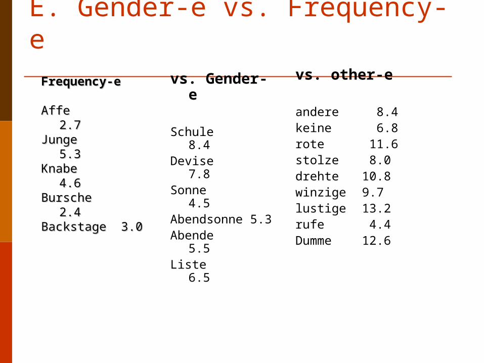
E. Gender-e vs. Frequency-evs. Gender-
e
Schule 8.4Devise 7.8Sonne 4.5Abendsonne 5.3Abende 5.5Liste 6.5
vs. other-e
andere 8.4keine 6.8rote 11.6stolze 8.0drehte 10.8winzige 9.7lustige 13.2rufe 4.4Dumme 12.6
Frequency-eFrequency-e
Affe Affe 2.72.7Junge Junge 5.35.3Knabe Knabe 4.64.6Bursche 2.4Bursche 2.4Backstage 3.0Backstage 3.0