Expert Systems with Applications 38 (2011) 13073–13081

Contents lists available at ScienceDirect

Expert Systems with Applications

journal homepage: www.elsevier .com/locate /eswa

Monthly streamflow forecasting based on improved support vector machine model

Jun Guo, Jianzhong Zhou ⇑, Hui Qin, Qiang Zou, Qingqing LiCollege of Hydropower and Information Engineering, Huazhong University of Science and Technology, Wuhan 430074, China

a r t i c l e i n f o a b s t r a c t

Keywords:Support vector machineStreamflow forecastAdaptive insensitive factorWaveletChaos and phase-space reconstructiontheoryArtificial neural network

0957-4174/$ - see front matter � 2011 Elsevier Ltd. Adoi:10.1016/j.eswa.2011.04.114

⇑ Corresponding author.E-mail addresses: jz.zhou@hust.edu.cn, prof.zhou.h

To improve the performance of the support vector machine (SVM) model in predicting monthly stream-flow, an improved SVM model with adaptive insensitive factor is proposed in this paper. Meanwhile, con-sidering the influence of noise and the disadvantages of traditional noise eliminating technologies, herethe wavelet denoise method is applied to reduce or eliminate the noise in runoff time series. Further-more, in order to avoid the subjective arbitrariness of artificial judgment, the phase-space reconstructiontheory is introduced to determine the structure of the streamflow prediction model. The feasibility of theproposed model is demonstrated through a case study, and the results are compared with the results ofartificial neural network (ANN) model and conventional SVM model. The results verify that the improvedSVM model can process a complex hydrological data series better, and is of better generalization abilityand higher prediction accuracy.

� 2011 Elsevier Ltd. All rights reserved.

1. Introduction

Streamflow forecasting, especially long term forecasting, is ex-tremely important for the optimal management of water re-sources. It has been generally known that streamflow generationprocesses are influenced by both known factors, including precip-itation, evaporation, temperature, etc., and many unknown factors,therefore the streamflow time series always tend to be nonlinear,time-varying and indeterminate, and the under-lying mechanismsof streamflow generation are likely to be quite different duringlow, medium, and high flow periods, especially when extremeevents occur. It is very difficult to make exact prediction of thestreamflow.

A lot of researches on this topic can be found in literatures.Statistics forecast models (Raman & Sunilkumar, 1995; Vapnik,Golowich, & Smola, 1997), such as AR model, MA model, ARIMAmodel, and so on, are used most. Although these models oftenachieve high skill when preforecast conditions are within the rangeof past observations, they can perform poorly in conditions outsideor near the limits of the data (Liu, Zhou, Qiu, Yang, & Liu, 2006). AsANNs have strong ability of nonlinear mapping, they have beensuccessfully applied in a number of diverse fields including waterresources. However, the ANNs do have some drawbacks, such asover-fitting, convergence to local minimum and learning slowly,which make it difficult to gain satisfactory performance when deal-ing with complex hydrological processes. SVM, which is proposedby Cortes and Vapnik (1995), is one of the most effective forecast-ing tools in recent years and considered as an alternative method

ll rights reserved.

ust@263.net (J. Zhou).

of ANNs. SVM is based on the structural risk minimization princi-ple and the VC dimension theory, and basically involves solving aquadratic programming problem, thus can theoretically obtainthe global optimum result of the original problem. In the last dec-ades, the SVM has been applied in the field of hydrology. Xiong andLi (2005) employed the SVM to forecast the Sediment-carryingcapacity; Tripathi, Srinivas, and Nanjundiah (2006) made someresearch on the relationship between climate change and stream-flow using SVM; Lin, Cheng, and Chau (2006) demonstrated theapplication of SVM in predicting monthly river flow discharges inthe Manwan Hydropower Scheme; Yu and Xia (2008) proposed arunoff prediction model based on SVM and chaos theory; Mohsen,Keyvan, Morteza, and Palhang (2009) discussed the performance ofSVM and ANN in runoff modeling, and presented that the SVM isbetter than ANN in some case.

Based on the above research, the SVM model is employed toforecast the streamflow in this research. And the adaptive insensi-tive factor is introduced into SVM to improve the performance ofthe SVM in predicting the monthly streamflow. At the same time,in order to obtain the optimal parameters of the improved SVMmodel, an improved particle swarm optimization (PSO) algorithmis adopted (Behnamian & Ghomi, 2010; Chen & Lin, 2009; He, Zhou,Li, Yang, & Li, 2008; He, Zhou, Xiang, Chen, & Qin, 2009; Lin, Ying,Chen, & Lee, 2008). Besides, different with the recent research ofapplication of SVM in streamflow forecasting (Lin et al., 2006;Mohsen et al., 2009; Yu & Xia, 2008), the PSO optimal algorithm,wavelet denoising method and phase-space reconstruction theoryare all together applied to utilize their specific advantages in thisresearch.

The remainder of this paper is organized as follows: Section 2provides a brief introduction to the methodology mentioned above,

13074 J. Guo et al. / Expert Systems with Applications 38 (2011) 13073–13081

including wavelet denoise method, the chaos theory and thephase-space reconstruction theory, SVM for regression andimproved SVM, PSO algorithm and its improvement, Section 3 pro-vides details of the applying this method in the Three Gorges re-gion as a case study, Section 4 presents and discusses the resultsof the case study, while conclusions are made for this research inSection 5.

2. Brief introduction of methods adopted in this research

Based on the basic modeling theory and method of SVM, an im-proved SVM model with adaptive insensitive factor is proposed inthis paper. Moreover, to further improve the proposed SVM modelperformance in predicting monthly streamflow time series, thewavelet denoising method, parse-space reconstruction methodand PSO algorithm are all together introduced.

Before starting training the SVM model, it is necessary to reduceor eliminate the noise among the sample time series, as streamflowtime series usually involves some noise, which can make greatinfluence on the streamflow forecasting accuracy (Ding & Deng,1988). Due to the complexity and stochastic of the streamflow pro-cesses, conventional denoise methods always have some limita-tions. Fortunately, the wavelet decomposition and reconstructiontheory provide us a effective denoise method. The wavelet is apowerful tool for analyzing and processing time series signal. Thewavelet transform is evolved from Fourier analysis and consideredas a mathematical theory which specifically permits the discrimi-nation of nonstationary signals with different frequency features.It can provide time and frequency information simultaneously.

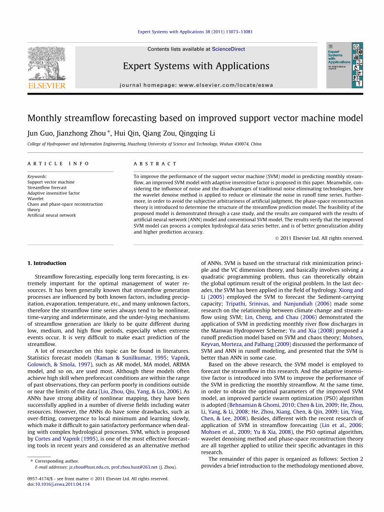
Measured strtime seri

Data denoWavelet denoising method

Determinestructure ofpredicting m

Predicting mconstructImproved SVM model

Model paraoptimizat

Forecaststreamfl

Fig. 1. The topological relation of th

Realizing these advantages in representing the property of time–frequency domain localization, a denoise method base on waveletis adopted in this content. Additionally, recent researches haveshown that there is chaos phenomenon among the hydrology sys-tem (Jayawarderm & Lai, 1994; Sivakumar, 2004), hence the chaostheory and the phase-space reconstruction theory are also intro-duced to analyze the chaos mechanism of the streamflow time ser-ies, it can overcome the disadvantage of arbitrariness of the modelstructure determination as well.

The relationship of the adopted theory or methods is summa-rized as in Fig. 1. And the details are shown as the follow of thissection.

2.1. Wavelet denoise method

Wavelet analysis is multi-resolution analysis in time and fre-quency domain. The wavelet transform decomposes time seriessignals into different resolutions by controlling scaling and shift-ing. It provides a good localization properties obtained in both timeand frequency domains.

If w(t) is a mother wavelet, the wavelet basis function can bederived from the forum (1) as follow:

wa;bðtÞ ¼1ffiffiffiffiffiffijaj

p wt � b

a

� �ða; b 2 R; a – 0Þ ð1Þ

where wa,b(t) is the successive wavelet, a is the scaling factor, b isthe offset factor, and the R represents the real number domain.

For any time series f(t) e L2(R), the successive wavelet transformof f(t) is defined as:

eamflow es

ising

the the odel

Chaotic characteristic analysis and parse-

space reconstruction

odel ion

metersion Improved PSO algorithm

ing ow

e adopted methods or theory.

J. Guo et al. / Expert Systems with Applications 38 (2011) 13073–13081 13075

Wf ða; bÞ ¼1ffiffiffiap

Z þ1

�1f ðtÞw t � b

a

� �dt ð2Þ

where wðtÞ is the complex conjugate functions of w(t). It can be seenfrom Eq. (2) that the wavelet transform is the decomposition of f(t)under different resolution level.

With the successive wavelet transform Wf(a, b), the originaltime series f(t) can be obtained through the wavelet reconstruc-tion, which is defined as:

f ðtÞ ¼Z þ1

�1

jwðxÞj2

jxj dx

!�1 Z þ1

�1

Z þ1

�1

1a2 Wf ða; bÞwa;bðtÞdadb

ð3Þ

where wðxÞ is the Fourier transform of w(t).The noise among the streamflow time series is always signals

with high frequency. Hence, the essence of the wavelet denoisingis to extract the high frequency parts from the signal. The detailsof the wavelet denoise procedure are as follows, including waveletdecomposition, threshold processing and wavelet reconstruction:

Step 1: Wavelet decomposition. Select a proper wavelet func-tion and determine a suitable decomposition level N. Then cal-culate the wavelet transform of the original time series usingEq. (2). After that, we can acquire one low-frequency waveletcoefficients series and N high-frequency wavelet coefficientsseries.Step 2: Threshold processing. In general, a threshold T is used todetermine whether high-frequency wavelet coefficients to beinsignificant in wavelet transform coding of signals. It is properto set different thresholds to different layers. The threshold T iscalculated by unbiased likelihood estimation method in thisapproach.Step 3: Wavelet reconstruction. With the low-frequency wave-let coefficients series calculated from the step 1 and N high-fre-quency wavelet coefficients series after threshold processing,the denoised time series can be obtain through wavelet recon-struction using Eq. (3).

2.2. Phase-space reconstruction

As the streamflow time series is single-dimensional series, themethod used in this paper takes the concept of reconstruction ofa single-variable series (using its past history and a method of de-lays) into a multi-dimensional phase space to represent the under-lying dynamics. For some streamflow time series Xt, wherei = 1, 2, . . . , N, the phase space can be reconstructed according to:

Yj ¼ ðXj;Xjþs;Xjþ2s; . . . ;Xjþðm�1ÞsÞ ð4Þ

where j ¼ 1;2; . . . ;N � ðm� 1Þs, m is the embedding dimension, s isthe delay time (Packard, Crutchfield, Farmer, & Shaw, 1980; Takens,1981).

2.2.1. Calculate the delay time sThere are many tools to calculate the value of delay time s, such

as autocorrelation function method, mutual information method,C–C method, etc. In this approach, autocorrelation function meth-od, which is more popular and mature, is adopted (Nu, Lu, & Chen,2002). For chaos time series x1; x2; . . . ; xN , the autocorrelation func-tion of it is defined as:

RðsÞ ¼ 1N

XN�1

i¼0

xixiþs ð5Þ

Then, the figure of R(s) versus s can be plotted. And the value of s,with which R(s) firstly go across the s axis, is the best delays time.

2.2.2. Calculate the best embedding dimension mAlso there are some methods to determine the best embedding

dimension, such as false neighbors method, Cao method, saturatedcorrelation dimension method, and so on. The Cao method is em-ployed to figure out the best embedding dimension in this re-search, and the result is verified by the saturated correlationdimension method.

(1) Cao method:

The Cao method is developed based on the false neighborsmethod, and it keeps some advantages of the false neighbors meth-od. The details about the Cao method can refer to Cao (1997).

(2) Saturated correlation dimension method:

The value of the correlation dimension is calculated accordingto:

CðrÞ ¼ 1

½n� ðm� 1Þs�2Xn�ðm�1Þs

i;j¼1

hðr � jjXðiÞ � XðjÞjjÞ ð6Þ

D ¼ limr!0

log CðrÞlog r

ð7Þ

where r is the critical distance, h(�) represents the Heavisidefunction.

With the increasing of embedding dimension, the correlationdimension of chaos time series will tend to be saturated while thatof stochastic series will increase constantly. It is the characteristicof chaos time series.

2.2.3. Maximum Lyapunov exponentIt is accepted that if the maximum Lyapunov exponent of time

series LE > 0, the time series can be considered as chaos time series.There are several ways of calculating the LE, including Jacobianmethod, Wolf method, small data sets method, and so on. The LE

of the given time series is calculated by means of small data setshere. The theory about the small data sets can be obtain from theRef. Ramsey and Yuan (1990).

2.3. Improved SVM for regression

Similar with ANN, SVM is a data training/fitting technique. Theessence of SVM is to transfer the original problem into solving aquadratic programming problem, it can theoretically obtain theglobal optimum result of the problem, while the ANN is easy toconverge to local minimum. Besides, the computing rate of SVMis significant faster than ANN.

2.3.1. Overview of basic SVM for regressionSuppose the sample data for training is {Xi, yi}, where

i = 1, 2, . . . , l, Xi is the input, and yi is the output. The aim of SVMfor regression is to find a function of this form:

yi ¼W � Xi þ b ð8Þ

where W is a hyperplane, and b is the offset.The regression SVM will use a penalty function as:

jyi � ðW � Xi þ bÞj 6 e; not allocating a penaltyjyi � ðW � Xi þ bÞj > e; allocating a penalty

�ð9Þ

Referring to Fig. 2, the region bound by yi ± e is called an e-insen-sitive tube. And the goal of this problem can be written accordingto:

Fig. 2. SVM for regression with e-insensitive tube.

13076 J. Guo et al. / Expert Systems with Applications 38 (2011) 13073–13081

min12jjWjj2 þ C

Xl

i¼1

LeðXi; yi; f Þ" #

ð10Þ

where the Le(Xi, yi, f) is defined as:

LeðXi; yi; f Þ ¼maxð0; jf ðXiÞ � yij � eÞ ð11Þ

And as the existence of fitting errors, the slack variables n+ andn- are introduced, then the model form of SVM for regression willbe as:

min12kWk2 þ C

Xl

i¼1

ðnþi þ xi�i Þ" #

ð12Þ

Subject to : ðW � Xi þ bÞ � yi 6 eþ nþ

yi � ðW � Xi þ bÞ 6 eþ n�

nþ > 0; n� > 0i ¼ 1;2; . . . ; l

The corresponding dual problem can be derived using the now stan-dard techniques:

maxXl

i¼1

aþi � a�i� �

yi � eXl

i¼1

aþi þ a�i� �"

�12

Xi;j

aþi � a�i� �

aþj � a�j�

Xi � Xj

#ð13Þ

Subject to : 0 6 aþi 6 C;0 6 a�i 6 C

Xl

i¼1

ðaþi � a�i Þ ¼ 0

i ¼ 1;2; . . . ; l

Solve this problem with quadratic programming method, then wecan acquire the regression function of the system. However, fromthe above explanation, it can be noted that it is not suitable for non-linear system, especially for the complex and high nonlinearstreamflow time series. Fortunately, the Kernel function can helpus to leap this obstacle, as it can map the lower dimension data intoa higher dimension linear space defined implicitly by nonlinear ker-nel function. When Kernel function is introduced, the goal functionof the above problem will be explained according to:

max½Xl

i¼1

aþi � a�i� �

yi � eXl

i¼1

aþi þ a�i� �

� 12

Xi;j

aþi � a�i� �

aþj � a�j�

KðXi;XjÞ� ð14Þ

where the K(Xi, Xj) is the Kernel Trick, e.g. if the kernel function isRadial Basis Kernel, then KðXi;XjÞ ¼ expð� kXi�Xjk2

2r2 Þ.

2.3.2. Improved SVM for regressionIt is known that there are a lot of criterions for accessing the

forecasting quality, such as mean absolute error (MAE), mean rel-ative error (MRE), determination coefficient (R2), maximum abso-lute error, maximum relative error, and so on. But in practice, thequalified rate, which is defined as the proportion of the predictedvalues with relative error below 20%, is used most. Suppose themeasured runoff time series is {y1, y2, . . . , yn}, and the predictedrunoff value is fy01; y02; . . . ; y0ng, then the qualified rate can be calcu-lated according to:

Rq ¼1n

Xn

i¼1

ti ð15Þ

where ti ¼1;

jyi�y0ij

yi� 100% 6 20%

0; jyi�y0ij

yi� 100% > 20%

8<: ; ði ¼ 1;2; . . . ;nÞ

In other words, the tolerance of the predicted error is 0.2yi,which is variable versus the actual value yi. Hence, during thetraining term of the SVM for regression, it is appropriate to changethe constant insensitive factor e into an adaptive variable insensi-tive factor, which is defined as a function of output of the modele(yi) in this approach. Therefore, the goal function of the dual prob-lem will be expressed as:

maxXl

i¼1

aþi � a�i� �

yi � eðyiÞXl

i¼1

aþi þ a�i� �"

�12

Xi;j

aþi � a�i� �

aþj � a�j�

KðXi;XjÞ#

Two typical functions e(yi),which are shown below, are discussed inthe case study. One is a linear function of yi, and the other isnonlinear.

e1ðyiÞ ¼ a1yi þ a2 ð16Þ

e2ðyiÞ ¼ b1eb2yi þ b3 ð17Þ

The improved SVM with a linear adaptive insensitive factor is calledLAIF-SVM, while the improved SVM with a nonlinear adaptiveinsensitive factor is called NAIF-SVM in this paper. The results ofthe case study, which is explained in Section 3, show that the adap-tive insensitive factor e(yi) can enhance the generalization ability ofSVM, and the predicted accuracy is also improved in some way.

2.4. PSO algorithm

PSO algorithm was first introduced in 1995 by social-psycholo-gist Eberhart and electrical engineer Kennedy and Eberhart (1995).It is a swarm intelligence inspired by the behavior of bird flocks.Due to its high convergence speed and easy to realize, it has beenwidely employed to solve variable optimization problems (Feng,Chen, & Ye, 2007; Huang, Huang, & Cheng, 2008; Vlachogiannis &Lee, 2009; Zhao & Yang, 2009).

2.4.1. Basic PSO algorithmSuppose in a D-dimension search space, the number of the par-

ticles is N, the particle swarm is {Xi|i = 1, 2, . . . , N}, whereXi = {xij|j = 1, 2, . . . , D}, and each particle has a velocityVi = {vij|j = 1, 2, . . . , D}. Each particle updates its position Xi andvelocity Vi in every iteration by the following two formulas:

vgþ1ij ¼ w�vg

ij þ c1 � randðÞ�ðPbestgij � xg

ijÞ þ c2 � randðÞ�ðGbestgj � xg

ijÞð18Þ

xgþ1ij ¼ xg

ij þ vgþ1ij ð19Þ

0 200 400 600 800 1000 1200-60

-40

-20

0

20

40

60

Time / month

Flow

/ m

3 /s

Fig. 4. The noise exist in the measured streamflow time series.

J. Guo et al. / Expert Systems with Applications 38 (2011) 13073–13081 13077

where i = 1, 2, . . . , N; j = 1, 2, . . . , D, w is inertia factor, c1 and c2 areacceleration coefficients, Pbestg

ij represents the best position of jthdimension of ith particle itself encountered by the gth iteration,and Gbestg

j denotes the best position of jth dimension of the wholeswarm encountered by the gth iteration.

2.4.2. Improved PSO algorithmResearch has revealed that a larger inertia weight facilitates glo-

bal exploration and a smaller inertia weight tends to facilitate localexploration to fine-tune the current search area (Liu, Wang, Jin,Tang, & Huang, 2005). In this study, the inertia w is set to linearlychange according to the iteration from 0.9 to 0.4 as:

w ¼ 0:9� 0:9� 0:4gmax

� g ð20Þ

where the gmax denotes the preset maximum of iteration number.Although the PSO algorithm has high convergence speed, it

could easily be premature convergence and fall into localminimum. To overcome this problem, the mutation operation isintroduced as:

xgij ¼

minðmaxðxgij þ c � randðÞ; xmin

j Þ; xmaxj Þ; if randðÞ > pm

xgij; if randðÞ 6 pm

(

ð21Þ

where xminj ; xmax

j are minimum and maximum value of the j-dimen-sion respectively, c is a constant real number, which has the value of0.5 in this approach, and pm is the preset probability of mutation.

3. Case study

3.1. Introduction of the study area

The Changjiang (Yangtze) River basin, as shown in Fig. 3, is se-lected in this research. The Changjiang River originates in the Qing-hai-Tibet Plateau and flows about 6300 km eastwards to the EastChina Sea. The drainage basin lies between 91�E–122�E and25�N–35�N, covering a total area of 1808.5 � 103 km2. With thecompletion of the Three Gorges Hydropower plant, which is thelargest hydropower plant of the world, the Yangtze River hydro-power resources will be effectively developed and utilized. As theThree Gorges Dam has interests in control of flooding, hydroelec-tric power generation agriculture, and municipal and industrialwater supply, the streamflow forecast, especially the long-termstreamflow forecast, is significant to the optimal operation of theThree Gorges Dam. The precisely streamflow forecasting, especially

Fig. 3. The Changjia

long term streamflow forecasting, can make considerable eco-nomic benefit as well as be good for flood controlling downstreamof the Yangtze River.

3.2. Monthly streamflow forecasting

The monthly streamflow data measured between 1890 and1990 of the Yichang station is chosen in this research. And thestreamflow forecasting procedures are summarized as follows:

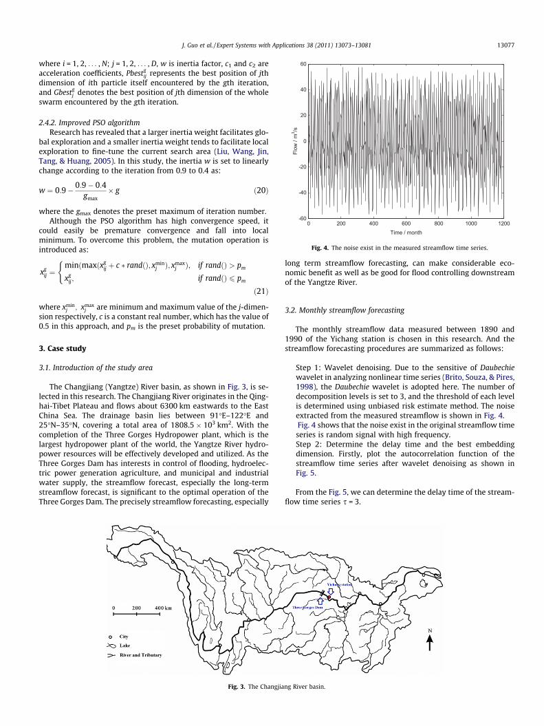
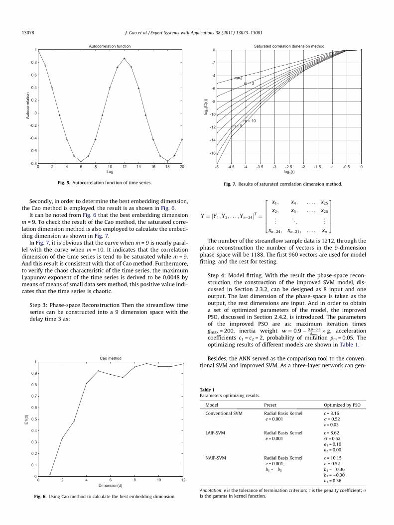
Step 1: Wavelet denoising. Due to the sensitive of Daubechiewavelet in analyzing nonlinear time series (Brito, Souza, & Pires,1998), the Daubechie wavelet is adopted here. The number ofdecomposition levels is set to 3, and the threshold of each levelis determined using unbiased risk estimate method. The noiseextracted from the measured streamflow is shown in Fig. 4.Fig. 4 shows that the noise exist in the original streamflow timeseries is random signal with high frequency.Step 2: Determine the delay time and the best embeddingdimension. Firstly, plot the autocorrelation function of thestreamflow time series after wavelet denoising as shown inFig. 5.

From the Fig. 5, we can determine the delay time of the stream-flow time series s = 3.

ng River basin.

0 2 4 6 8 10 12 14 16 18 20-0.8

-0.6

-0.4

-0.2

0

0.2

0.4

0.6

0.8

1

Lag

Auto

corre

latio

n

Autocorrelation function

Fig. 5. Autocorrelation function of time series.

-5 -4.5 -4 -3.5 -3 -2.5 -2 -1.5 -1 -0.5 0

-16

-14

-12

-10

-8

-6

-4

-2

0

log2(r)

log 2(

C(r)

)

Saturated correlation dimension method

m=2m = 3

m = 9m = 10

Fig. 7. Results of saturated correlation dimension method.

13078 J. Guo et al. / Expert Systems with Applications 38 (2011) 13073–13081

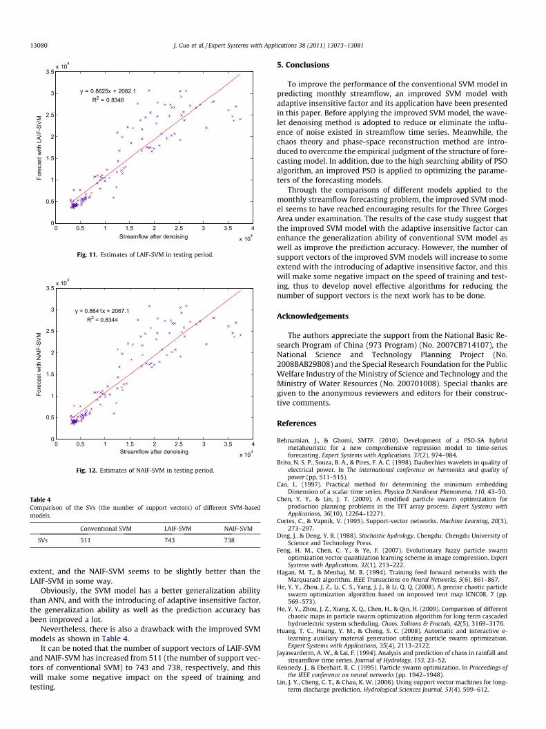
Secondly, in order to determine the best embedding dimension,the Cao method is employed, the result is as shown in Fig. 6.

It can be noted from Fig. 6 that the best embedding dimensionm = 9. To check the result of the Cao method, the saturated corre-lation dimension method is also employed to calculate the embed-ding dimension as shown in Fig. 7.

In Fig. 7, it is obvious that the curve when m = 9 is nearly paral-lel with the curve when m = 10. It indicates that the correlationdimension of the time series is tend to be saturated while m = 9.And this result is consistent with that of Cao method. Furthermore,to verify the chaos characteristic of the time series, the maximumLyapunov exponent of the time series is derived to be 0.0048 bymeans of means of small data sets method, this positive value indi-cates that the time series is chaotic.

Step 3: Phase-space Reconstruction Then the streamflow timeseries can be constructed into a 9 dimension space with thedelay time 3 as:

0 2 4 6 8 10 120

0.1

0.2

0.3

0.4

0.5

0.6

0.7

0.8

0.9

1

Dimension(d)

E1(d

)

Cao method

Fig. 6. Using Cao method to calculate the best embedding dimension.

Y ¼ ½Y1;Y2; . . . ;Yn�24�T ¼

x1; x4; . . . ; x25

x2; x5; . . . ; x26

..

. . .. ..

.

xn�24; xn�21; . . . ; xn

266664

377775

The number of the streamflow sample data is 1212, through thephase reconstruction the number of vectors in the 9-dimensionphase-space will be 1188. The first 960 vectors are used for modelfitting, and the rest for testing.

Step 4: Model fitting. With the result the phase-space recon-struction, the construction of the improved SVM model, dis-cussed in Section 2.3.2, can be designed as 8 input and oneoutput. The last dimension of the phase-space is taken as theoutput, the rest dimensions are input. And in order to obtaina set of optimized parameters of the model, the improvedPSO, discussed in Section 2.4.2, is introduced. The parametersof the improved PSO are as: maximum iteration timesgmax = 200, inertia weight w ¼ 0:9� 0:9�0:4

gmax� g, acceleration

coefficients c1 = c2 = 2, probability of mutation pm = 0.05. Theoptimizing results of different models are shown in Table 1.

Besides, the ANN served as the comparison tool to the conven-tional SVM and improved SVM. As a three-layer network can gen-

Table 1Parameters optimizing results.

Model Preset Optimized by PSO

Conventional SVM Radial Basis Kernele = 0.001

c = 3.16r = 0.52e = 0.03

LAIF-SVM Radial Basis Kernele = 0.001

c = 8.62r = 0.52a1 = 0.10a2 = 0.00

NAIF-SVM Radial Basis Kernele = 0.001;b1 = �b3

c = 10.15r = 0.52b1 = �0.36b2 = �0.30b3 = 0.36

Annotation: e is the tolerance of termination criterion; c is the penalty coefficient; ris the gamma in kernel function.

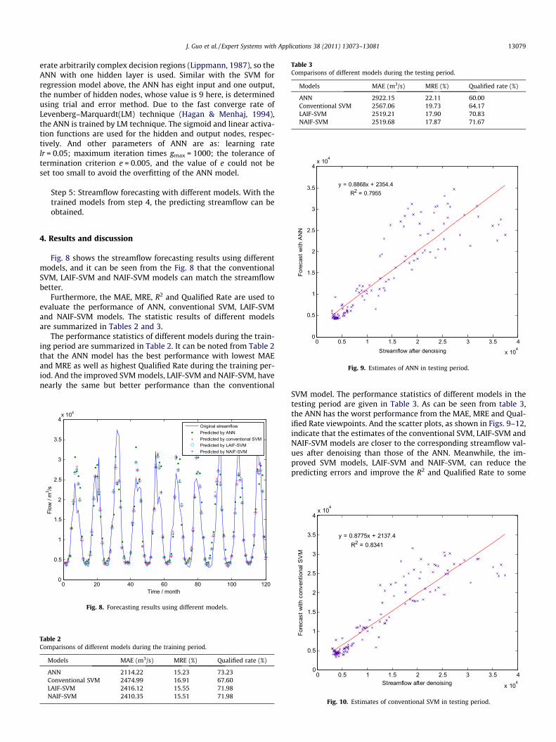
Table 3Comparisons of different models during the testing period.

Models MAE (m3/s) MRE (%) Qualified rate (%)

ANN 2922.15 22.11 60.00Conventional SVM 2567.06 19.73 64.17LAIF-SVM 2519.21 17.90 70.83NAIF-SVM 2519.68 17.87 71.67

0 0.5 1 1.5 2 2.5 3 3.5 4

x 104

0

0.5

1

1.5

2

2.5

3

3.5

4x 104

Fore

cast

with

AN

N

Streamflow after denoising

y = 0.8868x + 2354.4R2 = 0.7955

Fig. 9. Estimates of ANN in testing period.

J. Guo et al. / Expert Systems with Applications 38 (2011) 13073–13081 13079

erate arbitrarily complex decision regions (Lippmann, 1987), so theANN with one hidden layer is used. Similar with the SVM forregression model above, the ANN has eight input and one output,the number of hidden nodes, whose value is 9 here, is determinedusing trial and error method. Due to the fast converge rate ofLevenberg–Marquardt(LM) technique (Hagan & Menhaj, 1994),the ANN is trained by LM technique. The sigmoid and linear activa-tion functions are used for the hidden and output nodes, respec-tively. And other parameters of ANN are as: learning ratelr = 0.05; maximum iteration times gmax = 1000; the tolerance oftermination criterion e = 0.005, and the value of e could not beset too small to avoid the overfitting of the ANN model.

Step 5: Streamflow forecasting with different models. With thetrained models from step 4, the predicting streamflow can beobtained.

4. Results and discussion

Fig. 8 shows the streamflow forecasting results using differentmodels, and it can be seen from the Fig. 8 that the conventionalSVM, LAIF-SVM and NAIF-SVM models can match the streamflowbetter.

Furthermore, the MAE, MRE, R2 and Qualified Rate are used toevaluate the performance of ANN, conventional SVM, LAIF-SVMand NAIF-SVM models. The statistic results of different modelsare summarized in Tables 2 and 3.

The performance statistics of different models during the train-ing period are summarized in Table 2. It can be noted from Table 2that the ANN model has the best performance with lowest MAEand MRE as well as highest Qualified Rate during the training per-iod. And the improved SVM models, LAIF-SVM and NAIF-SVM, havenearly the same but better performance than the conventional

0 20 40 60 80 100 1200

0.5

1

1.5

2

2.5

3

3.5

4x 104

Time / month

Flow

/ m

3 /s

Original streamflowPredicted by ANNPredicted by conventional SVMPredicted by LAIF-SVMPredicted by NAIF-SVM

Fig. 8. Forecasting results using different models.

Table 2Comparisons of different models during the training period.

Models MAE (m3/s) MRE (%) Qualified rate (%)

ANN 2114.22 15.23 73.23Conventional SVM 2474.99 16.91 67.60LAIF-SVM 2416.12 15.55 71.98NAIF-SVM 2410.35 15.51 71.98

SVM model. The performance statistics of different models in thetesting period are given in Table 3. As can be seen from table 3,the ANN has the worst performance from the MAE, MRE and Qual-ified Rate viewpoints. And the scatter plots, as shown in Figs. 9–12,indicate that the estimates of the conventional SVM, LAIF-SVM andNAIF-SVM models are closer to the corresponding streamflow val-ues after denoising than those of the ANN. Meanwhile, the im-proved SVM models, LAIF-SVM and NAIF-SVM, can reduce thepredicting errors and improve the R2 and Qualified Rate to some

0 0.5 1 1.5 2 2.5 3 3.5 4

x 104

0

0.5

1

1.5

2

2.5

3

3.5

4x 104

Fore

cast

with

con

vent

iona

l SV

M

Streamflow after denoising

y = 0.8775x + 2137.4R2 = 0.8341

Fig. 10. Estimates of conventional SVM in testing period.

0 0.5 1 1.5 2 2.5 3 3.5 4

x 104

0

0.5

1

1.5

2

2.5

3

3.5x 104

Fore

cast

with

LA

IF-S

VM

Streamflow after denoising

y = 0.8625x + 2082.1R2 = 0.8346

Fig. 11. Estimates of LAIF-SVM in testing period.

0 0.5 1 1.5 2 2.5 3 3.5 4

x 104

0

0.5

1

1.5

2

2.5

3

3.5x 104

Fore

cast

with

NAI

F-SV

M

Streamflow after denoising

y = 0.8641x + 2067.1R2 = 0.8344

Fig. 12. Estimates of NAIF-SVM in testing period.

Table 4Comparison of the SVs (the number of support vectors) of different SVM-basedmodels.

Conventional SVM LAIF-SVM NAIF-SVM

SVs 511 743 738

13080 J. Guo et al. / Expert Systems with Applications 38 (2011) 13073–13081

extent, and the NAIF-SVM seems to be slightly better than theLAIF-SVM in some way.

Obviously, the SVM model has a better generalization abilitythan ANN, and with the introducing of adaptive insensitive factor,the generalization ability as well as the prediction accuracy hasbeen improved a lot.

Nevertheless, there is also a drawback with the improved SVMmodels as shown in Table 4.

It can be noted that the number of support vectors of LAIF-SVMand NAIF-SVM has increased from 511 (the number of support vec-tors of conventional SVM) to 743 and 738, respectively, and thiswill make some negative impact on the speed of training andtesting.

5. Conclusions

To improve the performance of the conventional SVM model inpredicting monthly streamflow, an improved SVM model withadaptive insensitive factor and its application have been presentedin this paper. Before applying the improved SVM model, the wave-let denoising method is adopted to reduce or eliminate the influ-ence of noise existed in streamflow time series. Meanwhile, thechaos theory and phase-space reconstruction method are intro-duced to overcome the empirical judgment of the structure of fore-casting model. In addition, due to the high searching ability of PSOalgorithm, an improved PSO is applied to optimizing the parame-ters of the forecasting models.

Through the comparisons of different models applied to themonthly streamflow forecasting problem, the improved SVM mod-el seems to have reached encouraging results for the Three GorgesArea under examination. The results of the case study suggest thatthe improved SVM model with the adaptive insensitive factor canenhance the generalization ability of conventional SVM model aswell as improve the prediction accuracy. However, the number ofsupport vectors of the improved SVM models will increase to someextend with the introducing of adaptive insensitive factor, and thiswill make some negative impact on the speed of training and test-ing, thus to develop novel effective algorithms for reducing thenumber of support vectors is the next work has to be done.

Acknowledgements

The authors appreciate the support from the National Basic Re-search Program of China (973 Program) (No. 2007CB714107), theNational Science and Technology Planning Project (No.2008BAB29B08) and the Special Research Foundation for the PublicWelfare Industry of the Ministry of Science and Technology and theMinistry of Water Resources (No. 200701008). Special thanks aregiven to the anonymous reviewers and editors for their construc-tive comments.

References

Behnamian, J., & Ghomi, SMTF. (2010). Development of a PSO-SA hybridmetaheuristic for a new comprehensive regression model to time-seriesforecasting. Expert Systems with Applications, 37(2), 974–984.

Brito, N. S. P., Souza, B. A., & Pires, F. A. C. (1998). Daubechies wavelets in quality ofelectrical power. In The international conference on harmonics and quality ofpower (pp. 511–515).

Cao, L. (1997). Practical method for determining the minimum embeddingDimension of a scalar time series. Physica D:Nonlinear Phenomena, 110, 43–50.

Chen, Y. Y., & Lin, J. T. (2009). A modified particle swarm optimization forproduction planning problems in the TFT array process. Expert Systems withApplications, 36(10), 12264–12271.

Cortes, C., & Vapnik, V. (1995). Support-vector networks. Machine Learning, 20(3),273–297.

Ding, J., & Deng, Y. R. (1988). Stochastic hydrology. Chengdu: Chengdu University ofScience and Technology Press.

Feng, H. M., Chen, C. Y., & Ye, F. (2007). Evolutionary fuzzy particle swarmoptimization vector quantization learning scheme in image compression. ExpertSystems with Applications, 32(1), 213–222.

Hagan, M. T., & Menhaj, M. B. (1994). Training feed forward networks with theMarquaradt algorithm. IEEE Transactions on Neural Networks, 5(6), 861–867.

He, Y. Y., Zhou, J. Z., Li, C. S., Yang, J. J., & Li, Q. Q. (2008). A precise chaotic particleswarm optimization algorithm based on improved tent map ICNC08, 7 (pp.569–573).

He, Y. Y., Zhou, J. Z., Xiang, X. Q., Chen, H., & Qin, H. (2009). Comparison of differentchaotic maps in particle swarm optimization algorithm for long term cascadedhydroelectric system scheduling. Chaos, Solitons & Fractals, 42(5), 3169–3176.

Huang, T. C., Huang, Y. M., & Cheng, S. C. (2008). Automatic and interactive e-learning auxiliary material generation utilizing particle swarm optimization.Expert Systems with Applications, 35(4), 2113–2122.

Jayawarderm, A. W., & Lai, F. (1994). Analysis and prediction of chaos in rainfall andstreamflow time series. Journal of Hydrology, 153, 23–52.

Kennedy, J., & Eberhart, R. C. (1995). Particle swarm optimization. In Proceedings ofthe IEEE conference on neural networks (pp. 1942–1948).

Lin, J. Y., Cheng, C. T., & Chau, K. W. (2006). Using support vector machines for long-term discharge prediction. Hydrological Sciences Journal, 51(4), 599–612.

J. Guo et al. / Expert Systems with Applications 38 (2011) 13073–13081 13081

Lin, S. W., Ying, K. C., Chen, S. C., & Lee, Z.-J. (2008). Particle swarm optimization forparameter determination and feature selection of support vector machines.Expert Systems with Applications, 35(4), 1817–1824.

Lippmann, R. P. (1987). An introduction to computing with neural nets. IEEE ASSPMagasine, 4–22.

Liu, B., Wang, L., Jin, Y. H., Tang, F., & Huang, D. X. (2005). Improved particle swarmoptimization combined with chaos. Chaos, Solitons & Fractals, 25(5), 1261–1271.

Liu, F., Zhou, J. Z., Qiu, F. P., Yang, J. J., & Liu, L. (2006). Nonlinear hydrological timeseries forecasting based on the relevance vector regression. Neural informationprocessing, LNCS II (Vol. 4233, pp. 880-889).

Mohsen, B., Keyvan, A., Morteza, E., & Palhang, M. (2009). Generalizationperformance of support vector machines and neural networks in runoffmodeling. Expert Systems with Applications, 36(4), 7624–7629.

Nu, J. H., Lu, J. A., & Chen, S. H. (2002). Chaos time series analysis and its application.Wuhan: Wuhan University Press.

Packard, N. H., Crutchfield, J. P., Farmer, J. D., & Shaw, R. S. (1980). Geometry from atime series. Physical Review Letters, 45(9), 712–716.

Raman, H., & Sunilkumar, N. (1995). Multivariate modelling of water resources timeseries using artificial neural networks. Hydrological Sciences Journal, 40(2),145–163.

Ramsey, J. B., & Yuan, H. J. (1990). The statistical properties of dimensioncalculations using small data sets. Nonlinearity, 3(1), 155–176.

Sivakumar, B. (2004). Chaos theory in geophysics: past, present and future. Chaos,Solitons and Fractals, 19(2), 441–462.

Takens, F. (1981). Detecting strange attractors in turbulence. In Dynamical systemsand turbulence. Lecture notes in mathematics (Vol. 898, pp. 366–381).

Tripathi, S., Srinivas, VV., & Nanjundiah, RS. (2006). Downscaling of precipitation forclimate change scenarios: A support vector machine approach. Journal ofHydrology, 330, 621–640.

Vapnik, V., Golowich, S., & Smola, A. (1997). Supportvector method for functionapproximation, regression estimation, and signal processing. In M. Mozer,M. Jordan, & T. Petsche (Eds.), Neural information processing systems. MITPress.

Vlachogiannis, J. G., & Lee, K. Y. (2009). Multi-objective based on parallel vectorevaluated particle swarm optimization for optimal steady-state performance ofpower systems. Expert Systems with Applications, 36(8), 10802–10808.

Xiong, J. Q., & Li, Z. Y. (2005). Sediment-carrying capacity forecasting based onsupport vector machine. Journal of Hydraulic Engineering, 36(10),1171–1175.

Yu, G. R., & Xia, Z. Q. (2008). Prediction model of chaotic time series based onsupport vector machine and its application to runoff. Advances in Water Science,19(1), 116–122.

Zhao, L., & Yang, Y. P. (2009). PSO-based single multiplicative neuron model for timeseries prediction. Expert Systems with Applications, 36(2), 2805–2812.