Monte Carlo simulation of flexible trimers: From square well chains toamphiphilic primitive modelsGuadalupe Jiménez-Serratos, Alejandro Gil-Villegas, Carlos Vega, and Felipe J. Blas Citation: J. Chem. Phys. 139, 114901 (2013); doi: 10.1063/1.4820530 View online: http://dx.doi.org/10.1063/1.4820530 View Table of Contents: http://jcp.aip.org/resource/1/JCPSA6/v139/i11 Published by the AIP Publishing LLC. Additional information on J. Chem. Phys.Journal Homepage: http://jcp.aip.org/ Journal Information: http://jcp.aip.org/about/about_the_journal Top downloads: http://jcp.aip.org/features/most_downloaded Information for Authors: http://jcp.aip.org/authors

Downloaded 17 Sep 2013 to 146.232.129.75. This article is copyrighted as indicated in the abstract. Reuse of AIP content is subject to the terms at: http://jcp.aip.org/about/rights_and_permissions

THE JOURNAL OF CHEMICAL PHYSICS 139, 114901 (2013)

Monte Carlo simulation of flexible trimers: From square well chainsto amphiphilic primitive models

Guadalupe Jiménez-Serratos,1 Alejandro Gil-Villegas,1,a) Carlos Vega,2

and Felipe J. Blas3

1Departamento de Ingeniería Física, División de Ciencias e Ingenierías Campus León, Universidad deGuanajuato, Colonia Lomas del Campestre, León 37150, Mexico2Departamento de Química Física, Facultad de Ciencias Químicas, Universidad Complutense de Madrid,Ciudad Universitaria 28040 Madrid, Spain3Departamento de Física Aplicada, and Centro de Física Teórica y Matemática FIMAT, Universidad deHuelva, 21071 Huelva, Spain

(Received 19 June 2013; accepted 23 August 2013; published online 17 September 2013)

In this work, we present Monte Carlo computer simulation results of a primitive model of self-assembling system based on a flexible 3-mer chain interacting via square-well interactions. The effectof switching off the attractive interaction in an extreme sphere is analyzed, since the anisotropy inthe molecular potential promotes self-organization. Before addressing studies on self-organizationit is necessary to know the vapor liquid equilibrium of the system to avoid to confuse self-organization with phase separation. The range of the attractive potential of the model, λ, is keptconstant and equal to 1.5σ , where σ is the diameter of a monomer sphere, while the attractiveinteraction in one of the monomers was gradually turned off until a pure hard body interactionwas obtained. We present the vapor-liquid coexistence curves for the different models studied,their critical properties, and the comparison with the SAFT-VR theory prediction [A. Gil-Villegas,A. Galindo, P. J. Whitehead, S. J. Mills, G. Jackson, and A. N. Burgess, J. Chem. Phys. 106,4168 (1997)]. Evidence of self-assembly for this system is discussed. © 2013 AIP Publishing LLC.[http://dx.doi.org/10.1063/1.4820530]

I. INTRODUCTION

New trends in complex fluids and material sciences re-quire the study of electrolytes, colloids, polymers, liquidcrystals, lipid molecules, and in general, any kind of self-assembling systems.1–9 Computer simulation studies of suchsystems offer a wide variety of models, techniques, and spe-cific concerns. Monte Carlo and molecular dynamics are usedto study models that include atomic or coarse-grain molec-ular models, lattice or off-lattice treatments, and explicit orimplicit solvent simulations, all of them complementing eachother to understand their thermodynamic behavior.1, 4, 10–16

Idealized chain fluids, such as long or short chains withhard-body, square-well or Lennard-Jones interactions, havebeen of interest over the years to model elongated and flex-ible molecules like polymers or amphiphiles.4, 17–29 Thesesimplified molecular models offer the possibility of under-standing the effects of molecular size, shape, and potentialon thermodynamic properties, and comparison between the-ory and simulation results is straightforward. In a differentperspective, simplified potential systems have been used tomodel colloidal self-assembly, following an approach thatscales molecular models into real colloidal systems.30 Forexample, systems formed by hard-core particles with patch-patch interactions are able to reduce the gas-liquid coexis-tence, with the consequent presence of regions of interme-

a)Email: gil@fisica.ugto.mx

diate densities where there is not a driving force to inducephase separations.31, 32 These systems can describe colloidalnetworks analogous to hydrogen-bonded liquid networks.33

Colloidal particles at the air-water interface also present dif-ferent structural arrangements like stripes, voids, foams, andchain formation that can be modeled by computer simulationwith continuous or discrete-potential systems.34–36 Janus col-loidal particles,37–39 where two opposite chemical function-alities are attached to the same particle introducing strongcompeting effects and inducing novel phases, have receiveda considerable amount of interest due to their wide range ofapplications40 and have been studied in relation to their mi-cellization process.41

In this work, we study a primitive model of self-assembling discrete-potential system in order to understandits phase diagram. The model is a 3-mer flexible chain inter-acting via SW potentials and one of the interactions can betuned to enhance the repulsive interaction in one extreme ofthe molecule. Simulations were performed with the Metropo-lis Monte Carlo scheme; direct coexistence simulations in thecanonical ensemble (NVT) was obtained in order to study thephase diagram behavior. The attractive interaction in one ofthe monomers was gradually turned off until a pure hard-body interaction was obtained. This variation introduced aprogressive asymmetry in the chain, which can be used tomodel polymer blends or amphiphilic molecules. In particu-lar, one of the cases analyzed here is similar to amphiphilicmodels studied by other authors.12, 22–29, 42 In such a case,micellar formation can be confused with macroscopic phase

0021-9606/2013/139(11)/114901/11/$30.00 © 2013 AIP Publishing LLC139, 114901-1

Downloaded 17 Sep 2013 to 146.232.129.75. This article is copyrighted as indicated in the abstract. Reuse of AIP content is subject to the terms at: http://jcp.aip.org/about/rights_and_permissions

114901-2 Jiménez-Serratos et al. J. Chem. Phys. 139, 114901 (2013)

separation,42–45 and a systematic study of specific propertiesis necessary to correctly identify phase diagram regions. Theaim of this work is to quantify the effect of the variable-ranged potential on the phase diagram and other propertieslike the surface tension, as well as the gradual induction ofself-assembling behavior as the molecular asymmetry in theinteractions is increased. In Sec. II, details of the model andsimulation are given; results and discussion are presented inSec. III; and conclusions are presented in Sec. IV.

II. SIMULATION MODEL AND METHODOLOGY

A. Model

The molecular model consisted of fully flexible chainsformed by three tangential monomers. It is helpful to rep-resent the chain with the common notation for amphiphilicmodels T2H, i.e., two beads labeled as “tail” and one beadin the extreme as “head”. Interactions between monomers aredescribed by three SW potentials: tail-tail (tt), head-head (hh),and head-tail (ht), with form

uSWmm(r) =

⎧⎪⎨⎪⎩

∞ for r ≤ σ

−εmm for σ < r ≤ λσ,

0 for r > λσ

(1)

where m denotes the monomer type (t or h), λ is the potentialwidth, fixed to 1.5 for all cases, and εmm is the depth potentialfor m-m pairs, given by

εtt = 1.0 for tail-tail interactions,

εhh = K for head-head interactions,

εht = √K for head-tail interactions,

where K takes values between 0 and 1 to control the head-head interaction energy, and the cross-interactions were ob-tained with the Lorentz-Berthelot combining rules.46 There isonly one intra-molecular interaction that corresponds to thepotential between monomers of the same chain separated formore than one junction.

Thermodynamic properties were obtained for indepen-dent systems characterized by head-head interaction parame-ter, K. Studied cases were: K = 1.0, 0.7, 0.5, 0.3, 0.1, and 0.0.The case K = 1.0 corresponds to a symmetric chain, whichis the usual SW trimer model (then there is not distinctionbetween head and tail segments), whereas other values of Kintroduce an asymmetry between segments.

B. Simulation details

Liquid-vapor coexistence properties were studied by di-rect coexistence simulations in the canonical ensemble (MC-NVT) using standard moves for displacement, flipping (i.e.,exchanging the head monomer with the tail monomer locatedat the extreme of the chain), rigid body rotation, and relativesdisplacements between monomers of the same chain, chosenin a random way. Two types of displacements were consid-ered. The first one was a short displacement with an accep-tance ratio of 30% –40%, and the second one a long displace-

ment with a smaller acceptance ratio of the order of 5%. Theproportion used was 80% for short and 20% for long displace-ments. The reason to introduce the second type of displace-ment was to ensure that molecules could migrate to the vaporphase. One MC-NVT cycle is defined as N trial moves. Ther-modynamic properties are reported in reduced units: temper-ature T* = kBT/ε; density ρ∗ = ρσ 3 = (N/V )σ 3, where σ

is the monomer diameter, N is the number of chains in thesystem, and V the volume of the simulation cell; pressure P*= Pσ 3/ε; and surface tension γ * = γ σ 2/ε. The simulationbox lengths are scaled as L∗

i = Li/Lx for i = x, y, z.An elongated simulation cell was used with dimensions

L∗x × L∗

y × L∗z = 1 × 1 × 8, with Lx ≈ 12σ and N = 1152

chains. The initial lattice was a compact arrangement of 8square slabs of molecules centered at the simulation cell,leaving free space at each side of the arrangement in the z-direction, so that the total density was given by ρ* = 0.0738.Molecules were initially aligned along the z axis. The resultsfor the K = 0 system were obtained in a simulation cell withL∗

x × L∗y × L∗

z = 1 × 1 × 12 and ρ* = 0.0490.After some initial tests, a temperature was selected to

generate a coexistence configuration for the symmetric sys-tem K = 1.0. The initial lattice was disordered after 105 MC-NVT cycles at temperature T* = 1.3. After 5 × 105 cycles, anequilibrated liquid-vapor (L-V) configuration was obtained.This was taken as the initial configuration for simulating thesystem at a higher temperature, T* = 1.35, and at a lowertemperature, T* = 1.25. This process was repeated in order tocover several temperatures under the L-V coexistence region.The equilibrated K = 1 configuration at T* = 1.3 was usedas initial configuration for systems with K �= 1 and the sameprocedure was applied to those cases.

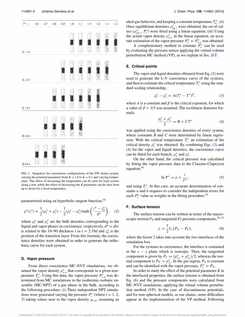
Some snapshots for equilibrated states are given inFigure 1, each line is related to a K value and the columns cor-respond to reduced temperatures. Density profiles were calcu-lated every MC cycle as a function of the long side of the box,z* = z/Lx.

To obtain vapor pressures we performed Monte Carlosimulations in the isothermic-isobaric ensemble (MC-NPT).A small cubic simulation box with N = 256 molecules wasused and the simulations were performed at very low values ofpressure (P* ∼ 10−2–10−3). Simulations required 1–5 × 106

cycles to equilibrate and 106 cycles to obtain averaged prop-erties. In Sec. II D, we detail the calculation of the vapor andcritical pressures from these NPT simulations.

A virtual volume perturbation was performed every NVTsimulation cycle to obtain the pressure tensor and surface ten-sion. To improve the statistical analysis, averages of pres-sure components were calculated after 64 × 106 configura-tions, divided in 8 independent simulations. As described ina previous work,47 a single volume perturbation parameter ξ

(=�V/V ) is enough for simulating discontinuous potentials;we selected ξ in such a way than around 30%–50% of ourvolume perturbation trials had a hard body overlap.

C. Density profiles

Profiles were obtained for monomers and moleculesas a function of the long side of the simulation box, and

Downloaded 17 Sep 2013 to 146.232.129.75. This article is copyrighted as indicated in the abstract. Reuse of AIP content is subject to the terms at: http://jcp.aip.org/about/rights_and_permissions

114901-3 Jiménez-Serratos et al. J. Chem. Phys. 139, 114901 (2013)

FIG. 1. Snapshots for coexistence configurations of the SW chains system,varying the potential parameter from K = 1.0 to K = 0.1 and varying temper-ature. The effect of increasing the temperature can be seen for each systemalong a row, while the effect of decreasing the K parameter can be seen fromup to down for a fixed temperature.

parametrized using an hyperbolic tangent function,48

ρ∗(z∗) = 1

2(ρ∗

l + ρ∗v ) − 1

2(ρ∗

l − ρ∗v ) tanh

(z∗ − z∗

0

d∗

), (2)

where ρ∗l and ρ∗

v are the bulk densities corresponding to theliquid and vapor phases in coexistence, respectively, d* = d/σis related to the 10–90 thickness t as t = 2.19d and z∗

0 is theposition of the transition layer. From this formula, the coexis-tence densities were obtained in order to generate the ortho-baric curve for each system.

D. Vapor pressure

From direct coexistence MC-NVT simulations, we ob-tained the vapor density ρ∗

v,a that corresponds to a given tem-perature T ∗

a . Using this data, the vapor pressure P ∗v,a was de-

termined from MC simulations in the isothermic-isobaric en-semble (MC-NPT) of a gas phase in the bulk, according tothe following procedure: (i) Three independent NPT simula-tions were generated varying the pressure P ∗

i (where i = 1, 2,3) taking values near to the vapor density ρv,a , assuming an

ideal gas behavior, and keeping a constant temperature T ∗a , (ii)

Once equilibrium densities ρ∗eq,i were obtained, the set of val-

ues (ρ∗eq,i , P

∗i ) were fitted using a linear equation; (iii) Using

the actual vapor density ρ∗v,a in the linear equation, an accu-

rate estimation of the vapor pressure P ∗v = P ∗

v,a was obtained.A complementary method to estimate P ∗

v can be usedby evaluating the pressure tensor applying the virtual-volumeperturbation MC method (VP), as we explain in Sec. II F.

E. Critical points

The vapor and liquid densities obtained from Eq. (2) wereused to generate the L-V coexistence curve of the systems,and then to estimate the critical temperature T ∗

c using the stan-dard scaling relationship,

ρ∗l − ρ∗

v = A(T ∗c − T ∗)β, (3)

where A is a constant and β is the critical exponent, for whicha value of β = 1/3 was assumed. The rectilinear diameter for-mula

ρ∗l + ρ∗

v

2= B + CT ∗ (4)

was applied using the coexistence densities of every system,where constants B and C were determined by linear regres-sion. With the critical temperature T ∗

c an estimation of thecritical density ρ∗

c was obtained. By combining Eqs. (3) and(4) for the vapor and liquid densities, the coexistence curvecan be fitted for each branch, ρ∗

v and ρ∗l .

On the other hand, the critical pressure was calculatedby fitting the vapor pressure data to the Clausius-Clapeyronequation,46

ln P ∗ = a + c

T ∗ , (5)

and using T ∗c . In this case, an accurate determination of con-

stants a and b requires to consider the independent errors foreach P ∗

v value as weights in the fitting procedure.49

F. Surface tension

The surface tension can be written in terms of the macro-scopic normal PN and tangential PT pressure components,50–52

γ = 1

2Lz[PN − PT ], (6)

where the factor 2 takes into account the two interfaces of thesimulation box.

For the systems in coexistence, the interface is containedin the x − y plane which is isotropic. Then, the tangentialcomponent is given by PT = (p∗

xx + p∗yy)/2, whereas the nor-

mal component is PN = p∗zz. In the gas region, PN is constant

and can be identified with the vapor pressure, P ∗v = PN .

In order to study the effect of the potential parameter K inthe interfacial properties, the surface tension is obtained fromEq. (6) and the pressure components were calculated fromMC-NVT simulations, applying the virtual volume perturba-tion method (VP). In the case of discontinuous potentials,and for non-spherical models, as our chains, some difficultiesappear in the implementation of the VP method. Following

Downloaded 17 Sep 2013 to 146.232.129.75. This article is copyrighted as indicated in the abstract. Reuse of AIP content is subject to the terms at: http://jcp.aip.org/about/rights_and_permissions

114901-4 Jiménez-Serratos et al. J. Chem. Phys. 139, 114901 (2013)

the method presented in our previous work,47 the pressure isgiven by

p = pideal + p(HB+SW )− + p

(HB)+ . (7)

The ideal contribution is pideal = NkBT/Vi , being Vi the un-perturbed volume of the NVT box. The second term corre-sponds to a compression contribution, denoted by the minussign,

p(HB+SW )− = lim

�Vi→j−→0

kBT

�Vi→j−ln

⟨exp

(−�U

(HB+SW )i→j−kBT

)⟩eq

.

(8)

The subscript j indicates a virtual state, obtained by perturb-ing the volume from Vi to Vj , so that �Vi→j− is the volumechange and �U

(HB+SW )i→j− is the energy difference between i

and j states. In this case, the label HB+SW emphasizes thatthe complete potential is taken into account. The third term inEq. (7) corresponds to an expansion contribution, denoted bya plus sign,

p(HB)+ = lim

�Vi→j+→0

kBT

�Vi→j+ln

⟨exp

(−�U

(HB)i→j+

kBT

)⟩eq

. (9)

Here, the notation is similar to the compression equation, butin this case only the HB interaction is taken into account.So, when a virtual volume expansion is performed, there arecontributions only from the few cases in which an HB over-lapping configuration is produced, as was shown by Brumbyet al. for non-spherical molecules.52

To evaluate the components of the pressure tensor, ananisotropic virtual change in volume is applied. If the compo-nent to calculate is pαα , for α = x, y, or z, then the simulationbox changes only its α size from Lα to Lα + �Lα . Finally, wedefine a volume perturbation parameter as ξ = �V/V , forthe anisotropic case it is given by ξ = �Lα/Lα .

III. RESULTS AND DISCUSSION

A. K �= 0 systems

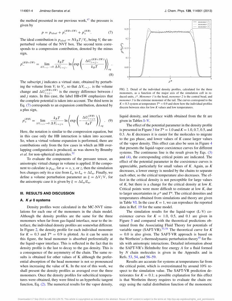
Density profiles were calculated in the MC-NVT simu-lations for each one of the monomers in the chain model.Although the density profiles are the same for the threemonomers when far from gas-liquid interface, near to the in-terface, the individual density profiles are somewhat different.In Figure 2, the density profile for each individual monomerfor K = 0.3 and T* = 0.9 is plotted. As it can be seen inthis figure, the head monomer is absorbed preferentially atthe liquid-vapor interface. This is reflected in the fact that itsdensity profile is the last to decay to the gas density. This isa consequence of the asymmetry of the chain. The same re-sults is obtained for other values of K although the prefer-ential absorption of the head monomer is not so pronouncedwhen increasing the value of K. In the rest of this work, weshall present the density profiles as averaged over the threemonomers. Once the density profiles for subcritical tempera-tures were obtained, they were fitted to an hyperbolic tangentfunction, Eq. (2). The numerical results for the vapor density,

2 4 6

z*0

0.05

0.1

0.15

0.2

0.25

ρ*(z

*)

monomer 1monomer 2monomer 3

FIG. 2. Detail of the individual density profiles, calculated for the threemonomers, as a function of the major axis of the simulation cell in re-duced units, z*. Monomer 1 is the head, monomer 2 is the central bead, andmonomer 3 is the extreme monomer of the tail. The curves correspond to theK = 0.3 system at temperature T* = 0.9 and show how the individual profilesdiscern between sites for low K values and low temperatures.

liquid density, and interface width obtained from the fit aregiven in Tables I–V.

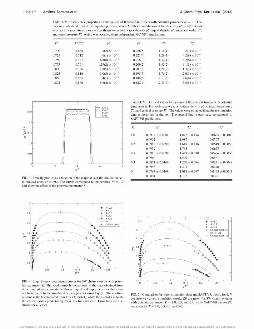
The effect of the potential parameter in the density profileis presented in Figure 3 for T* = 1.0 and K = 1.0, 0.7, 0.5, and0.3. As K decreases it is easier for the molecules to migrateto the gas phase, and lower values of K cause larger valuesof the vapor density. This effect can also be seen in Figure 4that presents the liquid-vapor coexistence curves for differentsystems. The continuous line is the result given by Eqs. (3)and (4), the corresponding critical points are indicated. Theeffect of the potential parameter in the coexistence curves isappreciable, particularly for small values of K. Again, as Kdecreases, a lower energy is needed by the chains to separateeach other, so the critical temperature also decreases. The ef-fect in the critical density is not perceptible for large valuesof K, but there is a change for the critical density at low K.Critical points were more difficult to estimate at low K, dueto larger uncertainties in ρ* and T*. The critical densities andtemperatures obtained from simulations and theory are givenin Table VI. In the case K = 1, we can reproduce the reporteddata in Ref. 19 for the same model.

The simulation results for the liquid-vapor (L-V) co-existence curves for K = 1.0, 0.5, and 0.1 are given inFigure 5 and compared with the theoretical predictions ob-tained from the Associating Fluid Theory for potentials ofvariable range (SAFT-VR).53, 54 The theoretical curve for K= 0.0 is also given. The SAFT-VR approach is based onthe Wertheim’;s thermodynamic perturbation theory55 for flu-ids with anisotropic interactions. Detailed information aboutthe SAFT-VR’s Helmholtz free energy A for a fluid formedby N chain molecules is given in the Appendix and inRefs. 53, 54, and 56–59.

Results are accurate for systems at temperatures far fromthe critical point, which is overestimated by around 10% re-spect to the simulation value. The SAFT-VR prediction de-teriorates for K = 0.1; a possible explanation for this effectis that Wertheim theory requires to evaluate the chain en-ergy using the radial distribution function of the monomeric

Downloaded 17 Sep 2013 to 146.232.129.75. This article is copyrighted as indicated in the abstract. Reuse of AIP content is subject to the terms at: http://jcp.aip.org/about/rights_and_permissions

114901-5 Jiménez-Serratos et al. J. Chem. Phys. 139, 114901 (2013)

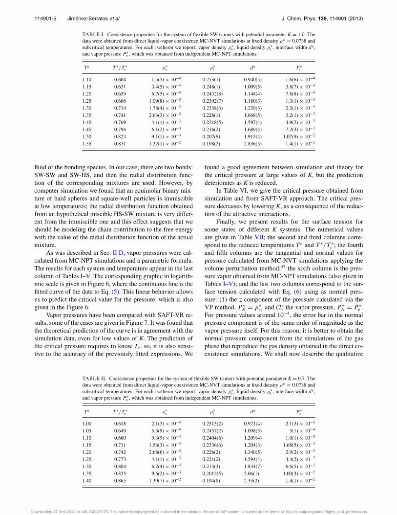
TABLE I. Coexistence properties for the system of flexible SW trimers with potential parameter K = 1.0. Thedata were obtained from direct liquid-vapor coexistence MC-NVT simulations at fixed density ρ* = 0.0738 andsubcritical temperatures. For each isotherm we report: vapor density ρ∗

v , liquid density ρ∗l , interface width d*,

and vapor pressure P ∗v , which was obtained from independent MC-NPT simulations.

T* T ∗/T ∗c ρ∗

v ρ∗l d* P ∗

v

1.10 0.604 1.5(5) × 10−4 0.253(1) 0.940(5) 1.6(6) × 10−4

1.15 0.631 3.4(5) × 10−4 0.248(1) 1.009(5) 3.8(7) × 10−4

1.20 0.659 6.7(5) × 10−4 0.2432(8) 1.148(4) 7.8(8) × 10−4

1.25 0.686 1.09(8) × 10−3 0.2392(7) 1.180(3) 1.3(1) × 10−3

1.30 0.714 1.78(4) × 10−3 0.2338(3) 1.229(3) 2.2(1) × 10−3

1.35 0.741 2.63(3) × 10−3 0.228(1) 1.668(5) 3.2(1) × 10−3

1.40 0.769 4.1(1) × 10−3 0.2218(5) 1.597(4) 4.9(2) × 10−3

1.45 0.796 6.1(2) × 10−3 0.216(2) 1.689(4) 7.2(3) × 10−3

1.50 0.823 9.1(1) × 10−3 0.207(9) 1.915(4) 1.07(9) × 10−2

1.55 0.851 1.22(1) × 10−2 0.198(2) 2.836(5) 1.4(1) × 10−2

fluid of the bonding species. In our case, there are two bonds:SW-SW and SW-HS, and then the radial distribution func-tion of the corresponding mixtures are used. However, bycomputer simulation we found that an equimolar binary mix-ture of hard spheres and square-well particles is immiscibleat low temperatures; the radial distribution function obtainedfrom an hypothetical miscible HS-SW mixture is very differ-ent from the immiscible one and this effect suggests that weshould be modeling the chain contribution to the free energywith the value of the radial distribution function of the actualmixture.

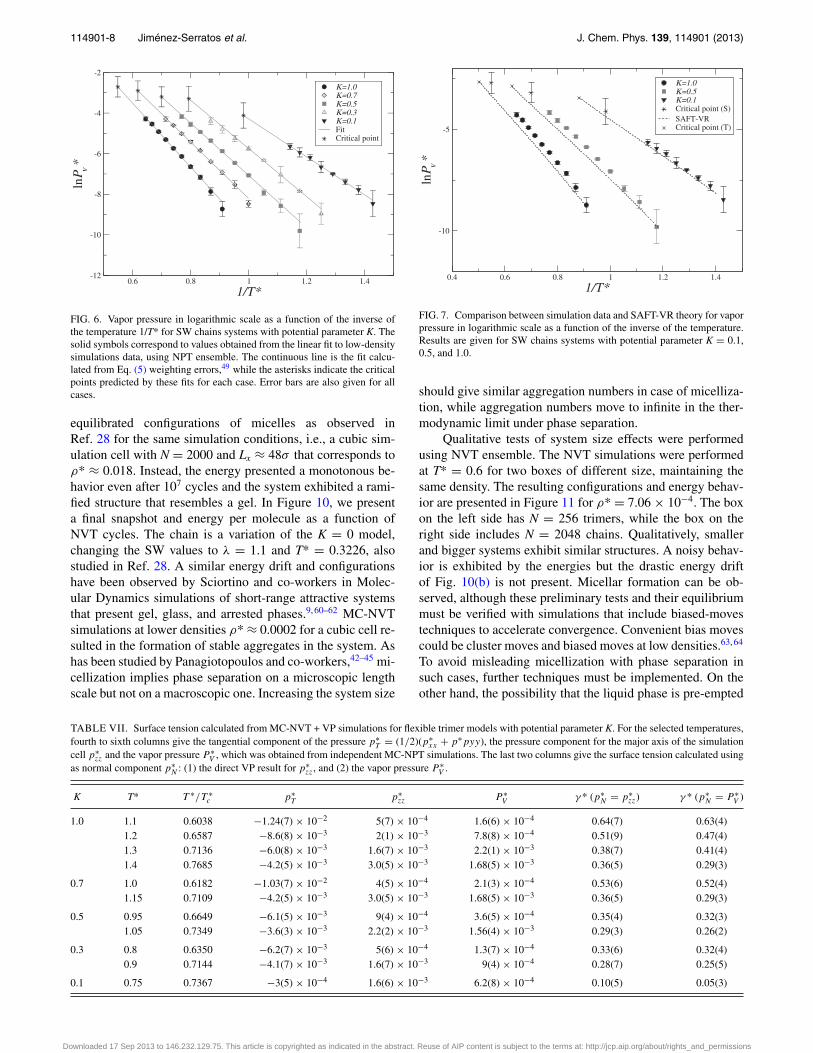
As was described in Sec. II D, vapor pressures were cal-culated from MC-NPT simulations and a parametric formula.The results for each system and temperature appear in the lastcolumn of Tables I–V. The corresponding graphic in logarith-mic scale is given in Figure 6, where the continuous line is thefitted curve of the data to Eq. (5). This linear behavior allowsus to predict the critical value for the pressure, which is alsogiven in the Figure 6.

Vapor pressures have been compared with SAFT-VR re-sults, some of the cases are given in Figure 7. It was found thatthe theoretical prediction of the curve is in agreement with thesimulation data, even for low values of K. The prediction ofthe critical pressure requires to know Tc, so, it is also sensi-tive to the accuracy of the previously fitted expressions. We

found a good agreement between simulation and theory forthe critical pressure at large values of K, but the predictiondeteriorates as K is reduced.

In Table VI, we give the critical pressure obtained fromsimulation and from SAFT-VR approach. The critical pres-sure decreases by lowering K, as a consequence of the reduc-tion of the attractive interactions.

Finally, we present results for the surface tension forsome states of different K systems. The numerical valuesare given in Table VII; the second and third columns corre-spond to the reduced temperatures T* and T ∗/T ∗

c ; the fourthand fifth columns are the tangential and normal values forpressure calculated from MC-NVT simulations applying thevolume perturbation method;47 the sixth column is the pres-sure vapor obtained from MC-NPT simulations (also given inTables I–V); and the last two columns correspond to the sur-face tension calculated with Eq. (6) using as normal pres-sure: (1) the z-component of the pressure calculated via theVP method, P ∗

N = p∗zz and (2) the vapor pressure, P ∗

N = P ∗v .

For pressure values around 10−4, the error bar in the normalpressure component is of the same order of magnitude as thevapor pressure itself. For this reason, it is better to obtain thenormal pressure component from the simulations of the gasphase that reproduce the gas density obtained in the direct co-existence simulations. We shall now describe the qualitative

TABLE II. Coexistence properties for the system of flexible SW trimers with potential parameter K = 0.7. Thedata were obtained from direct liquid-vapor coexistence MC-NVT simulations at fixed density ρ* = 0.0738 andsubcritical temperatures. For each isotherm we report: vapor density ρ∗

v , liquid density ρ∗l , interface width d*,

and vapor pressure P ∗v , which was obtained from independent MC-NPT simulations.

T* T ∗/T ∗c ρ∗

v ρ∗l d* P ∗

v

1.00 0.618 2.1(3) × 10−4 0.2515(2) 0.971(4) 2.1(3) × 10−4

1.05 0.649 5.3(9) × 10−4 0.2457(2) 1.098(3) 5(1) × 10−4

1.10 0.680 9.3(9) × 10−4 0.2404(6) 1.209(4) 1.0(1) × 10−3

1.15 0.711 1.56(3) × 10−3 0.2336(6) 1.204(3) 1.68(5) × 10−3

1.20 0.742 2.68(6) × 10−3 0.226(2) 1.340(5) 2.9(2) × 10−3

1.25 0.773 4.1(1) × 10−3 0.221(2) 1.594(4) 4.4(2) × 10−3

1.30 0.804 6.2(4) × 10−3 0.213(3) 1.834(7) 6.6(5) × 10−3

1.35 0.835 9.6(2) × 10−3 0.2012(5) 2.06(1) 1.00(3) × 10−2

1.40 0.865 1.39(7) × 10−2 0.194(8) 2.33(2) 1.4(1) × 10−2

Downloaded 17 Sep 2013 to 146.232.129.75. This article is copyrighted as indicated in the abstract. Reuse of AIP content is subject to the terms at: http://jcp.aip.org/about/rights_and_permissions

114901-6 Jiménez-Serratos et al. J. Chem. Phys. 139, 114901 (2013)

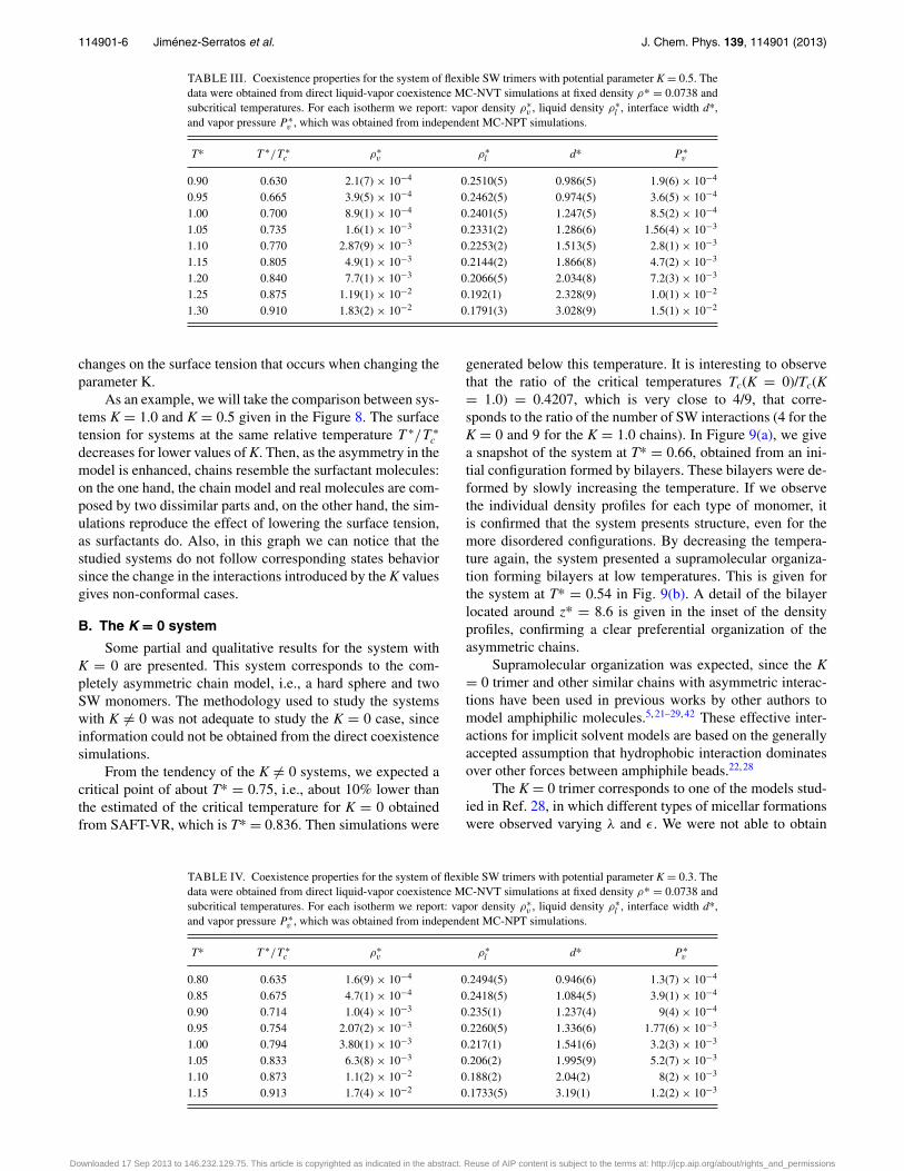
TABLE III. Coexistence properties for the system of flexible SW trimers with potential parameter K = 0.5. Thedata were obtained from direct liquid-vapor coexistence MC-NVT simulations at fixed density ρ* = 0.0738 andsubcritical temperatures. For each isotherm we report: vapor density ρ∗

v , liquid density ρ∗l , interface width d*,

and vapor pressure P ∗v , which was obtained from independent MC-NPT simulations.

T* T ∗/T ∗c ρ∗

v ρ∗l d* P ∗

v

0.90 0.630 2.1(7) × 10−4 0.2510(5) 0.986(5) 1.9(6) × 10−4

0.95 0.665 3.9(5) × 10−4 0.2462(5) 0.974(5) 3.6(5) × 10−4

1.00 0.700 8.9(1) × 10−4 0.2401(5) 1.247(5) 8.5(2) × 10−4

1.05 0.735 1.6(1) × 10−3 0.2331(2) 1.286(6) 1.56(4) × 10−3

1.10 0.770 2.87(9) × 10−3 0.2253(2) 1.513(5) 2.8(1) × 10−3

1.15 0.805 4.9(1) × 10−3 0.2144(2) 1.866(8) 4.7(2) × 10−3

1.20 0.840 7.7(1) × 10−3 0.2066(5) 2.034(8) 7.2(3) × 10−3

1.25 0.875 1.19(1) × 10−2 0.192(1) 2.328(9) 1.0(1) × 10−2

1.30 0.910 1.83(2) × 10−2 0.1791(3) 3.028(9) 1.5(1) × 10−2

changes on the surface tension that occurs when changing theparameter K.

As an example, we will take the comparison between sys-tems K = 1.0 and K = 0.5 given in the Figure 8. The surfacetension for systems at the same relative temperature T ∗/T ∗

c

decreases for lower values of K. Then, as the asymmetry in themodel is enhanced, chains resemble the surfactant molecules:on the one hand, the chain model and real molecules are com-posed by two dissimilar parts and, on the other hand, the sim-ulations reproduce the effect of lowering the surface tension,as surfactants do. Also, in this graph we can notice that thestudied systems do not follow corresponding states behaviorsince the change in the interactions introduced by the K valuesgives non-conformal cases.

B. The K = 0 system

Some partial and qualitative results for the system withK = 0 are presented. This system corresponds to the com-pletely asymmetric chain model, i.e., a hard sphere and twoSW monomers. The methodology used to study the systemswith K �= 0 was not adequate to study the K = 0 case, sinceinformation could not be obtained from the direct coexistencesimulations.

From the tendency of the K �= 0 systems, we expected acritical point of about T* = 0.75, i.e., about 10% lower thanthe estimated of the critical temperature for K = 0 obtainedfrom SAFT-VR, which is T* = 0.836. Then simulations were

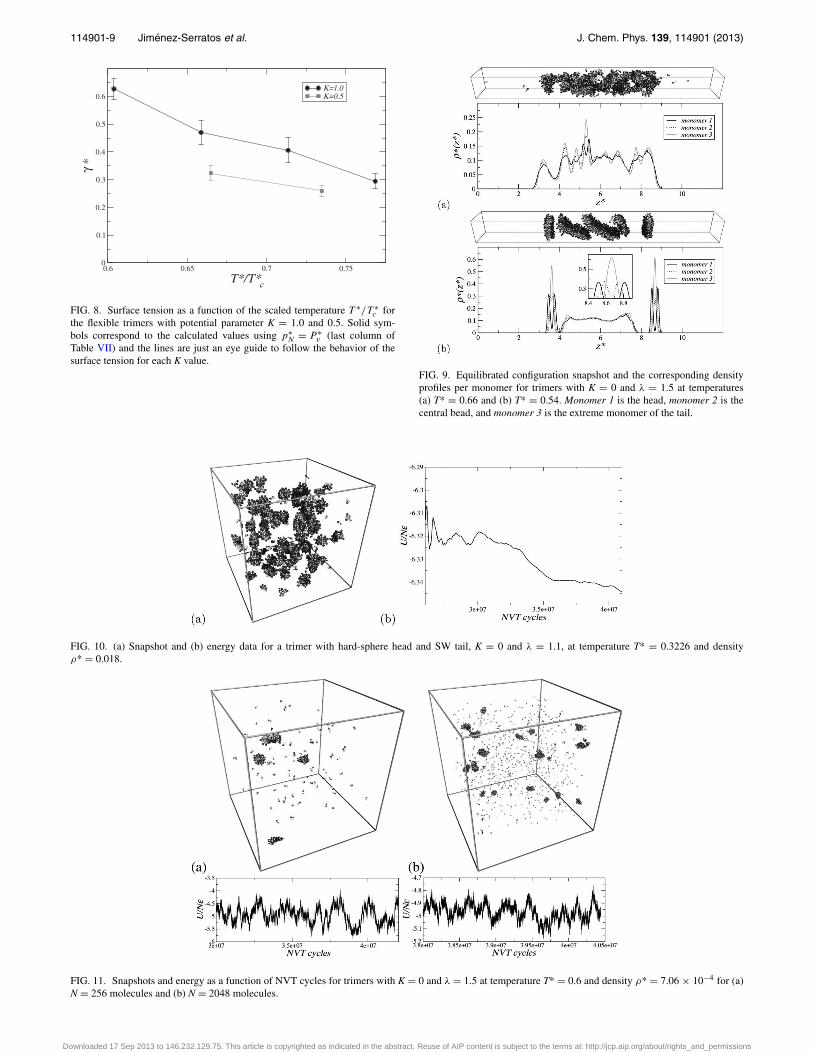
generated below this temperature. It is interesting to observethat the ratio of the critical temperatures Tc(K = 0)/Tc(K= 1.0) = 0.4207, which is very close to 4/9, that corre-sponds to the ratio of the number of SW interactions (4 for theK = 0 and 9 for the K = 1.0 chains). In Figure 9(a), we givea snapshot of the system at T* = 0.66, obtained from an ini-tial configuration formed by bilayers. These bilayers were de-formed by slowly increasing the temperature. If we observethe individual density profiles for each type of monomer, itis confirmed that the system presents structure, even for themore disordered configurations. By decreasing the tempera-ture again, the system presented a supramolecular organiza-tion forming bilayers at low temperatures. This is given forthe system at T* = 0.54 in Fig. 9(b). A detail of the bilayerlocated around z* = 8.6 is given in the inset of the densityprofiles, confirming a clear preferential organization of theasymmetric chains.

Supramolecular organization was expected, since the K= 0 trimer and other similar chains with asymmetric interac-tions have been used in previous works by other authors tomodel amphiphilic molecules.5, 21–29, 42 These effective inter-actions for implicit solvent models are based on the generallyaccepted assumption that hydrophobic interaction dominatesover other forces between amphiphile beads.22, 28

The K = 0 trimer corresponds to one of the models stud-ied in Ref. 28, in which different types of micellar formationswere observed varying λ and ε. We were not able to obtain

TABLE IV. Coexistence properties for the system of flexible SW trimers with potential parameter K = 0.3. Thedata were obtained from direct liquid-vapor coexistence MC-NVT simulations at fixed density ρ* = 0.0738 andsubcritical temperatures. For each isotherm we report: vapor density ρ∗

v , liquid density ρ∗l , interface width d*,

and vapor pressure P ∗v , which was obtained from independent MC-NPT simulations.

T* T ∗/T ∗c ρ∗

v ρ∗l d* P ∗

v

0.80 0.635 1.6(9) × 10−4 0.2494(5) 0.946(6) 1.3(7) × 10−4

0.85 0.675 4.7(1) × 10−4 0.2418(5) 1.084(5) 3.9(1) × 10−4

0.90 0.714 1.0(4) × 10−3 0.235(1) 1.237(4) 9(4) × 10−4

0.95 0.754 2.07(2) × 10−3 0.2260(5) 1.336(6) 1.77(6) × 10−3

1.00 0.794 3.80(1) × 10−3 0.217(1) 1.541(6) 3.2(3) × 10−3

1.05 0.833 6.3(8) × 10−3 0.206(2) 1.995(9) 5.2(7) × 10−3

1.10 0.873 1.1(2) × 10−2 0.188(2) 2.04(2) 8(2) × 10−3

1.15 0.913 1.7(4) × 10−2 0.1733(5) 3.19(1) 1.2(2) × 10−3

Downloaded 17 Sep 2013 to 146.232.129.75. This article is copyrighted as indicated in the abstract. Reuse of AIP content is subject to the terms at: http://jcp.aip.org/about/rights_and_permissions

114901-7 Jiménez-Serratos et al. J. Chem. Phys. 139, 114901 (2013)

TABLE V. Coexistence properties for the system of flexible SW trimers with potential parameter K = 0.1. Thedata were obtained from direct liquid-vapor coexistence MC-NVT simulations at fixed density ρ* = 0.0738 andsubcritical temperatures. For each isotherm we report: vapor density ρ∗

v , liquid density ρ∗l , interface width d*,

and vapor pressure P ∗v , which was obtained from independent MC-NPT simulations.

T* T ∗/T ∗c ρ∗

v ρ∗l d* P ∗

v

0.700 0.688 3(2) × 10−4 0.226(5) 1.16(1) 2(1) × 10−4

0.725 0.712 6(1) × 10−4 0.221(4) 1.29(1) 4.2(9) × 10−4

0.750 0.737 8.8(8) × 10−4 0.218(3) 1.32(1) 6.2(8) × 10−4

0.775 0.761 1.29(2) × 10−3 0.209(2) 1.42(2) 9.1(3) × 10−4

0.800 0.786 1.8(5) × 10−3 0.201(6) 1.28(2) 1.3(3) × 10−3

0.825 0.810 3.0(3) × 10−3 0.195(5) 1.76(2) 2.0(3) × 10−3

0.850 0.835 4(1) × 10−3 0.188(6) 2.13(2) 2.6(6) × 10−3

0.875 0.860 5.6(4) × 10−3 0.182(9) 2.47(4) 3.5(5) × 10−3

0 2 4 6 8

z*0

0.05

0.1

0.15

0.2

0.25

ρ*(z

*)

K=1.0K=0.7K=0.5K=0.3

FIG. 3. Density profiles as a function of the major axis of the simulation cellin reduced units, z* = z/Lx. The curves correspond to temperature T* = 1.0and show the effect of the potential parameter K.

0 0.05 0.1 0.15 0.2 0.25ρ∗

0.8

1

1.2

1.4

1.6

1.8

2

T*

K=1.0K=0.7K=0.5K=0.3K=0.1FitCritical point

FIG. 4. Liquid-vapor coexistence curves for SW chains systems with poten-tial parameter K. The solid symbols correspond to the data obtained fromdirect coexistence simulations, this is, liquid and vapor densities that cameout from the fit to the simulated density profiles using Eq. (2). The continu-ous line is the fit calculated from Eqs. (3) and (4), while the asterisks indicatethe critical points predicted by these fits for each case. Error bars are alsoshown for all cases.

TABLE VI. Critical values for systems of flexible SW trimers with potentialparameter K. For each case we give: critical density ρ∗

c , critical temperatureT ∗

c , and critical pressure P ∗c . The values were obtained from fits to simulation

data as described in the text. The second line in each case corresponds toSAFT-VR predictions.

K ρ∗c T ∗

c P ∗c

1.0 0.0932 ± 0.0081 1.822 ± 0.114 0.0665 ± 0.00800.0952 1.987 0.0707

0.7 0.0912 ± 0.0099 1.618 ± 0.116 0.0549 ± 0.00500.0959 1.765 0.0627

0.5 0.0910 ± 0.0098 1.429 ± 0.070 0.0406 ± 0.00300.0960 1.599 0.0561

0.3 0.0871 ± 0.0166 1.260 ± 0.094 0.0371 ± 0.00480.0953 1.401 0.0470

0.1 0.0767 ± 0.0198 1.018 ± 0.097 0.0163 ± 0.00110.0894 1.132 0.0321

0 0.05 0.1 0.15 0.2 0.25ρ∗

0.6

0.8

1

1.2

1.4

1.6

1.8

2

T*

K=1.0K=0.5K=0.1Critical point (S)SAFT-VRCritical point (T)

FIG. 5. Comparison between simulation data and SAFT-VR theory for L-Vcoexistence curves. Simulation results (S) are given for SW chains systemswith potential parameter K = 1.0, 0.5, and 0.1, while SAFT-VR curves (T)are given for K = 1.0, 0.5, 0.1, and 0.0.

Downloaded 17 Sep 2013 to 146.232.129.75. This article is copyrighted as indicated in the abstract. Reuse of AIP content is subject to the terms at: http://jcp.aip.org/about/rights_and_permissions

114901-8 Jiménez-Serratos et al. J. Chem. Phys. 139, 114901 (2013)

0.6 0.8 1 1.2 1.4

1/T*-12

-10

-8

-6

-4

-2ln

P v*

K=1.0K=0.7K=0.5K=0.3K=0.1FitCritical point

FIG. 6. Vapor pressure in logarithmic scale as a function of the inverse ofthe temperature 1/T* for SW chains systems with potential parameter K. Thesolid symbols correspond to values obtained from the linear fit to low-densitysimulations data, using NPT ensemble. The continuous line is the fit calcu-lated from Eq. (5) weighting errors,49 while the asterisks indicate the criticalpoints predicted by these fits for each case. Error bars are also given for allcases.

equilibrated configurations of micelles as observed inRef. 28 for the same simulation conditions, i.e., a cubic sim-ulation cell with N = 2000 and Lx ≈ 48σ that corresponds toρ* ≈ 0.018. Instead, the energy presented a monotonous be-havior even after 107 cycles and the system exhibited a rami-fied structure that resembles a gel. In Figure 10, we presenta final snapshot and energy per molecule as a function ofNVT cycles. The chain is a variation of the K = 0 model,changing the SW values to λ = 1.1 and T* = 0.3226, alsostudied in Ref. 28. A similar energy drift and configurationshave been observed by Sciortino and co-workers in Molec-ular Dynamics simulations of short-range attractive systemsthat present gel, glass, and arrested phases.9, 60–62 MC-NVTsimulations at lower densities ρ* ≈ 0.0002 for a cubic cell re-sulted in the formation of stable aggregates in the system. Ashas been studied by Panagiotopoulos and co-workers,42–45 mi-cellization implies phase separation on a microscopic lengthscale but not on a macroscopic one. Increasing the system size

0.4 0.6 0.8 1 1.2 1.4

1/T*

-10

-5

lnP v

*

K=1.0K=0.5K=0.1Critical point (S)SAFT-VRCritical point (T)

FIG. 7. Comparison between simulation data and SAFT-VR theory for vaporpressure in logarithmic scale as a function of the inverse of the temperature.Results are given for SW chains systems with potential parameter K = 0.1,0.5, and 1.0.

should give similar aggregation numbers in case of micelliza-tion, while aggregation numbers move to infinite in the ther-modynamic limit under phase separation.

Qualitative tests of system size effects were performedusing NVT ensemble. The NVT simulations were performedat T* = 0.6 for two boxes of different size, maintaining thesame density. The resulting configurations and energy behav-ior are presented in Figure 11 for ρ* = 7.06 × 10−4. The boxon the left side has N = 256 trimers, while the box on theright side includes N = 2048 chains. Qualitatively, smallerand bigger systems exhibit similar structures. A noisy behav-ior is exhibited by the energies but the drastic energy driftof Fig. 10(b) is not present. Micellar formation can be ob-served, although these preliminary tests and their equilibriummust be verified with simulations that include biased-movestechniques to accelerate convergence. Convenient bias movescould be cluster moves and biased moves at low densities.63, 64

To avoid misleading micellization with phase separation insuch cases, further techniques must be implemented. On theother hand, the possibility that the liquid phase is pre-empted

TABLE VII. Surface tension calculated from MC-NVT + VP simulations for flexible trimer models with potential parameter K. For the selected temperatures,fourth to sixth columns give the tangential component of the pressure p∗

T = (1/2)(p∗xx + p∗pyy), the pressure component for the major axis of the simulation

cell p∗zz and the vapor pressure P ∗

V , which was obtained from independent MC-NPT simulations. The last two columns give the surface tension calculated usingas normal component p∗

N : (1) the direct VP result for p∗zz, and (2) the vapor pressure P ∗

V .

K T* T ∗/T ∗c p∗

T p∗zz P ∗

V γ * (p∗N = p∗

zz) γ * (p∗N = P ∗

V )

1.0 1.1 0.6038 −1.24(7) × 10−2 5(7) × 10−4 1.6(6) × 10−4 0.64(7) 0.63(4)1.2 0.6587 −8.6(8) × 10−3 2(1) × 10−3 7.8(8) × 10−4 0.51(9) 0.47(4)1.3 0.7136 −6.0(8) × 10−3 1.6(7) × 10−3 2.2(1) × 10−3 0.38(7) 0.41(4)1.4 0.7685 −4.2(5) × 10−3 3.0(5) × 10−3 1.68(5) × 10−3 0.36(5) 0.29(3)

0.7 1.0 0.6182 −1.03(7) × 10−2 4(5) × 10−4 2.1(3) × 10−4 0.53(6) 0.52(4)1.15 0.7109 −4.2(5) × 10−3 3.0(5) × 10−3 1.68(5) × 10−3 0.36(5) 0.29(3)

0.5 0.95 0.6649 −6.1(5) × 10−3 9(4) × 10−4 3.6(5) × 10−4 0.35(4) 0.32(3)1.05 0.7349 −3.6(3) × 10−3 2.2(2) × 10−3 1.56(4) × 10−3 0.29(3) 0.26(2)

0.3 0.8 0.6350 −6.2(7) × 10−3 5(6) × 10−4 1.3(7) × 10−4 0.33(6) 0.32(4)0.9 0.7144 −4.1(7) × 10−3 1.6(7) × 10−3 9(4) × 10−4 0.28(7) 0.25(5)

0.1 0.75 0.7367 −3(5) × 10−4 1.6(6) × 10−3 6.2(8) × 10−4 0.10(5) 0.05(3)

Downloaded 17 Sep 2013 to 146.232.129.75. This article is copyrighted as indicated in the abstract. Reuse of AIP content is subject to the terms at: http://jcp.aip.org/about/rights_and_permissions

114901-9 Jiménez-Serratos et al. J. Chem. Phys. 139, 114901 (2013)

0.6 0.65 0.7 0.75

T*/T*c

0

0.1

0.2

0.3

0.4

0.5

0.6γ

∗K=1.0K=0.5

FIG. 8. Surface tension as a function of the scaled temperature T ∗/T ∗c for

the flexible trimers with potential parameter K = 1.0 and 0.5. Solid sym-bols correspond to the calculated values using p∗

N = P ∗v (last column of

Table VII) and the lines are just an eye guide to follow the behavior of thesurface tension for each K value.

FIG. 9. Equilibrated configuration snapshot and the corresponding densityprofiles per monomer for trimers with K = 0 and λ = 1.5 at temperatures(a) T* = 0.66 and (b) T* = 0.54. Monomer 1 is the head, monomer 2 is thecentral bead, and monomer 3 is the extreme monomer of the tail.

FIG. 10. (a) Snapshot and (b) energy data for a trimer with hard-sphere head and SW tail, K = 0 and λ = 1.1, at temperature T* = 0.3226 and densityρ* = 0.018.

FIG. 11. Snapshots and energy as a function of NVT cycles for trimers with K = 0 and λ = 1.5 at temperature T* = 0.6 and density ρ* = 7.06 × 10−4 for (a)N = 256 molecules and (b) N = 2048 molecules.

Downloaded 17 Sep 2013 to 146.232.129.75. This article is copyrighted as indicated in the abstract. Reuse of AIP content is subject to the terms at: http://jcp.aip.org/about/rights_and_permissions

114901-10 Jiménez-Serratos et al. J. Chem. Phys. 139, 114901 (2013)

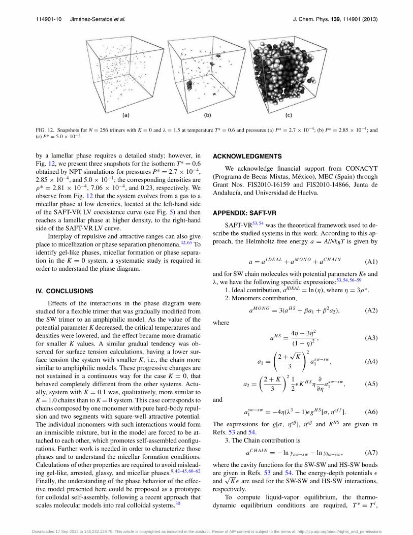
FIG. 12. Snapshots for N = 256 trimers with K = 0 and λ = 1.5 at temperature T* = 0.6 and pressures (a) P* = 2.7 × 10−4; (b) P* = 2.85 × 10−4; and(c) P* = 5.0 × 10−1.

by a lamellar phase requires a detailed study; however, inFig. 12, we present three snapshots for the isotherm T* = 0.6obtained by NPT simulations for pressures P* = 2.7 × 10−4,2.85 × 10−4, and 5.0 × 10−1; the corresponding densities areρ* = 2.81 × 10−4, 7.06 × 10−4, and 0.23, respectively. Weobserve from Fig. 12 that the system evolves from a gas to amicellar phase at low densities, located at the left-hand sideof the SAFT-VR LV coexistence curve (see Fig. 5) and thenreaches a lamellar phase at higher density, to the right-handside of the SAFT-VR LV curve.

Interplay of repulsive and attractive ranges can also giveplace to micellization or phase separation phenomena.42, 65 Toidentify gel-like phases, micellar formation or phase separa-tion in the K = 0 system, a systematic study is required inorder to understand the phase diagram.

IV. CONCLUSIONS

Effects of the interactions in the phase diagram werestudied for a flexible trimer that was gradually modified fromthe SW trimer to an amphiphilic model. As the value of thepotential parameter K decreased, the critical temperatures anddensities were lowered, and the effect became more dramaticfor smaller K values. A similar gradual tendency was ob-served for surface tension calculations, having a lower sur-face tension the system with smaller K, i.e., the chain moresimilar to amphiphilic models. These progressive changes arenot sustained in a continuous way for the case K = 0, thatbehaved completely different from the other systems. Actu-ally, system with K = 0.1 was, qualitatively, more similar toK = 1.0 chains than to K = 0 system. This case corresponds tochains composed by one monomer with pure hard-body repul-sion and two segments with square-well attractive potential.The individual monomers with such interactions would forman immiscible mixture, but in the model are forced to be at-tached to each other, which promotes self-assembled configu-rations. Further work is needed in order to characterize thosephases and to understand the micellar formation conditions.Calculations of other properties are required to avoid mislead-ing gel-like, arrested, glassy, and micellar phases.9, 42–45, 60–62

Finally, the understanding of the phase behavior of the effec-tive model presented here could be proposed as a prototypefor colloidal self-assembly, following a recent approach thatscales molecular models into real colloidal systems.30

ACKNOWLEDGMENTS

We acknowledge financial support from CONACYT(Programa de Becas Mixtas, México), MEC (Spain) throughGrant Nos. FIS2010-16159 and FIS2010-14866, Junta deAndalucía, and Universidad de Huelva.

APPENDIX: SAFT-VR

SAFT-VR53, 54 was the theoretical framework used to de-scribe the studied systems in this work. According to this ap-proach, the Helmholtz free energy a = A/NkBT is given by

a = aIDEAL + aMONO + aCHAIN (A1)

and for SW chain molecules with potential parameters Kε andλ, we have the following specific expressions:53, 54, 56–59

1. Ideal contribution, aIDEAL = ln (η), where η = 3ρ*.2. Monomers contribution,

aMONO = 3(aHS + βa1 + β2a2), (A2)

where

aHS = 4η − 3η2

(1 − η)2 , (A3)

a1 =(

2 + √K

3

)2

asw−sw1 , (A4)

a2 =(

2 + K

3

)2 1

2εKHSη

∂

∂ηasw−sw

1 , (A5)

and

asw−sw1 = −4η(λ3 − 1)εgHS[σ, ηeff ]. (A6)

The expressions for g[σ , ηeff], ηeff and KHS are given inRefs. 53 and 54.

3. The Chain contribution is

aCHAIN = − ln ysw−sw − ln yhs−sw, (A7)

where the cavity functions for the SW-SW and HS-SW bondsare given in Refs. 53 and 54. The energy-depth potentials ε

and√

Kε are used for the SW-SW and HS-SW interactions,respectively.

To compute liquid-vapor equilibrium, the thermo-dynamic equilibrium conditions are required, T v = T l ,

Downloaded 17 Sep 2013 to 146.232.129.75. This article is copyrighted as indicated in the abstract. Reuse of AIP content is subject to the terms at: http://jcp.aip.org/about/rights_and_permissions

114901-11 Jiménez-Serratos et al. J. Chem. Phys. 139, 114901 (2013)

P v = T l , and μv = μl , where v and l denote vapor and liq-uid phases. The chemical potential and pressure are obtainedusing Eq. (A1) and the thermodynamic relations

μ =(

∂A

∂N

)T ,V

= a + η

(∂a

∂η

)T ,V

, (A8)

and

Z = P

NkBT= η

(∂a

∂η

)T ,V

, (A9)

where Z is the compressibility factor.

1Y. S. Velichko, S. I. Stupp, and M. O. de la Cruz, J. Phys. Chem. B 112,2326 (2008).

2C. Avendaño, A. Gil-Villegas, and E. González-Tovar, Chem. Phys. Lett.470, 67 (2009).

3A. J. Crane, F. J. Martínez-Veracoechea, F. A. Escobedo, and E. A. Müller,Soft Matter 4, 1820 (2008).

4M. Sammalkorpi, S. Sanders, A. Z. Panagiotopoulos, M. Karttunen, and M.Haataja, J. Phys. Chem. B 115, 1403 (2011).

5S. V. Burov and A. K. Shchekin, J. Chem. Phys. 133, 244109 (2010).6C. McBride and C. Vega, J. Chem. Phys. 117, 10370 (2002).7C. McBride, C. Vega, and L. G. MacDowell, Phys. Rev. E 64, 011703(2001).

8S. Puvvada and D. Blankschtein, J. Chem. Phys. 92, 3710 (1990).9G. Foffi, C. De Michele, F. Sciortino, and P. Tartaglia, J. Chem. Phys. 122,224903 (2005).

10A. Jusufi, A.-P. Hynninen, and A. Z. Panagiotopoulos, J. Phys. Chem. B112, 13783 (2008).

11A. T. Bernardes, V. B. Henriques, and P. M. Bisch, J. Chem. Phys. 101, 645(1994).

12Z. Wang and R. G. Larson, J. Phys. Chem. B 113, 13697 (2009).13S. J. Marrink, D. P. Tieleman, and A. E. Mark, J. Phys. Chem. B 104, 12165

(2000).14J. L. Woodhead and C. K. Hall, Langmuir 26, 15135 (2010).15B. C. Stephenson, K. J. Beers, and D. Blankschtein, J. Phys. Chem. B 111,

1063 (2007).16R. Pool and P. G. Bolhuis, Phys. Chem. Chem. Phys. 8, 941 (2006).17L. Vega, E. de Miguel, L. F. Rull, G. Jackson, and I. A. McLure, J. Chem.

Phys. 96, 2296 (1992).18A. Giacometti, G. Pastore, and F. Lado, Mol. Phys. 107, 555 (2009).19S. V. Fridrikh and J. E. G. Lipson, J. Chem. Phys. 116, 8483 (2002).20A. P. Malanoski and P. A. Monson, J. Chem. Phys. 107, 6899 (1997).21R. G. Larson, J. Chem. Phys. 91, 2479 (1989).22J. Huang, Y. Wang, and C. Qian, J. Chem. Phys. 131, 234902 (2009).23S. Fujiwara, T. Itoh, M. Hashimoto, and R. Horiuchi, J. Chem. Phys. 130,

144901 (2009).24D. Bedrov, G. D. Smith, K. F. Freed, and J. Dudowicz, J. Chem. Phys. 116,

4765 (2002).25S. Tsonchev, G. C. Schatz, and M. A. Ratner, J. Phys. Chem. B 108, 8817

(2004).26G. K. Bourov and A. Bhattacharya, J. Chem. Phys. 122, 044702 (2005).27G. Brannigan, Phys. Rev. E 72, 011915 (2005).28T. Zehl, M. Wahab, H.-J. Mögel, and P. Schiller, Langmuir 22, 2523

(2006).29T. Zehl, M. Wahab, H.-J. Mögel, and P. Schiller, Langmuir 25, 7313 (2009).30F. Romano and F. Sciortino, Nature Mater. 10, 171 (2011).

31E. Zaccarelli, S. V. Buldyrev, E. La Nave, A. J. Moreno, Saika-Voivod, F.Sciortino, and P. Tartaglia, Phys. Rev. Lett. 94, 218301 (2005).

32E. Bianchi, J. largo, P. Tartaglia, E. Zaccarelli, and F. Sciortino, Phys. Rev.Lett. 97, 168301 (2006).

33F. Sciortino, Eur. Phys. J. B 64, 505 (2008).34R. P. Sear, S. Chung, G. Markovich, W. M. Gelbart, and J. R. Heath, Phys.

Rev. E 59, R6255 (1999).35S. Mejía-Rosales, A. Gil-Villegas, B. Ivlev, and J. Ruíz-García, J. Phys.:

Condens. Matter 14, 4795 (2002).36S. Mejía-Rosales, A. Gil-Villegas, B. Ivlev, and J. Ruíz-García, J. Phys.

Chem. B 110, 22230 (2006).37K.-H. Roh and D. C. Martin, J. Lahann, Nature Mater. 4, 759 (2005).38A. Walther and A. H. E. Müller, Soft Matter 4, 663 (2008).39B. J. Park, C.-H Choi, S.-M. Kang, K. E. Tettey, C.-S. Lee, and D. Lee,

Langmuir 29, 1841 (2013).40A. Walther and A. H. E. Müller, Chem. Rev. 113, 5194 (2013).41F. Sciortino, A. Giacometti, and G. Pastore, Phys. Rev. Lett. 103, 237801

(2009).42S. Salaniwal, S. K. Kumar, and A. Z. Panagiotopoulos, Langmuir 19, 5164

(2003).43A. D. Mackie, K. Onur, and A. Z. Panagiotopoulos, J. Chem. Phys. 104,

3718 (1996).44A. D. Mackie and A. Z. Panagiotopoulos, Langmuir 13, 5022 (1997).45M. A. Floriano, E. Caponetti, and A. Z. Panagiotopoulos, Langmuir 15,

3143 (1999).46J. S. Rowlinson and F. L. Swinton, Liquids and Liquid Mixtures, 3rd ed.

(Butterworth Scientific, London, UK, 1982).47G. Jiménez-Serratos, C. Vega, and A. Gil-Villegas, J. Chem. Phys. 137,

204104 (2012).48J. W. Cahn and J. E. Hilliard, J. Chem. Phys. 28, 258 (1958).49W. H. Press, S. A. Teukolsky, W. T. Vetterling, and B. P. Flannery,

Numerical Recipes in Fortran 90, 2nd ed. (Cambridge University Press,Cambridge, UK, 1996).

50E. de Miguel and G. Jackson, J. Chem. Phys. 125, 164109 (2006).51E. de Miguel, J. Phys. Chem. B 112, 4674 (2008).52P. E. Brumby, A. J. Haslam, E. de Miguel, and G. Jackson, Mol. Phys. 109,

169 (2011).53A. Gil-Villegas, A. Galindo, P. J. Whitehead, S. J. Mills, G. Jackson, and

A. N. Burgess, J. Chem. Phys. 106, 4168 (1997).54A. Galindo, L. A. Davies, A. Gil-Villegas, and G. Jackson, Mol. Phys. 93,

241 (1998).55M. S. Wertheim, J. Stat. Phys. 35, 19 (1984); 35, 35 (1984); 42, 459 (1986);

42, 477 (1986); J. Chem. Phys. 85, 2929 (1986); 87, 7323 (1987).56Y. Peng, H. Zhao, and C. McCabe, Mol. Phys. 104, 571 (2006).57M. C. dos Ramos and F. J. Blas, Mol. Phys. 105, 1319 (2007).58P. Morgado, H. Zhao, F. J. Blas, C. McCabe, L. P. N. Rebelo, and E. J. M.

Filipe, J. Phys. Chem. B 111, 2856 (2007).59P. Morgado, R. Tomás, H. Zhao, M. C. dos Ramos, F. J. Blas, C. McCabe,

and E. J. M. Filipe, J. Phys. Chem. C 111, 15962 (2007).60F. Sciortino, Nature Mater. 1, 145 (2002).61G. Foffi, E. Zaccarelli, S. Buldyrev, F. Sciortino, and P. Tartaglia, J. Chem.

Phys. 120, 8824 (2004).62J. C. F. Toledano, F. Sciortino, and E. Zaccarelli, Soft Matter 5, 2390

(2009).63D. Frenkel and B. Smit, Understanding Molecular Simulation (Academic

Press, London, 2002).64C. Valeriani, P. J. Camp, J. W. Zwaninkken, R. van Roij, and M. Dijkstra,

J. Phys.: Condens. Matter 22, 104112 (2010).65V. Kapila, J. M. Harris, P. A. Deymier, and S. Raghavan, Langmuir 18,

3728 (2002).

Downloaded 17 Sep 2013 to 146.232.129.75. This article is copyrighted as indicated in the abstract. Reuse of AIP content is subject to the terms at: http://jcp.aip.org/about/rights_and_permissions