FLUKA Beginner’s Course

Monte Carlo sampling

Overview: General concepts:

Phase space

The Boltzmann equation

Monte Carlo foundations

Simulation vs. integration

Sampling techniques

discrete

by inversion

by rejection

Results and Errors:

Statistical errors (single histories, batches)

Figure of merit

Phase space: Phase space: a concept of classical Statistical Mechanics

Each Phase Space dimension corresponds to a particle degree of

freedom

3 dimensions correspond to Position in (real) space: x, y, z

3 dimensions correspond to Momentum: px, py, pz

(or Energy and direction: E, , )

More dimensions may be envisaged, corresponding to other possible

degrees of freedom, such as quantum numbers: spin, etc.

Another degree of freedom is the particle type itself (electron,

proton...)

Each particle is represented by a point in phase space

Time can also be considered as a coordinate, or it can be

considered as an independent variable: the variation of the other

phase space coordinates as a function of time constitutes a

particle “history”

The angular flux Ψ

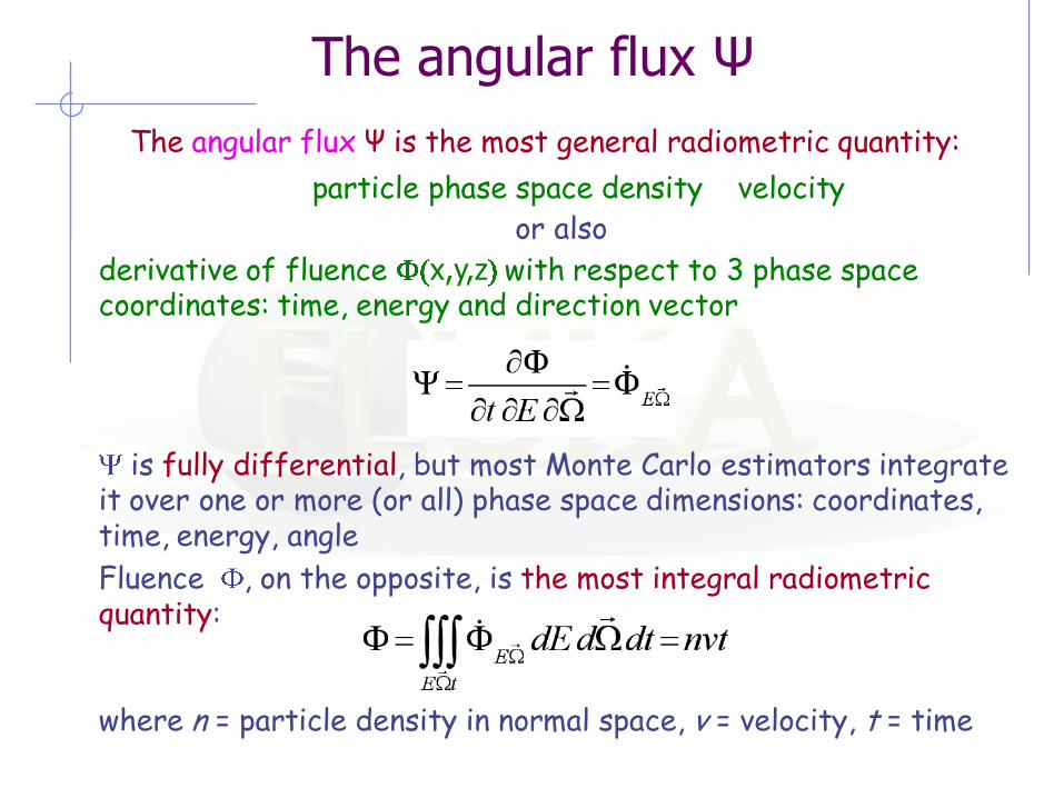
The angular flux Ψ is the most general radiometric quantity:

particle phase space density velocity or also

derivative of fluence x,y,z with respect to 3 phase space coordinates: time, energy and direction vector

is fully differential, but most Monte Carlo estimators integrate it over one or more (or all) phase space dimensions: coordinates, time, energy, angle

Fluence , on the opposite, is the most integral radiometric quantity:

where n = particle density in normal space, v = velocity, t = time

The Boltzmann Equation

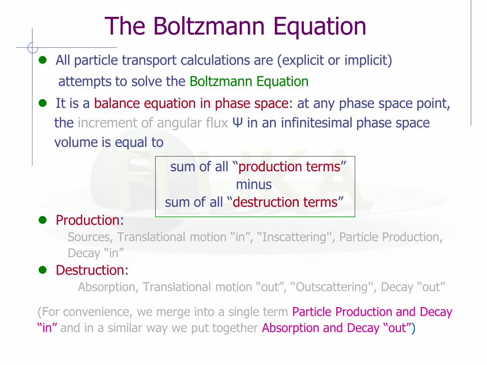
All particle transport calculations are (explicit or implicit)

attempts to solve the Boltzmann Equation

It is a balance equation in phase space: at any phase space point,

the increment of angular flux Ψ in an infinitesimal phase space

volume is equal to

sum of all “production terms”

minus

sum of all “destruction terms”

Production: Sources, Translational motion “in”, “Inscattering'', Particle Production,

Decay “in”

Destruction: Absorption, Translational motion “out”, “Outscattering'', Decay “out”

(For convenience, we merge into a single term Particle Production and Decay

“in” and in a similar way we put together Absorption and Decay “out”)

The Boltzmann Equation

''),',';(),,,(),,,(1

ddEEErtErStErtv

st

t = total macroscopic cross section = interaction probability per cm

= 1/ t = tNA /A

t = interaction mean free path t = interaction probability per atom/cm2

s = scattering macroscopic cross section = sNA /A

This equation is in integro-differential form. But in Monte Carlo it is more convenient to put it into integral form, carrying out the integration over all possible particle histories.

A theorem of statistical mechanics, the Ergodic Theorem, says that the average of a function along the trajectories is equal to the average over all phase space. The trajectories “fill” all the available phase space.

time dependent absorption source translation

scattering

Visualizing a 2-D phase space...

pE

,

r

Translational motion: change of position, no change of energy and direction

Scattering: no change of position, change of energy and direction

In Out

Inscattering Outscattering

dE/dx: change of position and energy (translation plus many small scatterings

No arrows upwards! (except for thermal neutrons)

The sources and the detectors

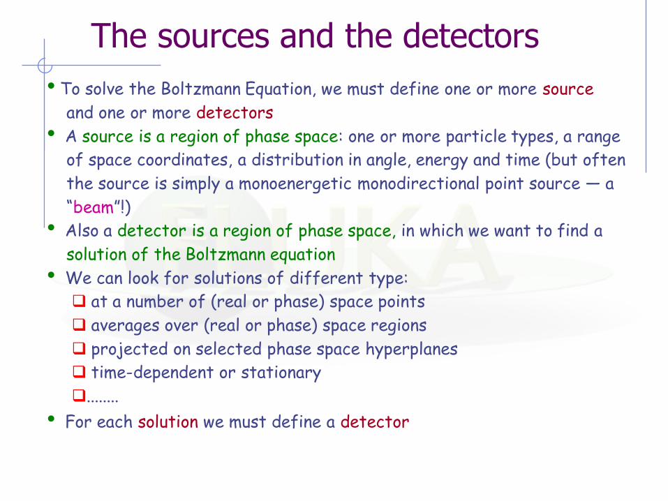
• To solve the Boltzmann Equation, we must define one or more source

and one or more detectors

• A source is a region of phase space: one or more particle types, a range

of space coordinates, a distribution in angle, energy and time (but often

the source is simply a monoenergetic monodirectional point source ― a

“beam”!)

• Also a detector is a region of phase space, in which we want to find a

solution of the Boltzmann equation

• We can look for solutions of different type:

at a number of (real or phase) space points

averages over (real or phase) space regions

projected on selected phase space hyperplanes

time-dependent or stationary

........

• For each solution we must define a detector

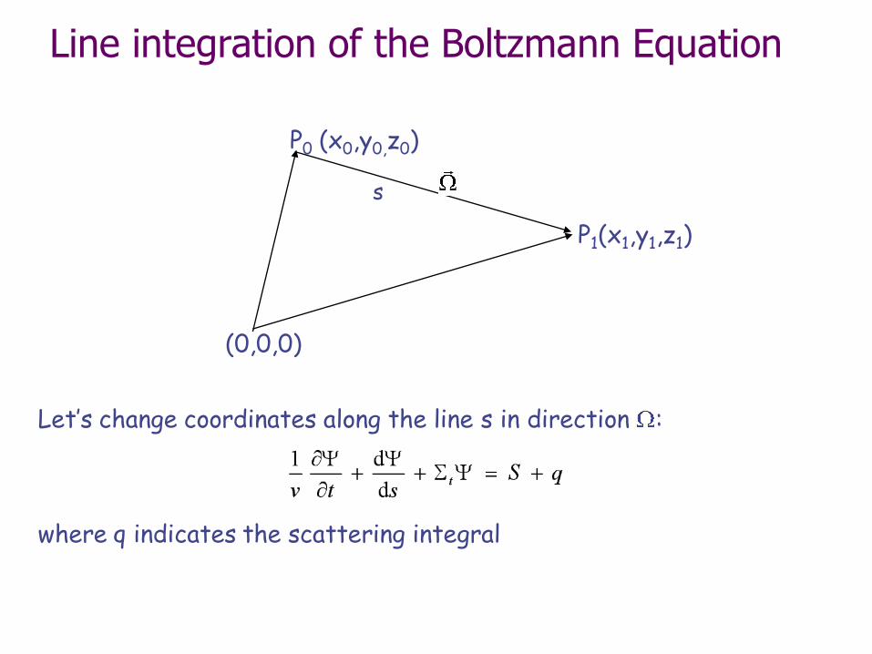
Line integration of the Boltzmann Equation

Let’s change coordinates along the line s in direction :

where q indicates the scattering integral

1r

s

P1(x1,y1,z1)

(0,0,0)

P0 (x0,y0,z0)

s

“source” and “detector” are two regions of phase space

From source to detector without interaction

source S

detector = 0

uncollided term 0

= optical thickness

e- = probability to reach detector without absorption nor scattering

E,

source S

detector

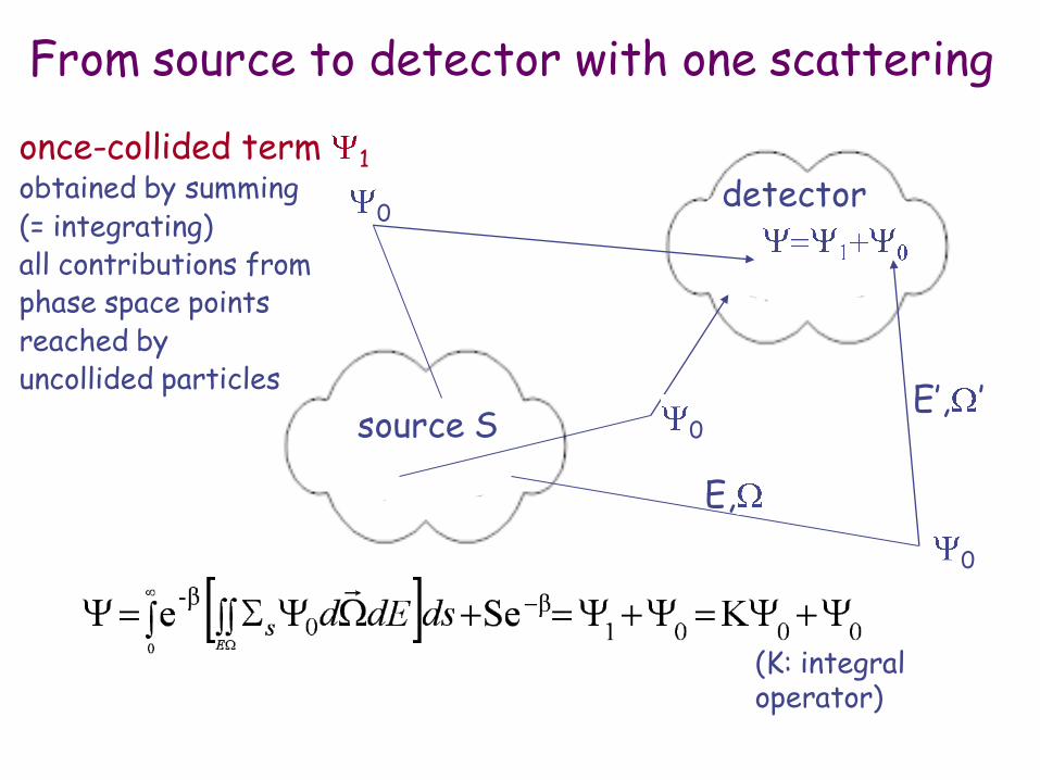
From source to detector with one scattering

once-collided term 1 obtained by summing (= integrating) all contributions from phase space points reached by uncollided particles

E,

E’, ’

(K: integral operator)

0

0

0

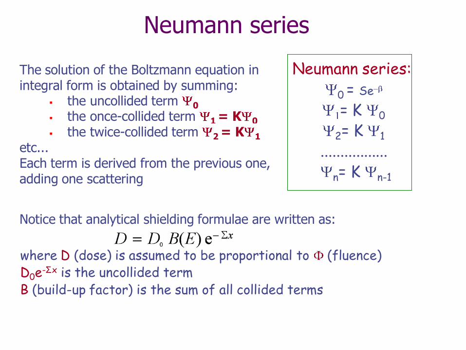
Neumann series

The solution of the Boltzmann equation in integral form is obtained by summing:

the uncollided term 0

the once-collided term 1 = K 0

the twice-collided term 2 = K 1

etc... Each term is derived from the previous one, adding one scattering Notice that analytical shielding formulae are written as: where D (dose) is assumed to be proportional to (fluence) D0e-Σx is the uncollided term B (build-up factor) is the sum of all collided terms

Neumann series:

0 = Se

= K 0

2= K 1 ................. n= K n-1

Integration efficiency • Traditional numerical integration methods (e.g., Simpson) converge to the true

value as N-1/n, where N = number of “points” (intervals) and n = number of

dimensions

• Monte Carlo converges as N-1/2, independent of the number of dimensions

• Therefore:

n = 1 MC is not convenient

n = 2 MC is about equivalent to traditional methods

n > 2 MC converges faster (and the more so the greater the dimensions)

• With the integro-differential Boltzmann equation the dimensions are the 7 of

phase space, but we use the integral form: the dimensions are those of the

largest number of “collisions” per history (the Neumann term of highest order)

• Note that the term “collision” comes from low-energy neutron/photon transport

theory. Here it should be understood in the extended meaning of “interaction

where the particle changes its direction and/or energy, or produces new particles”

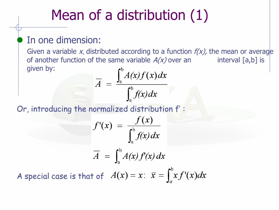
Mean of a distribution (1)

In one dimension: Given a variable x, distributed according to a function f(x), the mean or average

of another function of the same variable A(x) over an interval [a,b] is given by:

Or, introducing the normalized distribution f’ :

A special case is that of

Mean of a distribution (2)

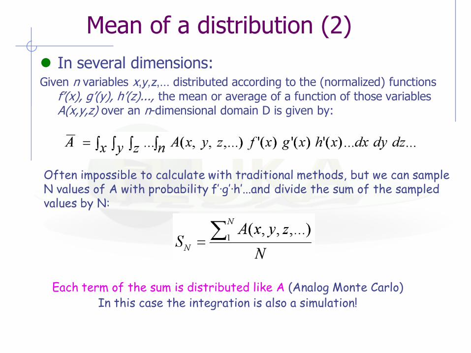
In several dimensions: Given n variables x,y,z,... distributed according to the (normalized) functions

f’(x), g’(y), h’(z)..., the mean or average of a function of those variables A(x,y,z) over an n-dimensional domain D is given by:

Often impossible to calculate with traditional methods, but we can sample N values of A with probability f’·g’·h’...and divide the sum of the sampled values by N:

Each term of the sum is distributed like A (Analog Monte Carlo) In this case the integration is also a simulation!

Central Limit theorem

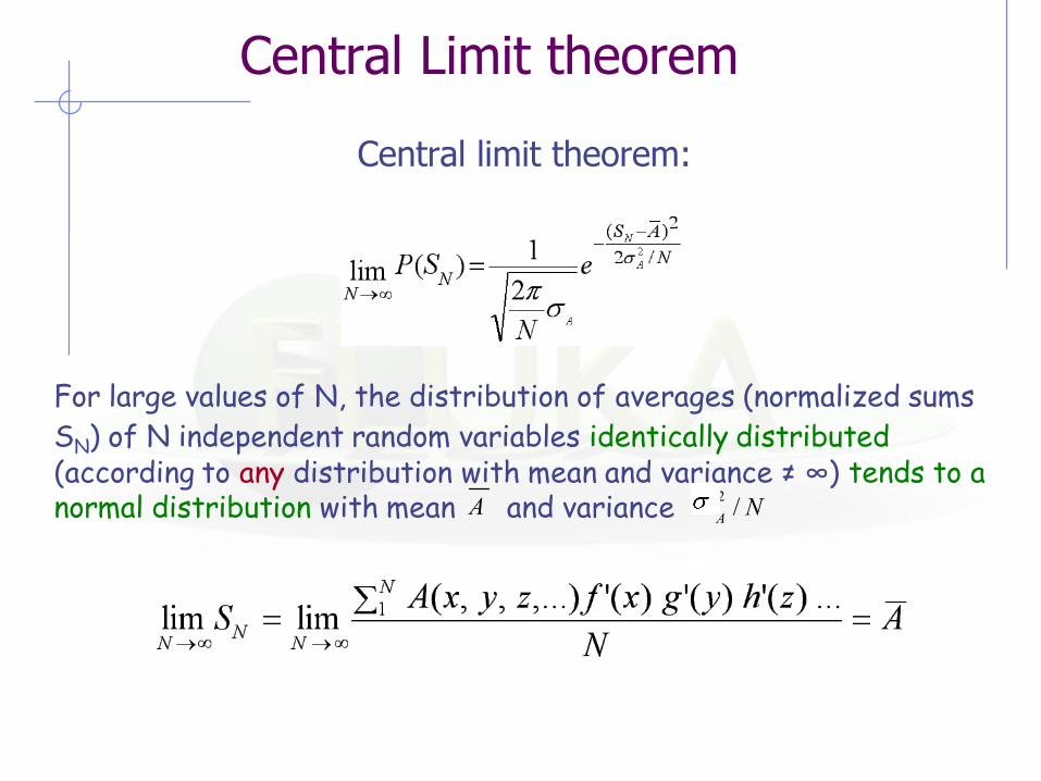
Central limit theorem:

For large values of N, the distribution of averages (normalized sums

SN) of N independent random variables identically distributed (according to any distribution with mean and variance ≠ ∞) tends to a normal distribution with mean and variance A N

A/

2

MC Mathematical foundation

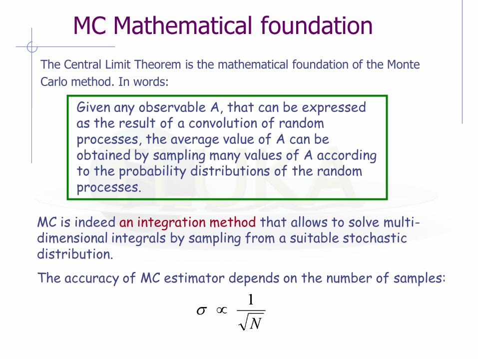
The Central Limit Theorem is the mathematical foundation of the Monte

Carlo method. In words:

Given any observable A, that can be expressed as the result of a convolution of random processes, the average value of A can be obtained by sampling many values of A according to the probability distributions of the random processes.

MC is indeed an integration method that allows to solve multi-dimensional integrals by sampling from a suitable stochastic distribution.

The accuracy of MC estimator depends on the number of samples:

Integration? Or simulation?

Why, then, is MC often considered a simulation

technique?

• Originally, the Monte Carlo method was not a

simulation method, but a device to solve a

multidimensional integro-differential equation by

building a stochastic process such that some

parameters of the resulting distributions would

satisfy that equation

• The equation itself did not necessarily refer to a

physical process, and if it did, that process was not

necessarily stochastic

The Monte Carlo method

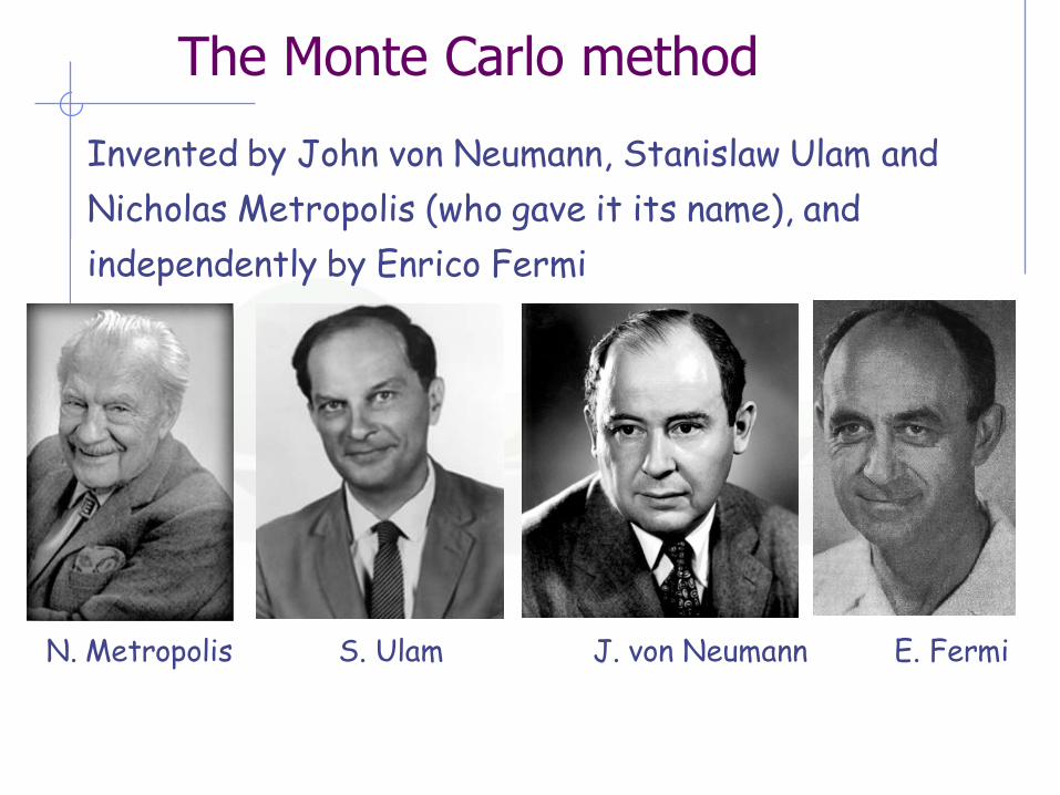
Invented by John von Neumann, Stanislaw Ulam and

Nicholas Metropolis (who gave it its name), and

independently by Enrico Fermi

N. Metropolis S. Ulam J. von Neumann E. Fermi

The ENIAC Electronic Numerical Integrator And Computer

Simulation: in special cases

• It was soon realized, however, that when the

method was applied to an equation describing a

physical stochastic process, such as neutron

diffusion, the model (in this case a random walk)

could be identified with the process itself

• In these cases the method (analog Monte Carlo)

has become known as a simulation technique,

since every step of the model corresponds to an

identical step in the simulated process

Particle transport Particle transport is a typical physical process described by

probabilities (cross sections = interaction probabilities per unit distance)

Therefore it lends itself naturally to be simulated by Monte Carlo

Many applications, especially in high energy physics and medicine, are based on simulations where the history of each particle (trajectory, interactions) is reproduced in detail

However in other types of application, typically shielding design, the user is interested only in the expectation values of some quantities (fluence and dose) at some space point or region, which are calculated as solutions of a mathematical equation

This equation (the Boltzmann equation), describes the statistical distribution of particles in phase space and therefore does indeed represent a physical stochastic process

But in order to estimate the desired expectation values it is not necessary that the Monte Carlo process be identical to it

Integration without simulation

In many cases, it is more efficient to replace the actual process by a different one resulting in the same average values but built by sampling from modified distributions

Such a biased process, if based on mathematically correct variance reduction techniques, converges to the same expectation values as the unbiased one

But it cannot provide information about the higher moments of statistical distributions (fluctuations and correlations)

In addition, the faster convergence in some user-privileged regions of phase space is compensated by a slower convergence elsewhere

Analog Monte Carlo

In an analog Monte Carlo calculation, not only the mean of the contributions converges to the mean of the actual distribution, but also the variance and all moments of higher order:

Then, partial distributions, fluctuations and correlations are all faithfully reproduced: in this case (and in this case only!) we have a

real simulation

Random sampling: the key to Monte Carlo

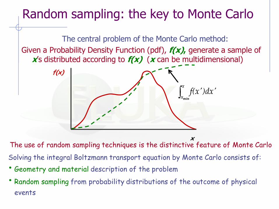
The central problem of the Monte Carlo method:

Given a Probability Density Function (pdf), f(x), generate a sample of x’s distributed according to f(x) (x can be multidimensional)

The use of random sampling techniques is the distinctive feature of Monte Carlo

Solving the integral Boltzmann transport equation by Monte Carlo consists of:

• Geometry and material description of the problem

• Random sampling from probability distributions of the outcome of physical

events

f(x)

x

(Pseudo)random numbers

The basis of all Monte Carlo integrations are random numbers, i.e. random values of a variable distributed according to a pdf

In real world: the random outcomes of physical processes

In computer world: pseudo-random numbers

The basic pdf is the uniform distribution:

• Pseudo-random numbers (PRN) are sequences that reproduce the

uniform distribution, constructed from mathematical algorithms

(PRN generators).

• A PRN sequence looks random but it is not: it can be successfully

tested for statistical randomness although it is generated

deterministically

• A pseudo-random process is easier to produce than a really random

one, and has the advantage that it can be reproduced exactly

• PRN generators have a period, after which the sequence is identically

repeated. However, a repeated number does not imply that the end of

the period has been reached. Some available generators have

periods >1061

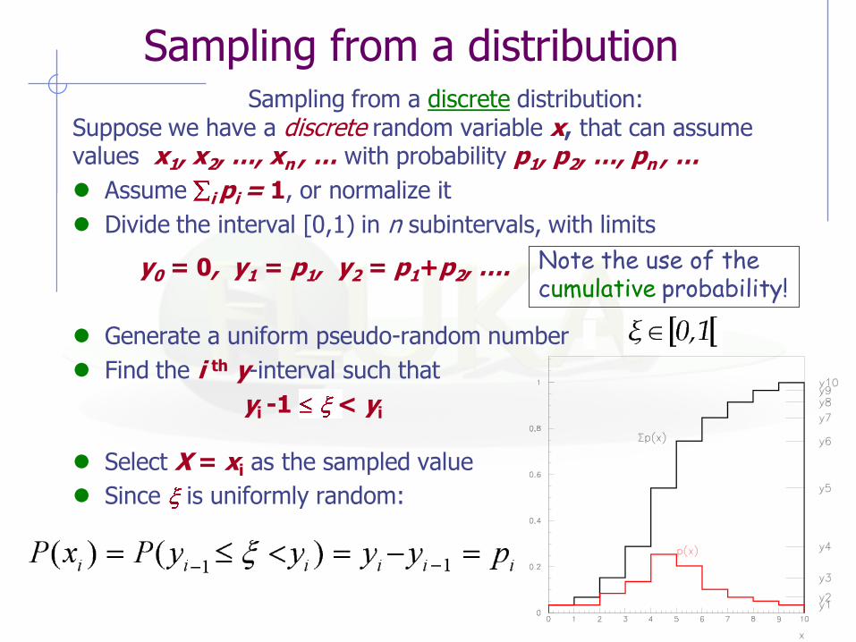
Sampling from a distribution Sampling from a discrete distribution:

Suppose we have a discrete random variable x, that can assume values x1, x2, …, xn , … with probability p1, p2, …, pn , …

Assume i pi = 1, or normalize it

Divide the interval [0,1) in n subintervals, with limits

y0 = 0, y1 = p1, y2 = p1+p2, ….

Generate a uniform pseudo-random number

Find the i th y-interval such that

yi -1 < yi

Select X = xi as the sampled value

Since is uniformly random:

Note the use of the cumulative probability!

Sampling from a distribution

Example: simulate a throw of dice:

x1 = 2, x2 = 3, x3 = 4, ..., x11 = 12 y0 = 0, y1 = 1, y2 = 1+2 = 3, y3 = 3+4 = 7, ..., y11 = 35+1 = 36

Normalize: y0 = 0, y1 = 1/36 = 0.028, y2 = 3/36 = 0.083, y3 = 0.194, ..., y11 = 1

Get a pseudorandom number , e.g.: 0.125

is found to be between y2 = 0.083 and y3 = 0.194

So, our sampled dice throw is x3 = 4

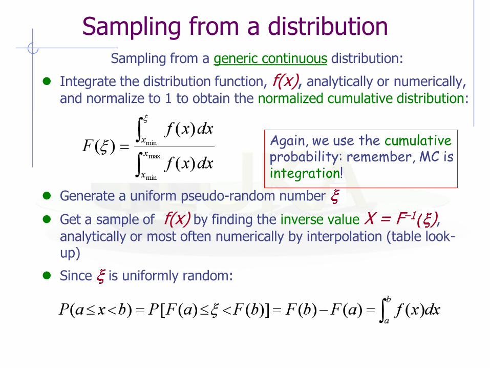
Sampling from a distribution Sampling from a generic continuous distribution:

Integrate the distribution function, f(x), analytically or numerically,

and normalize to 1 to obtain the normalized cumulative distribution:

Generate a uniform pseudo-random number

Get a sample of f(x) by finding the inverse value X = F–1( ), analytically or most often numerically by interpolation (table look-up)

Since is uniformly random:

Again, we use the cumulative probability: remember, MC is integration!

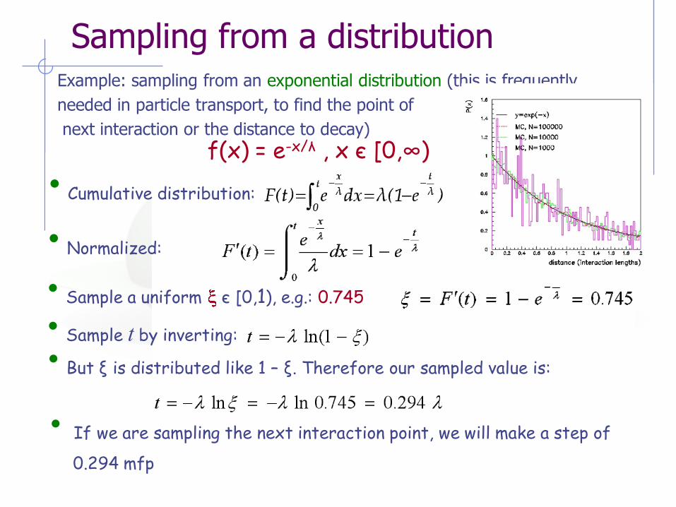
Sampling from a distribution Example: sampling from an exponential distribution (this is frequently

needed in particle transport, to find the point of

next interaction or the distance to decay)

• Cumulative distribution:

• Normalized:

• Sample a uniform є [0,1), e.g.: 0.745

• Sample t by inverting:

• But ξ is distributed like 1 – ξ. Therefore our sampled value is:

• If we are sampling the next interaction point, we will make a step of

0.294 mfp

f(x) = e-x/λ , x є [0,∞)

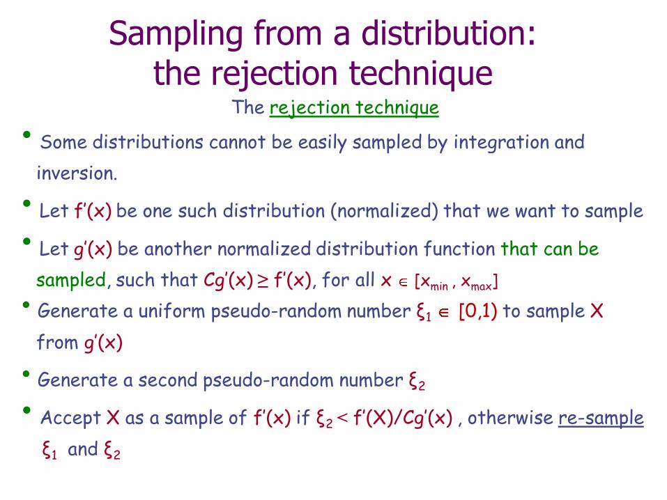
Sampling from a distribution: the rejection technique

The rejection technique

• Some distributions cannot be easily sampled by integration and

inversion.

• Let f’(x) be one such distribution (normalized) that we want to sample

• Let g’(x) be another normalized distribution function that can be

sampled, such that Cg’(x) ≥ f’(x), for all x [xmin , xmax]

• Generate a uniform pseudo-random number ξ1 [0,1) to sample X

from g’(x)

• Generate a second pseudo-random number ξ2

• Accept X as a sample of f’(x) if ξ2 < f’(X)/Cg’(x) , otherwise re-sample

ξ1 and ξ2

Sampling with the rejection technique

• The probability of X to be sampled from g’(x) is g’(X), the one that ξ2 passes the test is f’(X)/Cg’(X) : therefore the probability to have X sampled and accepted is the product of probabilities g’(X) f’(X)/Cg’(X) = f’(X)/C

• The overall efficiency (probability accepted/rejected) is given by

f’(x) is normalized

• Proof that the sampling is unbiased (i.e. X is a correct sample from f’(x)): the probability P(X) dx of sampling X is given by:

• g’(X) is generally chosen as a uniform (rectangular) distribution or

a normalized sum of uniform distributions

(a piecewise constant function) f(x)

x

Cg’(x)

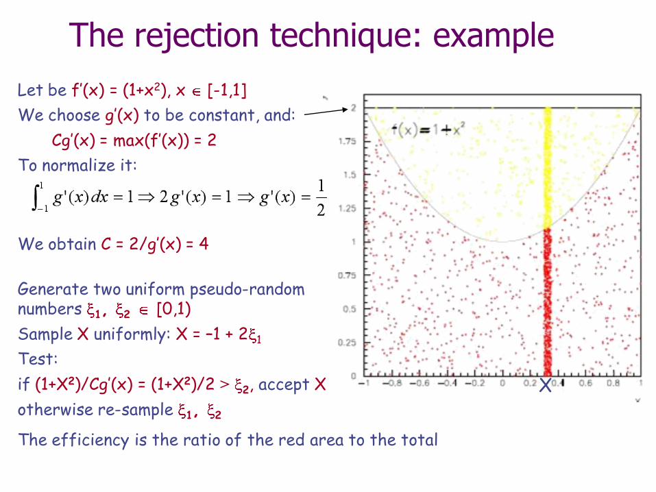
The rejection technique: example

Let be f’(x) = (1+x2), x [-1,1]

We choose g’(x) to be constant, and:

Cg’(x) = max(f’(x)) = 2

To normalize it: We obtain C = 2/g’(x) = 4

Generate two uniform pseudo-random numbers 1, 2 [0,1)

Sample X uniformly: X = –1 + 2 1

Test:

if (1+X2)/Cg’(x) = (1+X2)/2 > 2, accept X

otherwise re-sample 1, 2

X

The efficiency is the ratio of the red area to the total

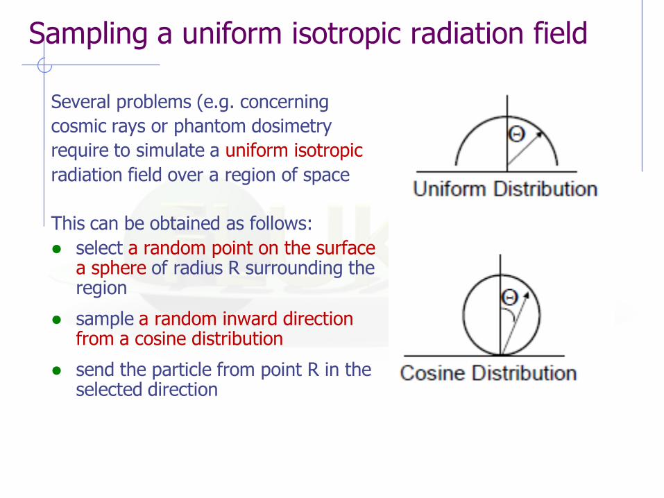
Sampling a uniform isotropic radiation field

Several problems (e.g. concerning

cosmic rays or phantom dosimetry

require to simulate a uniform isotropic

radiation field over a region of space

This can be obtained as follows:

select a random point on the surface a sphere of radius R surrounding the region

sample a random inward direction from a cosine distribution

send the particle from point R in the selected direction

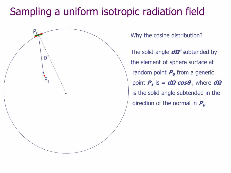
Sampling a uniform isotropic radiation field

Why the cosine distribution?

The solid angle dΩ’ subtended by

the element of sphere surface at

random point P0 from a generic

point P1 is = dΩ cosθ , where dΩ

is the solid angle subtended in the

direction of the normal in P0

θ

P1

P0

•

•

•

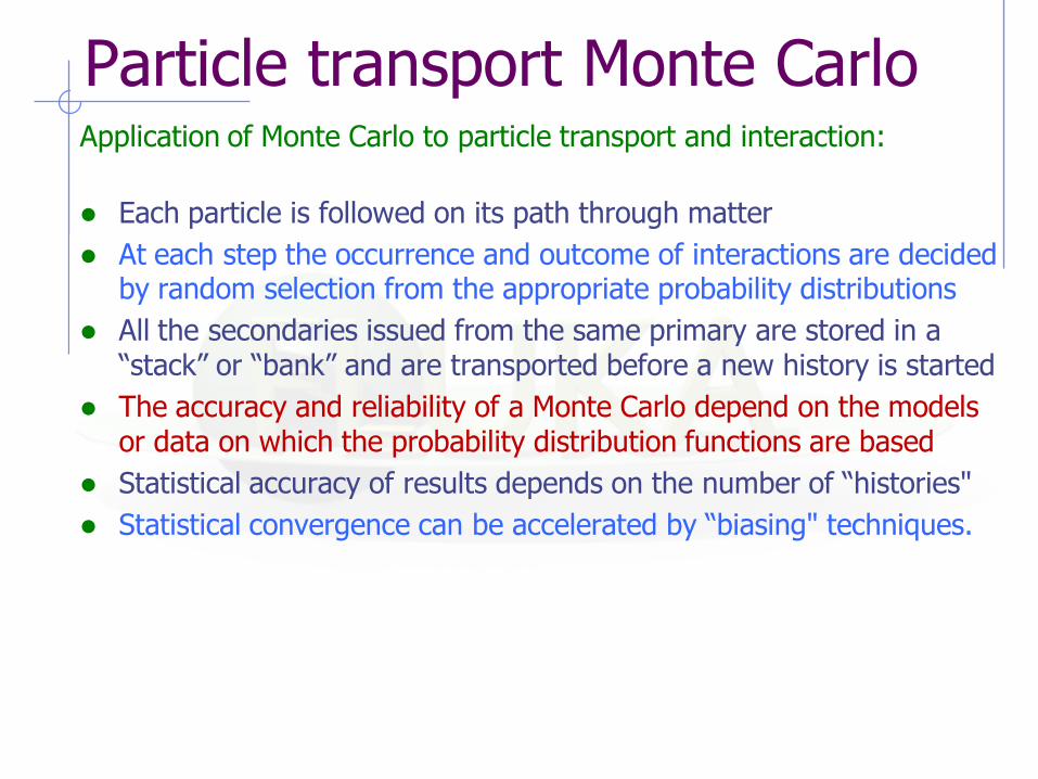
Particle transport Monte Carlo Application of Monte Carlo to particle transport and interaction:

Each particle is followed on its path through matter

At each step the occurrence and outcome of interactions are decided by random selection from the appropriate probability distributions

All the secondaries issued from the same primary are stored in a “stack” or “bank” and are transported before a new history is started

The accuracy and reliability of a Monte Carlo depend on the models or data on which the probability distribution functions are based

Statistical accuracy of results depends on the number of “histories"

Statistical convergence can be accelerated by “biasing" techniques.

Particle transport Monte Carlo Assumptions made by most MC codes: Static, homogeneous, isotropic, amorphous media and geometry Problems: e.g. moving targets*, atmosphere must be represented by

discrete layers of uniform density, radioactive decay may take place in a geometry different from that in which the radionuclides were produced*.

* These restrictions have been overcome in FLUKA

Markovian process: the fate of a particle depends only on its actual present properties, not on previous events or histories

Particles do not interact with each other Problem: e.g. the Chudakov effect (charges cancelling in e+e– pairs)

Particles interact with individual electrons / atoms / nuclei / molecules

Problem: invalid at low energies (X-ray mirrors)

Material properties are not affected by particle reactions Problem: e.g. burnup

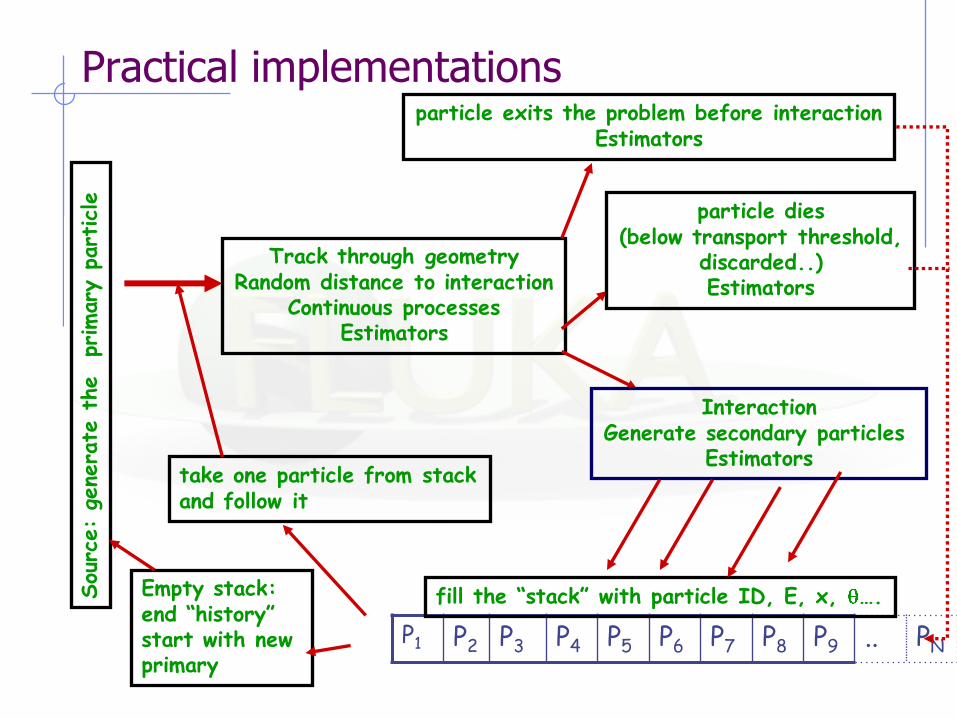
Practical implementations

P1 P2 P3 P4 P5 P6 P7 P8 P9 .. PN

Track through geometry Random distance to interaction

Continuous processes Estimators

particle exits the problem before interaction Estimators

particle dies (below transport threshold,

discarded..) Estimators

Interaction Generate secondary particles

Estimators

fill the “stack” with particle ID, E, x, ….

take one particle from stack and follow it

Empty stack: end “history” start with new primary

Sou

rce:

gene

rate

the

primary

part

icle

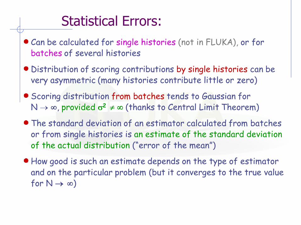
Statistical Errors:

Can be calculated for single histories (not in FLUKA), or for batches of several histories

Distribution of scoring contributions by single histories can be very asymmetric (many histories contribute little or zero)

Scoring distribution from batches tends to Gaussian for N , provided 2 (thanks to Central Limit Theorem)

The standard deviation of an estimator calculated from batches or from single histories is an estimate of the standard deviation of the actual distribution (“error of the mean”)

How good is such an estimate depends on the type of estimator and on the particular problem (but it converges to the true value for N )

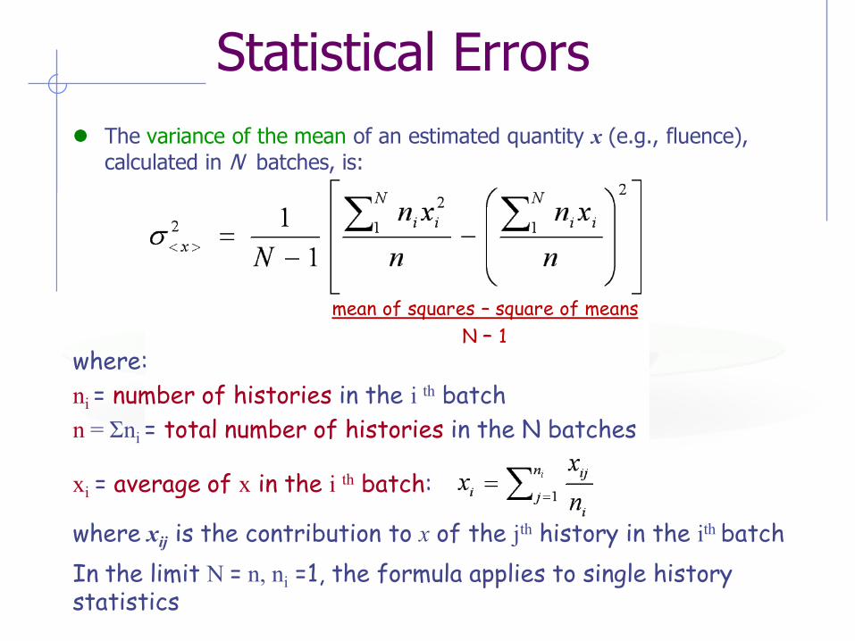
Statistical Errors

The variance of the mean of an estimated quantity x (e.g., fluence),

calculated in N batches, is:

mean of squares – square of means

N – 1

where:

ni = number of histories in the i th batch

n = Σni = total number of histories in the N batches

xi = average of x in the i th batch:

where xij is the contribution to x of the jth history in the ith batch

In the limit N = n, ni =1, the formula applies to single history statistics

Statistical Errors Practical tips:

• Use always at least 5-10 batches of comparable size (it is not at

all mandatory that they be of equal size)

• Never forget that the variance itself is a stochastic variable

subject to fluctuations

• Be careful about the way convergence is achieved: often

(particularly with biasing) apparently good statistics with few

isolated spikes could point to a lack of sampling of the most

relevant phase-space part

• Plot 2D and 3D distributions! In those cases the eye is the best

tool in judging the quality of the result

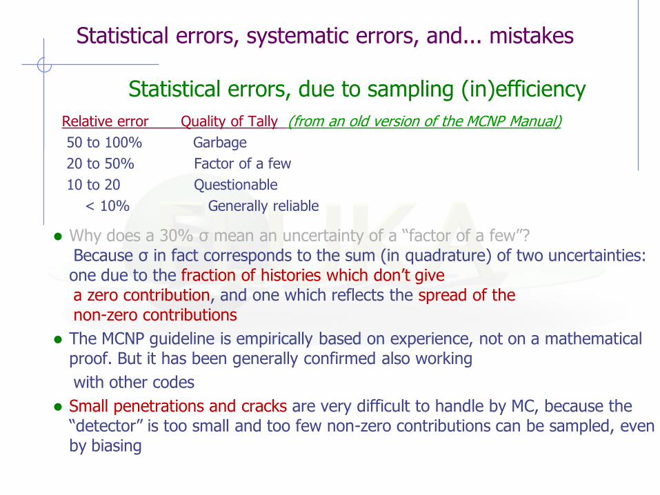
Statistical errors, systematic errors, and... mistakes

Statistical errors, due to sampling (in)efficiency

Relative error Quality of Tally (from an old version of the MCNP Manual)

50 to 100% Garbage

20 to 50% Factor of a few

10 to 20 Questionable

< 10% Generally reliable

Why does a 30% σ mean an uncertainty of a “factor of a few”? Because σ in fact corresponds to the sum (in quadrature) of two uncertainties:

one due to the fraction of histories which don’t give a zero contribution, and one which reflects the spread of the non-zero contributions

The MCNP guideline is empirically based on experience, not on a mathematical proof. But it has been generally confirmed also working

with other codes

Small penetrations and cracks are very difficult to handle by MC, because the “detector” is too small and too few non-zero contributions can be sampled, even by biasing

Statistical errors, systematic errors, and... mistakes

Systematic errors, due to code weaknesses

Apart from the statistical error, which other factors affect the accuracy of MC results?

physics: different codes are based on different physics models. Some models are better than others. Some models are better in a certain energy range. Model quality is best shown by benchmarks at the microscopic level (e.g. thin targets)

artifacts: due to imperfect algorithms, e.g., energy deposited in the middle of a step*, inaccurate path length correction for multiple scattering*, missing correction for cross section and dE/dx change over a step*, etc. Algorithm quality is best shown by benchmarks at the macroscopic level (thick targets, complex geometries)

data uncertainty: an error of 1% in the absorption cross section can lead to an error of a factor 2.8 in the effectiveness of a thick shielding wall (10 attenuation lengths). Results can never be better than allowed by available experimental data!

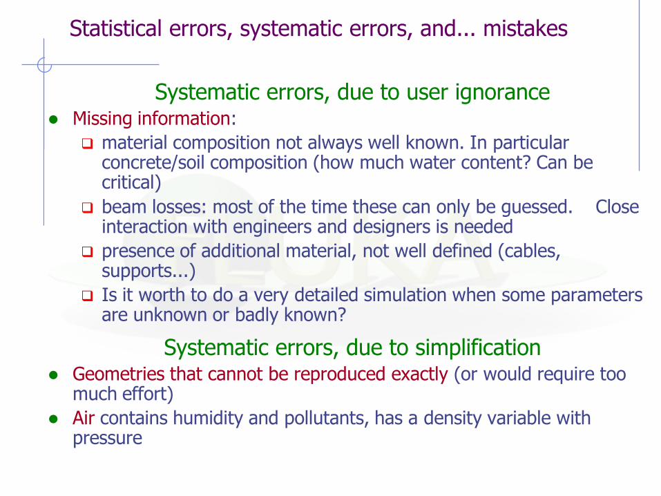
Statistical errors, systematic errors, and... mistakes

Systematic errors, due to user ignorance Missing information:

material composition not always well known. In particular concrete/soil composition (how much water content? Can be critical)

beam losses: most of the time these can only be guessed. Close interaction with engineers and designers is needed

presence of additional material, not well defined (cables, supports...)

Is it worth to do a very detailed simulation when some parameters are unknown or badly known?

Systematic errors, due to simplification Geometries that cannot be reproduced exactly (or would require too

much effort)

Air contains humidity and pollutants, has a density variable with pressure

Statistical errors, systematic errors, and... mistakes

Code mistakes (“bugs”) MC codes can contain bugs:

Physics bugs: I have seen pair production cross sections fitted by a polynomial... and oscillating instead of saturating at high energies, non-uniform azimuthal scattering distributions, energy non-conservation...

Programming bugs (as in any other software, of course)

User mistakes

mis-typing the input: Flair is good at checking, but the final responsibility is the user’s

error in user code: use the built-in features as much as possible!

wrong units

wrong normalization: quite common

unfair biasing: energy/space cuts cannot be avoided, but must be done with much care

forgetting to check that gamma production is available in the neutron cross sections (e.g. Ba cross sections)