Ralf Korn

Compact course

„Monte Carlo Methods for Application

in the Engineering Sciences“

15/16. Mai 2014, Fraunhofer ITWM,

ZV 14.04

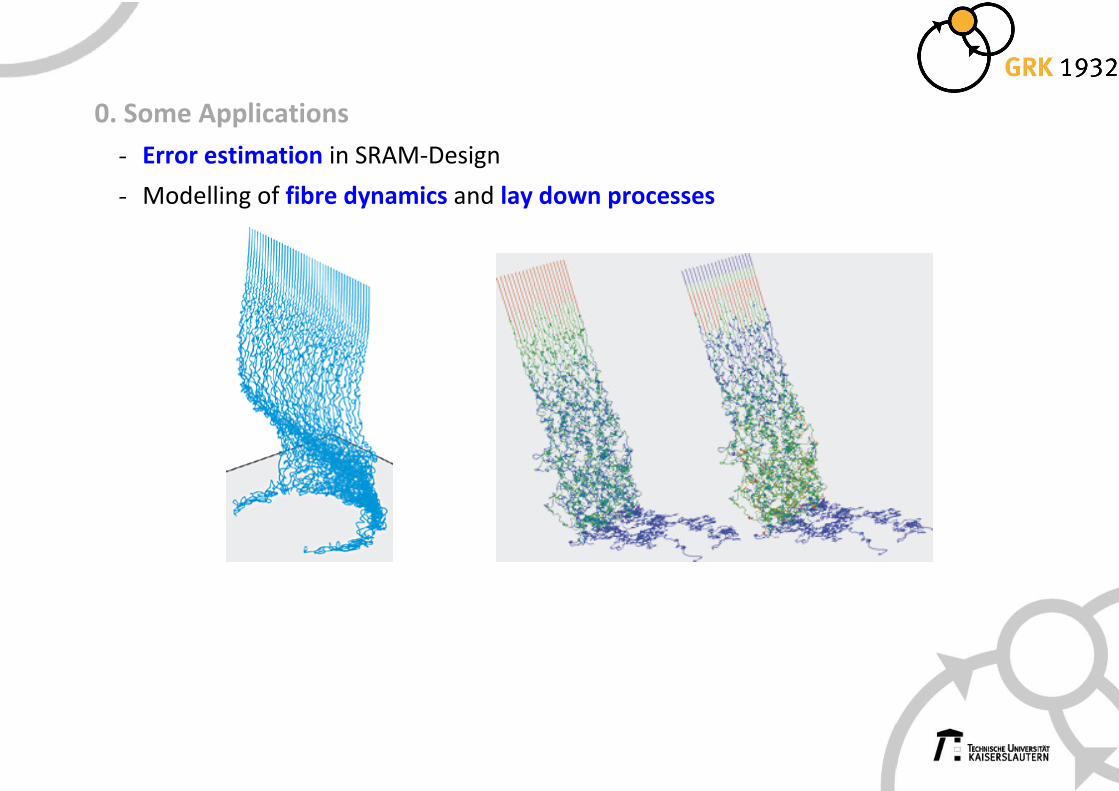
0. Some Applications

- Error estimation in SRAM-Design

6-Transistor-cell in CMOS-technology

0. Some Applications

- Error estimation in SRAM-Design

- Modelling of fibre dynamics and lay down processes

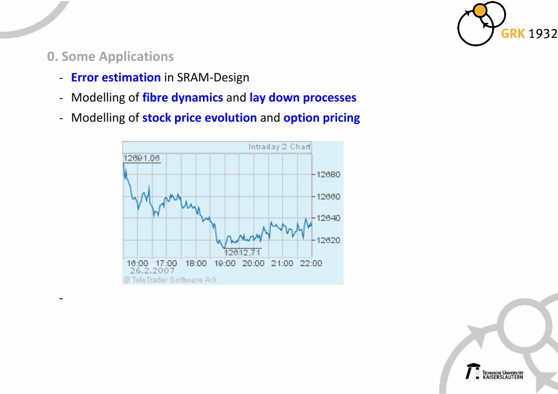
0. Some Applications

- Error estimation in SRAM-Design

- Modelling of fibre dynamics and lay down processes

- Modelling of stock price evolution and option pricing

-

1. Introduction: What is the Monte Carlo method ?

Monte Carlo method = Mathematics (math. algorithm) based on the help of

randomness (?)

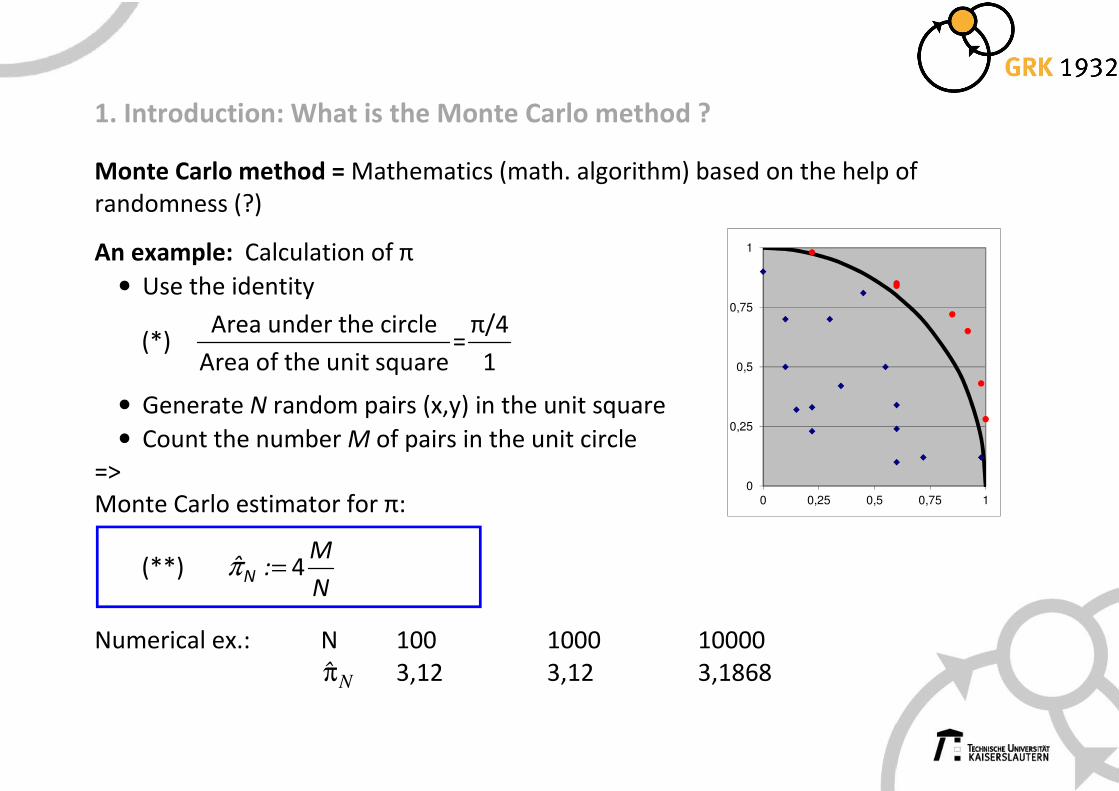
An example: Calculation of π

• Use the identity

(*) Area under the circle π/4

=Area of the unit square 1

• Generate N random pairs (x,y) in the unit square

• Count the number M of pairs in the unit circle

=>

Monte Carlo estimator for π:

(**) =π 4N

Mˆ :

N

Numerical ex.: N 100 1000 10000

Nπ̂ 3,12 3,12 3,1868

0

0,25

0,5

0,75

1

0 0,25 0,5 0,75 1

Generalization of the task:

For a given random variable X with probability distribution P we want to calculate its

mean E(X) (and assume E(X) < ∞).

The strong law of large numbers

Under the above assumptions we have for n independent and identically distributed

(i.i.d.) random numbers xi with probability distribution P:

(1) ( )→∞

=

→∑1

1 nn

i

i

x E Xn

Monte Carlo-Method

• Choose a large number n (i.e. at least 10.000)

• Generate n i.i.d. random numbers xi with probability distribution P

• Estimate E(X) by =

= ∑1

1 n

N i

i

x : xn

Note: The MC-estimator is unbiased and strongly consistent (due to (1)).

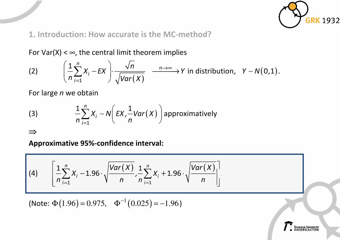
1. Introduction: How accurate is the MC-method?

For Var(X) < ∞, the central limit theorem implies

(2) ( )

( )→∞

=

− ⋅ →

∑ ∼

n

1

1 in distribution 0 1

n

i

i

nX EX Y , Y N ,

n Var X.

For large n we obtain

(3) ( )=

∑ ∼

1

1 1 approximatively

n

i

i

X N EX , Var Xn n

⇒⇒⇒⇒

Approximative 95%-confidence interval:

(4) ( ) ( )

==

− ⋅ ⋅

+∑∑

11

111 96 1 96

n

i

i

n

i

i

Xn

Var X Var XX . , .

n n n.

(Note: ( ) ( )11.96 0.975, 0.025 1.96

−Φ = Φ = − )

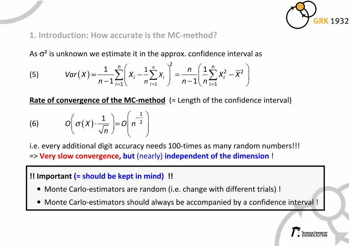
1. Introduction: How accurate is the MC-method?

As σ² is unknown we estimate it in the approx. confidence interval as

(5) ( )== =

≈ − = − − −

∑∑ ∑1

2

2 2

1 1

11 1

1 1

n

i

i

n n

i i

i i

Xn

nVar X X X X

n n n

Rate of convergence of the MC-method (= Length of the confidence interval)

(6) ( )−

⋅ = σ

1

21

O X O nn

i.e. every additional digit accuracy needs 100-times as many random numbers!!!

=> Very slow convergence, but (nearly) independent of the dimension !

!! Important (= should be kept in mind) !!

• Monte Carlo-estimators are random (i.e. change with different trials) !

• Monte Carlo-estimators should always be accompanied by a confidence interval !

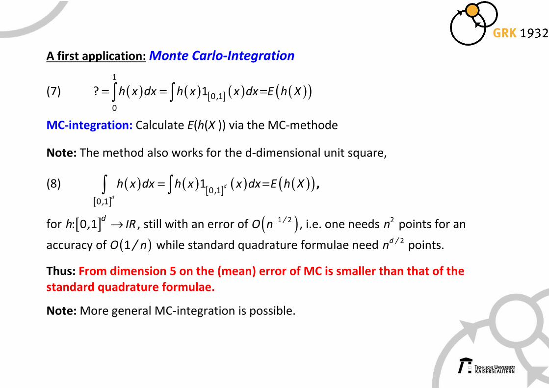
A first application: Monte Carlo-Integration

(7) ( ) ( ) [ ] ( ) ( )( )= = =∫ ∫1

0 1

0

? 1 ,h x dx h x x dx E h X

MC-integration: Calculate E(h(X )) via the MC-methode

Note: The method also works for the d-dimensional unit square,

(8) ( ) ( ) [ ] ( )[ ]

( )( )= =∫ ∫ 0 1

0 1

1 d

d,

,

h x dx h x x dx E h X ,

for [ ] →: 0 1d

h , IR , still with an error of ( )1 2/O n

− , i.e. one needs 2n points for an

accuracy of ( )1O / n while standard quadrature formulae need 2d /n points.

Thus: From dimension 5 on the (mean) error of MC is smaller than that of the

standard quadrature formulae.

Note: More general MC-integration is possible.

A second application: Calculation of probabilities

Aim: Calculate the probability of an event A

⇒

Monte Carlo method

(9) ( )P A = ( ) ( )=

= ≈ ∑1

11 1

i

N

A A

i

P A EN

,

where 1 2iA ,i , ,...,N= denotes the appearance of A in the i. independent replication

of the corresponding experiment

i.e. estimate probabilities by relative frequencies of the occurrence of the event in

repeated experiments.

Next aims:

• Speed up Monte Carlo

o Standard method: variance reduction

o Parallelization and hardware optimization => P2

• How to get all the desired random numbers?

• How to use Monte Carlo for projects P1, 3, 4?

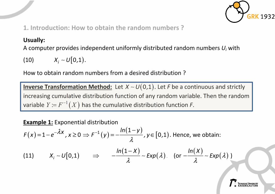
1. Introduction: How to obtain the random numbers ?

Usually:

A computer provides independent uniformly distributed random numbers Ui with

(10) [ )∼ 0 1iX U , .

How to obtain random numbers from a desired distribution ?

Inverse Transformation Method: Let ( )∼ 0 1X U , . Let F be a continuous and strictly

increasing cumulative distribution function of any random variable. Then the random

variable ( )1:Y F X

−= has the cumulative distribution function F.

Example 1: Exponential distribution

( ) −= − ≥λ1 0xF x e , x ⇒ ( )

( )[ )− −

= − ∈λ

1 10 1

ln yF y , y , . Hence, we obtain:

(11) [ )∼ 0 1iX U , ⇒ ( )

( )−

− ∼ λλ

1ln XExp . (or

( )( )− ∼ λ

λ

ln XExp )

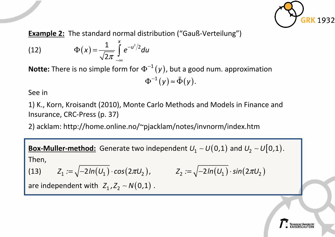
Example 2: The standard normal distribution (“Gauß-Verteilung”)

(12) ( ) −

−∞

Φ = ∫π

2 21

2

xu

x e du

Notte: There is no simple form for ( )−Φ 1y , but a good num. approximation

( ) ( )−Φ ≈ Φɶ1y y .

See in

1) K., Korn, Kroisandt (2010), Monte Carlo Methods and Models in Finance and

Insurance, CRC-Press (p. 37)

2) acklam: http://home.online.no/~pjacklam/notes/invnorm/index.htm

Box-Muller-method: Generate two independent ( )∼1 0 1U U , and [ )∼2 0 1U U , .

Then,

(13) ( ) ( )= − ⋅ π1 1 22 2Z : ln U cos U , ( ) ( )= − ⋅ π2 1 22 2Z : ln U sin U

are independent with ( )∼1 2 0 1Z ,Z N , .

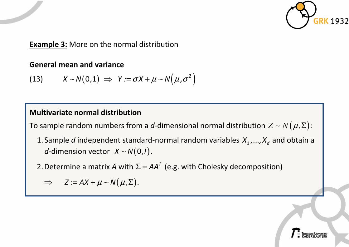
Example 3: More on the normal distribution

General mean and variance

(13) ( )∼ 0 1X N , ⇒ ( )= + ∼σ µ µ σ 2Y : X N ,

Multivariate normal distribution

To sample random numbers from a d-dimensional normal distribution ( ),Z N µ Σ∼ :

1. Sample d independent standard-normal random variables 1 dX ,...,X and obtain a

d-dimension vector ( )∼ 0X N ,I .

2. Determine a matrix A with Σ = TAA (e.g. with Cholesky decomposition)

⇒ ( )= + Σ∼µ µZ : AX N , .

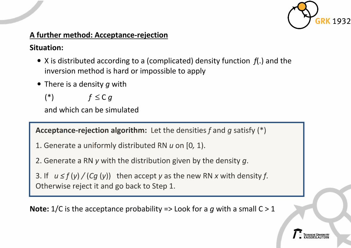
A further method: Acceptance-rejection

Situation:

• X is distributed according to a (complicated) density function f(.) and the

inversion method is hard or impossible to apply

• There is a density g with

(*) f ≤ C g

and which can be simulated

Acceptance-rejection algorithm: Let the densities f and g satisfy (*)

1. Generate a uniformly distributed RN u on [0, 1).

2. Generate a RN y with the distribution given by the density g.

3. If u ≤ f (y) / (Cg (y)) then accept y as the new RN x with density f.

Otherwise reject it and go back to Step 1.

Note: 1/C is the acceptance probability => Look for a g with a small C > 1

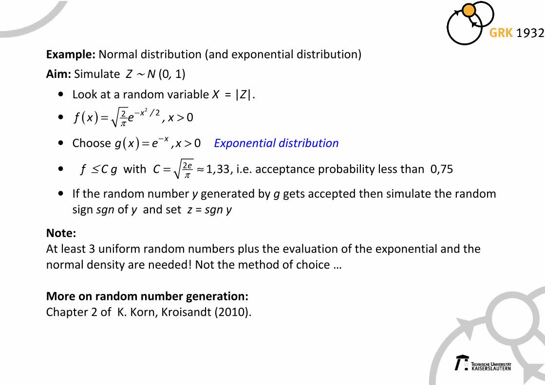
Example: Normal distribution (and exponential distribution)

Aim: Simulate Z ∼ N (0, 1)

• Look at a random variable X = |Z|.

• ( )2 22 0x /

f x e , xπ−= >

• Choose ( ) −= > 0xg x e ,x Exponential distribution

• f ≤ C g with = ≈π2 1 33eC , , i.e. acceptance probability less than 0,75

• If the random number y generated by g gets accepted then simulate the random

sign sgn of y and set z = sgn y

Note:

At least 3 uniform random numbers plus the evaluation of the exponential and the

normal density are needed! Not the method of choice …

More on random number generation:

Chapter 2 of K. Korn, Kroisandt (2010).

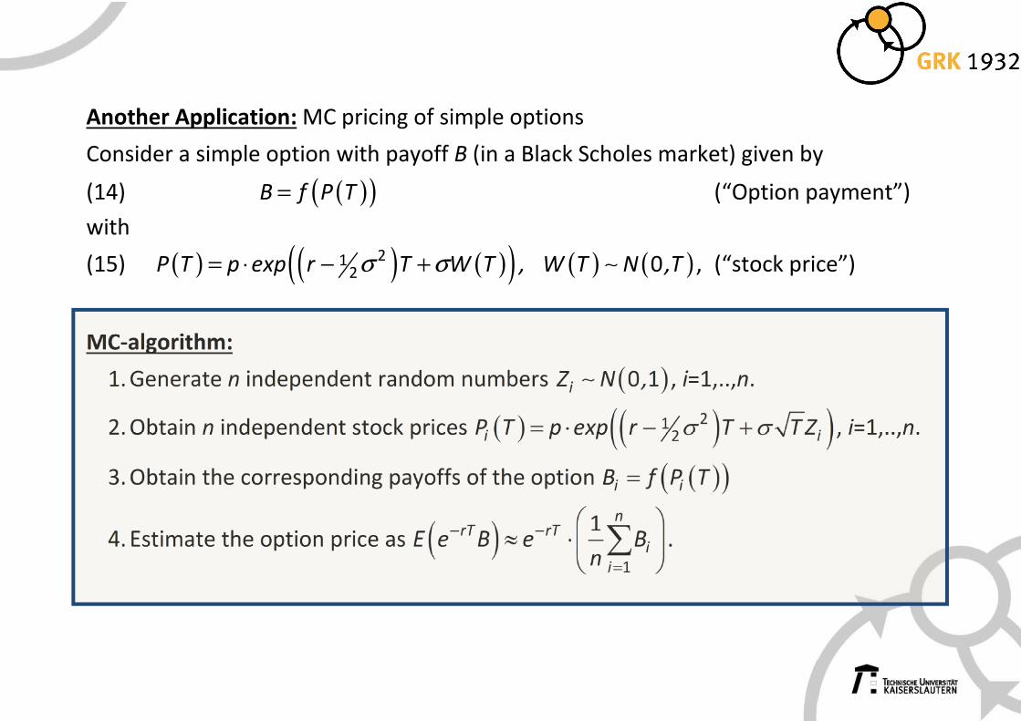
Another Application: MC pricing of simple options

Consider a simple option with payoff B (in a Black Scholes market) given by

(14) ( )( )=B f P T (“Option payment”)

with

(15) ( ) ( ) ( )( ) ( ) ( )= ⋅ − + ∼σ σ212 0P T p exp r T W T , W T N ,T , (“stock price”)

MC-algorithm:

1. Generate n independent random numbers ( )∼ 0 1iZ N , , i=1,..,n.

2. Obtain n independent stock prices ( ) ( )( )= ⋅ − +σ σ212i iP T p exp r T T Z , i=1,..,n.

3. Obtain the corresponding payoffs of the option ( )( )=i iB f P T

4. Estimate the option price as ( )− −

=

≈ ⋅

∑

1

1 nrT rT

i

i

E e B e Bn

.

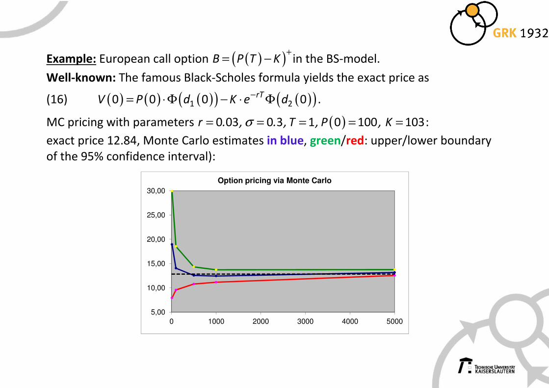
Example: European call option ( )( )+= −B P T K in the BS-model.

Well-known: The famous Black-Scholes formula yields the exact price as

(16) ( ) ( ) ( )( ) ( )( )−= ⋅Φ − ⋅ Φ1 20 0 0 0rTV P d K e d .

MC pricing with parameters ( )= = = = =σ0 03 0 3 1 0 100 103r . , . , T , P , K :

exact price 12.84, Monte Carlo estimates in blue, green/red: upper/lower boundary

of the 95% confidence interval):

5,00

10,00

15,00

20,00

25,00

30,00

0 1000 2000 3000 4000 5000

Option pricing via Monte Carlo

2. Speeding up Monte Carlo via Variance Reduction

Aim: Faster convergence of the method (i.e. less random numbers needed for a

desired precision)

Idea:

• Approximate X by a random variable Y with identical mean, but a smaller

variance.

• Then perform a Monte Carlo calculation for ( )E Y and estimate the

corresponding confidence interval as in (4).

⇒ Shorter confidence interval for the corresponding Monte Carlo-estimator

(“Variance reduction “).

Question: How to do this?

⇒ There are various methods …

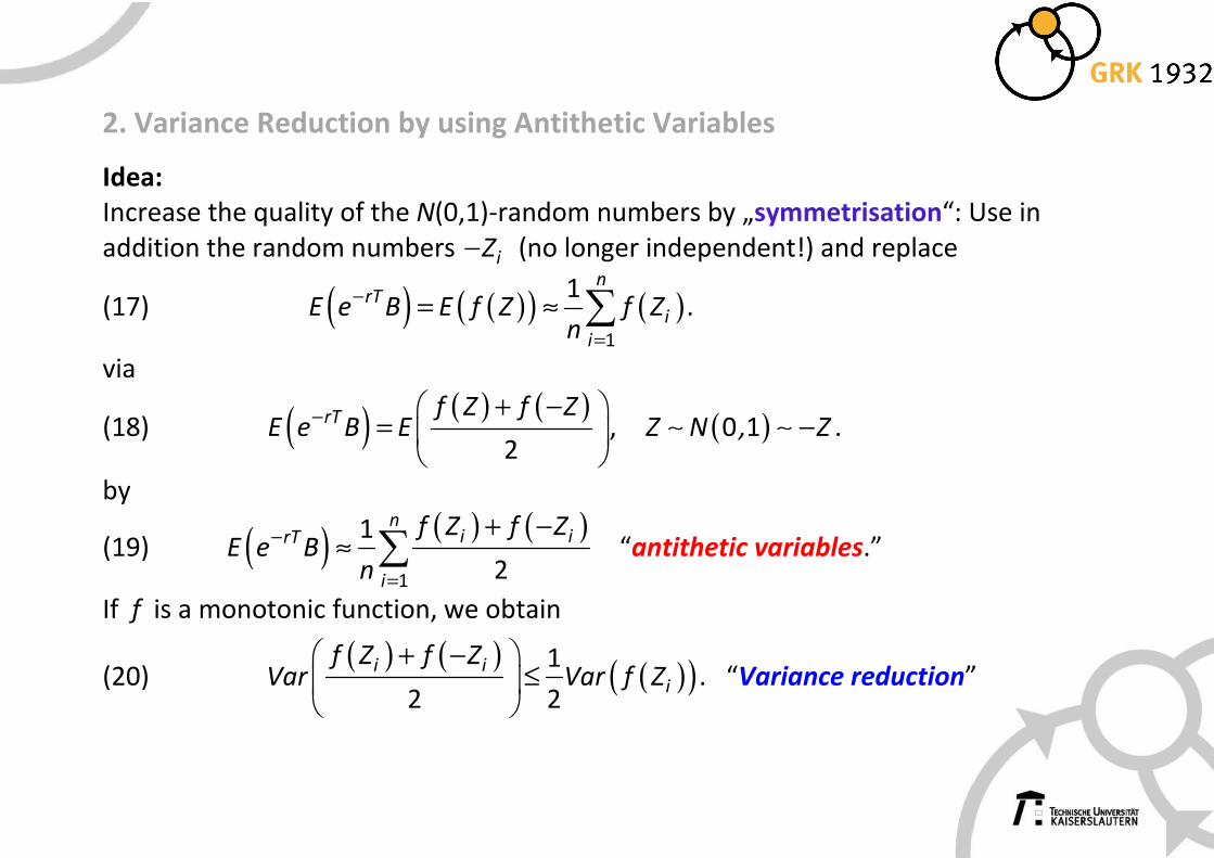
2. Variance Reduction by using Antithetic Variables

Idea:

Increase the quality of the N(0,1)-random numbers by „symmetrisation“: Use in

addition the random numbers − iZ (no longer independent!) and replace

(17) ( ) ( )( ) ( )−

=

= ≈ ∑1

1 nrT

i

i

E e B E f Z f Zn

.

via

(18) ( ) ( ) ( )− + − =

2

rT f Z f ZE e B E , ( ) −∼ ∼0 1Z N , Z .

by

(19) ( ) ( ) ( )−

=

+ −≈ ∑

1

1

2

ni irT

i

f Z f ZE e B

n “antithetic variables.”

If f is a monotonic function, we obtain

(20) ( ) ( )

( )( )+ −

≤

1

2 2

i ii

f Z f ZVar Var f Z . “Variance reduction”

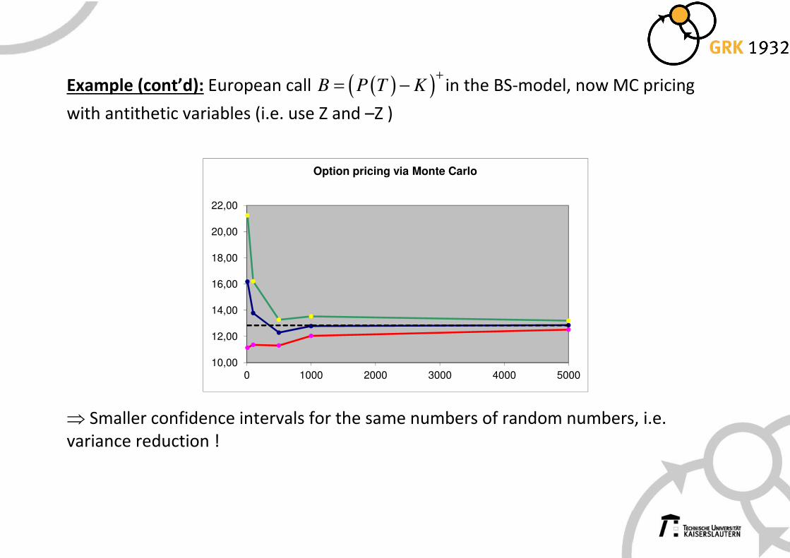
Example (cont’d): European call ( )( )B P T K+

= − in the BS-model, now MC pricing

with antithetic variables (i.e. use Z and –Z )

⇒ Smaller confidence intervals for the same numbers of random numbers, i.e.

variance reduction !

10,00

12,00

14,00

16,00

18,00

20,00

22,00

0 1000 2000 3000 4000 5000

Option pricing via Monte Carlo

2. Variance Reduction by using Control Variates

Goal: Estimate ( )−rTE e B

Known: Explicit pricing formula for another option with payoff ɶB

( )− =ɶrTE e B : F .

⇒

(21) ( ) ( )( )− −= + − ɶrT rTE e B F E e B B .

If ɶB is very similar to B then one hopes for a big variance reduction by using:

(22) ( ) ( ) ( )− −

=

≈ + ⋅ −

∑ ɶ

1

1 nrT rT

i i

i

E e B F e B Bn

.

Theoretical justification:

(23) ( )( ) ( ) ( ) ( )− = + −ɶ ɶ ɶ2Var B B Var B Var B Cov B,B .

Generalising the trick in (22):

(24) ( ) ( )( )rT rTE e B F E e B Bθ θ− −= ⋅ + − ⋅ ɶ ,

suggests

(25) ( ) ( ) ( )1

1 nrT rT

i i

i

E e B F e B Bn

θ θ− −

=

≈ ⋅ + ⋅ − ⋅

∑ ɶ

by choosing the parameter θ to minimize the variance on the right hand side

(26) ( ) ( ) ( ) ( )− = + −ɶ ɶ ɶθ θ θ2 2Var B B Var B Var B Cov B,B .

⇒

(27) ( )( )

=ɶ

ɶθmin

Cov B,B

Var B.

Note:

This value is unknown, but can be estimated during the simulation.

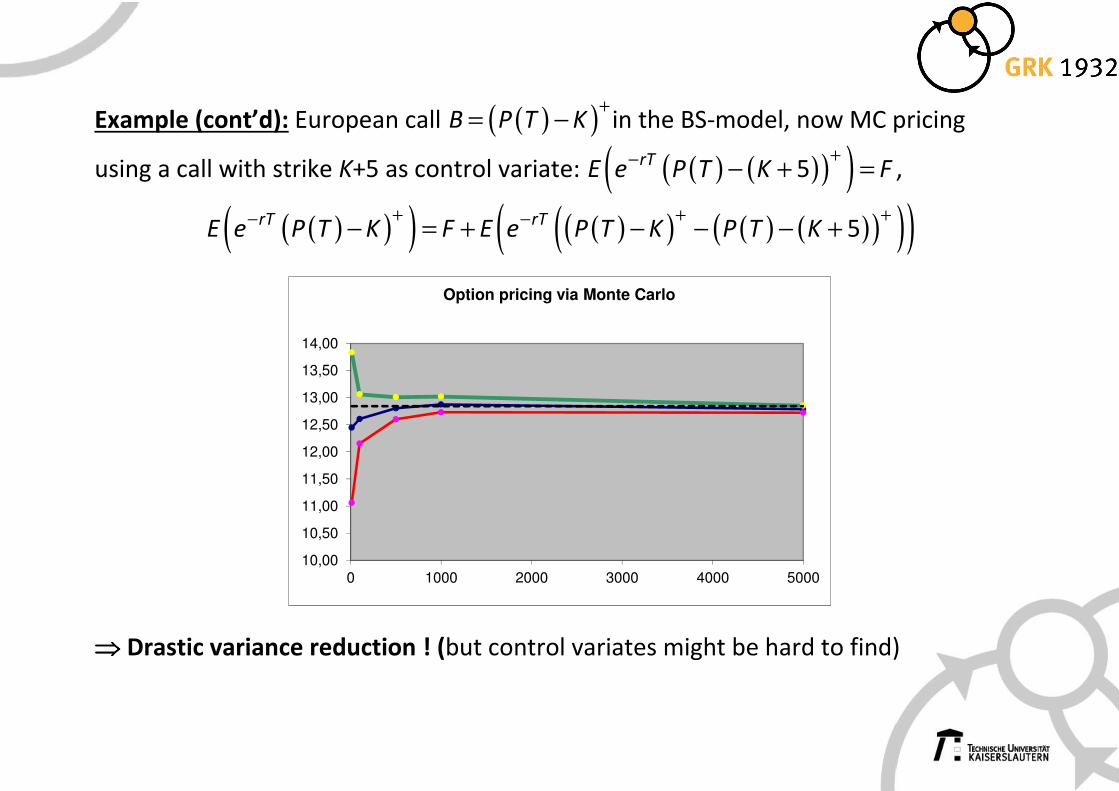
Example (cont’d): European call ( )( )+= −B P T K in the BS-model, now MC pricing

using a call with strike K+5 as control variate: ( ) ( )( )( )+− − + =5rTE e P T K F ,

( )( )( ) ( )( ) ( ) ( )( )( )( )+ + +− −− = + − − − + 5rT rTE e P T K F E e P T K P T K

⇒⇒⇒⇒ Drastic variance reduction ! (but control variates might be hard to find)

10,00

10,50

11,00

11,50

12,00

12,50

13,00

13,50

14,00

0 1000 2000 3000 4000 5000

Option pricing via Monte Carlo

Note: One can combine several methods for improving the Monte Carlo method: e.g.

use both antithetic variables + control variate => even better performance !!!

Other possibilities to improve Monte Carlo methods:

• Multiple Controls

• Importance sampling (=> coming soon !)

• Quasi-Monte Carlo methods

• ......

12,8405

12,8410

12,8415

12,8420

12,8425

12,8430

0 1000 2000 3000 4000 5000

Option pricing via Monte Carlo

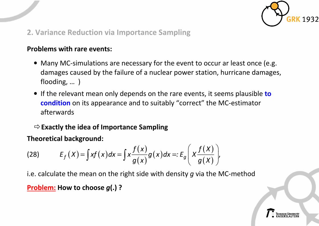
2. Variance Reduction via Importance Sampling

Problems with rare events:

• Many MC-simulations are necessary for the event to occur ar least once (e.g.

damages caused by the failure of a nuclear power station, hurricane damages,

flooding, … )

• If the relevant mean only depends on the rare events, it seems plausible to

condition on its appearance and to suitably “correct” the MC-estimator

afterwards

� Exactly the idea of Importance Sampling

Theoretical background:

(28) ( ) ( )( )( )

( )( )( )

= = =

∫ ∫f g

f x f XE X xf x dx x g x dx : E X

g x g X,

i.e. calculate the mean on the right side with density g via the MC-method

Problem: How to choose g(.) ?

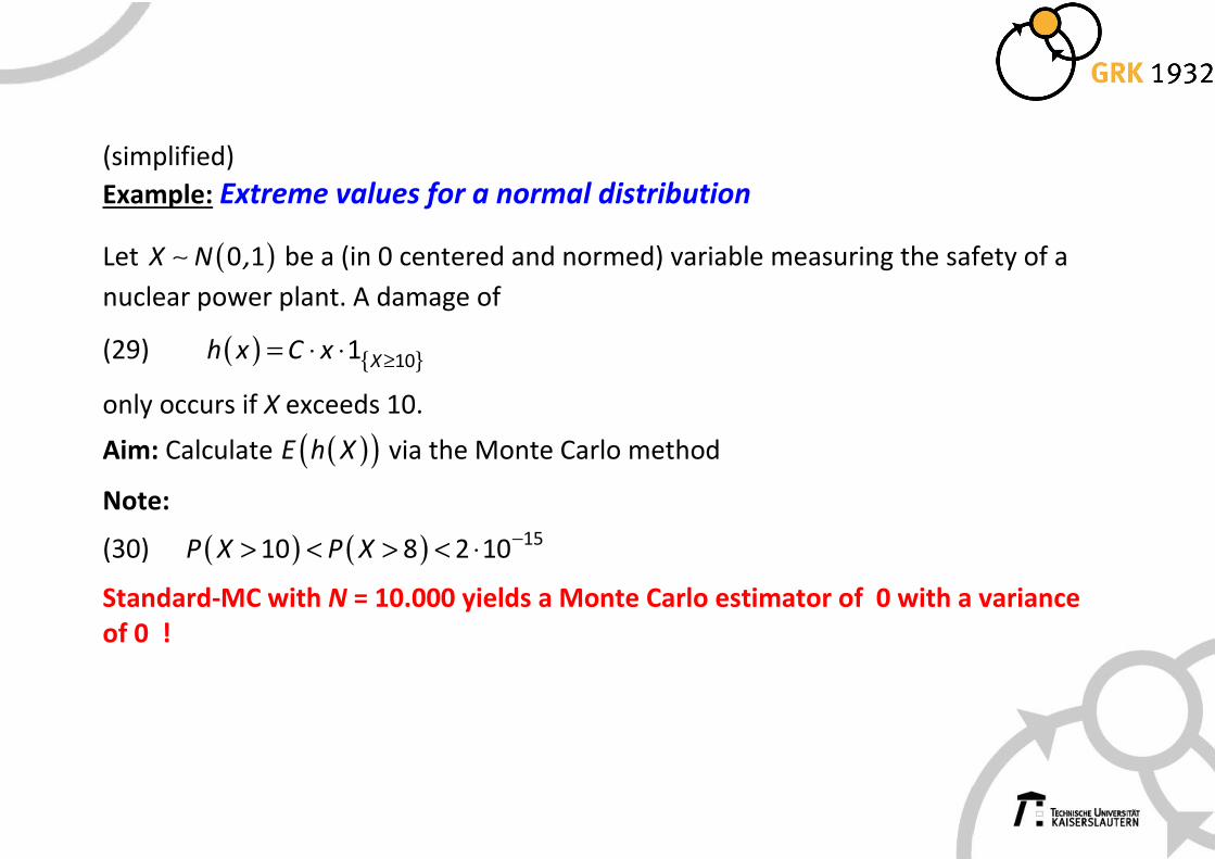
(simplified)

Example: Extreme values for a normal distribution

Let ( )∼ 0 1X N , be a (in 0 centered and normed) variable measuring the safety of a

nuclear power plant. A damage of

(29) ( ) { }≥= ⋅ ⋅ 101 Xh x C x

only occurs if X exceeds 10.

Aim: Calculate ( )( )E h X via the Monte Carlo method

Note:

(30) ( ) ( ) −> < > < ⋅ 1510 8 2 10P X P X

Standard-MC with N = 10.000 yields a Monte Carlo estimator of 0 with a variance

of 0 !

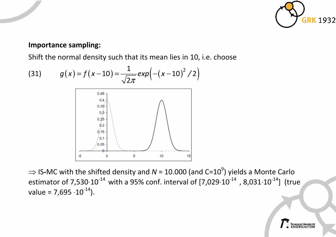
Importance sampling:

Shift the normal density such that its mean lies in 10, i.e. choose

(31) ( ) ( ) ( )( )= − = − −π

2110 10 2

2g x f x exp x /

⇒ IS-MC with the shifted density and N = 10.000 (and C=109) yields a Monte Carlo

estimator of 7,530⋅10-14

with a 95% conf. interval of [7,029⋅10-14

, 8,031⋅10-14

] (true

value = 7,695 ⋅10-14

).

Importance Sampling: Next example

Mixture Importance Sampling and Analysis of SRAM-Design with rare

Failures(Kanj, Joshi, Nassif (2006))

Background:

Continuing miniaturization in chip-design (sub-100nm) leads to an increasing in-

fluence of (stoch.) variability inside the chip on its quality

Particularly for SRAM-cells:

Failure of a few cells can lead to erraneous storage media.

=>

Yield analysis of SRAM-cells is extremely important as small variations in the yield can

lead to high variability of the storage media.

� Exact estimation of the failure rate of SRAM-cells is important

� As the cells are usually „good“, „failure“ is a rare event

� Estimation of the failure rates is a typical application for importance sampling !

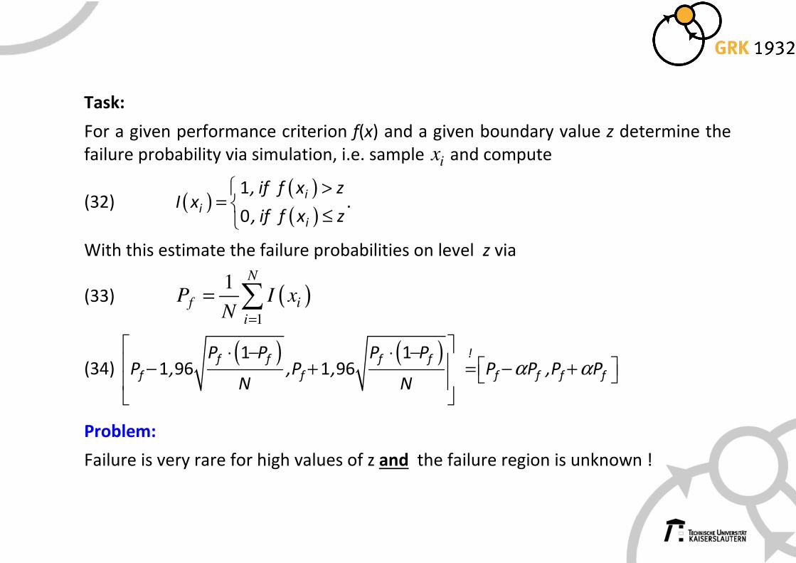
Task:

For a given performance criterion f(x) and a given boundary value z determine the

failure probability via simulation, i.e. sample ix and compute

(32) ( )( )( )

>=

≤

1

0

ii

i

, if f x zI x

, if f x z.

With this estimate the failure probabilities on level z via

(33)

(34) ( ) ( ) ⋅ − ⋅ −

− + = − +

α α1 1

1 96 1 96!f f f f

f f f f f f

P P P PP , ,P , P P ,P P

N N

Problem:

Failure is very rare for high values of z and the failure region is unknown !

( )1

1N

f i

i

P I xN =

= ∑

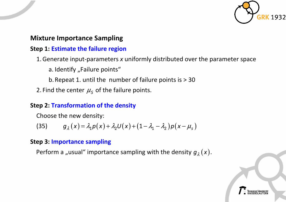
Mixture Importance Sampling

Step 1: Estimate the failure region

1. Generate input-parameters x uniformly distributed over the parameter space

a. Identify „Failure points“

b. Repeat 1. until the number of failure points is > 30

2. Find the center Sµ of the failure points.

Step 2: Transformation of the density

Choose the new density:

(35) ( ) ( ) ( ) ( ) ( )1 2 1 21 sg x p x U x p xλ λ λ λ λ µ= + + − − −

Step 3: Importance sampling

Perform a „usual“ importance sampling with the density ( )g xλ .

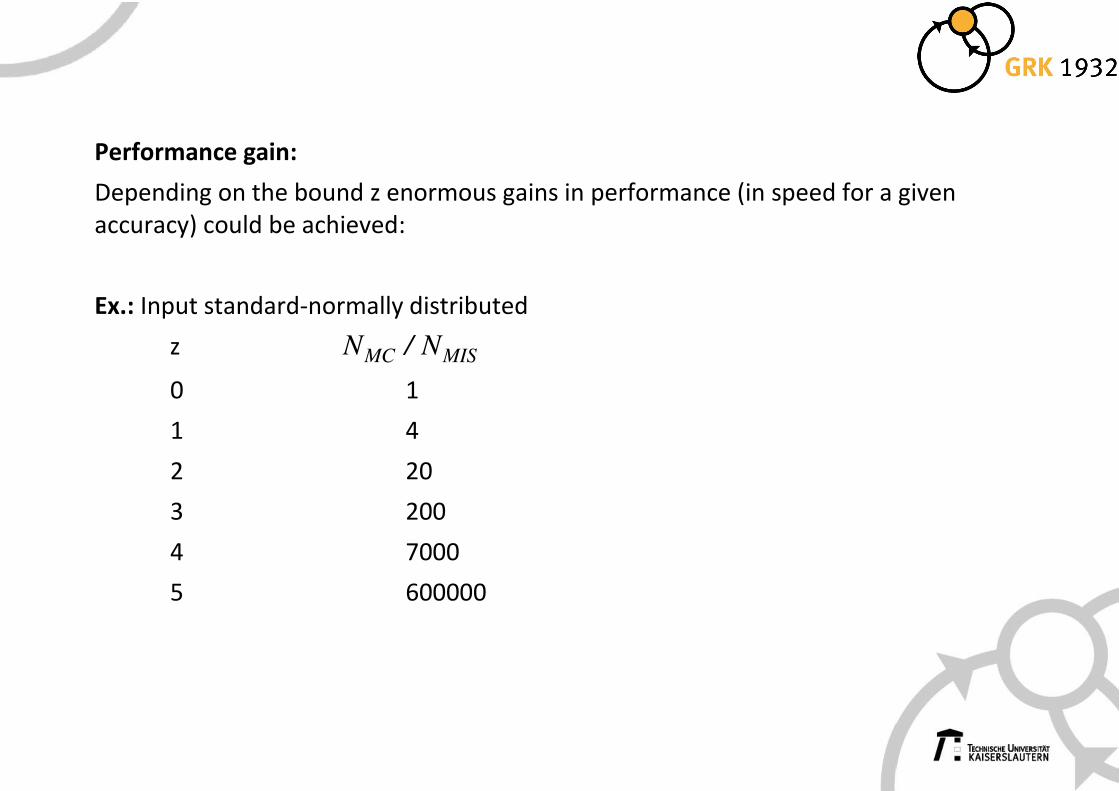
Performance gain:

Depending on the bound z enormous gains in performance (in speed for a given

accuracy) could be achieved:

Ex.: Input standard-normally distributed

z MC MISN / N

0 1

1 4

2 20

3 200

4 7000

5 600000

Literature for Talk 1:

Kanj R., Joshi R., Nassif S. (2006) Mixture importance sampling and its application to

the analysis of SRAM designs in the presence of rare failure events, DAC, 69-72.

Korn E., Korn R., Kroisandt G. (2010) Monte Carlo Methods and Models in Finance and

Insurance. Chapman & Hall, Chapter 3.

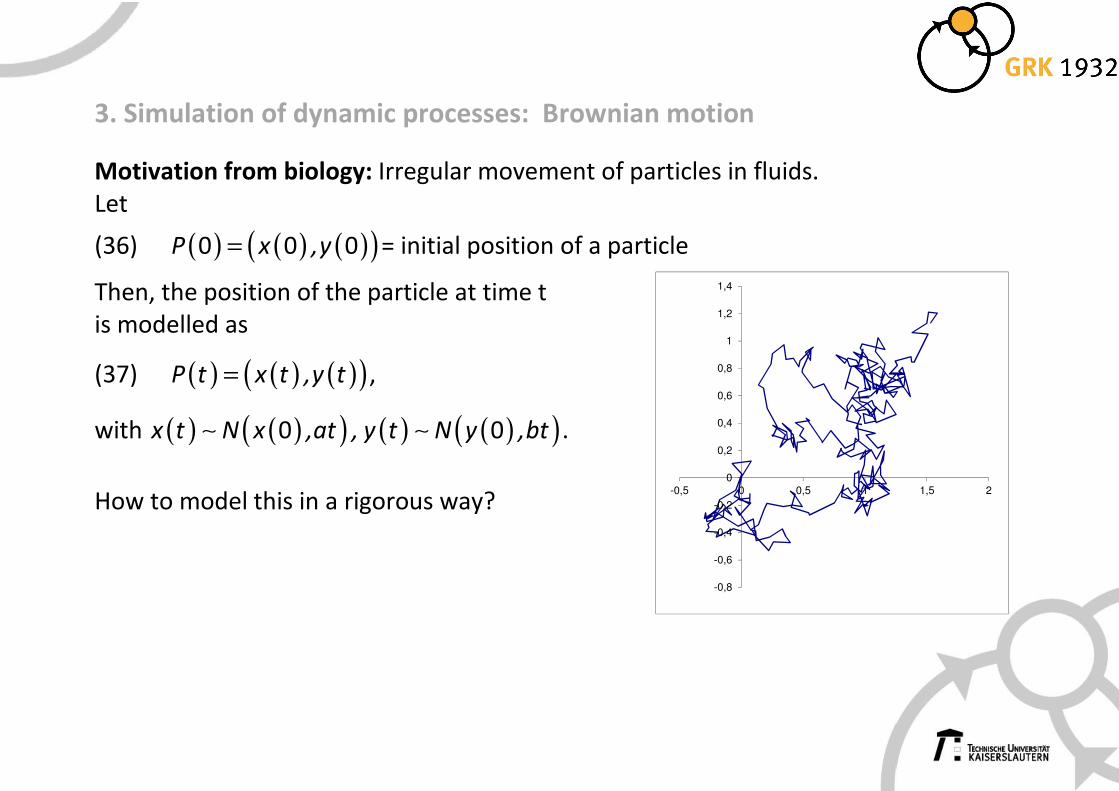
3. Simulation of dynamic processes: Brownian motion

Motivation from biology: Irregular movement of particles in fluids.

Let

(36) ( ) ( ) ( )( )0 0 0P x ,y= = initial position of a particle

Then, the position of the particle at time t

is modelled as

(37) ( ) ( ) ( )( )P t x t ,y t= ,

with ( ) ( )( ) ( ) ( )( )0 0x t N x ,at , y t N y ,bt∼ ∼ .

How to model this in a rigorous way?

-0,8

-0,6

-0,4

-0,2

0

0,2

0,4

0,6

0,8

1

1,2

1,4

-0,5 0 0,5 1 1,5 2

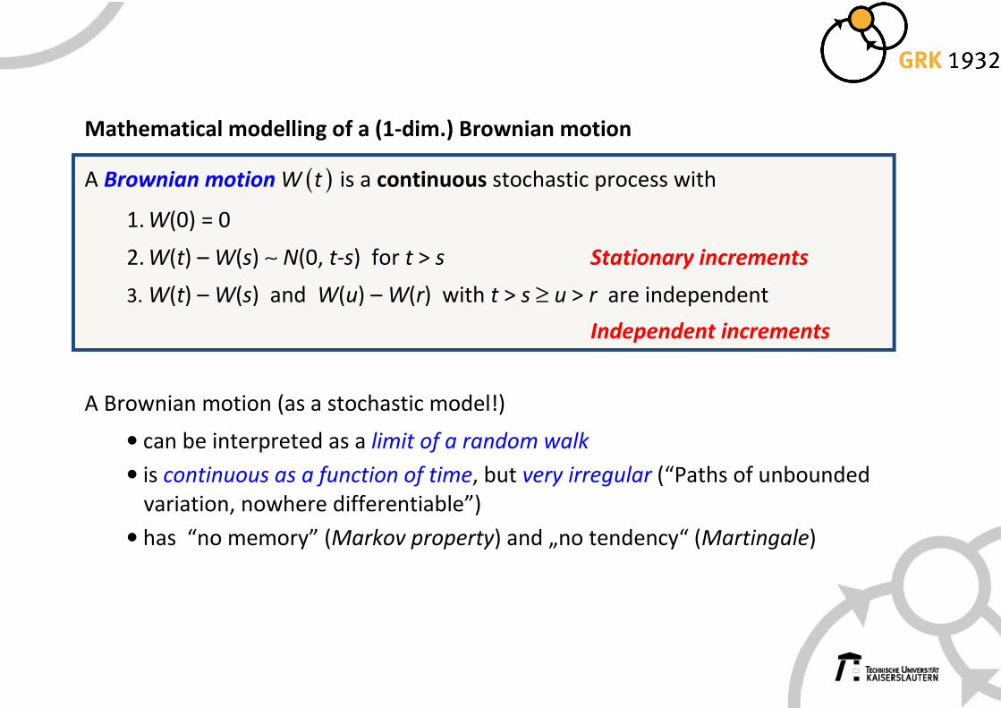
Mathematical modelling of a (1-dim.) Brownian motion

A Brownian motion ( )W t is a continuous stochastic process with

1. W(0) = 0

2. W(t) – W(s) ∼ N(0, t-s) for t > s Stationary increments

3. W(t) – W(s) and W(u) – W(r) with t > s ≥ u > r are independent

Independent increments

A Brownian motion (as a stochastic model!)

• can be interpreted as a limit of a random walk

• is continuous as a function of time, but very irregular (“Paths of unbounded

variation, nowhere differentiable”)

• has “no memory” (Markov property) and „no tendency“ (Martingale)

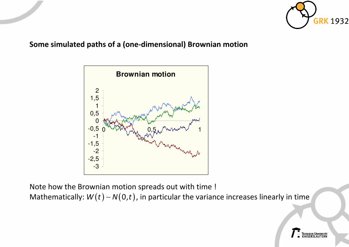
Some simulated paths of a (one-dimensional) Brownian motion

Note how the Brownian motion spreads out with time !

Mathematically: ( ) ( )0W t N ,t∼ , in particular the variance increases linearly in time

Brownian motion

-3

-2,5

-2

-1,5

-1

-0,5

0

0,5

1

1,5

2

0 0,5 1

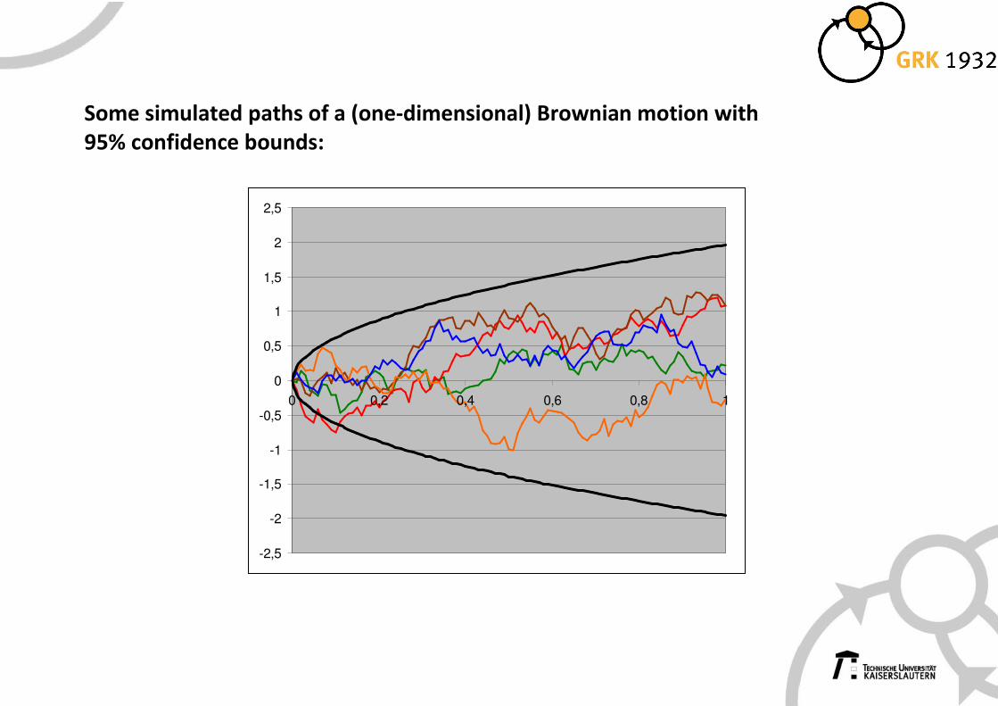
Some simulated paths of a (one-dimensional) Brownian motion with

95% confidence bounds:

-2,5

-2

-1,5

-1

-0,5

0

0,5

1

1,5

2

2,5

0 0,2 0,4 0,6 0,8 1

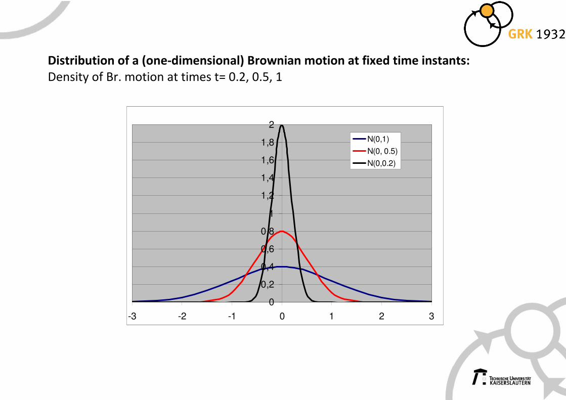
Distribution of a (one-dimensional) Brownian motion at fixed time instants:

Density of Br. motion at times t= 0.2, 0.5, 1

0

0,2

0,4

0,6

0,8

1

1,2

1,4

1,6

1,8

2

-3 -2 -1 0 1 2 3

N(0,1)

N(0, 0.5)

N(0,0.2)

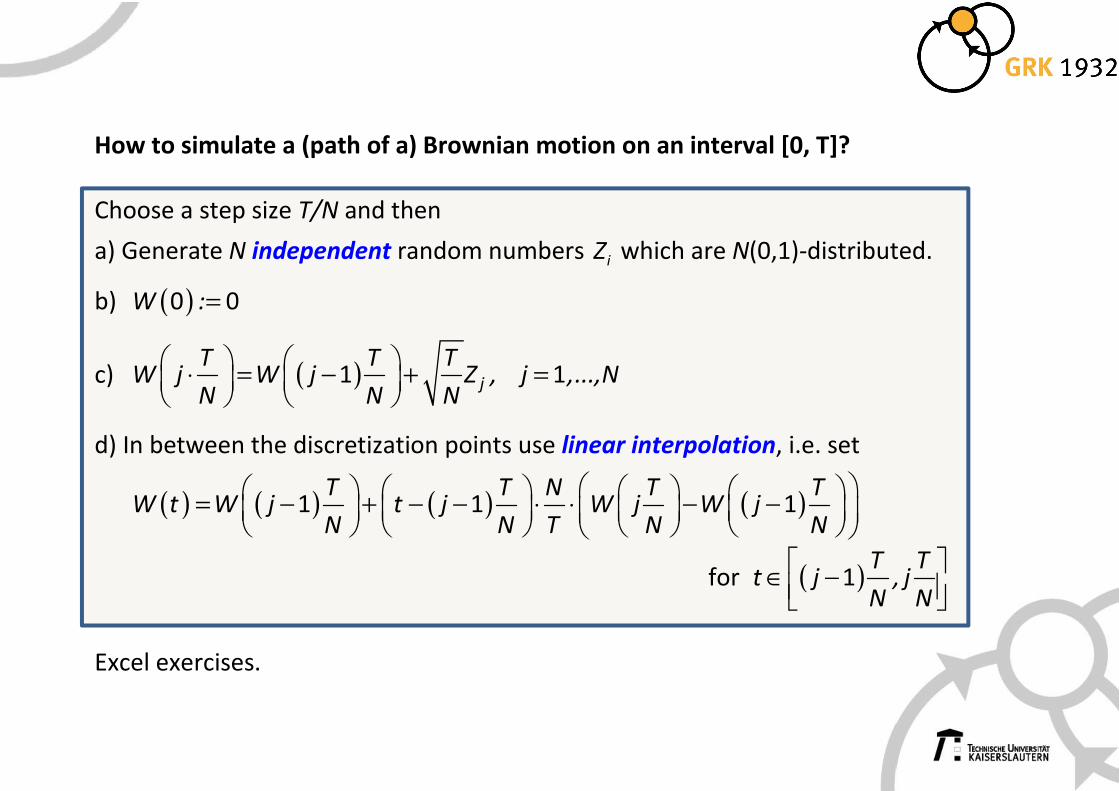
How to simulate a (path of a) Brownian motion on an interval [0, T]?

Choose a step size T/N and then

a) Generate N independent random numbers iZ which are N(0,1)-distributed.

b) ( )0 0W :=

c) ( )1 1j

T T TW j W j Z , j ,...,N

N N N

⋅ = − + =

d) In between the discretization points use linear interpolation, i.e. set

( ) ( ) ( ) ( )1 1 1T T N T T

W t W j t j W j W jN N T N N

= − + − − ⋅ ⋅ − −

for ( )1T T

t j , jN N

∈ −

Excel exercises.

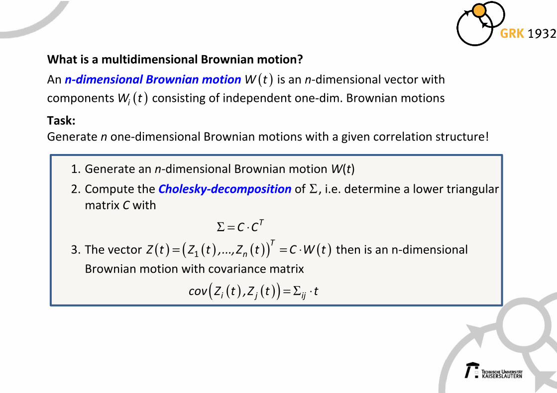
What is a multidimensional Brownian motion?

An n-dimensional Brownian motion ( )W t is an n-dimensional vector with

components ( )iW t consisting of independent one-dim. Brownian motions

Task:

Generate n one-dimensional Brownian motions with a given correlation structure!

1. Generate an n-dimensional Brownian motion W(t)

2. Compute the Cholesky-decomposition of Σ , i.e. determine a lower triangular

matrix C with

TC CΣ = ⋅

3. The vector ( ) ( ) ( )( ) ( )1

T

nZ t Z t ,...,Z t C W t= = ⋅ then is an n-dimensional

Brownian motion with covariance matrix

( ) ( )( )i j ijcov Z t ,Z t t= Σ ⋅

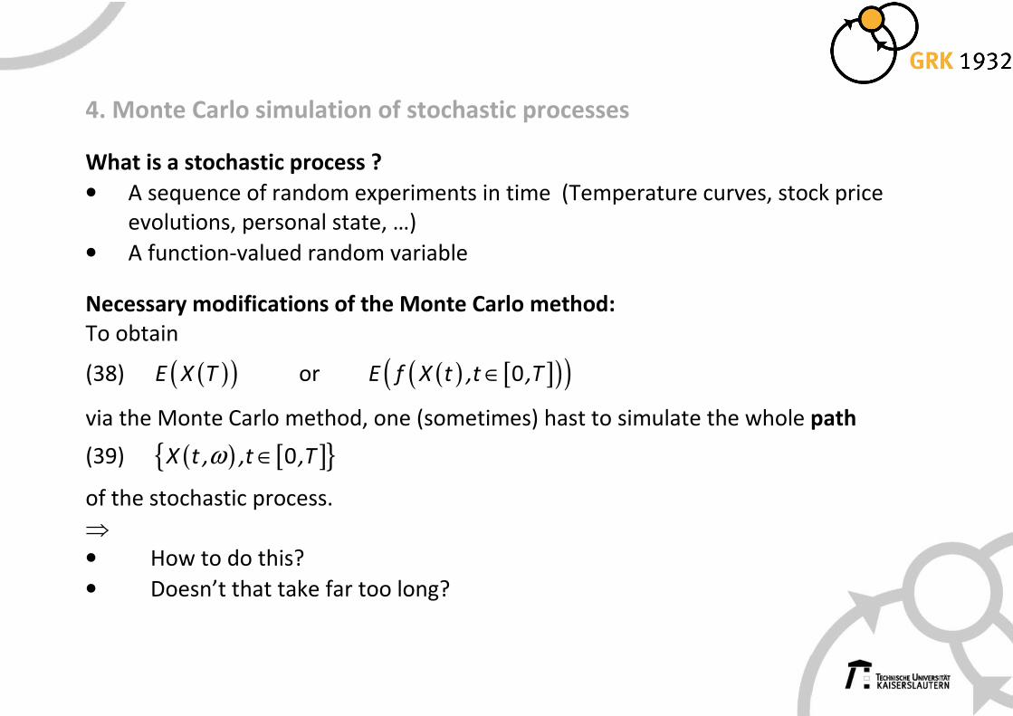
4. Monte Carlo simulation of stochastic processes

What is a stochastic process ?

• A sequence of random experiments in time (Temperature curves, stock price

evolutions, personal state, …)

• A function-valued random variable

Necessary modifications of the Monte Carlo method:

To obtain

(38) ( )( )E X T or ( ) [ ]( )( )0E f X t ,t ,T∈

via the Monte Carlo method, one (sometimes) hast to simulate the whole path

(39) ( ) [ ]{ }0X t , ,t ,Tω ∈

of the stochastic process.

⇒

• How to do this?

• Doesn’t that take far too long?

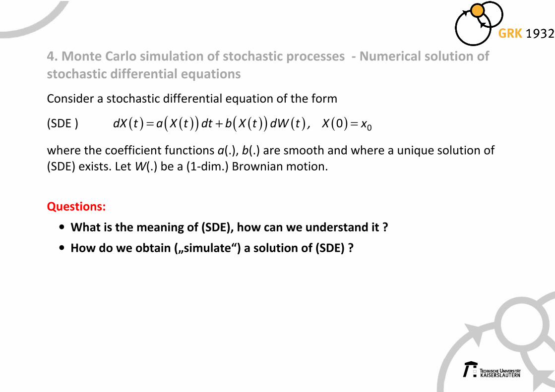
4. Monte Carlo simulation of stochastic processes - Numerical solution of

stochastic differential equations

Consider a stochastic differential equation of the form

(SDE ) ( ) ( )( ) ( )( ) ( ) ( ) 00dX t a X t dt b X t dW t , X x= + =

where the coefficient functions a(.), b(.) are smooth and where a unique solution of

(SDE) exists. Let W(.) be a (1-dim.) Brownian motion.

Questions:

• What is the meaning of (SDE), how can we understand it ?

• How do we obtain („simulate“) a solution of (SDE) ?

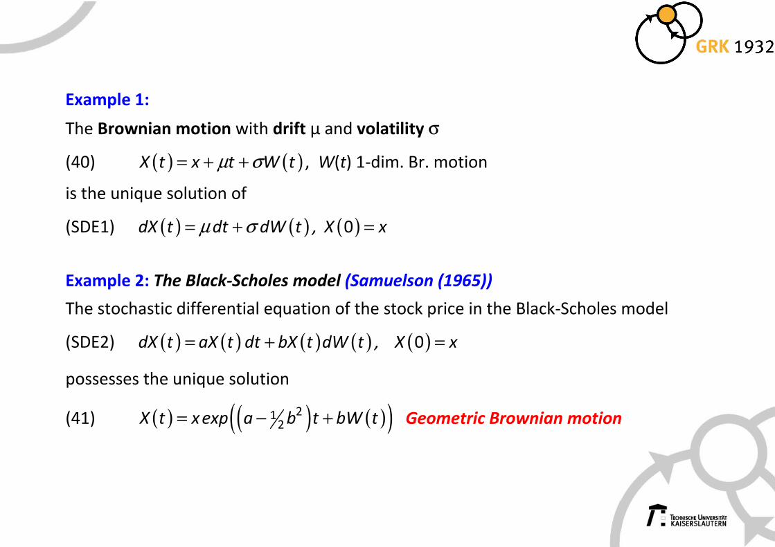
Example 1:

The Brownian motion with drift µ and volatility σ

(40) ( ) ( )X t x t W tµ σ= + + , W(t) 1-dim. Br. motion

is the unique solution of

(SDE1) ( ) ( ) ( )0dX t dt dW t , X xµ σ= + =

Example 2: The Black-Scholes model (Samuelson (1965))

The stochastic differential equation of the stock price in the Black-Scholes model

(SDE2) ( ) ( ) ( ) ( ) ( )0dX t aX t dt bX t dW t , X x= + =

possesses the unique solution

(41) ( ) ( ) ( )( )212X t x exp a b t bW t= − + Geometric Brownian motion

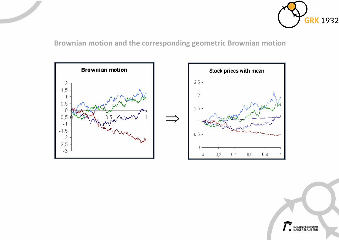
Brownian motion and the corresponding geometric Brownian motion

⇒

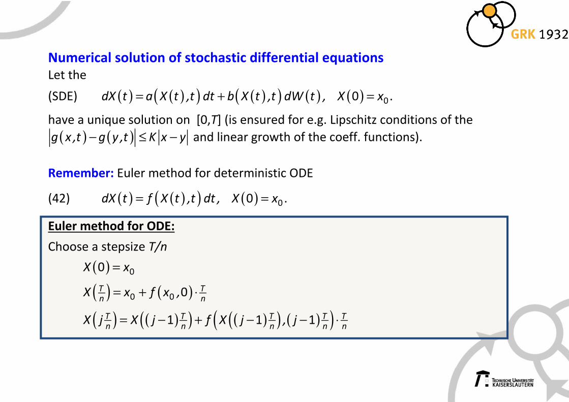
Numerical solution of stochastic differential equations

Let the

(SDE) ( ) ( )( ) ( )( ) ( ) ( ) 00dX t a X t ,t dt b X t ,t dW t , X x= + = .

have a unique solution on [0,T] (is ensured for e.g. Lipschitz conditions of the

( ) ( )g x ,t g y ,t K x y− ≤ − and linear growth of the coeff. functions).

Remember: Euler method for deterministic ODE

(42) ( ) ( )( ) ( ) 00dX t f X t ,t dt , X x= = .

Euler method for ODE:

Choose a stepsize T/n

( ) 00X x=

( ) ( )0 0 0T Tn n

X x f x ,= + ⋅

( ) ( )( ) ( )( ) ( )( )1 1 1T T T T Tn n n n n

X j X j f X j , j= − + − − ⋅

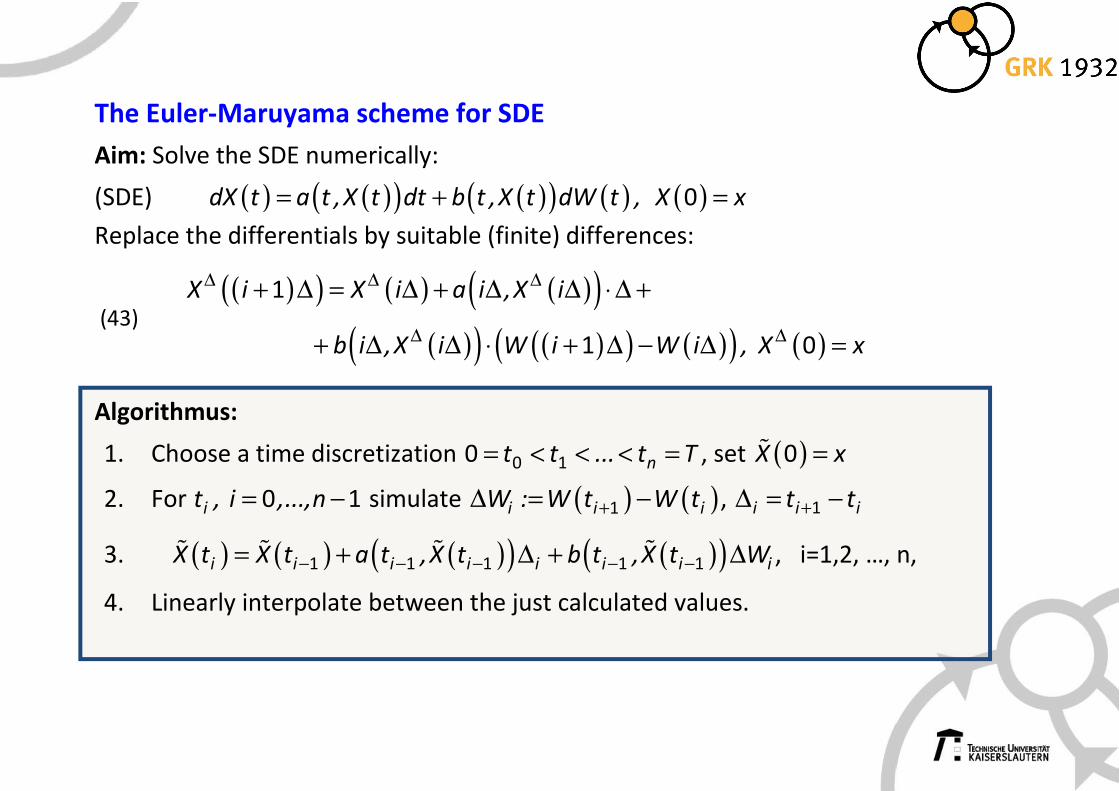
The Euler-Maruyama scheme for SDE

Aim: Solve the SDE numerically:

(SDE) ( ) ( )( ) ( )( ) ( ) ( )0dX t a t ,X t dt b t ,X t dW t , X x= + =

Replace the differentials by suitable (finite) differences:

(43)

( )( ) ( ) ( )( )( )( ) ( )( ) ( )( ) ( )

1

1 0

X i X i a i ,X i

b i ,X i W i W i , X x

∆ ∆ ∆

∆ ∆

+ ∆ = ∆ + ∆ ∆ ⋅ ∆ +

+ ∆ ∆ ⋅ + ∆ − ∆ =

Algorithmus:

1. Choose a time discretization 0 10 nt t ... t T= < < < = , set ( )0X x=ɶ

2. For 0 1it , i ,...,n= − simulate ( ) ( )1i i iW : W t W t+∆ = − , 1i i it t+∆ = −

3. ( ) ( ) ( )( ) ( )( )1 1 1 1 1i i i i i i i iX t X t a t ,X t b t ,X t W− − − − −= + ∆ + ∆ɶ ɶ ɶ ɶ , i=1,2, …, n,

4. Linearly interpolate between the just calculated values.

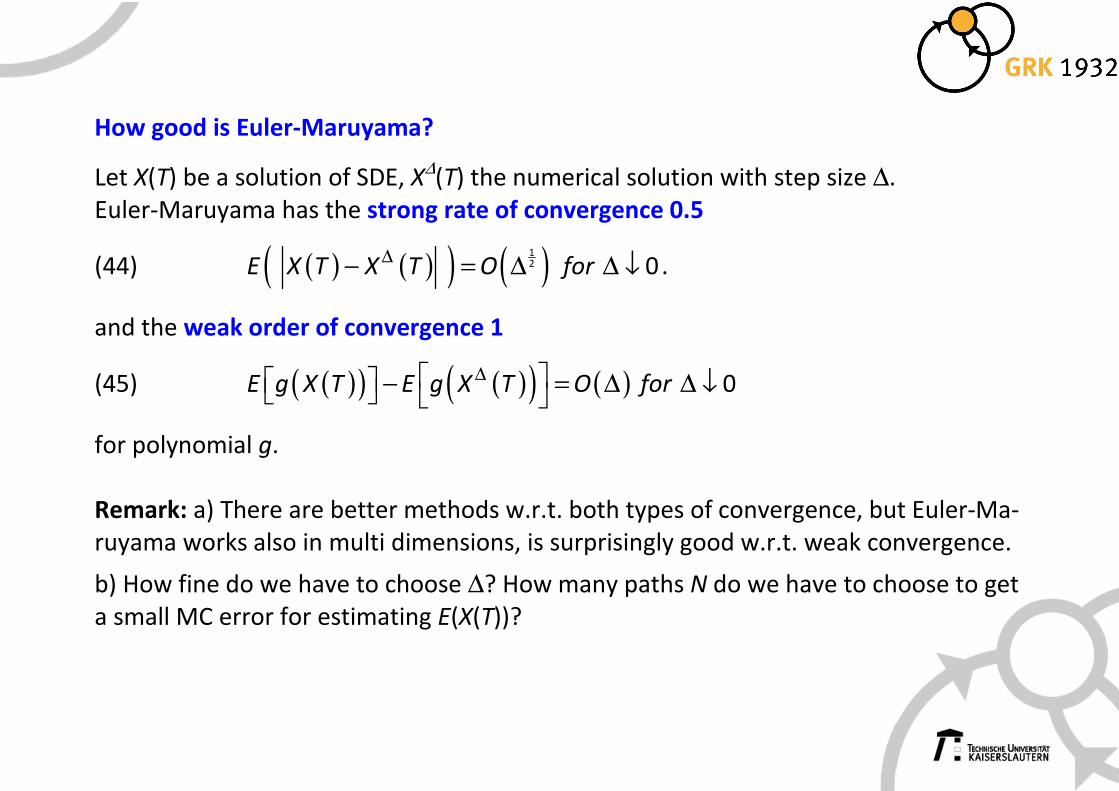
How good is Euler-Maruyama?

Let X(T) be a solution of SDE, X∆(T) the numerical solution with step size ∆.

Euler-Maruyama has the strong rate of convergence 0.5

(44) ( ) ( )( ) ( )12 0E X T X T O for

∆− = ∆ ∆ ↓ .

and the weak order of convergence 1

(45) ( )( ) ( )( ) ( ) 0E g X T E g X T O for∆ − = ∆ ∆ ↓

for polynomial g.

Remark: a) There are better methods w.r.t. both types of convergence, but Euler-Ma-

ruyama works also in multi dimensions, is surprisingly good w.r.t. weak convergence.

b) How fine do we have to choose ∆? How many paths N do we have to choose to get

a small MC error for estimating E(X(T))?

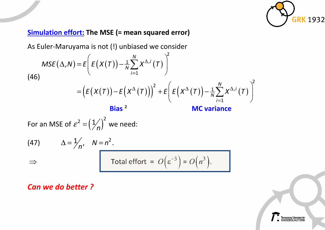
Simulation effort: The MSE (= mean squared error)

As Euler-Maruyama is not (!) unbiased we consider

(46)

( ) ( )( ) ( )

( )( ) ( )( )( ) ( )( ) ( )

2

1

1

22

1

1

N,i

Ni

N,i

Ni

MSE ,N E E X T X T

E X T E X T E E X T X T

∆

=

∆ ∆ ∆

=

∆ = −

= − + −

∑

∑

Bias ² MC variance

For an MSE of ( )22 1

nε = we need:

(47) 1n

∆ = , 2N n= .

⇒ Total effort = ( )3O

−ε = ( )3O n .

Can we do better ?

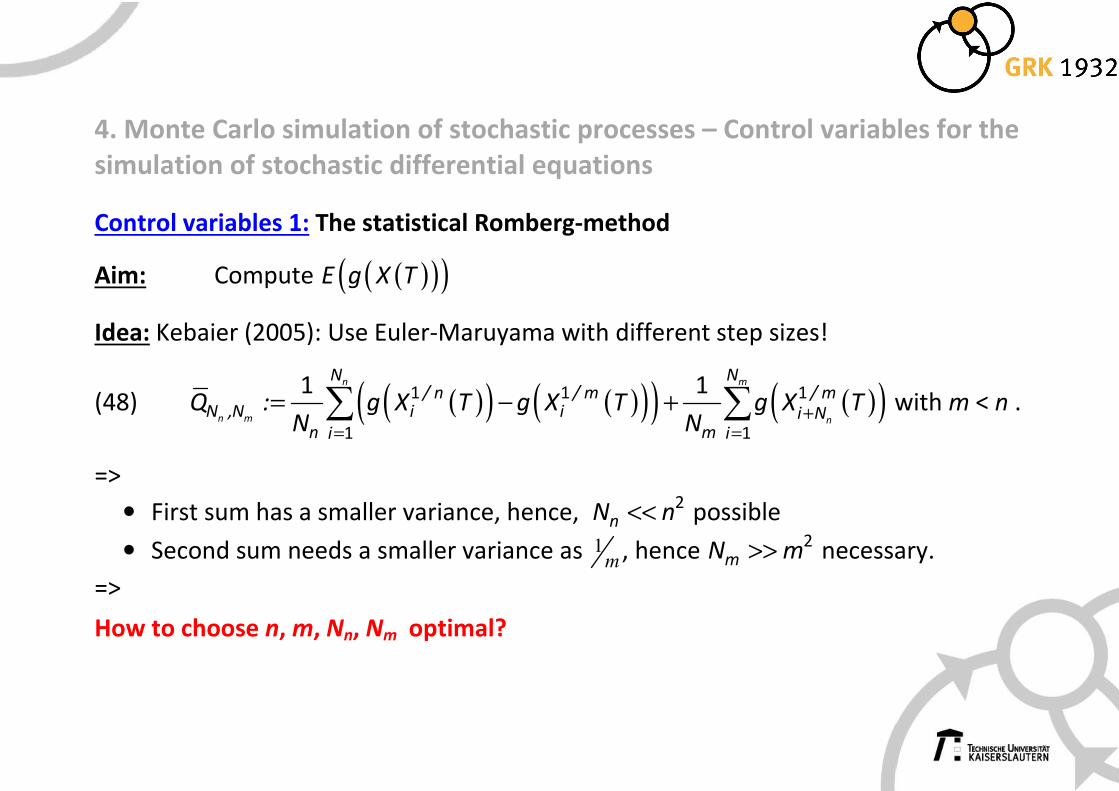
4. Monte Carlo simulation of stochastic processes – Control variables for the

simulation of stochastic differential equations

Control variables 1: The statistical Romberg-method

Aim: Compute ( )( )( )E g X T

Idea: Kebaier (2005): Use Euler-Maruyama with different step sizes!

(48) ( )( ) ( )( )( ) ( )( )1 1 1

1 1

1 1n m

n m n

N N/ n / m / m

N ,N i i i Nn mi i

Q : g X T g X T g X TN N

+= =

= − +∑ ∑ with m < n .

=>

• First sum has a smaller variance, hence, 2nN n<< possible

• Second sum needs a smaller variance as 1m , hence 2

mN m>> necessary.

=>

How to choose n, m, Nn, Nm optimal?

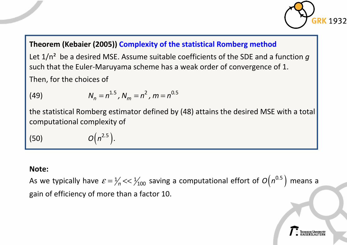
Theorem (Kebaier (2005)) Complexity of the statistical Romberg method

Let 1/n² be a desired MSE. Assume suitable coefficients of the SDE and a function g

such that the Euler-Maruyama scheme has a weak order of convergence of 1.

Then, for the choices of

(49) 1 5 2 0 5. .n mN n , N n , m n= = =

the statistical Romberg estimator defined by (48) attains the desired MSE with a total

computational complexity of

(50) ( )2 5.O n .

Note:

As we typically have 1 1100nε = << saving a computational effort of ( )0 5.

O n means a

gain of efficiency of more than a factor 10.

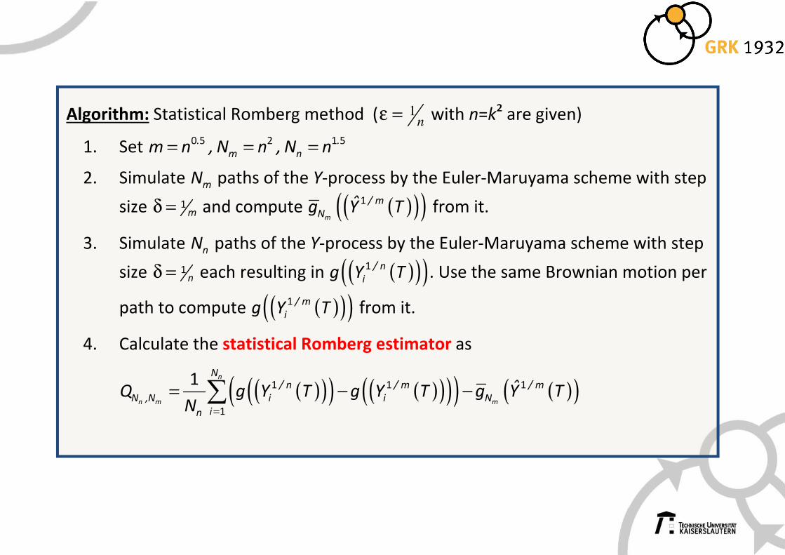
Algorithm: Statistical Romberg method ( 1nε = with n=k² are given)

1. Set 0 5 2 1 5. .

m nm n , N n , N n= = =

2. Simulate mN paths of the Y-process by the Euler-Maruyama scheme with step

size 1mδ = and compute ( )( )( )1

m

/ m

Nˆg Y T from it.

3. Simulate nN paths of the Y-process by the Euler-Maruyama scheme with step

size 1nδ = each resulting in ( )( )( )1 / n

ig Y T . Use the same Brownian motion per

path to compute ( )( )( )1 / m

ig Y T from it.

4. Calculate the statistical Romberg estimator as

( )( )( ) ( )( )( )( ) ( )( )1 1 1

1

1 n

n m m

N/ n / m / m

N ,N i i N

in

ˆQ g Y T g Y T g Y TN =

= − −∑

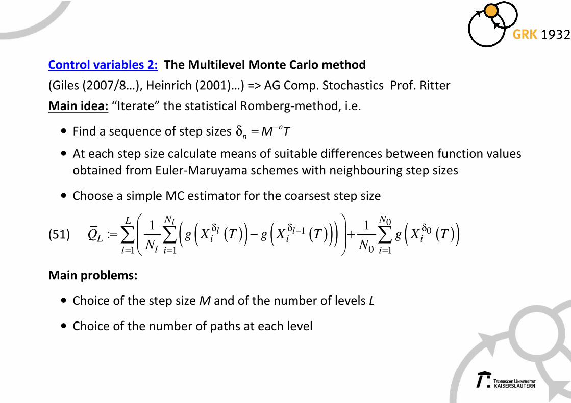
Control variables 2: The Multilevel Monte Carlo method

(Giles (2007/8…), Heinrich (2001)…) => AG Comp. Stochastics Prof. Ritter

Main idea: “Iterate” the statistical Romberg-method, i.e.

• Find a sequence of step sizes n

n M T−δ =

• At each step size calculate means of suitable differences between function values

obtained from Euler-Maruyama schemes with neighbouring step sizes

• Choose a simple MC estimator for the coarsest step size

(51)

Main problems:

• Choice of the step size M and of the number of levels L

• Choice of the number of paths at each level

( )( ) ( )( )( ) ( )( )0

1 0

01 1 1

1 1:

ll l

N NL

L i i ill i i

Q g X T g X T g X TN N

−δ δ δ

= = =

= − +

∑ ∑ ∑

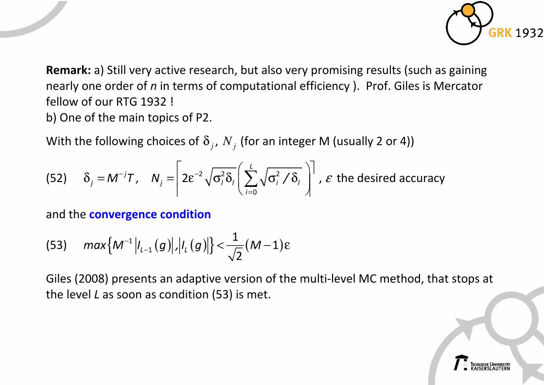
Remark: a) Still very active research, but also very promising results (such as gaining

nearly one order of n in terms of computational efficiency ). Prof. Giles is Mercator

fellow of our RTG 1932 !

b) One of the main topics of P2.

With the following choices of jδ , jN (for an integer M (usually 2 or 4))

(52) j

j M T−δ = , 2 2 2

0

2L

j l l i l

i

N /−

=

= ε σ δ σ δ

∑ , ε the desired accuracy

and the convergence condition

(53) ( ) ( ){ } ( )1

1

11

2L Lmax M I g , I g M

−− < − ε

Giles (2008) presents an adaptive version of the multi-level MC method, that stops at

the level L as soon as condition (53) is met.

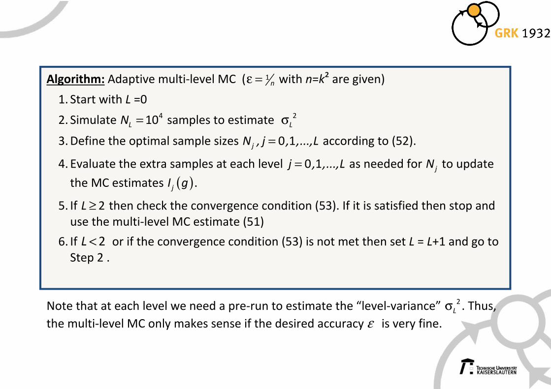
Algorithm: Adaptive multi-level MC ( 1nε = with n=k² are given)

1. Start with L =0

2. Simulate 410LN = samples to estimate 2

Lσ

3. Define the optimal sample sizes 0 1jN , j , ,...,L= according to (52).

4. Evaluate the extra samples at each level 0 1j , ,...,L= as needed for jN to update

the MC estimates ( )jI g .

5. If 2L ≥ then check the convergence condition (53). If it is satisfied then stop and

use the multi-level MC estimate (51)

6. If 2L < or if the convergence condition (53) is not met then set L = L+1 and go to

Step 2 .

Note that at each level we need a pre-run to estimate the “level-variance” 2

Lσ . Thus,

the multi-level MC only makes sense if the desired accuracy ε is very fine.

Literature for Talk 2:

Giles M. (2007) Improved multilevel Monte Carlo convergence using the Milstein

scheme. Monte Carlo and Quasi-Monte Carlo Methods 2006, Springer, 343-358.

Giles M. (2008) Multi-level Monte Carlo path simulation. Operations Research, 56(3),

607-617.

Glasserman P. (2004) Monte Carlo methods in financial engineering. Springer.

Kanj R., Joshi R., Nassif S. (2006) Mixture importance sampling and its application to

the analysis of SRAM designs in the presence of rare failure events, DAC, 69-72.

Kebaier A. (2005) Statistical Romberg extrapolation: a new variance reduction method

and applications to option pricing. Annals of Applied Probability, 15(4), 2681-2705.

Korn E., Korn R., Kroisandt G. (2010) Monte Carlo Methods and Models in Finance and

Insurance. Chapman & Hall, Chapter 4.

5. Sensitivity analysis of Monte Carlo results

A practical question:

How strong do results of a Monte Carlo computation depend on the intial input

parameters?

(Naive) Idea:

Simply repeat the computations with different input parameters and look at the

effects.

Assume:

• The stochastic process P(t) depends on the input parameter y

• We want to calculate X(0) = X(0;y) = E(f(P(T)))

• How to calculate

(1) ( )0X ;y

y

∂

∂

5. MC-sensitivities with finite differences

Idea:

Approximate ( )0X ;yy

∂

∂ by finite differences:

(2) ( ) ( )0 0X ;y h X ;y

h

+ −. “forward differences”

(3) ( ) ( )0 0

2

X ;y h X ;y h

h

+ − −. “central differences”

How to do this:

• Use the same paths of Brownian motion to compute ( ) ( )0 0X ;y h , X ;y± by

Monte Carlo methods (or by some other method) “Paths recycling”

• Compute one of the above finite differences for a suitable h

Note:

• Optimal choice: central differences with h = 1 4/ε (where ε =machine accuracy)

• Finite differences are easy to implement but often not the method of choice

5. MC-sensitivities with pathwise differentiation

Idea:

Approximate ( ) ( ) ( )( )( )00

;yX ;y E g P T

y y

∂ ∂=

∂ ∂ by exchanging differentiation and

calculating expectation:

(4) ( ) ( ) ( )( ) ( )00

;yX ;y E g' P T P T

y y

∂ ∂ = ∂ ∂

How to do this:

• Check if it is allowed to perform the above exchangement (i.e. check assump. of

montone convergence, dominated convergence or …)

• Compute the relevant derivatives and then calculate the expectation by Monte

Carlo methods (or by some other method)

Note:

• When applicable then pathwise differentiation often is the method of choice

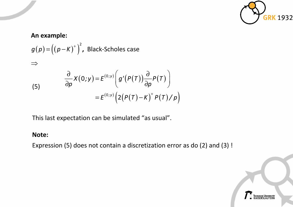
An example:

( ) ( )( )2

g p p K+

= − , Black-Scholes case

⇒

(5) ( ) ( ) ( )( ) ( )

( ) ( )( ) ( )( )

0

0

0

2

;y

;y

X ;y E g' P T P Tp p

E P T K P T / p+

∂ ∂ = ∂ ∂

= −

This last expectation can be simulated “as usual”.

Note:

Expression (5) does not contain a discretization error as do (2) and (3) !

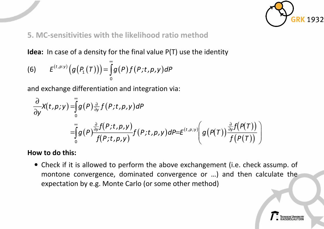
5. MC-sensitivities with the likelihood ratio method

Idea: In case of a density for the final value P(T) use the identity

(6) ( ) ( )( )( ) ( ) ( )1

0

t ,p:yE g P T g P f P ;t ,p,y dP

∞

= ∫

and exchange differentiation and integration via:

( ) ( ) ( )

( )( )

( )( ) ( ) ( )( )

( )( )( )( )

0

0

y

y yt ,p ;y

X t ,p;y g P f P ;t ,p,y dPy

f P ;t ,p,y f P Tg P f P ;t ,p,y dP E g P T

f P ;t ,p,y f P T

∞∂∂

∞ ∂ ∂∂ ∂

∂=

∂

= =

∫

∫

How to do this:

• Check if it is allowed to perform the above exchangement (i.e. check assump. of

montone convergence, dominated convergence or …) and then calculate the

expectation by e.g. Monte Carlo (or some other method)

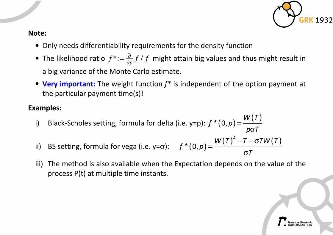
Note:

• Only needs differentiability requirements for the density function

• The likelihood ratio *: /y

f f f∂∂

= might attain big values and thus might result in

a big variance of the Monte Carlo estimate.

• Very important: The weight function f* is independent of the option payment at

the particular payment time(s)!

Examples:

i) Black-Scholes setting, formula for delta (i.e. y=p): ( )( )

0W T

f * ,pp T

=σ

ii) BS setting, formula for vega (i.e. y=σ): ( )( ) ( )2

0W T T TW T

f * ,pT

− − σ=

σ

iii) The method is also available when the Expectation depends on the value of the

process P(t) at multiple time instants.

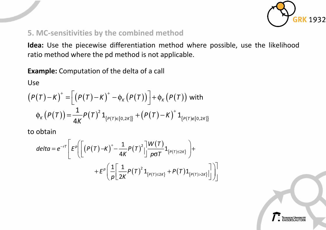
5. MC-sensitivities by the combined method

Idea: Use the piecewise differentiation method where possible, use the likelihood

ratio method where the pd method is not applicable.

Example: Computation of the delta of a call

Use

( )( ) ( )( ) ( )( ) ( )( )K KP T K P T K P T P T+ + − = − − φ + φ

with

( )( ) ( ) ( ) [ ]{ } ( )( ) ( ) [ ]{ }2

0 2 0 2

11 1

4K P T , K P T , K

P T P T P T KK

+

∈ ∉φ = + −

to obtain

( )( ) ( )

( )( ){ }

( ) ( ){ } ( ) ( ){ }

2

2

2

2 2

11

4

1 11 1

2

rT p

P T K

p

P T K P T K

W Tdelta e E P T K P T

K p T

E P T P Tp K

+−≤

≤ >

= − − + σ

+ +

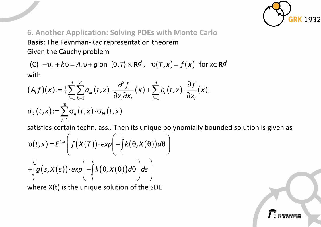
6. Another Application: Solving PDEs with Monte Carlo

Basis: The Feynman-Kac representation theorem

Given the Cauchy problem

(C) t tk A g−υ + υ = υ + on [0,T) × Rd , ( ) ( )T ,x f xυ = for x∈Rd

with

( )( ) ( ) ( ) ( ) ( ) :=

2

12

1 1 1

d d d

t ik i

i k ii k i

ffA f x a t ,x x b t ,x x

x x x= = =

∂∂⋅ + ⋅∂ ∂ ∂

∑∑ ∑ ,

( ) ( ) ( ) := 1

m

ik ij kj

j

a t ,x t ,x t ,x=

σ ⋅σ∑

satisfies certain techn. ass.. Then its unique polynomially bounded solution is given as

( ) ( )( ) ( )( )T

t ,x

t

t ,x E f X T exp k ,X d

υ = ⋅ − θ θ θ ∫

( )( ) ( )( )T s

t t

g s,X s exp k ,X d ds

+ ⋅ − θ θ θ

∫ ∫

where X(t) is the unique solution of the SDE

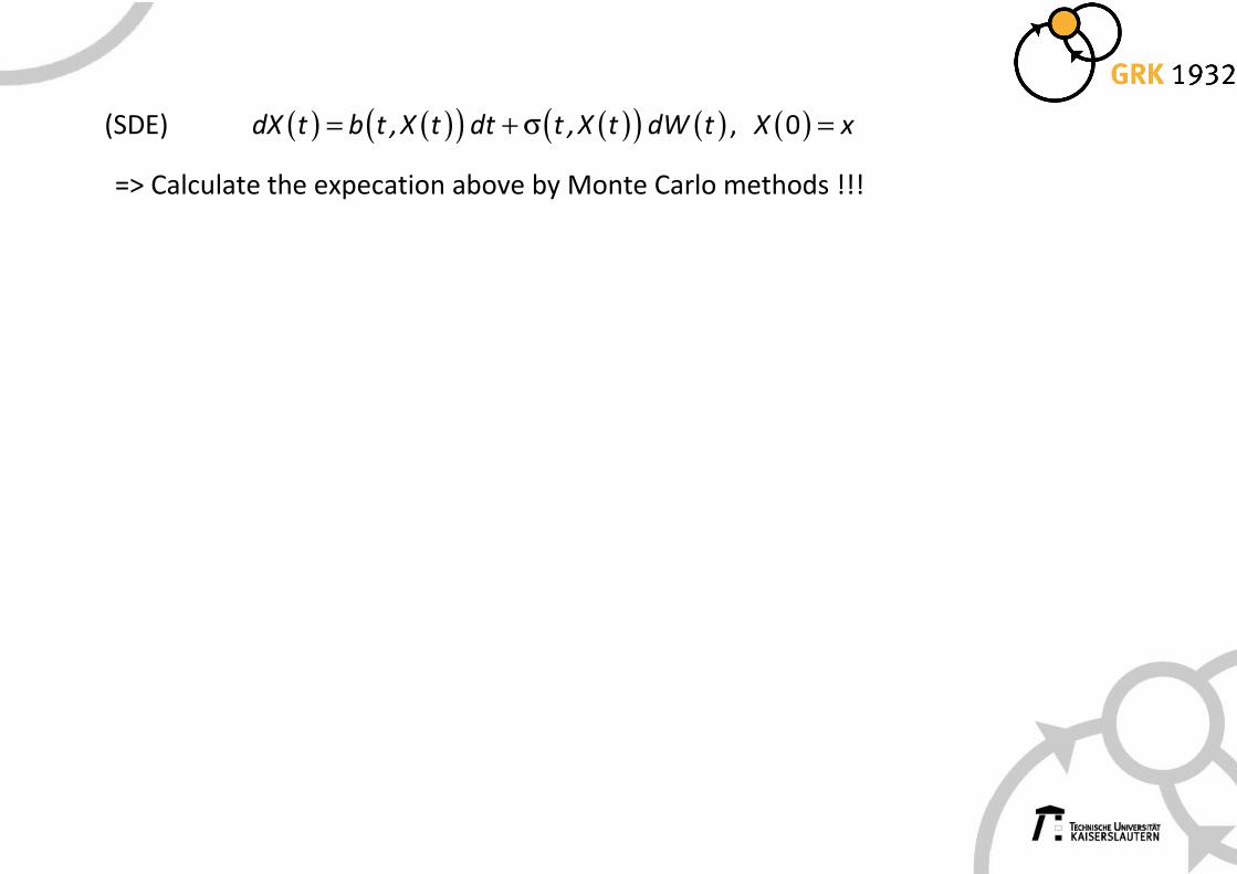
(SDE) ( ) ( )( ) ( )( ) ( )dX t b t ,X t dt t ,X t dW t= + σ , ( )0X x=

=> Calculate the expecation above by Monte Carlo methods !!!

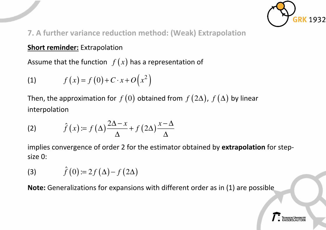
7. A further variance reduction method: (Weak) Extrapolation

Short reminder: Extrapolation

Assume that the function ( )f x has a representation of

(1) ( ) ( ) ( )20f x f C x O x= + ⋅ +

Then, the approximation for ( )0f obtained from ( )2f ∆ , ( )f ∆ by linear

interpolation

(2) ( ) ( ) ( )2ˆ : 2x x

f x f f∆ − − ∆

= ∆ + ∆∆ ∆

implies convergence of order 2 for the estimator obtained by extrapolation for step-

size 0:

(3) ( ) ( ) ( )ˆ 0 : 2 2f f f= ∆ − ∆

Note: Generalizations for expansions with different order as in (1) are possible

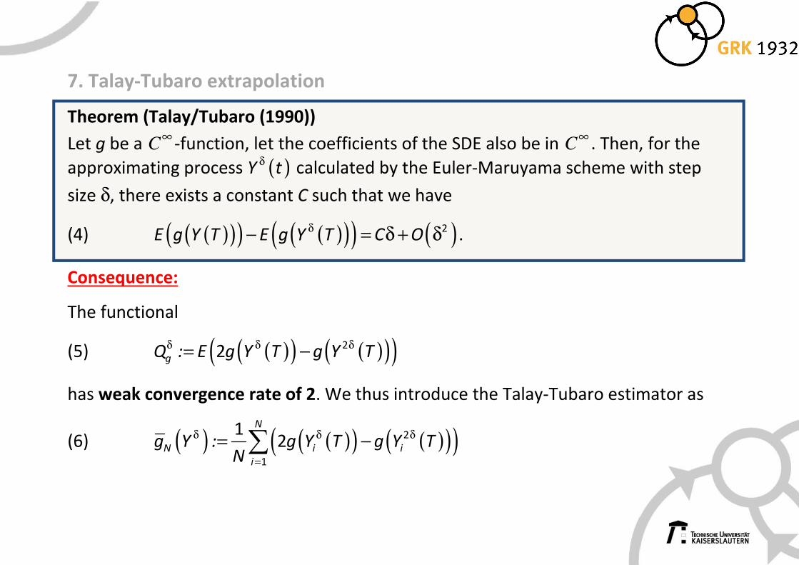
7. Talay-Tubaro extrapolation

Theorem (Talay/Tubaro (1990))

Let g be a C∞ -function, let the coefficients of the SDE also be in C∞ . Then, for the

approximating process ( )Y tδ calculated by the Euler-Maruyama scheme with step

size δ, there exists a constant C such that we have

(4) ( )( )( ) ( )( )( ) ( )2E g Y T E g Y T C O

δ− = δ + δ .

Consequence:

The functional

(5) ( )( ) ( )( )( )22gQ : E g Y T g Y Tδ δ δ= −

has weak convergence rate of 2. We thus introduce the Talay-Tubaro estimator as

(6) ( ) ( )( ) ( )( )( )2

1

12

N

N i i

i

g Y : g Y T g Y TN

δ δ δ

=

= −∑

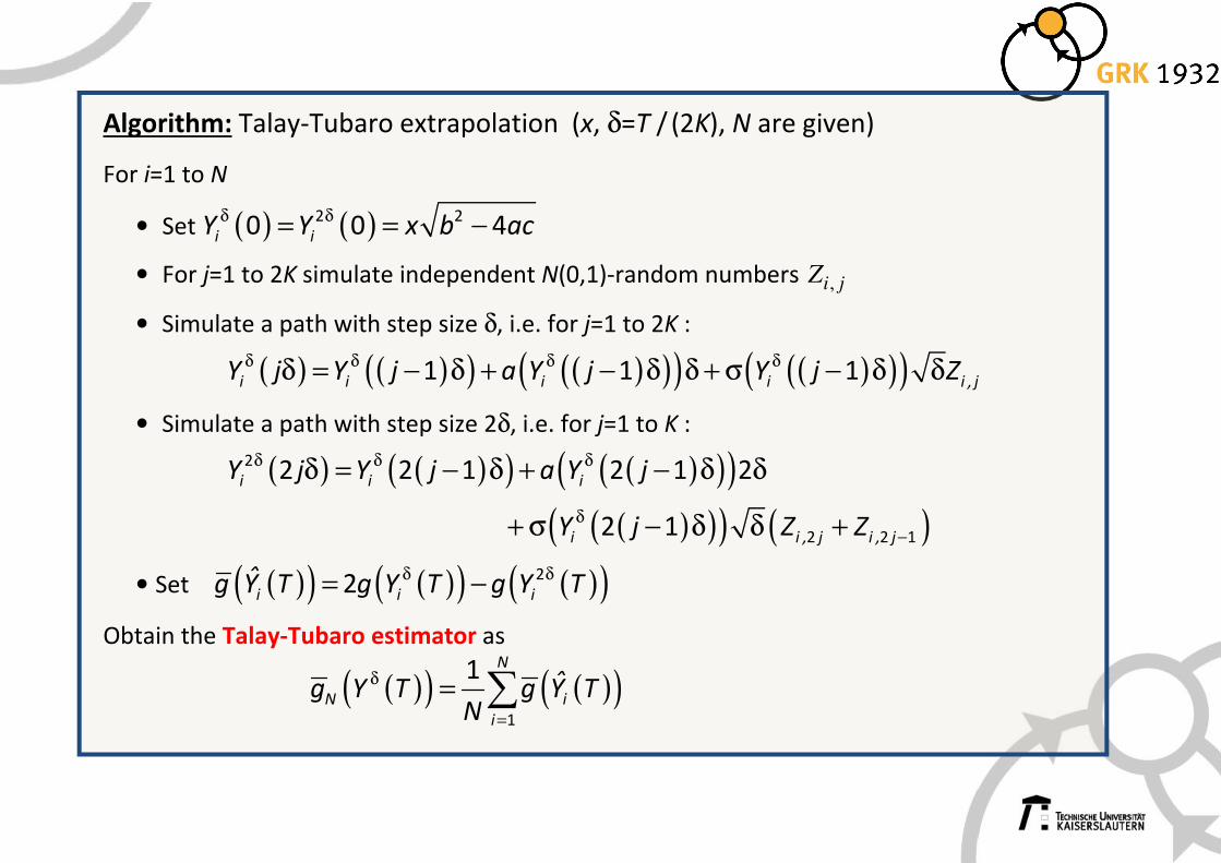
Algorithm: Talay-Tubaro extrapolation (x, δ=T / (2K), N are given)

For i=1 to N

• Set ( ) ( )2 20 0 4i iY Y x b acδ δ= = −

• For j=1 to 2K simulate independent N(0,1)-random numbers ,i jZ

• Simulate a path with step size δ, i.e. for j=1 to 2K :

( ) ( )( ) ( )( )( ) ( )( )( )1 1 1i i i i i , jY j Y j a Y j Y j Zδ δ δ δδ = − δ + − δ δ + σ − δ δ

• Simulate a path with step size 2δ, i.e. for j=1 to K :

( ) ( )( ) ( )( )( )

( )( )( ) ( )

2

2 2 1

2 2 1 2 1 2

2 1

i i i

i i , j i , j

Y j Y j a Y j

Y j Z Z

δ δ δ

δ−

δ = − δ + − δ δ

+ σ − δ δ +

• Set ( )( ) ( )( ) ( )( )22i i iˆg Y T g Y T g Y T

δ δ= −

Obtain the Talay-Tubaro estimator as

( )( ) ( )( )1

1 N

N i

i

ˆg Y T g Y TN

δ

=

= ∑

8. Further aspects

• Simulating more general stochastic processes (jump processes, Lévy processes

…)

• Monte Carlo simulation in space and space/time (=> P1, P4)

• An application: Solving partial partial differential equations with Monte Carlo

methods

• Markov Chain Monte Carlo: Simulating distributions you cannot simulate

• Monte Carlo and parallelization (=> P2)

• Quasi-Monte Carlo methods: Deterministic methods in a Monte Carlo setting

⇒ Given your wishes, these topics can all be dealt with during the next months

Literature for Talk 3:

Korn E., Korn R., Kroisandt G. (2010) Monte Carlo Methods and Models in Finance and

Insurance. Chapman & Hall.