monte carlo integration with acceptance-rejection · 2017-06-28 · monte carlo integration with...

Monte Carlo Integration WithAcceptance-Rejection

Zhiqiang TAN

This article considers Monte Carlo integration under rejection sampling orMetropolis-Hastings sampling Each algorithm involves accepting or rejecting observa-tions from proposal distributions other than a target distribution While taking a likeli-hood approach we basically treat the sampling scheme as a random design and definea stratified estimator of the baseline measure We establish that the likelihood estimatorhas no greater asymptotic variance than the crude Monte Carlo estimator under rejectionsampling or independence Metropolis-Hastings sampling We employ a subsamplingtechnique to reduce the computational cost and illustrate with three examples the com-putational effectiveness of the likelihood method under general Metropolis-Hastingssampling

Key Words Importance sampling Metropolis-Hastings sampling Rao-BlackwellizationRejection sampling Stratification Variance reduction

1 INTRODUCTION

In many problems of statistics it is of interest to compute expectations with respect to aprobability distribution For certain situations it is also necessary to estimate its normalizingconstant Specifically let q(x) be a nonnegative function on a state space X and considerthe probability distribution whose density is

p(x) =q(x)Z

with respect to a baseline measure micro0 where Z is the normalizing constantintq(x) dmicro0

Monte Carlo is a useful method for solving the aforementioned problems and typically hastwo parts simulation and estimation in its implementation

First a sequence of observations x1 xn are simulated from the distribution p(middot)Then the expectation Ep(ϕ) of a function ϕ(x) with respect to p(middot) can be estimated by the

Zhiqiang Tan is Assistant Professor Department of Biostatistics Bloomberg School of Public Health JohnsHopkins University 615 North Wolfe Street Baltimore MD 21205 (E-mail ztanjhsphedu)

ccopy 2006 American Statistical Association Institute of Mathematical Statisticsand Interface Foundation of North America

Journal of Computational and Graphical Statistics Volume 15 Number 3 Pages 735ndash752DOI 101198106186006X142681

735

736 Z TAN

sample average or the crude Monte Carlo (CMC) estimator

1n

nsumi=1

ϕ(xi) (11)

By letting ϕ(x) = q1(x)q(x) the normalizing constant Z can be estimated by(1n

nsumi=1

q1(xi)q(xi)

)minus1

(12)

where q1(x) is a probability density on X This estimator is called reciprocal importancesampling (RIS) see DiCiccio Kass Raftery and Wasserman (1997) and Gelfand and Dey(1994)

This article considers rejection sampling or Metropolis-Hastings sampling for the sim-ulation part Rejection sampling requires a probability density ρ(x) and a constant C suchthat q(x) le Cρ(x) on X which implies Z le C (von Neumann 1951) At each time t ge 1

bull Sample yt from ρ(middot)bull accept yt with probability q(yt)[Cρ(yt)] and move to the next trial otherwise

The second step can be implemented by generating ut from uniform (0 1) and acceptingyt if ut le q(yt)[Cρ(yt)] Then the accepted yt are independent and identically distributed(iid) as p(middot) To compare Metropolis-Hastings sampling requires a family of probabilitydensities ρ(middotx) x isin X (Metropolis et al 1953 Hastings 1970) At each time t ge 1

bull Sample yt from ρ(middotxtminus1)

bull accept xt = yt with probability 1 and β(ytxtminus1) and let xt = xtminus1 otherwise where

β(yx) =q(y)ρ(x y)q(x)ρ(yx)

The second step can also be implemented by generatingut from uniform (0 1) and acceptingxt = yt if ut le 1 and β(ytxtminus1) Under suitable regularity conditions the Markov chain(x1 x2 ) converges to the target distribution p(middot) In the so-called independence case(IMH) the proposal density ρ(middotx) equiv ρ(middot) is independent of x Then the chain is uniformlyergodic if q(x)ρ(x) is bounded from above on X and is not even geometrically ergodicotherwise (Mengersen and Tweedie 1996) The condition that q(x) le Cρ(x) on X isassumed henceforth

Neither rejection sampling nor Metropolis-Hastings sampling requires the value of thenormalizing constant Z However each algorithm involves accepting or rejecting obser-vations from proposal distributions Acceptance or rejection depends on uniform randomvariables By integrating out these uniform random variables Casella and Robert (1996)proposed a Rao-Blackwellized estimator that has no greater variance than the crude MonteCarlo estimator but they mostly disregarded the issue of computational time increased byRao-Blackwellization

Recently Kong et al (2003) formulated Monte Carlo integration as a statistical modelusing simulated observations as data The baseline measure is treated as the parameter and

MONTE CARLO INTEGRATION WITH ACCEPTANCE-REJECTION 737

estimated as a discrete measure by maximum likelihood Consequently integrals of interestare estimated as finite sums by substituting the estimated measure We take the likelihoodapproach and develop a method for estimating simultaneously the normalizing constantZ and the expectation Ep(ϕ) under rejection sampling (Section 2) or Metropolis-Hastingssampling (Section 3) This work can be considered as a concrete case of Tanrsquos (2003)methodology but its significance is worth singling out

Under rejection sampling or independence Metropolis-Hastings sampling computationof the estimated measure requires negligible effort We establish theoretical results that thelikelihood estimator of Ep(ϕ) has no greater asymptotic variance than the crude MonteCarlo estimator under each scheme These two facts together imply that the likelihoodmethod is always computationally more effective than crude Monte Carlo under rejectionsampling or independence Metropolis-Hastings sampling

Under general Metropolis-Hastings sampling computation of the estimated measureinvolves intensive evaluations of proposal densities Therefore we employ a subsamplingtechnique to reduce this computational cost We provide empirical evidence for the com-putational effectiveness of the likelihood method with three examples We also introduceapproximate variance estimators for the point estimators These estimators agree with theempirical variances from repeated simulations in all the examples

The proofs of all lemmas and theorems are collected in the Appendix Computations inSections 23 and 33 are programmed in MATLAB on Pentium 4 machines with CPU speedof 200 GHz

2 REJECTION SAMPLING

For clarity let us consider two cases separately In one case the number of trials is fixedwhile that of acceptances is random In the other case the number of acceptances is fixedwhile that of trials is random For illustration an example is provided

21 FIXED NUMBER OF TRIALS

Suppose that rejection sampling is run for a fixed number say n of trials In the processy1 yn are generated from ρ(middot) u1 un are from uniform (0 1) and acceptance oc-curs at t1 tL Then the number of acceptancesL has the binomial distribution (nZC)The expectation Ep(ϕ) can be estimated by

1L

Lsumi=1

ϕ(yti) (21)

This estimator is defined to be 0 if L = 0 which has positive probability for any finite n

Lemma 1 Assume that varρ(ϕ) lt infin where varρ denotes the variance under thedistribution ρ(middot) The estimator (21) has asymptotic variancenminus1(ZC)varp(ϕ) asn tendsto infinity where varp is the variance under the distribution p(middot)

In the likelihood approach we ignore the baseline measure (micro0) being Lebesgue orcounting and treat the ignored measure (micro) as the parameter in a model The parameter

738 Z TAN

space consists of nonnegative measures on X such thatintρ(x) dmicro is finite and positive The

model states that the data are generated as follows For each t ge 1

bull yt has the distribution ρ(middot) dmicro int ρ(y) dmicro

bull ut has the distribution uniform (0 1)

bull accept yt if ut le q(yt)[Cρ(yt)] and reject otherwise

It is easy to show that the accepted yt are independent and identically distributed asq(middot) dmicro int q(y) dmicro The likelihood of the process at micro is proportional to

nprodi=1

[ρ(yi)micro(yi)

intρ(y) dmicro

]

Any measure that does not place mass at each of the points y1 yn has zero likelihoodBy Jensenrsquos inequality the maximizing measure is given by

micro(y) prop Γ(y)ρ(y)

where Γ is the empirical distribution placing mass nminus1 at each of the points y1 ynConsequently the expectation Ep(ϕ) is estimated by

intϕ(y)q(y) dmicro

intq(y) dmicro or

nsumi=1

ϕ(yi)q(yi)ρ(yi)

nsumi=1

q(yi)ρ(yi)

(22)

Computation of this estimator is easy because the ratios q(yi)ρ(yi) are already evaluatedin the simulation By the delta method (Ferguson 1996 sec 7) the estimator (22) hasasymptotic variance nminus1varρ[(ϕminus Ep(ϕ))pρ] as n tends to infinity

Theorem 1 The likelihood estimator (22) has no greater asymptotic variance thanthe crude Monte Carlo estimator (21)

In practice the estimator (21) is loosely referred to as rejection sampling and theestimator (22) as importance sampling Liu (1996) argued that importance sampling canbe asymptotically more efficient than rejection sampling in many cases However Theorem1 indicates that importance sampling is asymptotically at least as efficient as rejectionsampling in all cases

The estimator (22) effectively achieves Rao-Blackwellization and averages over randomvariables u1 un in the following sense

E

[L

n

∣∣ y1 yn

]=

1nC

nsumi=1

q(yi)ρ(yi)

E

[1n

Lsumi=1

ϕ(yti)∣∣ y1 yn

]=

1nC

nsumi=1

ϕ(yi)q(yi)ρ(yi)

Note that the conditional expectation of (21) given y1 yn is not equal to (22)


22 FIXED NUMBER OF ACCEPTANCES

Suppose that rejection sampling is run forN trials until a fixed number say l of proposalsyt are accepted Then the number of trialsN has the negative binomial distribution (l ZC)The estimator

1l

lsumi=1

ϕ(yti) (23)

of Ep(ϕ) is unbiased and has variance nminus1varp(ϕ) Despite the sequential stopping of theprocess consider the same Monte Carlo model as in Section 21 The resulting estimator ofEp(ϕ) is

Nsumi=1

ϕ(yi)q(yi)ρ(yi)

Nsumi=1

q(yi)ρ(yi)

(24)

As before computation of (24) is easy because the ratios q(yi)ρ(yi) are already evaluatedin the simulation Theorem 2 gives a similar comparative result as Theorem 1 It is interestingthat the efficiency factor of the likelihood estimator over the crude Monte Carlo estimatoris the same whether the number of trials or that of acceptances is fixed

Lemma 2 Assume that varρ(ϕ) lt infin The estimator (24) has asymptotic variancelminus1(ZC)varρ[(ϕminus Ep(ϕ))pρ] as l tends to infinity


Casella and Robert (1996) considered the Rao-Blackwellized estimator

1lE

[ lsumi=1

ϕ(yti)∣∣N y1 yN

]

and gave a recursive formula with O(N2) operations To compare the estimator (24) in-volvesO(N)operations and is a function only of (N y1 yN ) In fact l and

sumli=1 ϕ(yti)

are Rao-Blackwellized without conditioning on the event that there are l acceptances Webelieve that the likelihood estimator is asymptotically as efficient as the Rao-Blackwellizedestimator and provide some empirical evidence in Section 23

23 ILLUSTRATION

Consider Example 21 of Casella and Robert (1996) The target distributions are gamma(2434 4868) and gamma (2062 4124) with mean 05 and the proposal distribution isgamma (2 4) with the same mean The acceptance rate is 09 for the first case and 03 forthe second one The mean 05 and tail probability 005 are estimated see Tables 1ndash2 Thelikelihood estimator has smaller mean squared error than the crude Monte Carlo estimatorconsiderably at the lower acceptance rate The magnitude of decrease in mean squared errorappears similar to that achieved by Rao-Blackwellization in Casella and Robert (1996)

740 Z TAN

Table 1 Comparison of Estimators of Mean 05

Acceptance rate 09 Acceptance rate 03

CMC LIK CMC LIK CMC LIK CMC LIK Size Mean Mean MSE MSE Decrease Mean Mean MSE MSE Decrease

10 05004 05011 1013 8045 2059 05002 05000 1229 04814 608325 04995 04997 4053 3181 2151 05001 04997 04811 01864 612650 04994 04998 2077 1611 2246 04999 04998 02426 008967 6304

100 04990 04992 1062 08251 2231 04999 04999 01221 004620 6216

Table 2 Comparison of Estimators of Tail Probability 005



10 00492 00498 4753 3579 2471 00509 00504 4847 1088 775525 00494 00496 1879 1394 2580 00502 00497 1905 04113 784150 00499 00501 09808 07260 2598 00496 00498 09288 02085 7755

100 00496 00497 04926 03654 2581 00498 00500 04663 01061 7724

Note Size is the number of acceptances by rejection sampling Mean or MSE is the mean or mean squared error ofthe point estimates and Decrease is the percentage decrease in MSE achieved by the likelihood estimator basedon 7500 simulations

3 METROPOLIS-HASTINGS SAMPLING

We now turn to Metropolis-Hastings sampling Given q(middot) and ρ(middotx) for x isin X consider the following model

bull yt has the distribution ρ(middotxtminus1) dmicrointρ(yxtminus1) dmicro


bull accept xt = yt if ut le 1 and β(ytxtminus1) and let xt = xtminus1 otherwise

The likelihood of the process at micro is proportional to

nprodi=1

[ρ(yiximinus1)micro(yi)

intρ(yximinus1) dmicro

]

Under support and connectivity conditions (Vardi 1985) the maximum likelihood estimatorhas finite support y1 yn and satisfies

micro(y) = Γ(y)nminus1

sumnj=1 Z

minus1(xjminus1)ρ(yxjminus1)


where Z(xjminus1) =intρ(yxjminus1) dmicro(y) and Γ is the empirical distribution placing mass

nminus1 at each of the points y1 yn Next we substitute the true valueintρ(yxjminus1) dmicro0(y)

= 1 for Z(xjminus1) and obtain the closed-form estimator


sumnj=1 ρ(yxjminus1)

Consequently the integral Z =intq(y) dmicro0 is estimated by

Z =intq(y) dmicro =

nsumi=1

q(yi)sumnj=1 ρ(yixjminus1)

Note that the same estimator also holds for a real-valued integrand q(y) The expectationEp(ϕ) =

intϕ(y)q(y) dmicro0

intq(y) dmicro0 is estimated by

E(ϕ) =intϕ(y)q(y) dmicro

intq(y) dmicro

=nsum

i=1

ϕ(yi)q(yi)sumnj=1 ρ(yixjminus1)

nsumi=1


Computations of Z and E(ϕ) are straightforward once micro is evaluatedMetropolis-Hastings sampling can be subsumed within the framework of Tan (2003)

by identifying ximinus1 as an index and yi as a draw given the index The sampling schemebasically provides a random design an index ximinus1 is stochastically selected and then adraw yi is made from ρ(middotximinus1) for 1 le i le n The estimator Z is a stratified importancesampling estimator using one observation yi per distribution ρ(middotximinus1) The estimator E(ϕ)is a weighted Monte Carlo estimator the observations yi are given weights proportional to

w(yi) =q(yi)

nminus1sumn

j=1 ρ(yixjminus1)

Further Tan (2003) proposed that the asymptotic variance of Z be estimated by

nminus1int (

w(y) minus Z)2 dΓ and that of E(ϕ) be estimated by

nminus1int (

ϕ(y) minus E(ϕ))2w2(y) dΓZ2

Despite their paradoxical appearance the formulas can be justified with strong approxima-tion of a Markov chain by a corresponding regression process

Now suppose that a function q1(y) is given on X and its integral Z1 is 1 with respectto micro0 as in reciprocal importance sampling Following Cochran (1977) two alternativeestimators of Z are the ratio estimator

Zratio =nsum

i=1

w(yi) nsum

i=1

w1(yi)

742 Z TAN

where w1(yi) = q1(yi)[nminus1sumnj=1 ρ(yixjminus1)] and the regression estimator

Zreg = Z minus β(Z1 minus 1)

where β is the regression coefficient of w(yi) on w1(yi) 1 le i le n The asymptoticvariance of Zratio can be estimated by

nminus1int (

w(y) minus Zw1(y))2 dΓ

and that of Zreg can be estimated by

nminus1int (

w(y) minus Z minus β(w1(y) minus 1))2 dΓ

The effect of variance reduction is such that these estimators have zero variance if q(y) isproportional to q1(y) on X In the case of iid sampling the regression estimator has nogreater asymptotic variance than both the basic and ratio estimators Kong et al (2003)and Tan (2004) considered submodels that incorporate linear constraints on the baselinemeasure and showed that regression estimators are first-order approximations to likelihoodestimators in various situations

If the detailed-balance equation is satisfied so that no proposals are rejected [ieq(x)ρ(yx) = q(y)ρ(x y) for x y isin X ] then the average of successive proposal den-sities

1n

nsumj=1

ρ(yxjminus1)

converges pointwise to the stationary density p(y) which is proportional to the integrandq(y) The asymptotic proportionality suggests that the estimator Z can converge faster thanat the standard rate nminus12 This super-efficiency for estimating the normalizing constantwas observed by Kong et al (2003) and Tan (2003) It remains an open question whether asuper-efficient estimator of Z exists under general Metropolis-Hastings sampling

31 BLOCKING AND SUBSAMPLING

In general computation of micro involves n2 evaluations of ρ(yixjminus1) for 1 le i j le n[There are only n evaluations under independence Metropolis-Hastings sampling (Sec-tion 4)] This computation becomes intensive for large n even though each individualρ(yixjminus1) is easy to evaluate Tan (2003) proposed a subsampling technique to reduce thecomputational cost Here we compare it with a blocking technique

We divide the Markov chain into m blocks each of length b (n = bm) Applying micro tothe jth block (y(jminus1)b+1 y(jminus1)b+2 yjb) we obtain

microcolj(y) = Γcolj(y)bminus1

sumbk=1 ρ(yx(jminus1)b+kminus1)

where Γcolj is the empirical distribution on the jth block To use all them blocks we takethe average

microcol(y) = 1m

msumj=1

microcolj(y)


Computation of microcol involves b2m evaluations of proposal densities only a fraction 1mof those for computation of micro In one extreme (bm) = (n 1) microcol becomes micro In the otherextreme (bm) = (1 n) microcol becomes nminus1sumn

i=1 ρminus1(yiximinus1)δyi

where δyidenotes

point mass at yi and the resulting estimator of Z is

1n

nsumi=1

q(yi)ρ(yiximinus1)

This estimator is unbiased if the support of q(middot) is contained in that of ρ(middotx) Casella andRobert (1996) considered a similar estimator and its Rao-Blackwellization

Alternatively applying micro to the ith subsampled sequence [(ξi xi) (ξb+i xb+i) (ξ(mminus1)b+i x(mminus1)b+i)] we obtain

microrowi(y) = Γrowi(y)mminus1

summk=1 ρ(yx(kminus1)b+iminus1)

where Γrowi is the empirical distribution on the ith subsampled sequence To use all the bsubsequences we take the average

microrow(y) = 1b

bsumi=1

microrowi(y)

Computation of microrow involves bm2 evaluations of proposal densities only a faction 1b ofthose for computation of micro The resulting estimator of Z is unbiased if (bm) = (n 1) orif observations are independent every b iterations (subject to suitable support conditions)

In our simulation studies a subsampled estimator generally has smaller mean squarederror than a blocked estimator at equal computational cost For subsampling it is necessarythatm be large enough say ge 50 and the mixture

1m

msumk=1

ρ(middotx(kminus1)b+iminus1)

cover sufficiently the target distribution p(middot) As n increases to infinity m can remainconstant which not only makes each subsampled sequence approximately independent butalso allows the computational cost to grow linearly

32 INDEPENDENCE METROPOLIS-HASTINGS SAMPLING

Computation of micro involves only n evaluations of ρ(yi) under independence Metropolis-Hastings sampling The likelihood estimator of Ep(ϕ) is in fact identical to the importancesampling estimator (22) Theorem 3 says that this estimator is asymptotically at least asefficient as the ergodic average (11) For Example 31 of Casella and Robert (1996) thelikelihood estimator yields a 40ndash50 decrease in mean squared error over the ergodicaverage which is similar to that achieved by Rao-Blackwellization

Theorem 3 The likelihood estimator (22) has no greater asymptotic variance thanthe ergodic average estimator (11) under independence Metropolis-Hastings sampling

744 Z TAN

As a corollary the ratio estimator

nsumi=1

q(yi)ρ(yi)

nsumi=1

q1(yi)ρ(yi)

has no greater asymptotic variance than the reciprocal importance sampling estimator (12)We can further reduce the variance by using the regression estimator

1n

nsumi=1

q(xi)ρ(yi)

minus β(1n

nsumi=1

q1(yi)ρ(yi)

minus 1)

where β is the regression coefficient of q(yi)ρ(yi) on q1(yi)ρ(yi) 1 le i le n Thelikelihood method allows more efficient use of the fact that the integral of q1(y) is 1 withrespect to micro0

33 EXAMPLES

First we present an example where analytical answers are available Then we applyour method to Bayesian computation and provide two examples for logit regression andnonlinear regression

331 Illustration

Consider the bivariate normal distribution with zero mean and variance

V =

(1 44 52

)

Let q(x) be exp(minusxV minus1x2) The normalizing constant Z is 2πradic

det(V ) In our simu-lations the random walk Metropolis sampler is started at (0 0) and run for 500 iterationsThe proposal ρ(middotx) is bivariate normal with mean x and variance (15)2V

We estimate logZ by two reciprocal importance sampling estimators and five likelihoodestimators (including the basic estimator two ratio and two regression estimators) seeTable 3 Two choices of q1(x) are bivariate normal densities with zero mean and variance

Table 3 Comparison of Estimators of log Z

RIS LIK

Case 1 Case 2 Basic Ratio 1 Ratio 2 Reg 1 Reg 2Time Ratio mdash lt001 mdash mdashmdash 19 mdashmdash

Bias 0023 minus00023 minus00041 minus000052 000096 00037 minus000050Std Dev 0192 00471 00433 00316 00218 00219 00108

Sqrt MSE 0194 00472 00435 00316 00218 00222 00108Approx Err NA NA 00430 00311 00214 00219 00107

Note Time Ratio is the ratio of CPU seconds for integral evaluation against Metropolis sampling Bias Std Dev

and Sqrt MSE are the bias standard deviation andradic

mean squared error of the point estimates and Approx Err isradicmean of the variance estimates based on 5000 simulations


Table 4 Comparison of Estimators of Expectations

E(x1) pr(x1 gt 0) pr(x1 gt 1645)

CMC LIK CMC LIK CMC LIK

Bias minus000093 000012 minus00023 000021 minus000050 000011Std Dev 0122 00457 00562 00305 00228 000792

Sqrt MSE 0122 00457 00562 00305 00228 000792Approx Err 00442 00478 00222 00309 000965 000815

(15)2V and (08)2V The basic likelihood estimator assumes no knowledge of q1(x) and isstill more accurate than the better reciprocal importance sampling estimator The regressionestimator has mean squared error reduced by a factor of (04720108)2 asymp 19 comparedwith the better reciprocal importance sampling estimator This factor is computationallyworthwhile because the total computational time (for simulation and evaluation) of theregression estimator is 29 times as large as that of the reciprocal importance samplingestimator

We also estimate moments and probabilities by the crude Monte Carlo estimator and thelikelihood estimator see Table 4 The likelihood estimator has mean squared error reducedby an average factor of 71 for two marginal means 78 for three second-order momentsand 45 for 38 marginal probabilities (ranging from 005 to 095 by 005) while it requirestotal computational time only 29 times as large as the crude Monte Carlo estimator

The square root of the mean of the variance estimates is close to the empirical standarddeviation for all the likelihood estimators For comparison the sample variance divided byn is computed as a variance estimator for the crude Monte Carlo estimator As expectedthe square root of the mean of these variance estimates is seriously below the empiricalstandard deviation of the crude Monte Carlo estimator

Finally we study the effects of blocking and subsampling with different (bm) seeFigure 1 The subsampled estimator of logZ has nearly constant variance and negligiblebias asm decreases from 500 to as small as 5 By contrast the blocked estimator of logZhas increasingly serious bias as b decreases from 500 to 5 and the bias is then reducedto zero as b decreases from 5 to 1 This pattern does not appear in the blocked estimatorsof moments and probabilities Overall a subsampled estimator has smaller mean squarederror than a blocked estimator at equal computational cost

332 Logit Regression

For the data in van Dyk and Meng (2001 Table 1) consider the logit regression

logit pr(yi = 1) = xi β

where yi is the disease indicator and xi is the vector of constant 1 and two covariatesLet the prior on β = (β0 β1 β2) be trivariate normal with zero mean and variance

746 Z TAN

Figure 1 Boxplots of blocked and subsampled estimators

diag(1002 1002 1002) The posterior density is proportional to

q(β) =2prod

j=0

1radic2π100

eminus(βj100)2255prod

i=1

[exp(x

i β)1 + exp(x

i β)

]yi[

11 + exp(x

i β)

]1minusyi

We are interested in computing the normalizing constant and the posterior expectationsThe random walk Metropolis sampler is used in our 1000 simulations of size 5000 The

proposal ρ(middotβ) is trivariate normal with mean β and variance 22V where V is the varianceof the normal approximation In Figure 2 we give the autocorrelation plot of each marginalchain and the scatterplot of (β1 β2) superimposed with the normal approximation contour(with relative levels 3 1 01 001) from one of the simulations We estimate logZ by the

Figure 2 Autocorrelation plot and scatterplot of Metropolis draws



(b m) = (1 5000) (b m) = (100 50)

RIS Basic Ratio Reg Basic Ratio Reg

Time Ratio lt001 mdashmdash 120 mdashmdash mdashmdash 79 mdashmdashMean+17 minus009184 minus01677 minus01658 minus01668 minus01664 minus01655 minus01661Std Dev 0124 00217 00193 00127 00217 00194 00128

Approx Err NA 00216 00199 00129 00217 00201 00131


E(β1|y) minus 13 pr(β1 gt 25|y)

CMC b = 1 b = 100 CMC b = 1 b = 100

Mean 05528 05674 05721 007232 007268 007287Std Dev 0491 0145 0162 00153 000372 000411

Approx Err 0101 0152 0167 000366 000394 000430

Note The true values are log Z = minus1716604 plusmn 000006 E(β1|y) = 135714 plusmn 00005 pr(β1 gt 25|y) =007305 plusmn 000002

reciprocal importance sampling estimator where q1(x) is the normal approximation andthree likelihood estimators see Table 5 The variances of the basic ratio and regressionestimators are smaller than that of the reciprocal importance sampling estimator by a factor of327 409 and 935 under subsampling (bm) = (100 50) The reduction factors are similarto those without subsampling Moreover the reciprocal importance sampling estimator ispseudo biased because the lower left area in the scatterplot has negligible probability underthe posterior but has nonnegligible probability under the normal approximation

We also estimate the posterior expectations of (β1 β2) by the crude Monte Carlo es-timator and the subsampled estimator [(bm) = (100 50)] see Table 6 The variance isreduced by an average factor of 91 for two means and 75 for 22 probabilities (ranging from005 to 096) For this problem the crude Monte Carlo estimator slightly underestimatesthe means and the upper tail probabilities of (β1 β2)

333 NONLINEAR REGRESSION

Following Bates and Watts (1988) we consider the nonlinear regression model in whichthe response is normal with mean

E(yi) = β1(1 minus eminusβ2xi)

and variance σ2 for the biochemical oxygen demand (BOD) data We take the prior1(360σ2) on (β1 β2 σ2) over the region (0 60) times (0 6) times (0infin) After integrating

748 Z TAN


out σ2 the posterior density of β = (β1 β2) is proportional to

q(β) =[16

6sumi=1

(yi minus β1(1 minus eminusβ2xi)

)2]minus3

and has a nonelliptical contour Bayesian computation for this problem was consideredpreviously by several authors including DiCiccio et al (1997) and Genz and Kass (1997)

The random walk Metropolis sampler is used in our 1000 simulations of size 10000The proposal ρ(middotβ) is uniform over the intersection of (β1minus10 β1+10)times(β2minus3 β2+3)and (0 60) times (0 6) In Figure 3 we give the autocorrelation plot of each marginal chainand the scatterplot of (β1 β2) superimposed with the posterior contour (with relative levels1 01 001 0001) There appears to be no obvious sign of nonconvergence

The ergodic average estimator is seriously biased even after 10000 iterations for thisproblem By contrast the likelihood estimator has negligible bias and small variance seeTable 7 The accuracy is very competitive to those achieved by using subregion-adaptivequadrature (Genz and Kass 1997) and other Monte Carlo methods (DiCiccio et al 1997) InFigure 4 we demonstrate the corrective effect of the likelihood method by overlaying thehistogram of the 10000 Metropolis draws the weighted histogram of the 10000 proposalsand the true marginal posterior density In the weighted histogram a binrsquos height is the ratioof the sum of the weights against the binrsquos width

Table 7 Estimators of log Z and Posterior Means

(b m) = (100 100) log Z E(β1|y) E(β2|y)Time ratio = 16 LIK CMC LIK CMC LIK

Mean minus35945 182927 187430 25647 11665Std Dev 00446 05336 01816 00542 00299

Approx Err 00468 00869 01759 00167 00319

Note The true values are log Z = minus35920 plusmn 00002 E(β1|y) = 187789 plusmn 00005 E(β2|y) = 11637plusmn00001


Figure 4 Histograms of Metropolis draws and weighted proposals Dashed line true density solid line Metropo-lis draws bar weighted proposals

4 SUMMARY

First consider rejection sampling or independence Metropolis-Hastings sampling whereonly one proposal distribution ρ(middot) is involved Given a sample y1 yn from this distribu-tion there are three possible estimators for an expectation Ep(ϕ) with respect to the targetdistribution p(middot)mdashthe rejection sampling estimator (21) the independence Metropolis-Hastings sampling estimator (11) and the importance sampling estimator (22) The firsttwo estimators require additional uniform random variables and acceptance-rejection oper-ations We establish that the importance sampling estimator is asymptotically most efficientamong the three estimators In fact we derive the importance sampling estimator as alikelihood estimator in the approach of Kong et al (2003)

Second observations are generated and acceptedrejected from a family of proposaldistributions under general Metropolis-Hastings sampling While taking the likelihood ap-proach of Kong et al (2003) we basically treat the sampling scheme as a random design anddefine a stratified estimator of the baseline measure We employ a subsampling techniqueto reduce the computational cost in evaluating this estimator and illustrate the computa-tional effectiveness of the likelihood method with three examples Further work is desirableon extension and application of this methodology to a broader range of problems such ashierarchical Bayesian computation

APPENDIX

Proof of Lemma 1 and Theorem 1 Using indicator functions we write

L =nsum

i=1

1uileq(yi)[Cρ(yi)]

Lsumi=1

ϕ(yti) =nsum

i=1

ϕ(yi)1uileq(yi)[Cρ(yi)]

750 Z TAN

By the delta method (Ferguson 1996 sec 7) the estimator (21) has asymptotic variance

nminus1var[(ϕ(Y ) minus Ep(ϕ))1Uleq(Y )[Cρ(Y )]

](ZC

)2

where Y sim ρ(middot) and U sim uniform (0 1) independently By the relationship betweenconditional and unconditional variances

var[(ϕ(Y ) minus Ep(ϕ))1Uleq(Y )[Cρ(Y )]

](ZC

)2

= Eρ

[(ϕminus Ep(ϕ))

p

ρ

]2+ Eρ

[(ϕminus Ep(ϕ))2

p

ρ

(CZ

minus p

ρ

)]

=C

ZEρ

[(ϕminus Ep(ϕ))2

p

ρ

]=C

Zvarp(ϕ) (A1)

The theorem follows from the decomposition (A1)

Proof of Lemma 2 and Theorem 2 The theorem follows from the lemma and thedecomposition (A1) To prove the lemma we write

radicN

[sumNi=1

ϕ(yi)q(yi)ρ(yi)sumN

i=1q(yi)ρ(yi)

minus Ep(ϕ)]=

1radicN

Nsumi=1

[(ϕ(yi) minus Ep(ϕ))

p(yi)ρ(yi)

]middot 1

1N

sumNi=1

p(yi)ρ(yi)

By Doeblin-Anscombe theorem (Chow and Teicher 1988 sec 94) the first factor convergesto the normal distribution with zero mean and variance

varρ[(ϕminus Ep(ϕ))

p

ρ

]

By the law of large numbers the numerator of the second factor converges to 1 withprobability one Moreover Nl converges to CZ with probability one because N is asum of l independent geometric random variables with mean CZ Combining these threepieces and applying Slutskyrsquos theorem we conclude that

radic(CZ)l

sumN

i=1ϕ(yi)q(yi)

ρ(yi)sumNi=1

q(yi)ρ(yi)

minus Ep(ϕ)

converges to the normal distribution with zero mean and the above variance

Proof of Theorem 3 We introduce the following notation Denote by P the proba-bility distribution with density p(middot) and by Γ the probability distribution with density ρ(middot)with respect to micro0 Denote w(x) = p(x)ρ(x) If the current state is x the probability ofrejection is λ(w(x)) where

λ(u) =int

w(y)leu

(1 minus w(y)

u

)dΓ(y)

We show that λ(u) is bounded from below by 1 minus 1u

λ(u) = 1 minus 1u+int

w(y)gtu

(w(y)u

minus 1)dΓ(y) ge 1 minus 1

u


For k ge 1 and u ge 0 defineTk(u) =

int infin

u

kλkminus1(v)v2

dv

Then the k-step transition kernel of y given x is (Smith and Tierney 1996)

Tk(w(x) or w(y))P (dy) + λk(w(x))δx(dy)

where δx denotes point mass at x and w1 or w2 = maxw1 w2The boundedness of q(x)ρ(x) implies that the IMH Markov chain is uniformly ergodic

(Mengersen and Tweedie 1996 theorem 21) Then the asymptotic variance of the ergodicaverage (11) is

nminus1(γ0 + 2

infinsumk=1

γk

)

where γ0 is the variance and γk is the lag-k autocovariance under stationarity By the formulaof transition kernels

γk =intϕdagger(x)

[ intϕdagger(y)Tk(w(x) or w(y)) dP (y) + ϕdagger(x)λk(w(x))

]dP (x)

=intint

ϕdagger(x)ϕdagger(y)Tk(w(x) or w(y)) dP (y) dP (x) +intϕdagger2(x)λk(w(x)) dP (x)

where ϕdagger(x) = ϕ(x) minus Ep(ϕ) First the first term above is nonnegativeintintϕdagger(x)ϕdagger(y)Tk(w(x) or w(y)) dP (y) dP (x)

=intint

ϕdagger(x)ϕdagger(y)[ int infin

w(x)orw(y)

kλkminus1(u)u2 du

]dP (y) dP (x)

=intint


01ugew(x)1ugew(y)

kλkminus1(u)u2 du

]dP (y) dP (x)

=int infin

0

kλkminus1(u)u2

[ intint1ugew(x)1ugew(y)ϕ

dagger(x)ϕdagger(y) dP (y) dP (x)]du

=int infin

0

kλkminus1(u)u2

[ int1ugew(x)ϕ

dagger(x) dP (x)]2

du ge 0

Second the sum of γ0 and twice the sum of the second term for k = 1 2 is no greaterthan the nminus1-normalized asymptotic variance of the estimator (22)intϕdagger2(x) dP (x) + 2

infinsumk=1

intϕdagger2(x)λk(w(x)) dP (x)

=intϕdagger2(x)

1 + λ(w(x))1 minus λ(w(x)) dP (x)

geintϕdagger2(x)

11 minus λ(w(x)) dP (x)

geintϕdagger2(x)w(x) dP (x)

because 1(1 minus λ(w)) ge w We conclude the proof by combining these two results

752 Z TAN

ACKNOWLEDGMENTS

This work was part of the authorrsquos doctoral thesis at the University of Chicago The author is grateful to PeterMcCullagh and Xiao-Li Meng for their advice and support

[Received April 2005 Revised November 2005]

REFERENCES

Bates D M and Watts D G (1988) Nonlinear Regression Analysis and its Applications New York Wiley

Casella G and Robert C P (1996) ldquoRao-Blackwellization of Sampling Schemesrdquo Biometrika 83 81ndash94

Chow Y S and Teicher H (1988) Probability Theory Independence Interchangeability Martingales (2nd ed)New York Springer

Cochran W G (1977) Sampling Techniques (3rd ed) New York Wiley

DiCiccio T J Kass R E Raftery A and Wasserman L (1997) ldquoComputing Bayes Factors by CombiningSimulation and Asymptotic Approximationsrdquo Journal of American Statistical Association 92 902ndash915

Ferguson T S (1996) A Course in Large Sample Theory London Chapman amp Hall

Gelfand A E and Dey D K (1994) ldquoBayesian Model Choice Asymptotics and Exact Calculationsrdquo JournalRoyal Statistical Society Series B 56 501ndash514

Genz A and Kass R E (1997) ldquoSubregion-Adaptive Integration of Functions Having a Dominant Peakrdquo Journalof Computational and Graphical Statistics 6 92ndash111

Hastings W K (1970) ldquoMonte Carlo Sampling Methods Using Markov Chains and Their ApplicationsrdquoBiometrika 57 97ndash109

Kong A McCullagh P Meng X-L Nicolae D and Tan Z (2003) ldquoA Theory of Statistical Models for MonteCarlo Integrationrdquo (with discussion) Journal Royal Statistical Society Series B 65 585ndash618

Liu J S (1996) ldquoMetropolized Independent Sampling with Comparisons to Rejection Sampling and ImportanceSamplingrdquo Statistics and Computing 6 113ndash119

Mengersen K L and Tweedie R L (1996) ldquoExact Convergence Rates for the Hastings and Metropolis SamplingAlgorithmsrdquo The Annals of Statistics 24 101ndash121

Metropolis N Rosenbluth A W Rosenbluth M N Teller A H and Teller E (1953) ldquoEquations of StateCalculations by Fast Computing Machinesrdquo Journal of Chemical Physics 21 1087ndash1091

Smith R L and Tierney L (1996) ldquoExact Transition Probabilities for the Independence Metropolis SamplerrdquoTechnical Report Department of Statistics University of North Carolina

Tan Z (2003) ldquoMonte Carlo Integration With Markov Chainrdquo Working Paper Department of Biostatistics JohnsHopkins University

(2004) ldquoOn a Likelihood Approach for Monte Carlo Integrationrdquo Journal of the American StatisticalAssociation 99 1027ndash1036

van Dyk D and Meng X-L (2001) ldquoThe Art of Data Augmentationrdquo (with discussion) Journal of Computationaland Graphical Statistics 10 1ndash111

Vardi Y (1985) ldquoEmpirical Distributions in Selection Bias Modelsrdquo The Annals of Statistics 25 178ndash203

von Neumann J (1951) ldquoVarious Techniques used in Connection With Random Digitsrdquo National Bureau ofStandards Applied Mathematics Series 12 36ndash38

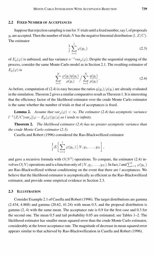
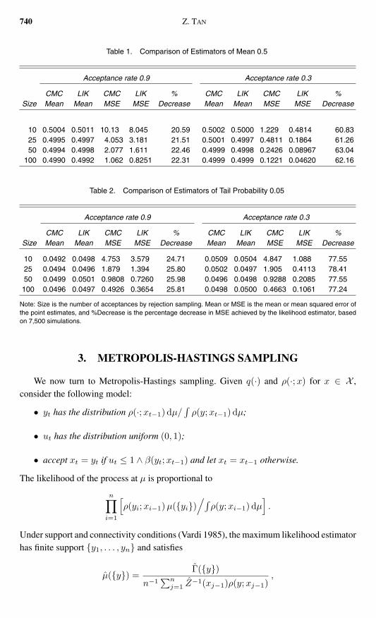
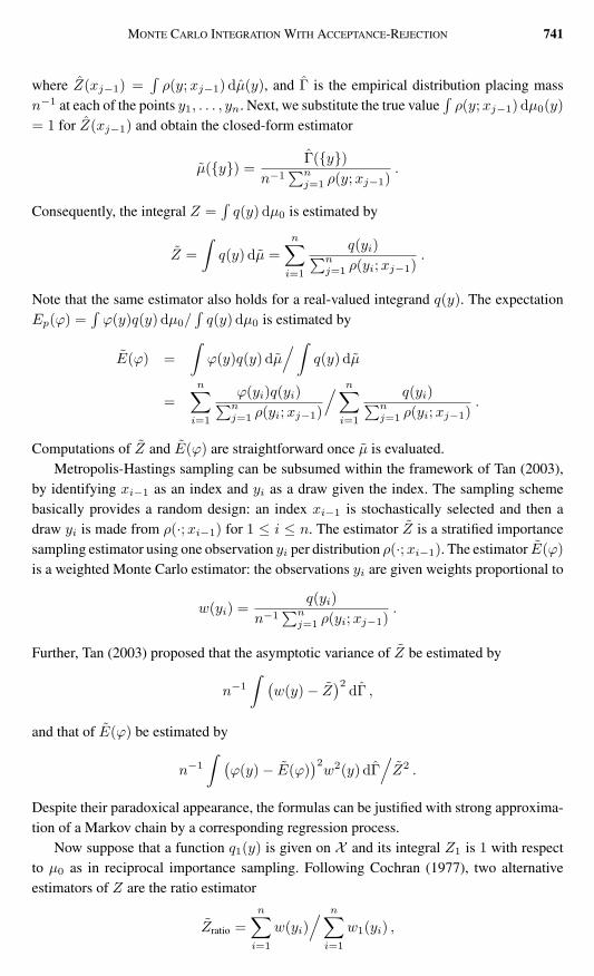
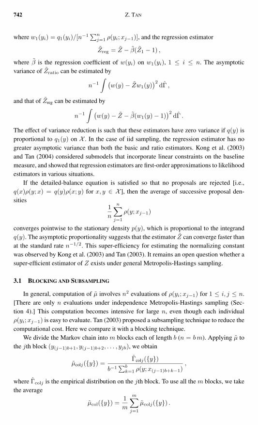
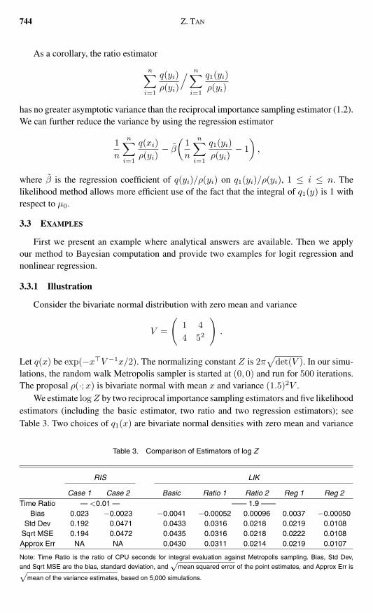
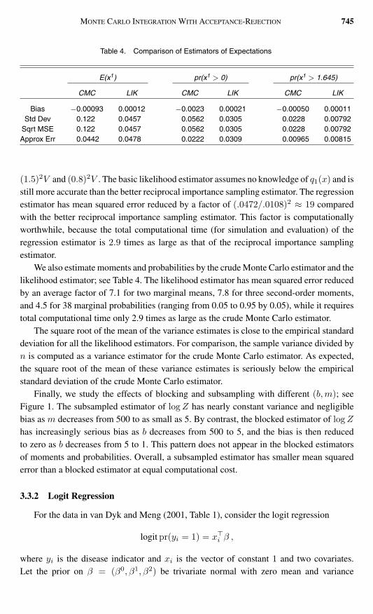
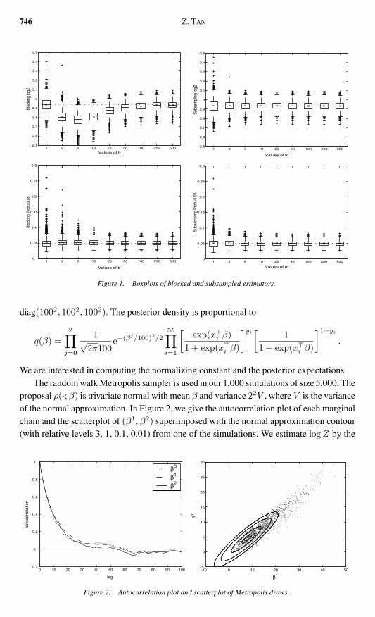
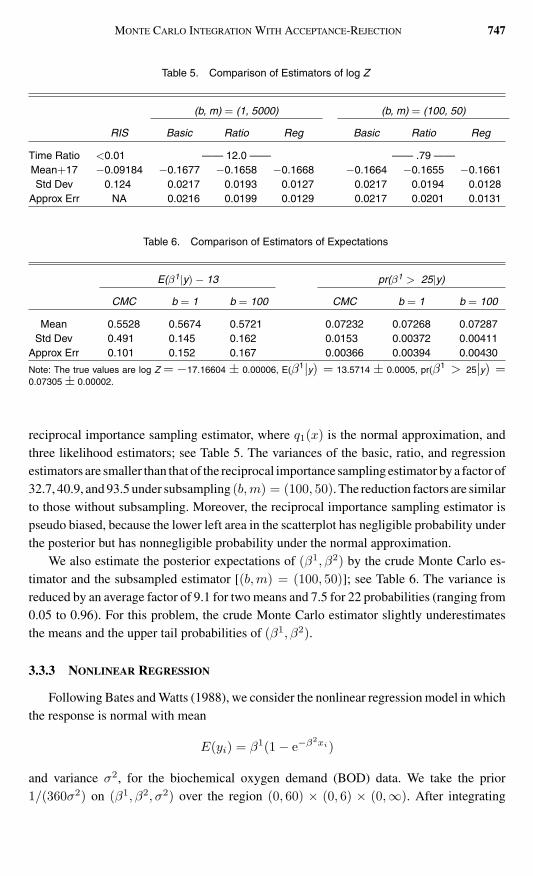
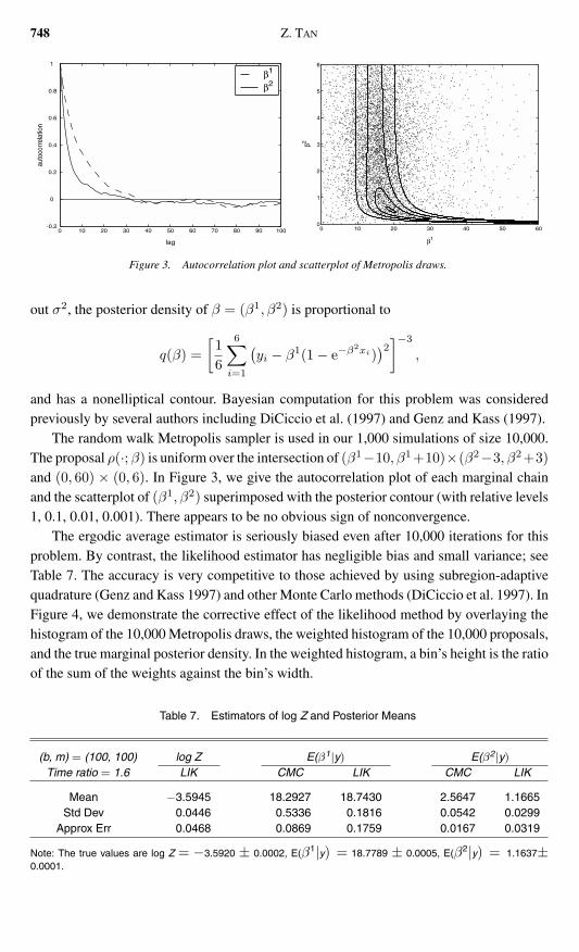
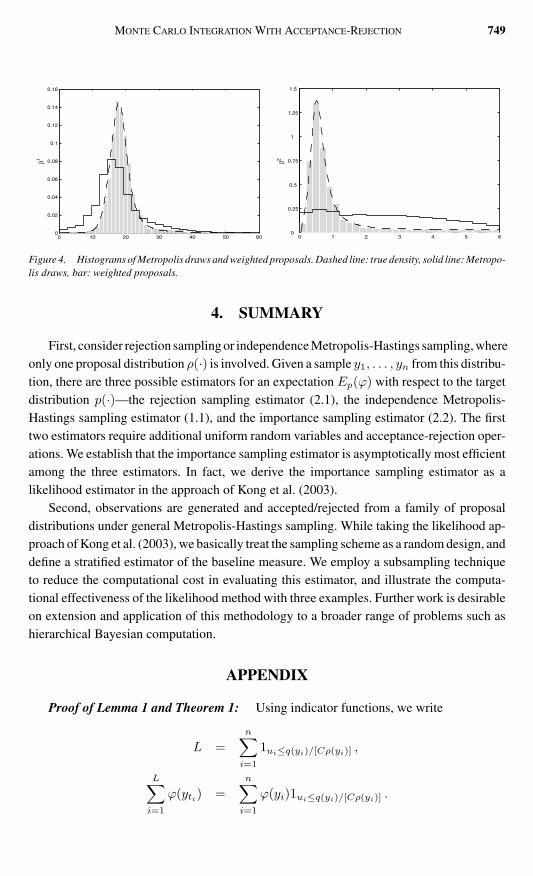
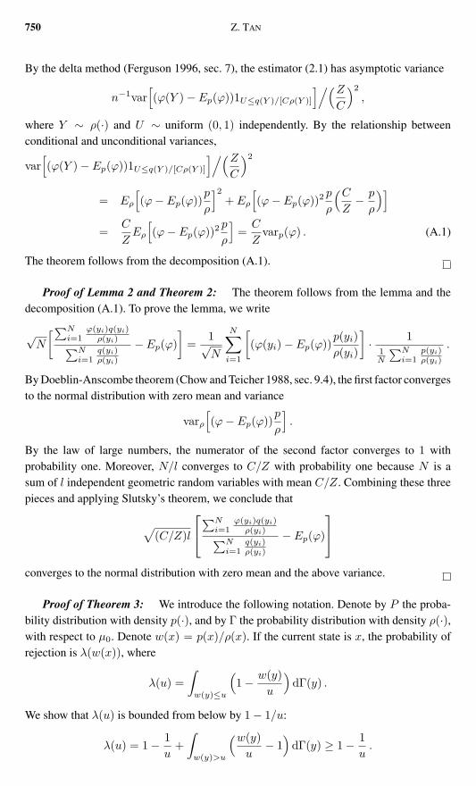736 Z TAN

sample average or the crude Monte Carlo (CMC) estimator

1n

nsumi=1

ϕ(xi) (11)

By letting ϕ(x) = q1(x)q(x) the normalizing constant Z can be estimated by(1n

nsumi=1

q1(xi)q(xi)

)minus1

(12)

where q1(x) is a probability density on X This estimator is called reciprocal importancesampling (RIS) see DiCiccio Kass Raftery and Wasserman (1997) and Gelfand and Dey(1994)

This article considers rejection sampling or Metropolis-Hastings sampling for the sim-ulation part Rejection sampling requires a probability density ρ(x) and a constant C suchthat q(x) le Cρ(x) on X which implies Z le C (von Neumann 1951) At each time t ge 1

bull Sample yt from ρ(middot)bull accept yt with probability q(yt)[Cρ(yt)] and move to the next trial otherwise

The second step can be implemented by generating ut from uniform (0 1) and acceptingyt if ut le q(yt)[Cρ(yt)] Then the accepted yt are independent and identically distributed(iid) as p(middot) To compare Metropolis-Hastings sampling requires a family of probabilitydensities ρ(middotx) x isin X (Metropolis et al 1953 Hastings 1970) At each time t ge 1

bull Sample yt from ρ(middotxtminus1)

bull accept xt = yt with probability 1 and β(ytxtminus1) and let xt = xtminus1 otherwise where

β(yx) =q(y)ρ(x y)q(x)ρ(yx)

The second step can also be implemented by generatingut from uniform (0 1) and acceptingxt = yt if ut le 1 and β(ytxtminus1) Under suitable regularity conditions the Markov chain(x1 x2 ) converges to the target distribution p(middot) In the so-called independence case(IMH) the proposal density ρ(middotx) equiv ρ(middot) is independent of x Then the chain is uniformlyergodic if q(x)ρ(x) is bounded from above on X and is not even geometrically ergodicotherwise (Mengersen and Tweedie 1996) The condition that q(x) le Cρ(x) on X isassumed henceforth

Neither rejection sampling nor Metropolis-Hastings sampling requires the value of thenormalizing constant Z However each algorithm involves accepting or rejecting obser-vations from proposal distributions Acceptance or rejection depends on uniform randomvariables By integrating out these uniform random variables Casella and Robert (1996)proposed a Rao-Blackwellized estimator that has no greater variance than the crude MonteCarlo estimator but they mostly disregarded the issue of computational time increased byRao-Blackwellization

Recently Kong et al (2003) formulated Monte Carlo integration as a statistical modelusing simulated observations as data The baseline measure is treated as the parameter and










1L

Lsumi=1

ϕ(yti) (21)




738 Z TAN







nprodi=1

[ρ(yi)micro(yi)

intρ(y) dmicro

]




intϕ(y)q(y) dmicro

intq(y) dmicro or

nsumi=1

ϕ(yi)q(yi)ρ(yi)

nsumi=1

q(yi)ρ(yi)

(22)





E

[L

n

∣∣ y1 yn

]=

1nC

nsumi=1

q(yi)ρ(yi)

E

[1n

Lsumi=1

ϕ(yti)∣∣ y1 yn

]=

1nC

nsumi=1

ϕ(yi)q(yi)ρ(yi)





1l

lsumi=1

ϕ(yti) (23)


Nsumi=1

ϕ(yi)q(yi)ρ(yi)

Nsumi=1

q(yi)ρ(yi)

(24)





1lE

[ lsumi=1


]


sumli=1 ϕ(yti)


23 ILLUSTRATION


740 Z TAN




10 05004 05011 1013 8045 2059 05002 05000 1229 04814 608325 04995 04997 4053 3181 2151 05001 04997 04811 01864 612650 04994 04998 2077 1611 2246 04999 04998 02426 008967 6304

100 04990 04992 1062 08251 2231 04999 04999 01221 004620 6216




10 00492 00498 4753 3579 2471 00509 00504 4847 1088 775525 00494 00496 1879 1394 2580 00502 00497 1905 04113 784150 00499 00501 09808 07260 2598 00496 00498 09288 02085 7755

100 00496 00497 04926 03654 2581 00498 00500 04663 01061 7724








nprodi=1



]



sumnj=1 Z









Z =intq(y) dmicro =

nsumi=1






intq(y) dmicro

=nsum

i=1


nsumi=1




w(yi) =q(yi)

nminus1sumn

j=1 ρ(yixjminus1)


nminus1int (


nminus1int (




Zratio =nsum

i=1

w(yi) nsum

i=1

w1(yi)

742 Z TAN




nminus1int (



nminus1int (




1n

nsumj=1

ρ(yxjminus1)








microcol(y) = 1m

msumj=1

microcolj(y)




where δyidenotes


1n

nsumi=1

q(yi)ρ(yiximinus1)






microrow(y) = 1b

bsumi=1

microrowi(y)



1m

msumk=1






744 Z TAN


nsumi=1

q(yi)ρ(yi)

nsumi=1

q1(yi)ρ(yi)


1n

nsumi=1

q(xi)ρ(yi)

minus β(1n

nsumi=1

q1(yi)ρ(yi)

minus 1)


33 EXAMPLES


331 Illustration


V =

(1 44 52

)





RIS LIK









E(x1) pr(x1 gt 0) pr(x1 gt 1645)












746 Z TAN



q(β) =2prod

j=0

1radic2π100


i=1

[exp(x

i β)1 + exp(x

i β)

]yi[

11 + exp(x

i β)

]1minusyi






(b m) = (1 5000) (b m) = (100 50)



Approx Err NA 00216 00199 00129 00217 00201 00131



CMC b = 1 b = 100 CMC b = 1 b = 100

Mean 05528 05674 05721 007232 007268 007287Std Dev 0491 0145 0162 00153 000372 000411

Approx Err 0101 0152 0167 000366 000394 000430








748 Z TAN



q(β) =[16

6sumi=1


)2]minus3







Approx Err 00468 00869 01759 00167 00319




4 SUMMARY



APPENDIX


L =nsum

i=1

1uileq(yi)[Cρ(yi)]

Lsumi=1

ϕ(yti) =nsum

i=1


750 Z TAN



](ZC

)2



](ZC

)2

= Eρ

[(ϕminus Ep(ϕ))

p

ρ

]2+ Eρ

[(ϕminus Ep(ϕ))2

p

ρ

(CZ

minus p

ρ

)]

=C

ZEρ

[(ϕminus Ep(ϕ))2

p

ρ

]=C

Zvarp(ϕ) (A1)



radicN

[sumNi=1


i=1q(yi)ρ(yi)

minus Ep(ϕ)]=

1radicN

Nsumi=1


p(yi)ρ(yi)

]middot 1

1N

sumNi=1

p(yi)ρ(yi)



p

ρ

]


radic(CZ)l

sumN

i=1ϕ(yi)q(yi)

ρ(yi)sumNi=1

q(yi)ρ(yi)

minus Ep(ϕ)



λ(u) =int

w(y)leu

(1 minus w(y)

u

)dΓ(y)



w(y)gtu

(w(y)u


u



int infin

u

kλkminus1(v)v2

dv





nminus1(γ0 + 2

infinsumk=1

γk

)


γk =intϕdagger(x)


]dP (x)

=intint



=intint


w(x)orw(y)

kλkminus1(u)u2 du

]dP (y) dP (x)

=intint


01ugew(x)1ugew(y)

kλkminus1(u)u2 du

]dP (y) dP (x)

=int infin

0

kλkminus1(u)u2



=int infin

0

kλkminus1(u)u2

[ int1ugew(x)ϕ

dagger(x) dP (x)]2

du ge 0


infinsumk=1


=intϕdagger2(x)


geintϕdagger2(x)




752 Z TAN

ACKNOWLEDGMENTS



REFERENCES





























1L

Lsumi=1

ϕ(yti) (21)




738 Z TAN







nprodi=1

[ρ(yi)micro(yi)

intρ(y) dmicro

]




intϕ(y)q(y) dmicro

intq(y) dmicro or

nsumi=1

ϕ(yi)q(yi)ρ(yi)

nsumi=1

q(yi)ρ(yi)

(22)





E

[L

n

∣∣ y1 yn

]=

1nC

nsumi=1

q(yi)ρ(yi)

E

[1n

Lsumi=1

ϕ(yti)∣∣ y1 yn

]=

1nC

nsumi=1

ϕ(yi)q(yi)ρ(yi)





1l

lsumi=1

ϕ(yti) (23)


Nsumi=1

ϕ(yi)q(yi)ρ(yi)

Nsumi=1

q(yi)ρ(yi)

(24)





1lE

[ lsumi=1


]


sumli=1 ϕ(yti)


23 ILLUSTRATION


740 Z TAN




10 05004 05011 1013 8045 2059 05002 05000 1229 04814 608325 04995 04997 4053 3181 2151 05001 04997 04811 01864 612650 04994 04998 2077 1611 2246 04999 04998 02426 008967 6304

100 04990 04992 1062 08251 2231 04999 04999 01221 004620 6216




10 00492 00498 4753 3579 2471 00509 00504 4847 1088 775525 00494 00496 1879 1394 2580 00502 00497 1905 04113 784150 00499 00501 09808 07260 2598 00496 00498 09288 02085 7755

100 00496 00497 04926 03654 2581 00498 00500 04663 01061 7724








nprodi=1



]



sumnj=1 Z









Z =intq(y) dmicro =

nsumi=1






intq(y) dmicro

=nsum

i=1


nsumi=1




w(yi) =q(yi)

nminus1sumn

j=1 ρ(yixjminus1)


nminus1int (


nminus1int (




Zratio =nsum

i=1

w(yi) nsum

i=1

w1(yi)

742 Z TAN




nminus1int (



nminus1int (




1n

nsumj=1

ρ(yxjminus1)








microcol(y) = 1m

msumj=1

microcolj(y)




where δyidenotes


1n

nsumi=1

q(yi)ρ(yiximinus1)






microrow(y) = 1b

bsumi=1

microrowi(y)



1m

msumk=1






744 Z TAN


nsumi=1

q(yi)ρ(yi)

nsumi=1

q1(yi)ρ(yi)


1n

nsumi=1

q(xi)ρ(yi)

minus β(1n

nsumi=1

q1(yi)ρ(yi)

minus 1)


33 EXAMPLES


331 Illustration


V =

(1 44 52

)





RIS LIK









E(x1) pr(x1 gt 0) pr(x1 gt 1645)












746 Z TAN



q(β) =2prod

j=0

1radic2π100


i=1

[exp(x

i β)1 + exp(x

i β)

]yi[

11 + exp(x

i β)

]1minusyi






(b m) = (1 5000) (b m) = (100 50)



Approx Err NA 00216 00199 00129 00217 00201 00131



CMC b = 1 b = 100 CMC b = 1 b = 100

Mean 05528 05674 05721 007232 007268 007287Std Dev 0491 0145 0162 00153 000372 000411

Approx Err 0101 0152 0167 000366 000394 000430








748 Z TAN



q(β) =[16

6sumi=1


)2]minus3







Approx Err 00468 00869 01759 00167 00319




4 SUMMARY



APPENDIX


L =nsum

i=1

1uileq(yi)[Cρ(yi)]

Lsumi=1

ϕ(yti) =nsum

i=1


750 Z TAN



](ZC

)2



](ZC

)2

= Eρ

[(ϕminus Ep(ϕ))

p

ρ

]2+ Eρ

[(ϕminus Ep(ϕ))2

p

ρ

(CZ

minus p

ρ

)]

=C

ZEρ

[(ϕminus Ep(ϕ))2

p

ρ

]=C

Zvarp(ϕ) (A1)



radicN

[sumNi=1


i=1q(yi)ρ(yi)

minus Ep(ϕ)]=

1radicN

Nsumi=1


p(yi)ρ(yi)

]middot 1

1N

sumNi=1

p(yi)ρ(yi)



p

ρ

]


radic(CZ)l

sumN

i=1ϕ(yi)q(yi)

ρ(yi)sumNi=1

q(yi)ρ(yi)

minus Ep(ϕ)



λ(u) =int

w(y)leu

(1 minus w(y)

u

)dΓ(y)



w(y)gtu

(w(y)u


u



int infin

u

kλkminus1(v)v2

dv





nminus1(γ0 + 2

infinsumk=1

γk

)


γk =intϕdagger(x)


]dP (x)

=intint



=intint


w(x)orw(y)

kλkminus1(u)u2 du

]dP (y) dP (x)

=intint


01ugew(x)1ugew(y)

kλkminus1(u)u2 du

]dP (y) dP (x)

=int infin

0

kλkminus1(u)u2



=int infin

0

kλkminus1(u)u2

[ int1ugew(x)ϕ

dagger(x) dP (x)]2

du ge 0


infinsumk=1


=intϕdagger2(x)


geintϕdagger2(x)




752 Z TAN

ACKNOWLEDGMENTS



REFERENCES




















738 Z TAN







nprodi=1

[ρ(yi)micro(yi)

intρ(y) dmicro

]




intϕ(y)q(y) dmicro

intq(y) dmicro or

nsumi=1

ϕ(yi)q(yi)ρ(yi)

nsumi=1

q(yi)ρ(yi)

(22)





E

[L

n

∣∣ y1 yn

]=

1nC

nsumi=1

q(yi)ρ(yi)

E

[1n

Lsumi=1

ϕ(yti)∣∣ y1 yn

]=

1nC

nsumi=1

ϕ(yi)q(yi)ρ(yi)





1l

lsumi=1

ϕ(yti) (23)


Nsumi=1

ϕ(yi)q(yi)ρ(yi)

Nsumi=1

q(yi)ρ(yi)

(24)





1lE

[ lsumi=1


]


sumli=1 ϕ(yti)


23 ILLUSTRATION


740 Z TAN




10 05004 05011 1013 8045 2059 05002 05000 1229 04814 608325 04995 04997 4053 3181 2151 05001 04997 04811 01864 612650 04994 04998 2077 1611 2246 04999 04998 02426 008967 6304

100 04990 04992 1062 08251 2231 04999 04999 01221 004620 6216




10 00492 00498 4753 3579 2471 00509 00504 4847 1088 775525 00494 00496 1879 1394 2580 00502 00497 1905 04113 784150 00499 00501 09808 07260 2598 00496 00498 09288 02085 7755

100 00496 00497 04926 03654 2581 00498 00500 04663 01061 7724








nprodi=1



]



sumnj=1 Z









Z =intq(y) dmicro =

nsumi=1






intq(y) dmicro

=nsum

i=1


nsumi=1




w(yi) =q(yi)

nminus1sumn

j=1 ρ(yixjminus1)


nminus1int (


nminus1int (




Zratio =nsum

i=1

w(yi) nsum

i=1

w1(yi)

742 Z TAN




nminus1int (



nminus1int (




1n

nsumj=1

ρ(yxjminus1)








microcol(y) = 1m

msumj=1

microcolj(y)




where δyidenotes


1n

nsumi=1

q(yi)ρ(yiximinus1)






microrow(y) = 1b

bsumi=1

microrowi(y)



1m

msumk=1






744 Z TAN


nsumi=1

q(yi)ρ(yi)

nsumi=1

q1(yi)ρ(yi)


1n

nsumi=1

q(xi)ρ(yi)

minus β(1n

nsumi=1

q1(yi)ρ(yi)

minus 1)


33 EXAMPLES


331 Illustration


V =

(1 44 52

)





RIS LIK









E(x1) pr(x1 gt 0) pr(x1 gt 1645)












746 Z TAN



q(β) =2prod

j=0

1radic2π100


i=1

[exp(x

i β)1 + exp(x

i β)

]yi[

11 + exp(x

i β)

]1minusyi






(b m) = (1 5000) (b m) = (100 50)



Approx Err NA 00216 00199 00129 00217 00201 00131



CMC b = 1 b = 100 CMC b = 1 b = 100

Mean 05528 05674 05721 007232 007268 007287Std Dev 0491 0145 0162 00153 000372 000411

Approx Err 0101 0152 0167 000366 000394 000430








748 Z TAN



q(β) =[16

6sumi=1


)2]minus3







Approx Err 00468 00869 01759 00167 00319




4 SUMMARY



APPENDIX


L =nsum

i=1

1uileq(yi)[Cρ(yi)]

Lsumi=1

ϕ(yti) =nsum

i=1


750 Z TAN



](ZC

)2



](ZC

)2

= Eρ

[(ϕminus Ep(ϕ))

p

ρ

]2+ Eρ

[(ϕminus Ep(ϕ))2

p

ρ

(CZ

minus p

ρ

)]

=C

ZEρ

[(ϕminus Ep(ϕ))2

p

ρ

]=C

Zvarp(ϕ) (A1)



radicN

[sumNi=1


i=1q(yi)ρ(yi)

minus Ep(ϕ)]=

1radicN

Nsumi=1


p(yi)ρ(yi)

]middot 1

1N

sumNi=1

p(yi)ρ(yi)



p

ρ

]


radic(CZ)l

sumN

i=1ϕ(yi)q(yi)

ρ(yi)sumNi=1

q(yi)ρ(yi)

minus Ep(ϕ)



λ(u) =int

w(y)leu

(1 minus w(y)

u

)dΓ(y)



w(y)gtu

(w(y)u


u



int infin

u

kλkminus1(v)v2

dv





nminus1(γ0 + 2

infinsumk=1

γk

)


γk =intϕdagger(x)


]dP (x)

=intint



=intint


w(x)orw(y)

kλkminus1(u)u2 du

]dP (y) dP (x)

=intint


01ugew(x)1ugew(y)

kλkminus1(u)u2 du

]dP (y) dP (x)

=int infin

0

kλkminus1(u)u2



=int infin

0

kλkminus1(u)u2

[ int1ugew(x)ϕ

dagger(x) dP (x)]2

du ge 0


infinsumk=1


=intϕdagger2(x)


geintϕdagger2(x)




752 Z TAN

ACKNOWLEDGMENTS



REFERENCES























1l

lsumi=1

ϕ(yti) (23)


Nsumi=1

ϕ(yi)q(yi)ρ(yi)

Nsumi=1

q(yi)ρ(yi)

(24)





1lE

[ lsumi=1


]


sumli=1 ϕ(yti)


23 ILLUSTRATION


740 Z TAN




10 05004 05011 1013 8045 2059 05002 05000 1229 04814 608325 04995 04997 4053 3181 2151 05001 04997 04811 01864 612650 04994 04998 2077 1611 2246 04999 04998 02426 008967 6304

100 04990 04992 1062 08251 2231 04999 04999 01221 004620 6216




10 00492 00498 4753 3579 2471 00509 00504 4847 1088 775525 00494 00496 1879 1394 2580 00502 00497 1905 04113 784150 00499 00501 09808 07260 2598 00496 00498 09288 02085 7755

100 00496 00497 04926 03654 2581 00498 00500 04663 01061 7724








nprodi=1



]



sumnj=1 Z









Z =intq(y) dmicro =

nsumi=1






intq(y) dmicro

=nsum

i=1


nsumi=1




w(yi) =q(yi)

nminus1sumn

j=1 ρ(yixjminus1)


nminus1int (


nminus1int (




Zratio =nsum

i=1

w(yi) nsum

i=1

w1(yi)

742 Z TAN




nminus1int (



nminus1int (




1n

nsumj=1

ρ(yxjminus1)








microcol(y) = 1m

msumj=1

microcolj(y)




where δyidenotes


1n

nsumi=1

q(yi)ρ(yiximinus1)






microrow(y) = 1b

bsumi=1

microrowi(y)



1m

msumk=1






744 Z TAN


nsumi=1

q(yi)ρ(yi)

nsumi=1

q1(yi)ρ(yi)


1n

nsumi=1

q(xi)ρ(yi)

minus β(1n

nsumi=1

q1(yi)ρ(yi)

minus 1)


33 EXAMPLES


331 Illustration


V =

(1 44 52

)





RIS LIK









E(x1) pr(x1 gt 0) pr(x1 gt 1645)












746 Z TAN



q(β) =2prod

j=0

1radic2π100


i=1

[exp(x

i β)1 + exp(x

i β)

]yi[

11 + exp(x

i β)

]1minusyi






(b m) = (1 5000) (b m) = (100 50)



Approx Err NA 00216 00199 00129 00217 00201 00131



CMC b = 1 b = 100 CMC b = 1 b = 100

Mean 05528 05674 05721 007232 007268 007287Std Dev 0491 0145 0162 00153 000372 000411

Approx Err 0101 0152 0167 000366 000394 000430








748 Z TAN



q(β) =[16

6sumi=1


)2]minus3







Approx Err 00468 00869 01759 00167 00319




4 SUMMARY



APPENDIX


L =nsum

i=1

1uileq(yi)[Cρ(yi)]

Lsumi=1

ϕ(yti) =nsum

i=1


750 Z TAN



](ZC

)2



](ZC

)2

= Eρ

[(ϕminus Ep(ϕ))

p

ρ

]2+ Eρ

[(ϕminus Ep(ϕ))2

p

ρ

(CZ

minus p

ρ

)]

=C

ZEρ

[(ϕminus Ep(ϕ))2

p

ρ

]=C

Zvarp(ϕ) (A1)



radicN

[sumNi=1


i=1q(yi)ρ(yi)

minus Ep(ϕ)]=

1radicN

Nsumi=1


p(yi)ρ(yi)

]middot 1

1N

sumNi=1

p(yi)ρ(yi)



p

ρ

]


radic(CZ)l

sumN

i=1ϕ(yi)q(yi)

ρ(yi)sumNi=1

q(yi)ρ(yi)

minus Ep(ϕ)



λ(u) =int

w(y)leu

(1 minus w(y)

u

)dΓ(y)



w(y)gtu

(w(y)u


u



int infin

u

kλkminus1(v)v2

dv





nminus1(γ0 + 2

infinsumk=1

γk

)


γk =intϕdagger(x)


]dP (x)

=intint



=intint


w(x)orw(y)

kλkminus1(u)u2 du

]dP (y) dP (x)

=intint


01ugew(x)1ugew(y)

kλkminus1(u)u2 du

]dP (y) dP (x)

=int infin

0

kλkminus1(u)u2



=int infin

0

kλkminus1(u)u2

[ int1ugew(x)ϕ

dagger(x) dP (x)]2

du ge 0


infinsumk=1


=intϕdagger2(x)


geintϕdagger2(x)




752 Z TAN

ACKNOWLEDGMENTS



REFERENCES




















740 Z TAN




10 05004 05011 1013 8045 2059 05002 05000 1229 04814 608325 04995 04997 4053 3181 2151 05001 04997 04811 01864 612650 04994 04998 2077 1611 2246 04999 04998 02426 008967 6304

100 04990 04992 1062 08251 2231 04999 04999 01221 004620 6216




10 00492 00498 4753 3579 2471 00509 00504 4847 1088 775525 00494 00496 1879 1394 2580 00502 00497 1905 04113 784150 00499 00501 09808 07260 2598 00496 00498 09288 02085 7755

100 00496 00497 04926 03654 2581 00498 00500 04663 01061 7724








nprodi=1



]



sumnj=1 Z









Z =intq(y) dmicro =

nsumi=1






intq(y) dmicro

=nsum

i=1


nsumi=1




w(yi) =q(yi)

nminus1sumn

j=1 ρ(yixjminus1)


nminus1int (


nminus1int (




Zratio =nsum

i=1

w(yi) nsum

i=1

w1(yi)

742 Z TAN




nminus1int (



nminus1int (




1n

nsumj=1

ρ(yxjminus1)








microcol(y) = 1m

msumj=1

microcolj(y)




where δyidenotes


1n

nsumi=1

q(yi)ρ(yiximinus1)






microrow(y) = 1b

bsumi=1

microrowi(y)



1m

msumk=1






744 Z TAN


nsumi=1

q(yi)ρ(yi)

nsumi=1

q1(yi)ρ(yi)


1n

nsumi=1

q(xi)ρ(yi)

minus β(1n

nsumi=1

q1(yi)ρ(yi)

minus 1)


33 EXAMPLES


331 Illustration


V =

(1 44 52

)





RIS LIK









E(x1) pr(x1 gt 0) pr(x1 gt 1645)












746 Z TAN



q(β) =2prod

j=0

1radic2π100


i=1

[exp(x

i β)1 + exp(x

i β)

]yi[

11 + exp(x

i β)

]1minusyi






(b m) = (1 5000) (b m) = (100 50)



Approx Err NA 00216 00199 00129 00217 00201 00131



CMC b = 1 b = 100 CMC b = 1 b = 100

Mean 05528 05674 05721 007232 007268 007287Std Dev 0491 0145 0162 00153 000372 000411

Approx Err 0101 0152 0167 000366 000394 000430








748 Z TAN



q(β) =[16

6sumi=1


)2]minus3







Approx Err 00468 00869 01759 00167 00319




4 SUMMARY



APPENDIX


L =nsum

i=1

1uileq(yi)[Cρ(yi)]

Lsumi=1

ϕ(yti) =nsum

i=1


750 Z TAN



](ZC

)2



](ZC

)2

= Eρ

[(ϕminus Ep(ϕ))

p

ρ

]2+ Eρ

[(ϕminus Ep(ϕ))2

p

ρ

(CZ

minus p

ρ

)]

=C

ZEρ

[(ϕminus Ep(ϕ))2

p

ρ

]=C

Zvarp(ϕ) (A1)



radicN

[sumNi=1


i=1q(yi)ρ(yi)

minus Ep(ϕ)]=

1radicN

Nsumi=1


p(yi)ρ(yi)

]middot 1

1N

sumNi=1

p(yi)ρ(yi)



p

ρ

]


radic(CZ)l

sumN

i=1ϕ(yi)q(yi)

ρ(yi)sumNi=1

q(yi)ρ(yi)

minus Ep(ϕ)



λ(u) =int

w(y)leu

(1 minus w(y)

u

)dΓ(y)



w(y)gtu

(w(y)u


u



int infin

u

kλkminus1(v)v2

dv





nminus1(γ0 + 2

infinsumk=1

γk

)


γk =intϕdagger(x)


]dP (x)

=intint



=intint


w(x)orw(y)

kλkminus1(u)u2 du

]dP (y) dP (x)

=intint


01ugew(x)1ugew(y)

kλkminus1(u)u2 du

]dP (y) dP (x)

=int infin

0

kλkminus1(u)u2



=int infin

0

kλkminus1(u)u2

[ int1ugew(x)ϕ

dagger(x) dP (x)]2

du ge 0


infinsumk=1


=intϕdagger2(x)


geintϕdagger2(x)




752 Z TAN

ACKNOWLEDGMENTS



REFERENCES



























Z =intq(y) dmicro =

nsumi=1






intq(y) dmicro

=nsum

i=1


nsumi=1




w(yi) =q(yi)

nminus1sumn

j=1 ρ(yixjminus1)


nminus1int (


nminus1int (




Zratio =nsum

i=1

w(yi) nsum

i=1

w1(yi)

742 Z TAN




nminus1int (



nminus1int (




1n

nsumj=1

ρ(yxjminus1)








microcol(y) = 1m

msumj=1

microcolj(y)




where δyidenotes


1n

nsumi=1

q(yi)ρ(yiximinus1)






microrow(y) = 1b

bsumi=1

microrowi(y)



1m

msumk=1






744 Z TAN


nsumi=1

q(yi)ρ(yi)

nsumi=1

q1(yi)ρ(yi)


1n

nsumi=1

q(xi)ρ(yi)

minus β(1n

nsumi=1

q1(yi)ρ(yi)

minus 1)


33 EXAMPLES


331 Illustration


V =

(1 44 52

)





RIS LIK









E(x1) pr(x1 gt 0) pr(x1 gt 1645)












746 Z TAN



q(β) =2prod

j=0

1radic2π100


i=1

[exp(x

i β)1 + exp(x

i β)

]yi[

11 + exp(x

i β)

]1minusyi






(b m) = (1 5000) (b m) = (100 50)



Approx Err NA 00216 00199 00129 00217 00201 00131



CMC b = 1 b = 100 CMC b = 1 b = 100

Mean 05528 05674 05721 007232 007268 007287Std Dev 0491 0145 0162 00153 000372 000411

Approx Err 0101 0152 0167 000366 000394 000430








748 Z TAN



q(β) =[16

6sumi=1


)2]minus3







Approx Err 00468 00869 01759 00167 00319




4 SUMMARY



APPENDIX


L =nsum

i=1

1uileq(yi)[Cρ(yi)]

Lsumi=1

ϕ(yti) =nsum

i=1


750 Z TAN



](ZC

)2



](ZC

)2

= Eρ

[(ϕminus Ep(ϕ))

p

ρ

]2+ Eρ

[(ϕminus Ep(ϕ))2

p

ρ

(CZ

minus p

ρ

)]

=C

ZEρ

[(ϕminus Ep(ϕ))2

p

ρ

]=C

Zvarp(ϕ) (A1)



radicN

[sumNi=1


i=1q(yi)ρ(yi)

minus Ep(ϕ)]=

1radicN

Nsumi=1


p(yi)ρ(yi)

]middot 1

1N

sumNi=1

p(yi)ρ(yi)



p

ρ

]


radic(CZ)l

sumN

i=1ϕ(yi)q(yi)

ρ(yi)sumNi=1

q(yi)ρ(yi)

minus Ep(ϕ)



λ(u) =int

w(y)leu

(1 minus w(y)

u

)dΓ(y)



w(y)gtu

(w(y)u


u



int infin

u

kλkminus1(v)v2

dv





nminus1(γ0 + 2

infinsumk=1

γk

)


γk =intϕdagger(x)


]dP (x)

=intint



=intint


w(x)orw(y)

kλkminus1(u)u2 du

]dP (y) dP (x)

=intint


01ugew(x)1ugew(y)

kλkminus1(u)u2 du

]dP (y) dP (x)

=int infin

0

kλkminus1(u)u2



=int infin

0

kλkminus1(u)u2

[ int1ugew(x)ϕ

dagger(x) dP (x)]2

du ge 0


infinsumk=1


=intϕdagger2(x)


geintϕdagger2(x)




752 Z TAN

ACKNOWLEDGMENTS



REFERENCES




















742 Z TAN




nminus1int (



nminus1int (




1n

nsumj=1

ρ(yxjminus1)








microcol(y) = 1m

msumj=1

microcolj(y)




where δyidenotes


1n

nsumi=1

q(yi)ρ(yiximinus1)






microrow(y) = 1b

bsumi=1

microrowi(y)



1m

msumk=1






744 Z TAN


nsumi=1

q(yi)ρ(yi)

nsumi=1

q1(yi)ρ(yi)


1n

nsumi=1

q(xi)ρ(yi)

minus β(1n

nsumi=1

q1(yi)ρ(yi)

minus 1)


33 EXAMPLES


331 Illustration


V =

(1 44 52

)





RIS LIK









E(x1) pr(x1 gt 0) pr(x1 gt 1645)












746 Z TAN



q(β) =2prod

j=0

1radic2π100


i=1

[exp(x

i β)1 + exp(x

i β)

]yi[

11 + exp(x

i β)

]1minusyi






(b m) = (1 5000) (b m) = (100 50)



Approx Err NA 00216 00199 00129 00217 00201 00131



CMC b = 1 b = 100 CMC b = 1 b = 100

Mean 05528 05674 05721 007232 007268 007287Std Dev 0491 0145 0162 00153 000372 000411

Approx Err 0101 0152 0167 000366 000394 000430








748 Z TAN



q(β) =[16

6sumi=1


)2]minus3







Approx Err 00468 00869 01759 00167 00319




4 SUMMARY



APPENDIX


L =nsum

i=1

1uileq(yi)[Cρ(yi)]

Lsumi=1

ϕ(yti) =nsum

i=1


750 Z TAN



](ZC

)2



](ZC

)2

= Eρ

[(ϕminus Ep(ϕ))

p

ρ

]2+ Eρ

[(ϕminus Ep(ϕ))2

p

ρ

(CZ

minus p

ρ

)]

=C

ZEρ

[(ϕminus Ep(ϕ))2

p

ρ

]=C

Zvarp(ϕ) (A1)



radicN

[sumNi=1


i=1q(yi)ρ(yi)

minus Ep(ϕ)]=

1radicN

Nsumi=1


p(yi)ρ(yi)

]middot 1

1N

sumNi=1

p(yi)ρ(yi)



p

ρ

]


radic(CZ)l

sumN

i=1ϕ(yi)q(yi)

ρ(yi)sumNi=1

q(yi)ρ(yi)

minus Ep(ϕ)



λ(u) =int

w(y)leu

(1 minus w(y)

u

)dΓ(y)



w(y)gtu

(w(y)u


u



int infin

u

kλkminus1(v)v2

dv





nminus1(γ0 + 2

infinsumk=1

γk

)


γk =intϕdagger(x)


]dP (x)

=intint



=intint


w(x)orw(y)

kλkminus1(u)u2 du

]dP (y) dP (x)

=intint


01ugew(x)1ugew(y)

kλkminus1(u)u2 du

]dP (y) dP (x)

=int infin

0

kλkminus1(u)u2



=int infin

0

kλkminus1(u)u2

[ int1ugew(x)ϕ

dagger(x) dP (x)]2

du ge 0


infinsumk=1


=intϕdagger2(x)


geintϕdagger2(x)




752 Z TAN

ACKNOWLEDGMENTS



REFERENCES























where δyidenotes


1n

nsumi=1

q(yi)ρ(yiximinus1)






microrow(y) = 1b

bsumi=1

microrowi(y)



1m

msumk=1






744 Z TAN


nsumi=1

q(yi)ρ(yi)

nsumi=1

q1(yi)ρ(yi)


1n

nsumi=1

q(xi)ρ(yi)

minus β(1n

nsumi=1

q1(yi)ρ(yi)

minus 1)


33 EXAMPLES


331 Illustration


V =

(1 44 52

)





RIS LIK









E(x1) pr(x1 gt 0) pr(x1 gt 1645)












746 Z TAN



q(β) =2prod

j=0

1radic2π100


i=1

[exp(x

i β)1 + exp(x

i β)

]yi[

11 + exp(x

i β)

]1minusyi






(b m) = (1 5000) (b m) = (100 50)



Approx Err NA 00216 00199 00129 00217 00201 00131



CMC b = 1 b = 100 CMC b = 1 b = 100

Mean 05528 05674 05721 007232 007268 007287Std Dev 0491 0145 0162 00153 000372 000411

Approx Err 0101 0152 0167 000366 000394 000430








748 Z TAN



q(β) =[16

6sumi=1


)2]minus3







Approx Err 00468 00869 01759 00167 00319




4 SUMMARY



APPENDIX


L =nsum

i=1

1uileq(yi)[Cρ(yi)]

Lsumi=1

ϕ(yti) =nsum

i=1


750 Z TAN



](ZC

)2



](ZC

)2

= Eρ

[(ϕminus Ep(ϕ))

p

ρ

]2+ Eρ

[(ϕminus Ep(ϕ))2

p

ρ

(CZ

minus p

ρ

)]

=C

ZEρ

[(ϕminus Ep(ϕ))2

p

ρ

]=C

Zvarp(ϕ) (A1)



radicN

[sumNi=1


i=1q(yi)ρ(yi)

minus Ep(ϕ)]=

1radicN

Nsumi=1


p(yi)ρ(yi)

]middot 1

1N

sumNi=1

p(yi)ρ(yi)



p

ρ

]


radic(CZ)l

sumN

i=1ϕ(yi)q(yi)

ρ(yi)sumNi=1

q(yi)ρ(yi)

minus Ep(ϕ)



λ(u) =int

w(y)leu

(1 minus w(y)

u

)dΓ(y)



w(y)gtu

(w(y)u


u



int infin

u

kλkminus1(v)v2

dv





nminus1(γ0 + 2

infinsumk=1

γk

)


γk =intϕdagger(x)


]dP (x)

=intint



=intint


w(x)orw(y)

kλkminus1(u)u2 du

]dP (y) dP (x)

=intint


01ugew(x)1ugew(y)

kλkminus1(u)u2 du

]dP (y) dP (x)

=int infin

0

kλkminus1(u)u2



=int infin

0

kλkminus1(u)u2

[ int1ugew(x)ϕ

dagger(x) dP (x)]2

du ge 0


infinsumk=1


=intϕdagger2(x)


geintϕdagger2(x)




752 Z TAN

ACKNOWLEDGMENTS



REFERENCES




















744 Z TAN


nsumi=1

q(yi)ρ(yi)

nsumi=1

q1(yi)ρ(yi)


1n

nsumi=1

q(xi)ρ(yi)

minus β(1n

nsumi=1

q1(yi)ρ(yi)

minus 1)


33 EXAMPLES


331 Illustration


V =

(1 44 52

)





RIS LIK









E(x1) pr(x1 gt 0) pr(x1 gt 1645)












746 Z TAN



q(β) =2prod

j=0

1radic2π100


i=1

[exp(x

i β)1 + exp(x

i β)

]yi[

11 + exp(x

i β)

]1minusyi






(b m) = (1 5000) (b m) = (100 50)



Approx Err NA 00216 00199 00129 00217 00201 00131



CMC b = 1 b = 100 CMC b = 1 b = 100

Mean 05528 05674 05721 007232 007268 007287Std Dev 0491 0145 0162 00153 000372 000411

Approx Err 0101 0152 0167 000366 000394 000430








748 Z TAN



q(β) =[16

6sumi=1


)2]minus3







Approx Err 00468 00869 01759 00167 00319




4 SUMMARY



APPENDIX


L =nsum

i=1

1uileq(yi)[Cρ(yi)]

Lsumi=1

ϕ(yti) =nsum

i=1


750 Z TAN



](ZC

)2



](ZC

)2

= Eρ

[(ϕminus Ep(ϕ))

p

ρ

]2+ Eρ

[(ϕminus Ep(ϕ))2

p

ρ

(CZ

minus p

ρ

)]

=C

ZEρ

[(ϕminus Ep(ϕ))2

p

ρ

]=C

Zvarp(ϕ) (A1)



radicN

[sumNi=1


i=1q(yi)ρ(yi)

minus Ep(ϕ)]=

1radicN

Nsumi=1


p(yi)ρ(yi)

]middot 1

1N

sumNi=1

p(yi)ρ(yi)



p

ρ

]


radic(CZ)l

sumN

i=1ϕ(yi)q(yi)

ρ(yi)sumNi=1

q(yi)ρ(yi)

minus Ep(ϕ)



λ(u) =int

w(y)leu

(1 minus w(y)

u

)dΓ(y)



w(y)gtu

(w(y)u


u



int infin

u

kλkminus1(v)v2

dv





nminus1(γ0 + 2

infinsumk=1

γk

)


γk =intϕdagger(x)


]dP (x)

=intint



=intint


w(x)orw(y)

kλkminus1(u)u2 du

]dP (y) dP (x)

=intint


01ugew(x)1ugew(y)

kλkminus1(u)u2 du

]dP (y) dP (x)

=int infin

0

kλkminus1(u)u2



=int infin

0

kλkminus1(u)u2

[ int1ugew(x)ϕ

dagger(x) dP (x)]2

du ge 0


infinsumk=1


=intϕdagger2(x)


geintϕdagger2(x)




752 Z TAN

ACKNOWLEDGMENTS



REFERENCES






















E(x1) pr(x1 gt 0) pr(x1 gt 1645)












746 Z TAN



q(β) =2prod

j=0

1radic2π100


i=1

[exp(x

i β)1 + exp(x

i β)

]yi[

11 + exp(x

i β)

]1minusyi






(b m) = (1 5000) (b m) = (100 50)



Approx Err NA 00216 00199 00129 00217 00201 00131



CMC b = 1 b = 100 CMC b = 1 b = 100

Mean 05528 05674 05721 007232 007268 007287Std Dev 0491 0145 0162 00153 000372 000411

Approx Err 0101 0152 0167 000366 000394 000430








748 Z TAN



q(β) =[16

6sumi=1


)2]minus3







Approx Err 00468 00869 01759 00167 00319




4 SUMMARY



APPENDIX


L =nsum

i=1

1uileq(yi)[Cρ(yi)]

Lsumi=1

ϕ(yti) =nsum

i=1


750 Z TAN



](ZC

)2



](ZC

)2

= Eρ

[(ϕminus Ep(ϕ))

p

ρ

]2+ Eρ

[(ϕminus Ep(ϕ))2

p

ρ

(CZ

minus p

ρ

)]

=C

ZEρ

[(ϕminus Ep(ϕ))2

p

ρ

]=C

Zvarp(ϕ) (A1)



radicN

[sumNi=1


i=1q(yi)ρ(yi)

minus Ep(ϕ)]=

1radicN

Nsumi=1


p(yi)ρ(yi)

]middot 1

1N

sumNi=1

p(yi)ρ(yi)



p

ρ

]


radic(CZ)l

sumN

i=1ϕ(yi)q(yi)

ρ(yi)sumNi=1

q(yi)ρ(yi)

minus Ep(ϕ)



λ(u) =int

w(y)leu

(1 minus w(y)

u

)dΓ(y)



w(y)gtu

(w(y)u


u



int infin

u

kλkminus1(v)v2

dv





nminus1(γ0 + 2

infinsumk=1

γk

)


γk =intϕdagger(x)


]dP (x)

=intint



=intint


w(x)orw(y)

kλkminus1(u)u2 du

]dP (y) dP (x)

=intint


01ugew(x)1ugew(y)

kλkminus1(u)u2 du

]dP (y) dP (x)

=int infin

0

kλkminus1(u)u2



=int infin

0

kλkminus1(u)u2

[ int1ugew(x)ϕ

dagger(x) dP (x)]2

du ge 0


infinsumk=1


=intϕdagger2(x)


geintϕdagger2(x)




752 Z TAN

ACKNOWLEDGMENTS



REFERENCES




















746 Z TAN



q(β) =2prod

j=0

1radic2π100


i=1

[exp(x

i β)1 + exp(x

i β)

]yi[

11 + exp(x

i β)

]1minusyi






(b m) = (1 5000) (b m) = (100 50)



Approx Err NA 00216 00199 00129 00217 00201 00131



CMC b = 1 b = 100 CMC b = 1 b = 100

Mean 05528 05674 05721 007232 007268 007287Std Dev 0491 0145 0162 00153 000372 000411

Approx Err 0101 0152 0167 000366 000394 000430








748 Z TAN



q(β) =[16

6sumi=1


)2]minus3







Approx Err 00468 00869 01759 00167 00319




4 SUMMARY



APPENDIX


L =nsum

i=1

1uileq(yi)[Cρ(yi)]

Lsumi=1

ϕ(yti) =nsum

i=1


750 Z TAN



](ZC

)2



](ZC

)2

= Eρ

[(ϕminus Ep(ϕ))

p

ρ

]2+ Eρ

[(ϕminus Ep(ϕ))2

p

ρ

(CZ

minus p

ρ

)]

=C

ZEρ

[(ϕminus Ep(ϕ))2

p

ρ

]=C

Zvarp(ϕ) (A1)



radicN

[sumNi=1


i=1q(yi)ρ(yi)

minus Ep(ϕ)]=

1radicN

Nsumi=1


p(yi)ρ(yi)

]middot 1

1N

sumNi=1

p(yi)ρ(yi)



p

ρ

]


radic(CZ)l

sumN

i=1ϕ(yi)q(yi)

ρ(yi)sumNi=1

q(yi)ρ(yi)

minus Ep(ϕ)



λ(u) =int

w(y)leu

(1 minus w(y)

u

)dΓ(y)



w(y)gtu

(w(y)u


u



int infin

u

kλkminus1(v)v2

dv





nminus1(γ0 + 2

infinsumk=1

γk

)


γk =intϕdagger(x)


]dP (x)

=intint



=intint


w(x)orw(y)

kλkminus1(u)u2 du

]dP (y) dP (x)

=intint


01ugew(x)1ugew(y)

kλkminus1(u)u2 du

]dP (y) dP (x)

=int infin

0

kλkminus1(u)u2



=int infin

0

kλkminus1(u)u2

[ int1ugew(x)ϕ

dagger(x) dP (x)]2

du ge 0


infinsumk=1


=intϕdagger2(x)


geintϕdagger2(x)




752 Z TAN

ACKNOWLEDGMENTS



REFERENCES






















(b m) = (1 5000) (b m) = (100 50)



Approx Err NA 00216 00199 00129 00217 00201 00131



CMC b = 1 b = 100 CMC b = 1 b = 100

Mean 05528 05674 05721 007232 007268 007287Std Dev 0491 0145 0162 00153 000372 000411

Approx Err 0101 0152 0167 000366 000394 000430








748 Z TAN



q(β) =[16

6sumi=1


)2]minus3







Approx Err 00468 00869 01759 00167 00319




4 SUMMARY



APPENDIX


L =nsum

i=1

1uileq(yi)[Cρ(yi)]

Lsumi=1

ϕ(yti) =nsum

i=1


750 Z TAN



](ZC

)2



](ZC

)2

= Eρ

[(ϕminus Ep(ϕ))

p

ρ

]2+ Eρ

[(ϕminus Ep(ϕ))2

p

ρ

(CZ

minus p

ρ

)]

=C

ZEρ

[(ϕminus Ep(ϕ))2

p

ρ

]=C

Zvarp(ϕ) (A1)



radicN

[sumNi=1


i=1q(yi)ρ(yi)

minus Ep(ϕ)]=

1radicN

Nsumi=1


p(yi)ρ(yi)

]middot 1

1N

sumNi=1

p(yi)ρ(yi)



p

ρ

]


radic(CZ)l

sumN

i=1ϕ(yi)q(yi)

ρ(yi)sumNi=1

q(yi)ρ(yi)

minus Ep(ϕ)



λ(u) =int

w(y)leu

(1 minus w(y)

u

)dΓ(y)



w(y)gtu

(w(y)u


u



int infin

u

kλkminus1(v)v2

dv





nminus1(γ0 + 2

infinsumk=1

γk

)


γk =intϕdagger(x)


]dP (x)

=intint



=intint


w(x)orw(y)

kλkminus1(u)u2 du

]dP (y) dP (x)

=intint


01ugew(x)1ugew(y)

kλkminus1(u)u2 du

]dP (y) dP (x)

=int infin

0

kλkminus1(u)u2



=int infin

0

kλkminus1(u)u2

[ int1ugew(x)ϕ

dagger(x) dP (x)]2

du ge 0


infinsumk=1


=intϕdagger2(x)


geintϕdagger2(x)




752 Z TAN

ACKNOWLEDGMENTS



REFERENCES




















748 Z TAN



q(β) =[16

6sumi=1


)2]minus3







Approx Err 00468 00869 01759 00167 00319




4 SUMMARY



APPENDIX


L =nsum

i=1

1uileq(yi)[Cρ(yi)]

Lsumi=1

ϕ(yti) =nsum

i=1


750 Z TAN



](ZC

)2



](ZC

)2

= Eρ

[(ϕminus Ep(ϕ))

p

ρ

]2+ Eρ

[(ϕminus Ep(ϕ))2

p

ρ

(CZ

minus p

ρ

)]

=C

ZEρ

[(ϕminus Ep(ϕ))2

p

ρ

]=C

Zvarp(ϕ) (A1)



radicN

[sumNi=1


i=1q(yi)ρ(yi)

minus Ep(ϕ)]=

1radicN

Nsumi=1


p(yi)ρ(yi)

]middot 1

1N

sumNi=1

p(yi)ρ(yi)



p

ρ

]


radic(CZ)l

sumN

i=1ϕ(yi)q(yi)

ρ(yi)sumNi=1

q(yi)ρ(yi)

minus Ep(ϕ)



λ(u) =int

w(y)leu

(1 minus w(y)

u

)dΓ(y)



w(y)gtu

(w(y)u


u



int infin

u

kλkminus1(v)v2

dv





nminus1(γ0 + 2

infinsumk=1

γk

)


γk =intϕdagger(x)


]dP (x)

=intint



=intint


w(x)orw(y)

kλkminus1(u)u2 du

]dP (y) dP (x)

=intint


01ugew(x)1ugew(y)

kλkminus1(u)u2 du

]dP (y) dP (x)

=int infin

0

kλkminus1(u)u2



=int infin

0

kλkminus1(u)u2

[ int1ugew(x)ϕ

dagger(x) dP (x)]2

du ge 0


infinsumk=1


=intϕdagger2(x)


geintϕdagger2(x)




752 Z TAN

ACKNOWLEDGMENTS



REFERENCES






















4 SUMMARY



APPENDIX


L =nsum

i=1

1uileq(yi)[Cρ(yi)]

Lsumi=1

ϕ(yti) =nsum

i=1


750 Z TAN



](ZC

)2



](ZC

)2

= Eρ

[(ϕminus Ep(ϕ))

p

ρ

]2+ Eρ

[(ϕminus Ep(ϕ))2

p

ρ

(CZ

minus p

ρ

)]

=C

ZEρ

[(ϕminus Ep(ϕ))2

p

ρ

]=C

Zvarp(ϕ) (A1)



radicN

[sumNi=1


i=1q(yi)ρ(yi)

minus Ep(ϕ)]=

1radicN

Nsumi=1


p(yi)ρ(yi)

]middot 1

1N

sumNi=1

p(yi)ρ(yi)



p

ρ

]


radic(CZ)l

sumN

i=1ϕ(yi)q(yi)

ρ(yi)sumNi=1

q(yi)ρ(yi)

minus Ep(ϕ)



λ(u) =int

w(y)leu

(1 minus w(y)

u

)dΓ(y)



w(y)gtu

(w(y)u


u



int infin

u

kλkminus1(v)v2

dv





nminus1(γ0 + 2

infinsumk=1

γk

)


γk =intϕdagger(x)


]dP (x)

=intint



=intint


w(x)orw(y)

kλkminus1(u)u2 du

]dP (y) dP (x)

=intint


01ugew(x)1ugew(y)

kλkminus1(u)u2 du

]dP (y) dP (x)

=int infin

0

kλkminus1(u)u2



=int infin

0

kλkminus1(u)u2

[ int1ugew(x)ϕ

dagger(x) dP (x)]2

du ge 0


infinsumk=1


=intϕdagger2(x)


geintϕdagger2(x)




752 Z TAN

ACKNOWLEDGMENTS



REFERENCES




















750 Z TAN



](ZC

)2



](ZC

)2

= Eρ

[(ϕminus Ep(ϕ))

p

ρ

]2+ Eρ

[(ϕminus Ep(ϕ))2

p

ρ

(CZ

minus p

ρ

)]

=C

ZEρ

[(ϕminus Ep(ϕ))2

p

ρ

]=C

Zvarp(ϕ) (A1)



radicN

[sumNi=1


i=1q(yi)ρ(yi)

minus Ep(ϕ)]=

1radicN

Nsumi=1


p(yi)ρ(yi)

]middot 1

1N

sumNi=1

p(yi)ρ(yi)



p

ρ

]


radic(CZ)l

sumN

i=1ϕ(yi)q(yi)

ρ(yi)sumNi=1

q(yi)ρ(yi)

minus Ep(ϕ)



λ(u) =int

w(y)leu

(1 minus w(y)

u

)dΓ(y)



w(y)gtu

(w(y)u


u



int infin

u

kλkminus1(v)v2

dv





nminus1(γ0 + 2

infinsumk=1

γk

)


γk =intϕdagger(x)


]dP (x)

=intint



=intint


w(x)orw(y)

kλkminus1(u)u2 du

]dP (y) dP (x)

=intint


01ugew(x)1ugew(y)

kλkminus1(u)u2 du

]dP (y) dP (x)

=int infin

0

kλkminus1(u)u2



=int infin

0

kλkminus1(u)u2

[ int1ugew(x)ϕ

dagger(x) dP (x)]2

du ge 0


infinsumk=1


=intϕdagger2(x)


geintϕdagger2(x)




752 Z TAN

ACKNOWLEDGMENTS



REFERENCES






















int infin

u

kλkminus1(v)v2

dv





nminus1(γ0 + 2

infinsumk=1

γk

)


γk =intϕdagger(x)


]dP (x)

=intint



=intint


w(x)orw(y)

kλkminus1(u)u2 du

]dP (y) dP (x)

=intint


01ugew(x)1ugew(y)

kλkminus1(u)u2 du

]dP (y) dP (x)

=int infin

0

kλkminus1(u)u2



=int infin

0

kλkminus1(u)u2

[ int1ugew(x)ϕ

dagger(x) dP (x)]2

du ge 0


infinsumk=1


=intϕdagger2(x)


geintϕdagger2(x)




752 Z TAN

ACKNOWLEDGMENTS



REFERENCES




















752 Z TAN

ACKNOWLEDGMENTS



REFERENCES




















monte carlo integration with acceptance-rejection · 2017-06-28 · monte carlo integration with...

Documents