Monsoon Rainfall Forecasting

Pankaj Jain

IIT Kanpur

Introduction

• Monsoon prediction is clearly of great importance for India

• One would like to make long term prediction, i.e. predict total

monsoon rainfall a few weeks or months in advance

short term prediction, i.e. predict rainfall over different locations a few days in advance

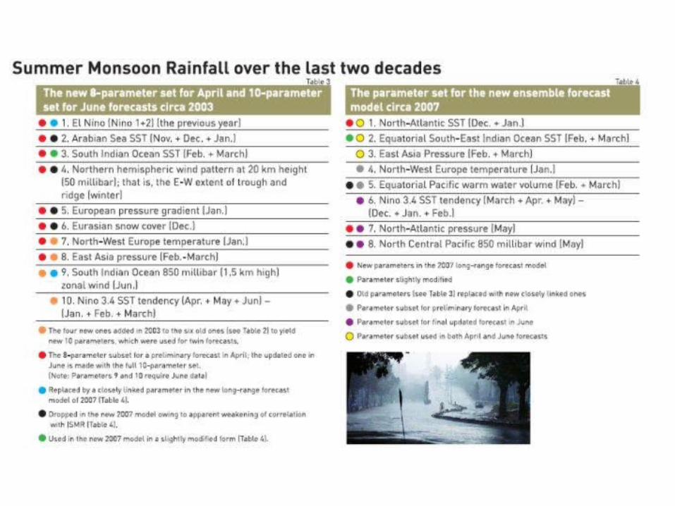
Predicting total monsoon rainfall (June-September)

• predicted by using its correlation with observed parameters

• The predictors keep changing with time • Several regression and neural network

based models are currently available• Indian Met. Dept (IMD) provides

statistical forecast in two stages, March/April May/June

No. Predictor (Period) Used for the forecasts in

1. North Atlantic Sea Surface Temperature (Dec. + Jan.)

April and June

2. Equatorial SE Indian Ocean Sea Surface Temp. (Feb. + March)

April and June

3. East Asia Mean Sea Level Pressure (Feb. + March)

April and June

4. NW Europe Land Surface Air Temperatures (Jan.)

April

No. Predictor (Period) Used for the forecasts in

5. Equatorial Pacific Warm Water Vol. (Feb.+March)

April

6. Central Pacific (Nino 3.4) Sea Surface Temperature Tendency (MAM-DJF)

June

7. North Atlantic Mean Sea Level Pressure (May)

June

8. North Central Pacific Wind at 1.5 Km above sea level (May)

June

Model

• IMD uses both linear and non-linear regression for their forecast

• use ensemble forecast large number of models are used for all possible

combinations of predictors only a few models with best skill are selected

• The forecast is the weighted average of the outcome of these models

• The model error 5% for April forecast 4% for June forecast

Short term Forecasting

• We have been interested in forecasting daily rainfall over a particular location a few days in advance.

• The government agency National Center for Medium Range Weather Forecasting (NCMRWF) provides daily forecasts, mainly to assist farmers.

Numerical Weather Prediction (NWP) Models

• Numerical Weather Prediction (NWP) models• Used to make short (1-3 days) and medium

(4-10) forecast• Navier Stokes equation is written on a

spherical grid covering the entire earth• use spherical polar coordinates • need to account for the earth’s rotation,

which makes it a non-inertial frame. This introduces fictitious Centrifugal and Coriolis force

• The variables are expanded in spherical harmonics, truncated up to a certain multipole, which determines the resolution of the grid.

• For example the current model is T254, which implies a grid size of 0.5ox0.5o

• 64 vertical levels

• 7.5 min time steps

Atmosphere

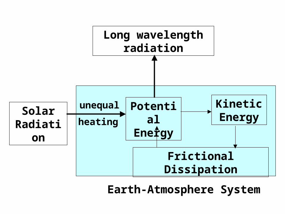
Earth-Atmosphere System

Potential Energy

Kinetic Energy

Frictional Dissipation

Solar Radiation

unequal

heating

Long wavelength radiation

General Circulation

• The inputs to the model are the initial conditions obtained by observations throughout the earth

temperature,

pressure,

wind velocity,

humidity etc

as a function of position and height

However the model is severely limited: The outcome, especially rainfall, is strongly

dependent on local factors This is particularly true in tropics where the

circulation is primarily driven by convection It is unfeasible to take all local factors into

consideration in a global model The prediction may change considerably by

very small changes in the input parameters

The output of the model is the desired prediction

The input data, especially high altitude balloon data, is severely limited

Also in many regions, especially India, the data quality is often not very good

There may also exist some unknown effects. An interesting possibility is effect of galactic cosmic rays

This possibility has been studied by Tripathi et al (CE, IITK)

Variation of low-altitude cloud cover, galactic cosmic rays and total solar irradiance (1984-1994). The cosmic ray intensity

data is from Huancayo observatory, Hawaii

Carslaw et al., 2002, Science

The physical links for the correlation is subject of research.

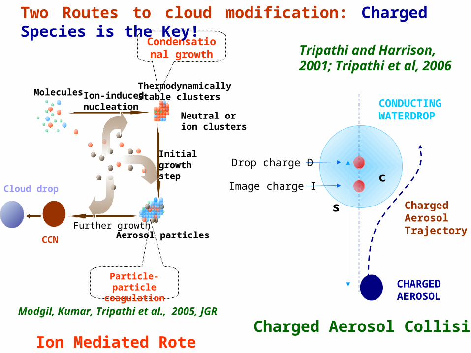
Ion Mediated Rote

Cloud drop

Further growth

CCN

Neutral or ion clusters

Molecules Ion-inducednucleation

ThermodynamicallyStable clusters

Initialgrowthstep

Aerosol particles

Condensational growth

Particle-particle coagulation

Tripathi and Harrison, 2001; Tripathi et al, 2006

s

Charged Aerosol Collision

Two Routes to cloud modification: Charged Species is the Key!

Drop charge D

Image charge I

CONDUCTINGWATERDROP

c

CHARGEDAEROSOL

ChargedAerosolTrajectory

Modgil, Kumar, Tripathi et al., 2005, JGR

Statistical Interpretation of NWF output

• It may be better to statistically correlate the model output with observations

• This is the technique used by NCMWRF to predict daily rainfall a few days in advance at a particular station

• The rainfall at a particular station is obtained by a rain gauge

• We have been trying to determine if neural network based relationship can improve the predictability.

Jain et al 1999, Jain and Jain 2002

Number Variable Level (hPa)

1-4 Geopotential 1000,850,700,500

5-8 Temperature 1000,850,700,500

9-12 Zonal wind comp. 1000,850,700,500

13-16 Meridional wind comp. 1000,850,700,500

17-20 Vertical velocity 1000,850,700,500

21-24 Relative humidity 1000,850,700,500

25 Saturation deficit 1000-500

26 Precipitable water 1000-500

27 MSLP

Number Variable Level (hPa)

28-29 Temperature gradient 850-700,700-500

30-31 Advection of TG 850-700,700-500

32-35 Advection of temp 1000,850,700,500

36-39 vorticity 1000,850,700,500

40-43 Advection of vorticity 1000,850,700,500

44-45 thickness 1000-500

45 Horizontal water vapor flux divergence

1000-500

46 Mean relative humidity 1000-500

47 Rate of change of moist static energy

1000-500

Scale invariance in daily rainfall

• The predictability of the quantity can often be judged by its distribution function.

• If the variable shows a normal distribution then large fluctuations from the mean value are improbable

• However a power law distribution

f(x) = x

implies no characteristic scale (scale invariant)

indicates an underlying chaotic behaviour

Distribution of daily rainfall: Kanpur

Fre

qu

enc

y

Precipitation (0.1mm)

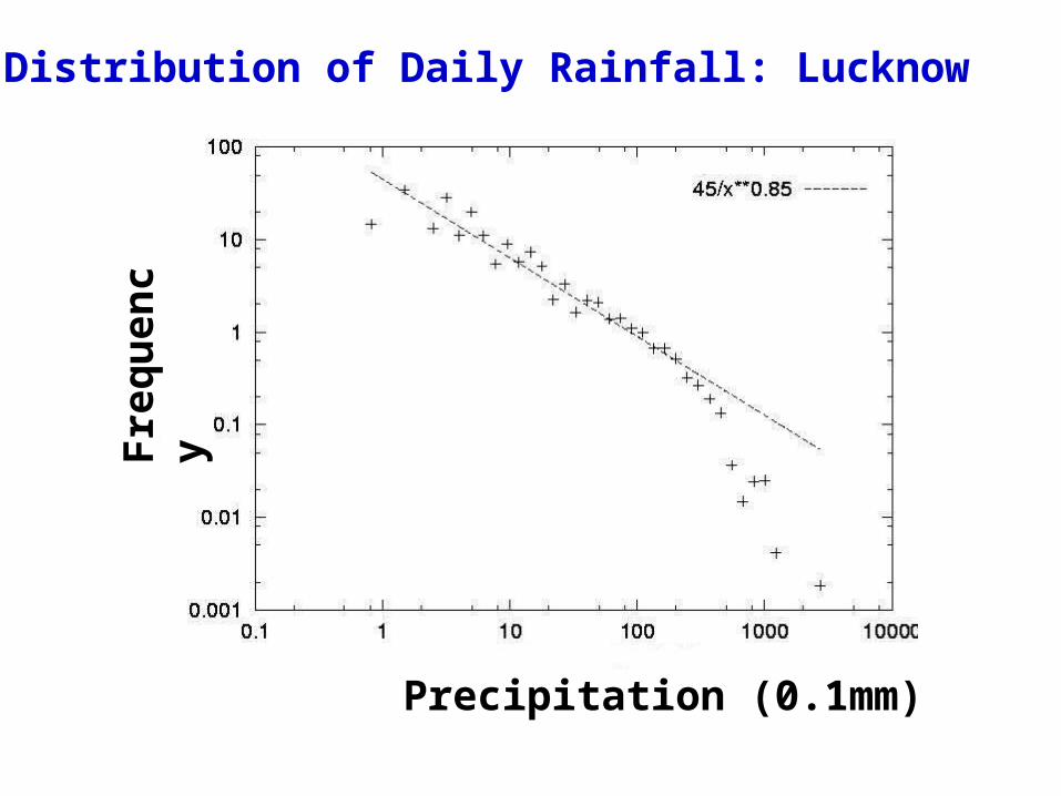
Distribution of Daily Rainfall: Lucknow

Fre

qu

enc

y

Precipitation (0.1mm)

SSM/I satellite data

A power law fits the distribution very well at low latitudes

Hourly rainfall Distribution

5S-10S

Rainfall rate in mm/hour

Fre

qu

enc

y

Hourly rainfall Distribution

15N-20N

Rainfall rate in mm/hour

Fre

qu

enc

y

Rainfall rate in mm/hour

Fre

qu

enc

y 0N-5N

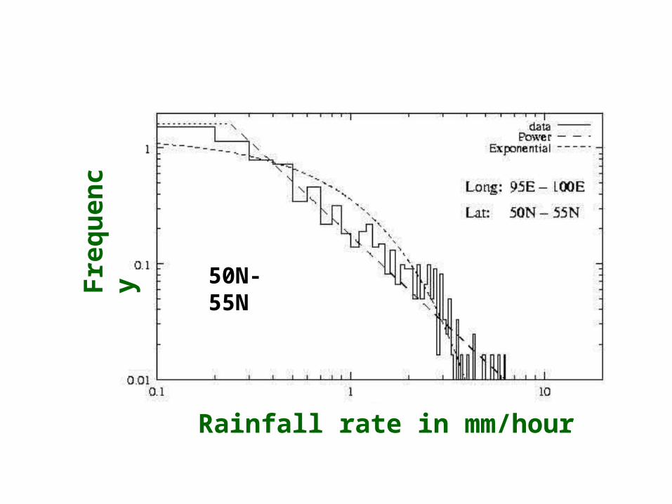
50N-55N

Rainfall rate in mm/hour

Fre

qu

enc

y

Rainfall rate in mm/hour

Fre

qu

enc

y

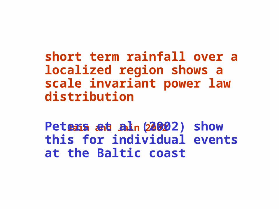
short term rainfall over a localized region shows a scale invariant power law distribution Jain and Jain 2002

Peters et al (2002) show this for individual events at the Baltic coast

Power law exponent as a function of the latitude f(x) = x

In tropics =1.130.14

At higher latitudes =1.3-1.6Jain and Jain, 2002

Latitude

Exp

on

ent

• It is better to define variable which we may have a better chance of predicting.

• Rather then using a single rain gauge it may be more appropriate to use the rainfall averaged over many rain gauges.

• The NWF has a grid size of order 100x100 Km. Hence its predictions should be interpreted as the average over the grid rather than for a particular location.

Predicting Daily Rainfall

• We studied daily rainfall forecast one day in advance• The following stations were considered: Delhi, Pune, Hyderabad, Bangalore,Bhubaneshwar • The output variable (y) is the daily rainfall• 47 input variables (xi), each at 9 grid points

surrounding the station. select by quadratic fitting over the 9 grid locations • 6 years data (1994-1999) from June to September for

Pune, Hyderabad, Bangalore,Bhubaneshwar For Delhi we consider data from June to August

Neural Networks Neural networks differ from statistical regression

techniques since one does not try to fit the output. By fitting we mean minimization of the error

yi is the predicted variable and y’i the measured variable.

Instead one only tries to learn the behaviour of the predictor.

Sum runs over the training set2' )( i

ii yy

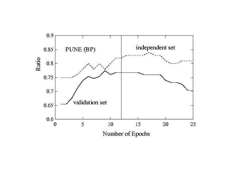
We terminate the training when the error in the validation becomes minimumThen the results are checked on an independent set.

While training one has to be careful that the network is not struck in some local minima

genetic algorithms or simulated anealing

Performance Indices

We shall predict (a) the probability of rainfall and (b) the actual rainfall (actually the cube

root of rainfall)

The skill of the model is tested by suitable performance indices

A model is skillful if it performs better than persistence model

Probability of Rainfall

Performance Indices:

Ratio = number correct / total

)]()()][()([

)()()()(..

wetMwetNdryMdryN

wetMdryMwetNdryNKH

N(dry) = no. of correctly predicted dry daysM(dry) = no. of incorrectly predicted dry days

2' )(1

.. ii

i yyN

SB

Amount of RainfallCube root of Precipitation

Performance Index: Root Mean Square Error

2' )(1

ii

i yyN

RMSE

Results (Pune)

Model Network Training

error

B.S. Ratio H.K.

LR 41.81 0.164 0.769 0.485

NN

CG

42-3-1-1 42.3 0.154 0.806 0.584

NN

BP

42-4-3-1 43.0 0.151 0.785 0.532

Results (Hyderabad)

Model Network Training

error

B.S. Ratio H.K.

LR 56.9 0.233 0.620 0.195

NN

CG

42-4-4-1 50.8 0.227 0.694 0.360

NN

BP

42-3-1 57.5 0.217 0.661 0.277

Results (Bangalore)

Model Network Training

error

B.S. Ratio H.K.

LR 62.88 0.228 0.636 0.176

NN

CG

42-4-4-1 53.2 0.225 0.678 0.318

NN

BP

42-4-4-1 62.2 0.230 0.686 0.332

Results (Bhubaneshwar)

Model Network Training

error

B.S. Ratio H.K.

LR 53.9 0.219 0.644 0.240

NN

CG

42-4-4-1 54.4 0.211 0.652 0.332

NN

BP

42-4-4-1 53.8 0.209 0.669 0.344

Results (Delhi)

Model Network Training

error

B.S. Ratio H.K.

LR 36.9 0.191 0.723 0.377

NN

CG

42-1 35.2 0.198 0.723 0.382

NN

BP

42-1 42.2 0.167 0.750 0.436

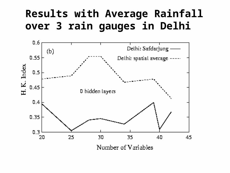
Results with Average Rainfall over 3 rain gauges in Delhi

Results with Average Rainfall over 3 rain gauges in Delhi

Results with Average Rainfall over 3 rain gauges in Delhi

Results with Average Rainfall over 3 rain gauges in Delhi

Conclusions

• We find that in tropics the short term rainfall distribution follows a universal power law with exponent 1.130.14

• Predicting daily rainfall at a particular rain gauge appears to be difficult

• Neural Networks give a modest improvement over linear regression results

• We recommend that instead of a single rain gauge one should use a spatial average over many rain gauges, which gives significantly better results

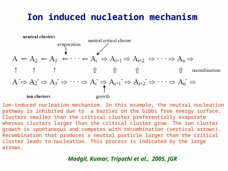
Ion induced nucleation mechanism

Ion-induced nucleation mechanism. In this example, the neutral nucleation pathway is inhibited due to a barrier on the Gibbs free energy surface. Clusters smaller than the critical cluster preferentially evaporate whereas clusters larger than the critical cluster grow. The ion cluster growth is spontaneous and competes with recombination (vertical arrows). Recombination that produces a neutral particle larger than the critical cluster leads to nucleation. This process is indicated by the large arrows.

Modgil, Kumar, Tripathi et al., 2005, JGR

Freezing probability from electrical Enhancement of aerosol collection rate P, calculated as a function of particle elementry charges J. Neutral (supercooled) droplets of radii 52, 40, 32, 26 and 18 µ m are considered to collect aerosol particles of radii 0.4, 0.4, 0.5, 0.6and 0.4 µ m Respectively.

Tripathi and Harrison, , 2002

plotted as a function of ion asymmetry factor x for various aerosol radii a.N20 and N-20 are number concentrationsof aerosols carrying -20 and +20 charges respectively and Z(103 cm-3 )is the total number concentration. Horizontal line indicates the regionabove which 1 particle per cm will be present.(b) Same as (a) except for

N10 and N-10 .

20 20N N

Z

More ice formation through contact ice nucleation in cold clouds