monotone difference approximations for scalar conservation ... · monotone difference...
TRANSCRIPT
MATHEMATICS OF COMPUTATION, VOLUME 34, NUMBER 149
JANUARY 1980, PAGES 1-21
Monotone Difference Approximations
for Scalar Conservation Laws
By Michael G. Crandall and Andrew Majda*
Abstract. A complete self-contained treatment of the stability and convergence proper-
ties of conservation-form, monotone difference approximations to scalar conservation
laws in several space variables is developed. In particular, the authors prove that gener-
al monotone difference schemes always converge and that they converge to the physical
weak solution satisfying the entropy condition. Rigorous convergence results follow
for dimensional splitting algorithms when each step is approximated by a monotone
difference scheme.
The results are general enough to include, for instance, Godunov's scheme, the
upwind scheme (differenced through stagnation points), and the Lax-Friedrichs scheme
together with appropriate multi-dimensional generalizations.
Introduction. Perhaps the simplest mathematical models exhibiting behavior typ-
ical of that encountered in inviscid continuum mechanics are the initial-value problems
for a scalar conservation law. These problems are of the form
( N\ (0 «f + L fiWxi = 0, fort>0,x = (xx,...,xN)GRN,
(0.1) '=i
( (ii) u(x, 0) = u0(x), for x 6 R^,
where the f¡ are smooth real-valued functions and u is a scalar. It is well known (see
[14]) that even if the initial value «0 is smooth, the solution to (0.1) typically develops
discontinuities as t increases to some t0 > 0 (i.e. shock waves form). Thus the differen-
tial equation must be understood in a generalized or weak sense. However, there can
be an infinite number of generalized solutions of (0.1) with the same initial data u0;
and an additional principle, the entropy condition, is needed to select the unique
"physical" weak solution (see [14]).
The main new result of this work establishes the convergence of general conserva-
tion-form, monotone difference approximations to (0.1) to the unique generalized solu-
tion which satisfies the entropy condition. For notational simplicity in the sequel we
restrict the presentation to the case N = 2 for the most part. The corresponding defi-
nitions and results for the general case will be clear from this. For N = 2
we write (x, y) rather than (xx, x2). Selecting mesh sizes Ax, Ay, At > 0, the value
Received February 12, 1979.
AMS iMOS) subject classifications (1970). Primary 65M10, 65M05.
Key words and phrases. Conservation laws, shock waves difference approximations, entropy
conditions.
•Partially supported by Sloan Foundation Fellowship. Sponsored by the United States Army
under Contract No. DAAG29-75-C-0024.
© 1980 American Mathematical Society
0025-5718/80/0000-0001/$06.25
1
License or copyright restrictions may apply to redistribution; see https://www.ams.org/journal-terms-of-use
2 MICHAEL G. CRANDALL AND ANDREW MAJDA
of our numerical approximation at iJAx, kAy, nAt) will be denoted by £/"fc. Capital
letters U, V, etc. will denote functions on the x, y lattice A = {(jAx, kAy) :j, k are
integers}; and the value of U at (jAx, kAy) will be written U¡k. Thus U", the state
of our numerical approximation at the level nAt, is a function on A with values £/"fc.
The standard notations \x = At/Ax, \y = At/Ay, (A* U)jk = Uj+ x >k - U¡ k,
(Ay+ U)jk = Uj k+ j - Uj k, etc., will be used. The difference approximations of (0.1)
of interest here are explicit marching schemes of the form
(0.2) u¡xx = Giir¡_p<k_r,..., Uf+q+UkT,+i),
where p, s, q, r are nonnegative integers and G is a function of (p + q + 2)(r + s + 2)
real variables. (We are ignoring X*, X^ dependence for the moment, as these quantities
will typically be fixed.) To simplify notation, (0.2) will be written as
(0.3) U" + l =GiU"),
with the choice of p, s, q, r dictated by the context. The difference approximation
(0.2)-(0.3) is said to have conservation form (see [10]) if there are functions g,, g2
such that
GiU),;k = GiUhPik_r,...,Ui+q + Xtk+s+x)
(°-4) = UUk - \xA\gxiUhp¡k_r, ..., Ui+q>k+s+x)
-VAlg2iUhp^r,...,Uj+q + Xtk+s).
In order that (0.3) be consistent with (0.1) when (0.4) holds we must have
(0.5) g.(u,_u) = f¡(u) for u G R and i = 1, 2.
The functions g¡ are called the numerical fluxes of the approximation.
Finally, the difference approximation is monotone on the interval [a, b] if
G(ax, . . . , û(p+q + 2)(i-+s+2))1S a nondecreasing function of each argument a¡ so
long as all arguments lie in [a, b].
It follows from the results of [13] that for uQ G L°°(R2) n Z,'(R2) there is a
unique weak solution u G Z,°°(R2 x [0, °°)), which satisfies the entropy condition of
[13]. (See Section 2 for more details.) Moreover, we can write u(x, y, t) = (5(f)u0) •
(x, y), where S(t) :Ll(R2) D Z~(R2) -> Z,!(R2) n ¿°°(R2) for each t > 0 and t —►
S(t)uQ is continuous into /^(R2)- To compute this solution numerically we set
(°-6) Ul=^LUkuo^y)^dy,
where
Rj,k - [(/ - H)**. if + ^)Ax) x [(k - V4)Ay, (* + W)áy),
and define Un+X from U" by (0.3). Finally, put x?fc = characteristic function of /? fc
x [«Ar, in + l)At) and
(O?) «**=± t U»A.n = 0 ;,Ar=-o°
License or copyright restrictions may apply to redistribution; see https://www.ams.org/journal-terms-of-use
DIFFERENCE APPROXIMATIONS FOR SCALAR CONSERVATION LAWS 3
The main result is
Theorem 1. Suppose u0 GLX(R2) n L°°(R2) anda < u0 < b a.e. Let (0.2)
be a consistent conservation-form difference approximation to (0.1X0 which is mono-
tone on [a, b] and which has Lipschitz continuous numerical fluxes g¡, i = 1,2. Let
uAt be given by (0.2), (0.6), (0.7). Then as At —► 0 with Xx, X*" fixed, uAt converges
to S(t)u0 in LX(R2) uniformly for bounded t>0. More precisely,
(0.8) Km sup ff luAt(x,y,t)-S(t)uo(x,y)\dxdy = 0Af-i-0 0<f<r R
for each T>0.
Reviewing the definitions, (0.8) can also be restated as
Î0 9Ï AUm SUP ZiR.^U/,kS(t)uo(x,y)\dxdy = 0.\y-y) Af->o o<t<T ¡,k i.k
nAt<t<in+l)At
It should be recalled that even if N = 1 and fx is convex, nonmonotone schemes such
as the Lax-Wendroff scheme can converge to solutions which violate the entropy con-
dition; see [10] and [18]. The result of Theorem 1 applies to the popular dimensional
splitting algorithms; see [8], [17], [21]. This follows from simple observations. For
example, consider the one-dimensional conservation laws
(o.io) i(i) «v + 'iO*,.-*j(ii) wt+f2(w)y = 0.
If
(o.io j© y?+l=Gx(vf_p,...,r}+q+x),
(ii) W"k + x=G2(W"k_„...,W"k+s+x),
are conservation-form difference approximations of (0.10)(i), (ii), respectively, Lax has
observed that the scheme defined by
(0.12) | i-k ^l^Ui-p,k ' • • • ' Uj+q+l,kh
[ U?,m ~ G2Í^l,m-r' • • -» tf.m +s+ l)'
has conservation form and is consistent with (0.1); see [2] or check the definitions.
When Gx and G2 are also monotone on [a, b] the scheme in (0.12) will be monotone
on [a, b]. (Since a < K+;<Z> for-p <Kq + 1 implies a < Gx(V¡_p,..., V¡+q + x)
< b by Proposition 3.1(b) below, this is evident.) Thus, Theorem 1 applies to the split
scheme (0.12). This fact, along with other results concerning splitting algorithms is
developed in [17].
The plan of this work is as follows: In Section 1 various monotone difference
schemes to which Theorem 1 applies are recalled. These include the Lax-Friedrichs
scheme, the upwind scheme (differenced through stagnation points) and Godunov's
scheme. The construction of a wide variety of multi-dimensional schemes from the
License or copyright restrictions may apply to redistribution; see https://www.ams.org/journal-terms-of-use
4 MICHAEL G. CRANDALL AND ANDREW MAJDA
above one-dimensional ones is discussed. In view of these examples, many of the re-
sults of Le Roux [16] for specific schemes in a single space dimension are included
in our general approach. Section 2 is a review of some basic facts about solutions to
(0.1) and some function spaces and estimates needed in the proof of Theorem 1. We
discuss the stability of monotone conservation-form difference schemes in Section 3.
In particular, we prove that such schemes define Lx contractions; this was proved by
Jennings [11] in the case of one space variable, but even there our proof, based on
a lemma of Crandall and Tartar [5], is simpler. In Section 4 we verify that if solutions
of monotone conservation-form difference approximations converge, the limit satisfies
the entropy conditions. This was proved by Harten, Hyman and Lax in [10] for N =
1 ; however, we build a different discrete entropy flux which yields a simpler proof for
general N and requires only continuity of the numerical fluxes. This generality is use-
ful for applications. (See Section 1 and [16].) The various results of Sections 2, 3, 4
are pieced together to prove Theorem 1 in Section 5. In Section 6 we briefly discuss
the inhomogeneous equation.
In fact, our arguments yield more than Theorem 1 states, for the existence of
the solution S(t)u0 of (0.1) is established while proving convergence (see Section 5).
See Conway and Smoller [3], Doughs [6], and Kojima [12] for earlier uses of the
(monotone) Lax-Friedrichs difference approximation to prove existence. Oharu and
Takahashi prove this scheme converges to the solution satisfying the entropy condition
via nonlinear semigroup methods in [19].
Added in Proof. Kuznecov and Volosin [23], a paper we uncovered on the
day it was necessary to return the corrected proofs, states the main result of this work
together with an error estimate under stronger regularity assumptions than used here.
1. Examples. In this section we present a variety of difference schemes to
which Theorem 1 applies. Later sections are independent of the current one.
We begin with several well-known schemes in the case A^ = 1. So long as A^ = 1
we will write /, g in place of fx, gx. For a single-space variable the Lax-Friedrichs
scheme is given by
(l.i) «;+1 = w¡ -~Ax0f(ui) + \ Aiààq.
Equivalen tly,
uJ + x=uJ-XxAx+g(u¡,ui_x),
where the numerical flux g is given by
f(U:) + f(uhx) JgiUf, Uj_x) =-— («, - Uhl).
The conservation form and consistency are obvious. A simple analysis reveals that
(1.1) is also monotone on [a, b] provided that the C.F.L. condition
(1.2) X* max l/'(«) I < 1a<u<b
License or copyright restrictions may apply to redistribution; see https://www.ams.org/journal-terms-of-use
DIFFERENCE APPROXIMATIONS FOR SCALAR CONSERVATION LAWS 5
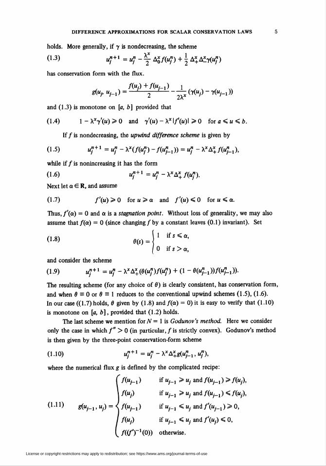
holds. More generally, if y is nondecreasing, the scheme
0-3) WJ+X = «; - y Axfiuf) + I A* Al7(w")
has conservation form with the flux.
/(«,)+/("/-!) 1giu,, uhx) =-— (T(M/.) - yiUj_x))
and (1.3) is monotone on [a, b] provided that
(1.4) 1 - Xxy'iu) >0 and T'(w) - X*l/'(«)l > 0 for a < u < b.
If / is nondecreasing, the upwind difference scheme is given by
(1.5) u;+1 = «; - x*(/(Wp -/(«;_,)) = «; - x*a*/o^l,),
while if/is nonincreasing it has the form
(1.6) «;+1 =u;"- XxAx+ /(«?).
Next let a G R and assume
(1.7) f\u) >0 foru>a and /'(«) < 0 for u < a.
Thus, /'(a) = 0 and a is a stagnation point. Without loss of generality, we may also
assume that/(a) = 0 (since changing/by a constant leaves (0.1) invariant). Set
H in 1 if s < a,Í1-8) fl(s) =
(0 ifs>a,
and consider the scheme
(i.9) «;+>. «; - x*a* (ö(«;)/(«7) + o - «(«?_!))/(«"-i))-
The resulting scheme (for any choice of 6) is clearly consistent, has conservation form,
and when 6 = 0 or ô = 1 reduces to the conventional upwind schemes (1.5), (1.6).
In our case ((1.7) holds, 6 given by (1.8) and /(a) = 0) it is easy to verify that (1.10)
is monotone on [a, b], provided that (1.2) holds.
The last scheme we mention for N = 1 is Godunov's method. Here we consider
only the case in which /" > 0 (in particular,/is strictly convex). Godunov's method
is then given by the three-point conservation-form scheme
(1 -10) u1 + x = «; - XxAx+giu?_x, ul),
where the numerical flux g is defined by the complicated recipe:
/(«,-_,) if uj_x > Uj and f(uM) > /(«,),
fiUj) if uf_x > uf and fiu¡_x ) < fiu¡),
Í1 -10 stuM, Uj) = <¡ fiUj_x ) if Uj_x < Uj and /*(«,_, )>0,
fiUj) if «/._1 < Uj and /'(uy) < 0,
fi(f'Tx(0)) otherwise.
License or copyright restrictions may apply to redistribution; see https://www.ams.org/journal-terms-of-use
6 MICHAEL G. CRANDALL AND ANDREW MAJDA
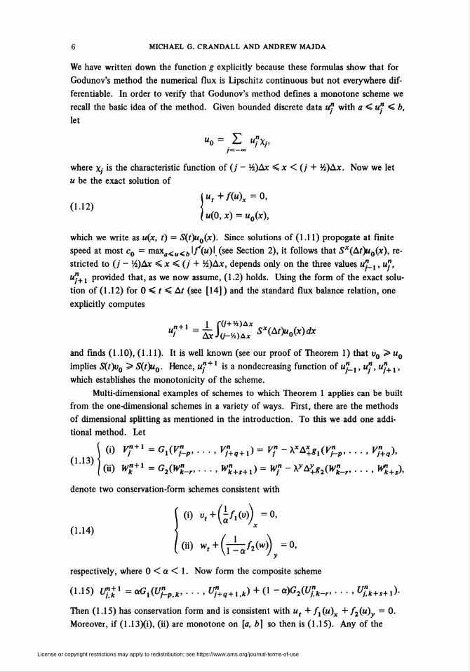
We have written down the function g explicitly because these formulas show that for
Godunov's method the numerical flux is Lipschitz continuous but not everywhere dif-
ferentiable. In order to verify that Godunov's method defines a monotone scheme we
recall the basic idea of the method. Given bounded discrete data m" with a < u" < b,
let
«o = £ ufxj,/=-
where x¡ is the characteristic function of (/' - Yi.)Ax < x < if + ft)Ax. Now we let
u be the exact solution of
í « + fiu)x = 0,(1.12)
/ w(0, x) = u0ix),
which we write as u(x, t) = Sit)uQix). Since solutions of (1.11) propogate at finite
speed at most c0 = maxa<u<2)l/'(u)l (see Section 2), it follows that 5x(Ar)w0(x), re-
stricted to (/ - *A)Ax < x < (/ + V>)Ax, depends only on the three values m"_j , u?,
Uy+1 provided that, as we now assume, (1.2) holds. Using the form of the exact solu-
tion of (1.12) for 0 < t < Ar (see [14]) and the standard flux balance relation, one
explicitly computes
„4-1 1 f(/+%)Ax<I=ÍW, SxiAt)u0ix)dx
and finds (1.10), (1.11). It is well known (see our proof of Theorem 1) that v0 > u0
implies Sit)v0 > S(r)w0. Hence, u"+ x is a nondecreasing function of u"_x, u", u"+ x,
which establishes the monotonicity of the scheme.
Multi-dimensional examples of schemes to which Theorem 1 applies can be built
from the one-dimensional schemes in a variety of ways. First, there are the methods
of dimensional splitting as mentioned in the introduction. To this we add one addi-
tional method. Let
| (i) V?+x = GxiVf_p, ..., V?+q+x) =Vf- XxAx+gxiV¡Lp, ..., Vf+q),
(U3) j (Ü) W"k + X = G2iW"k_„ ..., W"k+S+X) = Wf - XyAy+g2iW"k_r, ..., W"k+sl
denote two conservation-form schemes consistent with
(1.14)
(o »f+(s/i(«o) =0'
(ii) wf + (j^/2(vvj) -0,
respectively, where 0 < a < 1. Now form the composite scheme
(1.15) VfP = aGxiU¡LPik, ..., Vf+q+uk) + (1 -<*)G2iUZk_r, ..., U£k+S+X).
Then (1.15) has conservation form and is consistent with ut + fxiu)x + f2iu)y = 0.
Moreover, if (1.13)(i), (ii) are monotone on [a, b] so then is (1.15). Any of the
License or copyright restrictions may apply to redistribution; see https://www.ams.org/journal-terms-of-use
DIFFERENCE APPROXIMATIONS FOR SCALAR CONSERVATION LAWS 7
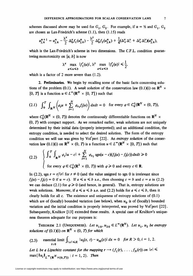
schemes discussed above may be used for Gx, G2. For example, if a = xk and Gx, G2
are chosen as Lax-Friedrich's scheme (1.1), then (1.15) reads
«Ei1 = «/% - y KflHtc) - f Ao/2Kk) + fc%& + AlAiyul,),
which is the Lax-Friedrich's scheme in two dimensions. The C.F.L. condition guaran-
teeing monotonicity on [a, b] is now
Xx max \f'xiu)\,Xy max I/2(m)I<-,a<u<b a<u<b
which is a factor of 2 more severe than (1.2).
2. Preliminaries. We begin by recalling some of the basic facts concerning solu-
tions of the problem (0.1). A weak solution of the conservation law (0.1)(i) on RN x
[0, T] is a function u G L°°iRN x [0, T]) such that
(2.1) JQr f n Lu + £ <fix/fi*)j dxdt = 0 for every y G C\(RN x (0, T)),
where Cq(Rn x (0, 7)) denotes the continuously differentiable functions on R^ x
(0, T) with compact support. As we remarked earlier, weak solutions are not uniquely
determined by their initial data (properly interpreted); and an additional condition, the
entropy condition, is needed to select the desired solution. The form of the entropy
condition we will use was given by Vol'pert [22]. An entropy solution of the conser-
vation law (0.1X0 on R^ x (0, T) is a function u GL°°(RN x [0, T]) such that
i io J*Riv *> "cl + ? **t s^u "cm»)-m)d**>0
for every <p G CX(R2 x (0, T)) with <p > 0 and every c G R.
In (2.2), sgn r = r/lrl for r =£ 0 (and the value assigned to sgn 0 is irrelevant since
//(") ~ fiic) = 0 if u = c). If a < u < ¿> a.e., then choosing c = ft and c = a in (2.2)
we can deduce (2.1) for i/> > 0 (and hence, in general). That is, entropy solutions are
weak solutions. Moreover, if a < u < ft a.e. and (2.2) holds for a < c < Z», then it
clearly holds for all c. The existence and uniqueness of entropy solutions of (0.1)
which are of (locally) bounded variation (see below), when uQ is of (locally) bounded
variation and the initial condition is properly interpreted, was proved by Vol'pert [22].
Subsequently, Kruzkov [13] extended these results. A special case of Kruzkov's unique-
ness theorem adequate for our purposes is:
Theorem 2.1 (Uniqueness). Let ux0, u20 EL°°iRN). Let ux,u2 be entropy
solutions of (0.1)(i) on RN x (0, T) for which
(2.3) essential limit J, , <Ä I",-(*. 0 ~ "i0(*)' dx = 0 for R> 0, i = 1,2.no x
Let L be a Lipschitz constant for the mapping r —► (/i(>"), • • • »/v(r)) on 'rl ^
IMX{|"<li-(R^x(o,r)):fasl'2}- Then
License or copyright restrictions may apply to redistribution; see https://www.ams.org/journal-terms-of-use
8 MICHAEL G. CRANDALL AND ANDREW MAJDA
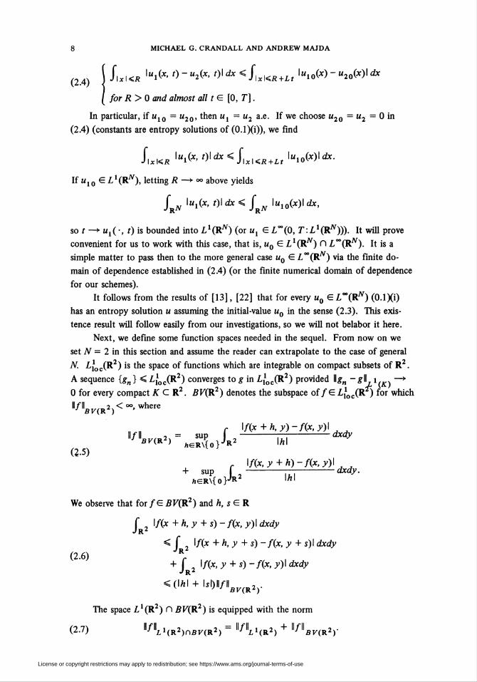
i L\<r iuib>V-»2(x.t)\dx<f{xKR+Lt\u1Qix)-u2Q<x)\dx
forR>0 and almost all t G [0, T].
In particular, if uxo = u20, then ux = u2 a.e. If we choose u20 = u2 = 0 in
(2.4) (constants are entropy solutions of (0.1)(i)), we find
SfxKR \»iix-t)\dx<hx¡<R+Lt\uxoix)\dx.
If u10 G LxiRN), letting # —► °° above yields
f \uxix, t)\ dx < f \uxoix)\dx,K R
so r -> «,(-, 0 is bounded into LX(RN) (or u, G L~(0, T:Ll(RN))). It will prove
convenient for us to work with this case, that is, u0 G LxiRN) fi L°°iRN). It is a
simple matter to pass then to the more general case u0 G ¿"(R^) via the finite do-
main of dependence established in (2.4) (or the finite numerical domain of dependence
for our schemes).
It follows from the results of [13], [22] that for every u0 G L°°iRN) (0.1X0
has an entropy solution u assuming the initial-value uQ in the sense (2.3). This exis-
tence result will follow easily from our investigations, so we will not belabor it here.
Next, we define some function spaces needed in the sequel. From now on we
set N = 2 in this section and assume the reader can extrapolate to the case of general
N. L\oc(yt}) is the space of functions which are integrable on compact subsets of R2.
A sequence {gn } < L¡oc(R2) converges to g in Lloc(R2) provided \\gn - g\\ i —*■
0 for every compact K CR2. BV(R2) denotes the subspace of /G L¡oc(R ) for which
ll/lW(R2)<00'where
(2.5)
f ^ix+h,y)-f(x,y)\ j jW*vf*^= sup J 2-¡ül-dxdy
+ sup f7,eR\{o}JRi
\f(x,y + h)-f(x,y)\
\h\dxdy.
(2.6)
We observe that for /G BV(R2) and h, s G R
T \f(x+h,y + s)-f(x,y)\dxdyJR2
( , \f(x + h,y + s)- f(x, y + s)\ dxdy
f \fix,y + s)-fix,y)\dxdyJr2
<(IAI + lsl)ll/ll ,.v ' J BViR2)
The space Z,!(R2) O 7ÍK(R2) is equipped with the norm
(2.7) ll^llLi(R2)nñnR2) = lflLH*2) + mBViR2Y
+
License or copyright restrictions may apply to redistribution; see https://www.ams.org/journal-terms-of-use
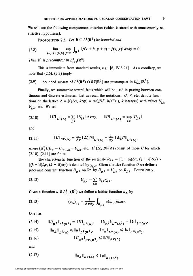
DIFFERENCE APPROXIMATIONS FOR SCALAR CONSERVATION LAWS 9
We will use the following compactness criterion (which is stated with unnecessarily re-
strictive hypotheses).
Proposition 2.2. Let H C Lx (R2 ) be bounded and
(2.8) lim sup | \fix + h,y + s) - fix, y)\ dxdy = 0.ih,s)->iO,0) fEH jR
Then H is precompact in L¡oc(R2).
This is immediate from standard results, e.g., [6, IV.8.21]. As a corollary, we
note that (2.6), (2.7) imply
(2.9) bounded subsets of LxiR2) n BV(R2) are precompact in L¡oc(R2).
Finally, we summarize several facts which will be used in passing between con-
tinuous and discrete estimates. Let us recall the notations. U, V, etc. denote func-
tions on the lattice A = {(/Ax, kAy) = Atij/Xx, b/Xy):j, k integers} with values f/- k,
Vjk, etc. We set
(2.10) llf/llLi(A)=Z \Uiik\AxAy, lJ7i - sup \U/>k\j,k j,k
and
(2.11) '^(4) = ¿l^(/lLl(A) + l IA^I£l(Ä),
where (A+(7)/jfc = Uj+Xk - Ujk, etc. LX(A), BV(A) consist of those Ufor which
(2.10), (2.11) are finite.
The characteristic function of the rectangle R • k = [(j - M)Ax, (j + ]6.)Ax) x
[(k - lA)Ay, (k + *A)Ay) is denoted by x,- k- Given a lattice function U we define a
piecewise constant function (7r2 on R2 by ¿7r2 = Ujk on Rj k. Equivalently,
(2-12) UR2=ZVj,kXj,k.i.k
Given a function u G ¿11oc(R2) we define a lattice function «A by
(213) M*"^^*')**-
One has
(2-14) lt/RlliI(Rl) = lli/llLl(A), I£Ar2Il.(r2) = IWL.(A),
(2.15) H«AllLi(A) < l«lLi(Ba). I«AIL-(A) < ■«■L-(Ba).
(2.16) IICW(R2)<IIC/lW)>
and
(2-1?) ll"A«BK(A)<««»SF(R2)-
License or copyright restrictions may apply to redistribution; see https://www.ams.org/journal-terms-of-use
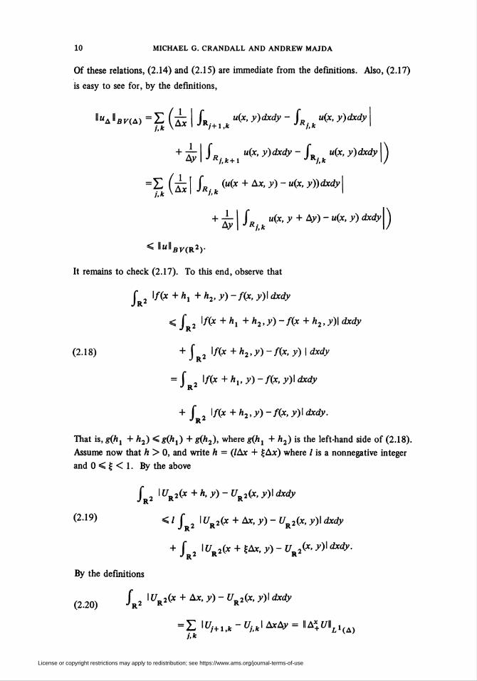
10 MICHAEL G. CRANDALL AND ANDREW MAJDA
Of these relations, (2.14) and (2.15) are immediate from the definitions. Also, (2.17)
is easy to see for, by the definitions,
""a W) = £ (¿ | Jr/+1 k u(-x' y>)dxdy - Sr, k "(*> y)dxdy
+ ÂÏÏ J p "(*' >')dxi^ - JR "(*, y)dxdy )Ay I J Rj,k+1 JKj,k /
=L ( Äv I L. ("(* + AX' ^ ~ "(*' ̂̂ ^I
+ Ay■j- I f u(pc, y + Ay) - uix, y) dxdy )Ay I J Kj,k /
< llwllSF(R2).
It remains to check (2.17). To this end, observe that
f 2 \fix+hx + h2,y)-fix, y)l dxdyJ R
< Jr2 l/C« + hx + /i2, >>) - fix + h2, y)\ dxdy
(2.18) + \ 2\fix+h2,y)- fix, y) | dxdy
= f , \fix+hx,y)-fix, y)\ dxdy
+ r, i/ix+zi,^)-/^^!^^.JR2
That is, ̂ (/ij + h2) < s^) + #(/i2), where gQix + h2) is the left-hand side of (2.18).
Assume now that h > 0, and write h = (/Ax + £Ax) where / is a nonnegative integer
and 0 < £ < 1. By the above
/R2 ' ^R2^ + h' y) " ^R2^' *>' dxdy
(2-19) </{r2I í/r2(* + Ax, y) - í/r2(x, y)l dxdy
+ f 2 I tfR2(* + ?Ax, y) - ?7r2(*> JO' <^-
By the definitions
(2.20) SR2 ' M* + A*' *> - M* '>' d^
= Z\Uj+i,k-Ujik\AxAy=\\Ax+U\\LHA)j,k
License or copyright restrictions may apply to redistribution; see https://www.ams.org/journal-terms-of-use
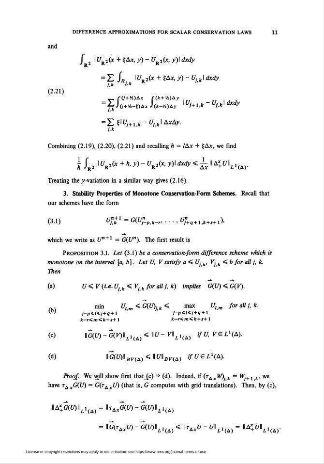
DIFFERENCE APPROXIMATIONS FOR SCALAR CONSERVATION LAWS 11
and
/ 2 I UR2Íx + £Ax, y) - <7r2(x, y)\ dxdy
(2.21)
= Z Sr. iuR2Í* + %*x, y) - Uf¡kI dxdyj, k t,k
Çij+Y>)Ax Çik+V>)Ay .
= HÜUj+i,k-Ujik\AxAy.j,k
Combining (2.19), (2.20), (2.21) and recalling h = lAx + £Ax, we find
\ Jr2 I U%2ix + h,y)- UR2ix, y)\ dxdy < ¿ Il A^II¿1(A).
Treating the j>-variation in a similar way gives (2.16).
3. Stability Properties of Monotone Conservation-Form Schemes. Recall that
our schemes have the form
(3.1) U"k 1 = GiU"-p,k-r' • • • ' U"+q+l,k + s+l)<
which we write as U" + x = GiU"). The first result is
Proposition 3.1. Let (3.1) be a conservation-form difference scheme which is
monotone on the interval [a, b]. Let U, V satisfy a < £/• k, V- k < b for all j, k.
Then
(a) U < V (i.e. Ujk < Vjk for all j, k) implies GiU) < G(F).
(b)
(c) WGÍU)-GÍV)\\lHa)<\\U-V\\lHa) ifU,VGLxiA).
(d) llG(í/)llBnA)<llt/IW(A) ifUGLx(A).
Proof. We will show first that_{c) •» (d). Indeed, if ÍTAxW)¡k = W¡+, ;fc, we
have TAxGiU) = GítAxLÍ) (that is, G computes with grid translations). Then, by (c),
11 K<kWLi (A) = llrAx«J(LO-G(LOIILl(A)
= \\G(tAxU)-G(U)\\lX(a)<\\tAxU-U\\lX{a)=\\Ax+U\\lX(a).
min Ulm < GiU)jk < max Ulm for all j, k.j-p<Kj+q+l j-p^Kj+q+l
k-r<m<k + s+l k-r<m<k + s+l
License or copyright restrictions may apply to redistribution; see https://www.ams.org/journal-terms-of-use
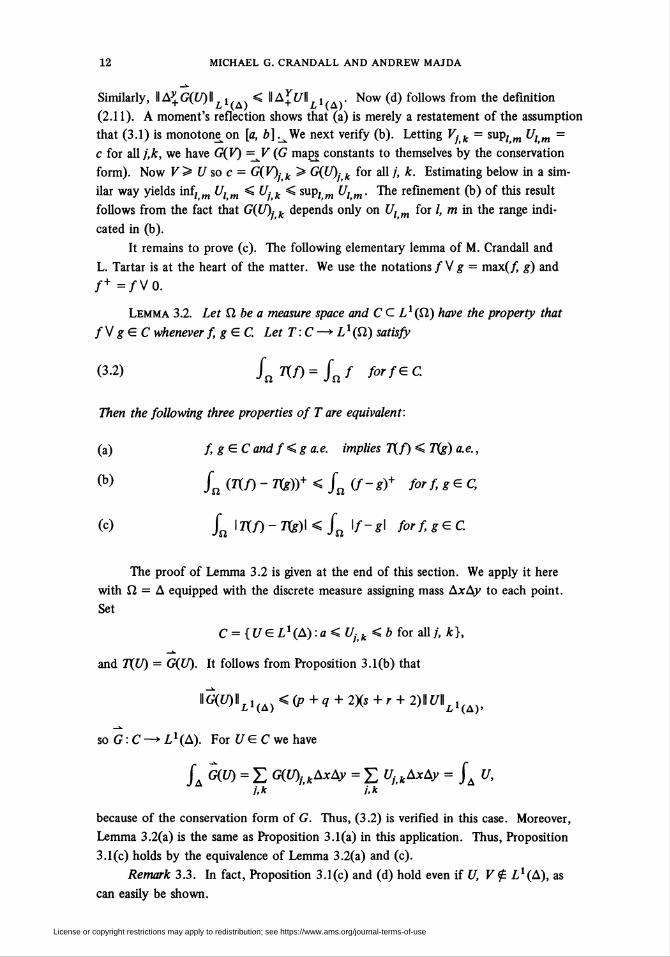
12 MICHAEL G. CRANDALL AND ANDREW MAIDA
Similarly, IIA*GiU)IIL, < ^^+u^Li(Ay Now (d) f°U°ws from the definition
(2.11). A moment's reflection shows that (a) is merely a restatement of the assumption
that (3.1) is monotone^ on [a, ¿>]^We next verify (b). Letting V¡ k = sup/m Ulm =
c for all j,k, we have GiV) =V (G maps constants to themselves by the conservation
form). Now V > U so c = C7(F). k ~> G(U)j k for all /, k. Estimating below in a sim-
ilar way yields inf, m U¡ m < Ujk < sup/m Ulm. The refinement (b) of this result
follows from the fact that G(U)j k depends only on Ulm for l, m in the range indi-
cated in (b).
It remains to prove (c). The following elementary lemma of M. Crandall and
L. Tartar is at the heart of the matter. We use the notations / V g = max(/, g) and
/+ =/V0.
Lemma 3.2. Let £1 be a measure space and C C Lx(Í2) have the property that
/ V gGC whenever fig EC. Let T : C -+ Lx (£2) satisfy
(3.2) SQnn = iaf for fee
Then the following three properties of T are equivalent:
(a) fg<ECandf<g a.e. implies Tif) < Tig) a.e.,
(b) Sa(.Tif)-T(g))+<faif-g)+ for fi geC,
(c) ¿lîl/)- T(g)\ <fa\f-g\ for figeC.
The proof of Lemma 3.2 is given at the end of this section. We apply it here
with £2 = A equipped with the discrete measure assigning mass AxA^ to each point.
Set
C = { U G I,1 (A) : a < Ujk < b for all /, *},
and TiU) = GiU). It follows from Proposition 3.1(b) that
l^hxiA) <iP+<l + 2)(s+r + 2)11 U\\L 1(A))
so G:C-+LxiA). For U G C we have
SA GiU) = Z GiU)LkAxAy = £ Uj¡kAxAy = j U,j.k j,k
because of the conservation form of G. Thus, (3.2) is verified in this case. Moreover,
Lemma 3.2(a) is the same as Proposition 3.1(a) in this application. Thus, Proposition
3.1(c) holds by the equivalence of Lemma 3.2(a) and (c).
Remark 3.3. In fact, Proposition 3.1(c) and (d) hold even if U, V<£ I1 (A), as
can easily be shown.
License or copyright restrictions may apply to redistribution; see https://www.ams.org/journal-terms-of-use
DIFFERENCE APPROXIMATIONS FOR SCALAR CONSERVATION LAWS 13
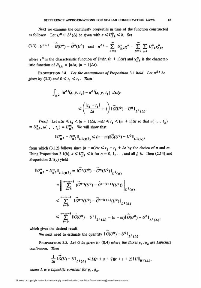
Next we examine the continuity properties in time of the function constructed
as follows: Let U° G Lx (A) be given with a < Ufk < b. Set
(3.3) U"+x=GiUn) = GniU°) and uAt = ¿ (7r2x" = ¿ £ V?.A>n=0 n=0 j,k
where x" is the characteristic function of [nAt, in + l)At) and x"k is the character-
istic function of Rj k x [77Ar, (n + l)Ar).
Proposition 3.4. Let the assumptions of Proposition 3.1 hold. Let uAt be
given by (3.3) and 0<tx <t2. Then
{ 2 \uAtix, y, t2) - uA\x, y, tx)\ dxdy
\U-tA \ -<M^+iW°)-,y<>llLi(A).
Proof Let «Ar < r2 < (« + l)Ar, mAt <tx <(m + l)At so that u(- ,-,t2)
= UR2,u(-, -, tx) = U™2. We will show that
11 Uh - "Ï2 W) < in - rn)\\G(U°) - Vi^,
from which (3.12) follows since (n - m)At <t2 - tx + At by the choice of tj and m.
Using Proposition 3.1(b), a < Ujik.< b for « = 0, 1,. . . and all /, k. Then (2.14) and
Proposition 3.1(c) yield
WR2-UR2hHR2)=Kn(U°)-Gm(U°AXiA)
n—m—l ->- -».£ (G"-'((70) - G"-(/+1 )(7y<>))
1=0 L!(A)
n—m—l ->- -*.
< £ II C"-'((70) - G"-('+ x \U°)\\r jf=o
¿1(A)
n—m—l ->■< V^ llr?777<h _ rrOg llG(C/°) - U°\\LX(A) = (n- m)\\GiU°) - £/°lLl(A),
which gives the desired result.
We next need to estimate the quantity llG(i/°) - U° ^Li,A)-
Proposition 3.5. Let G be given by (0.4) where the fluxes gx, g2 are Lipschitz
continuous. Then
¿ WGiU) - U\\LX(A)<Lip + q+2Xr + s + 2)\\U\\BV,A),
where L is a Lipschitz constant for gx, g2.
License or copyright restrictions may apply to redistribution; see https://www.ams.org/journal-terms-of-use
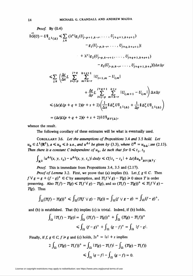
14 MICHAEL G. CRANDALL AND ANDREW MAJDA
Proof By (0.4)
^-u\\LX <Z (xxig1(t//_p+1)fc_r,..., Uj+q+Xtk+s+x)j,k
%liVj-p,k-n ■ ■ ■ ' Vj+q,k + s+l)\
A \S2iUj_pjc_r+x, . . . , Uj+q + xk+s+x)
-82ÍUj-P,k-r> ■■■> Uj+q+Xtk + s)\)AxAy
i + ° k + s+l\TT _ Tt
l,m<<Z (f¿ S Z loi«.«-»!/,* \ /=/-p m = k-r
At j+q+1 k+s \
+ £i Z Z lüi.m + l-^m'j^Ay"^ /=/-p m = k-r I
< (*)L<p + , 4 2)(7 + s + 2)(¿II A*+Í/IIl1(a) + ¿Il A^IILl(A)
= (Af)L(p +q + 2)(r + s+ 2)11 C/Hñr/(A),
whence the result.
The following corollary of these estimates will be what is eventually used.
Corollary 3.6. Let the assumptions of Propositions 3.4 and 3.5 hold. Let
u0 G LxiR2), a < u0 < b a.e., and uAt be given by (3.3), where U° = u0A ; see (2.13).
Then there is a constant C independent ofu0, At such that for 0 < tx, t2
Jr2 l«Aí(x,;p, r2) - uAí(x, ^ tx)\dxdy<a\tx-t2\+At)\\u0\\BV(R2y
Proof. This is immediate from Propositions 3.4, 3.5 and (2.17).
Proof of Lemma 3.2. First, we prove that (a) implies (b). Let/ g G C. Then
/ V g = g + (f - g)+ G C by assumption, and T(f V g) - T(g) > 0 since T is order
preserving. Also Tif) - 7fe) < 7{/ V *) - Tig), and so (l\f) - T(g))+ < Tif V g) -
Tig). Thus
SniTif) - T(g))+ < SaiTif Vg)- Tig)) = Sa(fVg-g) = fa(f-g)+.
and (b) is established. That (b) implies (c) is trivial. Indeed, if (b) holds,
/„ I Tif) - Tig)\ = /n (T(f) - T(g))+ + Jn (T(g) - Tif))+
Finally, iff, g G Ç f> g and (c) holds, 2s+ = Isl + s implies
2 /„ iTig) - Tif))+ = /„ I n?) - 7t/)l - /„ (7fe) - 7X/))
License or copyright restrictions may apply to redistribution; see https://www.ams.org/journal-terms-of-use
DIFFERENCE APPROXIMATIONS FOR SCALAR CONSERVATION LAWS 15
We have proved Lemma 3.2 here for completeness. The parallel result for L°°
and extensions are discussed in [5]. It is recognized that there will be results analo-
gous to those of this paper for, in particular, equations of the form ut - A^u) = 0
and ut + /(grad u) = 0; and, time permitting, these will be developed.
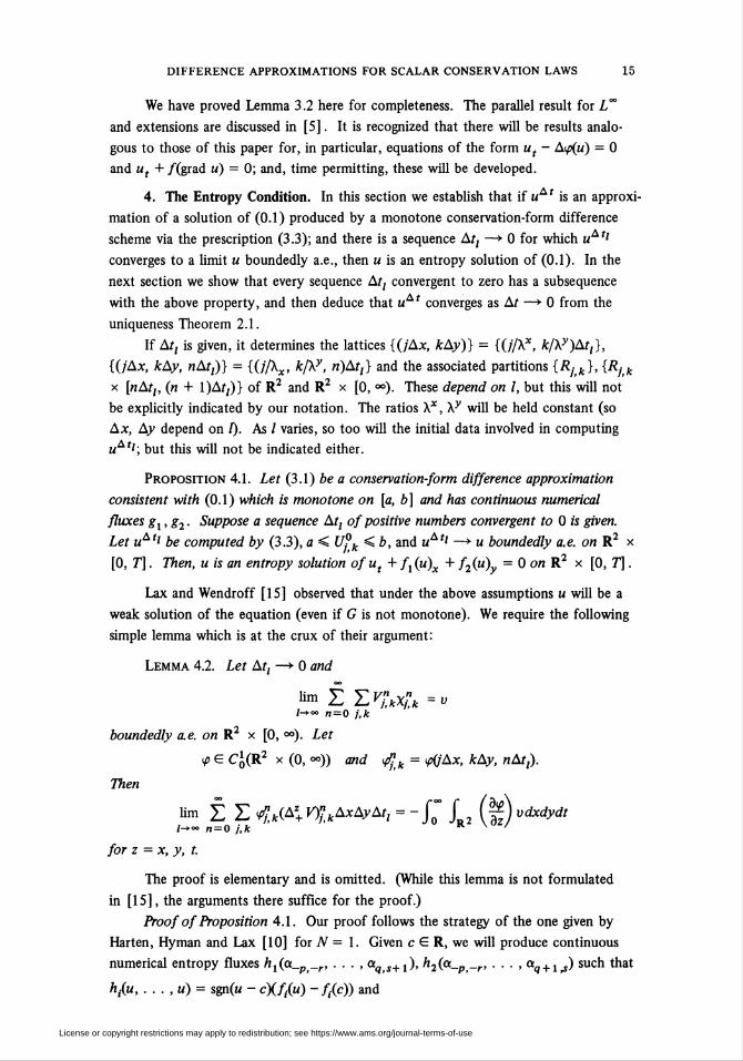
4. The Entropy Condition. In this section we establish that if uAt is an approxi-
mation of a solution of (0.1) produced by a monotone conservation-form difference
scheme via the prescription (3.3); and there is a sequence At¡ —► 0 for which uAtl
converges to a limit u boundedly a.e., then u is an entropy solution of (0.1). In the
next section we show that every sequence Ar, convergent to zero has a subsequence
with the above property, and then deduce that uAt converges as Ar —► 0 from the
uniqueness Theorem 2.1.
If Ar, is given, it determines the lattices {(/Ax, kAy)} = {iJ/Xx, k/Xy)At,},
{(/Ax, kAy, nAt,)} = Üj/Xx, k/Xy, n)At,} and the associated partitions {Rjik}, {R¡tk
x [nAt,, in + l)At,)} of R2 and R2 x [0, °°). These depend on I, but this will not
be explicitly indicated by our notation. The ratios X*, Xy will be held constant (so
Ax, Ay depend on f). As / varies, so too will the initial data involved in computing
uAtl; but this will not be indicated either.
Proposition 4.1. Let (3.1) be a conservation-form difference approximation
consistent with (0.1) which is monotone on [a, b] and has continuous numerical
fluxes gx,g2. Suppose a sequence At, of positive numbers convergent to 0 is given.
Let uAt{ be computed by (3.3), a < t/?fc < b, and uAt> —*■ u boundedly a.e. on R2 x
[0, T]. Then, u is an entropy solution of ut + fx (u)x + /2(w)y = 0 on R2 x [0, T].
Lax and Wendroff [15] observed that under the above assumptions u will be a
weak solution of the equation (even if G is not monotone). We require the following
simple lemma which is at the crux of their argument:
Lemma 4.2. Let At, —* 0 and
i™ ¿ZVj!kX^k=v/-><*> n=0 j,k
boundedly a.e. on R2 x [0, °°). Let
V? G C¿(R2 x (0, oo)) and tfk = tfjAx, kAy, nAt,).
Then
lim Z Z $k(A\VyiikAxAyAt, = - J" J (|) vdxdydt
for z = x,y, t.
The proof is elementary and is omitted. (While this lemma is not formulated
in [15], the arguments there suffice for the proof.)
Proof of Proposition 4.1. Our proof follows the strategy of the one given by
Harten, Hyman and Lax [10] for N = 1. Given c G R, we will produce continuous
numerical entropy fluxes hx(a_p_r, . . . , aq s+x), h2(a_p _r, . . . , aq + x >i) such that
h fit, ...,«) = sgn(w - cX/(«) -f((c)) and
License or copyright restrictions may apply to redistribution; see https://www.ams.org/journal-terms-of-use
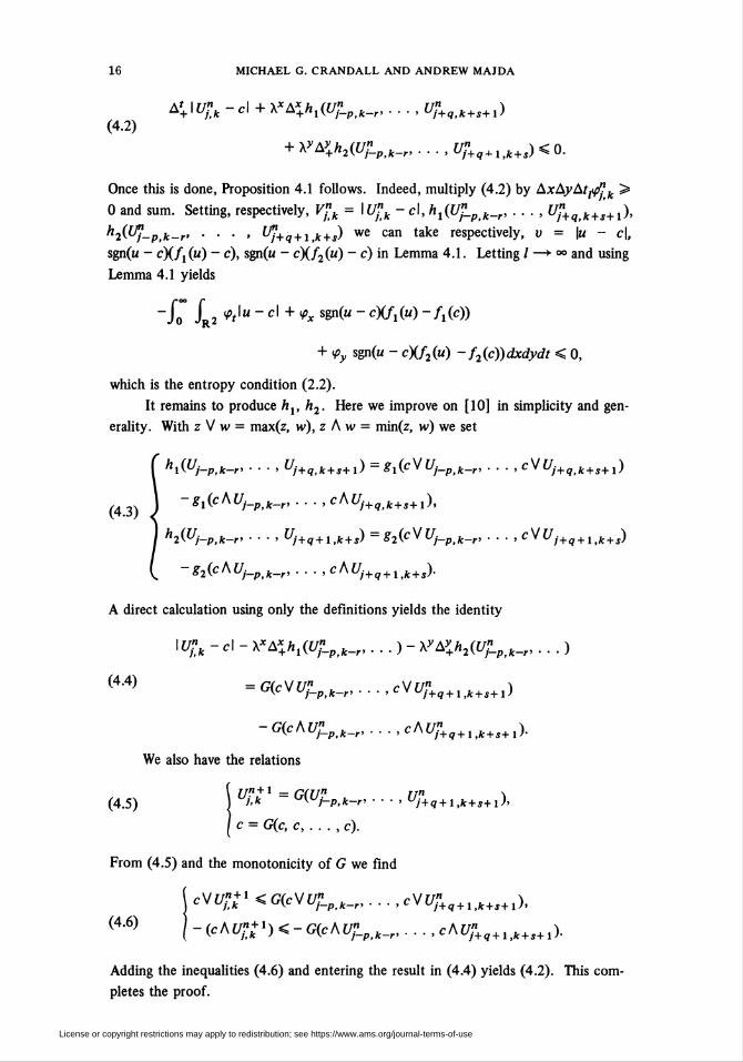
16 MICHAEL G. CRANDALL AND ANDREW MAIDA
A\\U?k-c\ + X'A**,^*.,, . . . , U?+qik + l+l)
(4.2)
+ XyAy+h2(U?_Ptk_r, ..., U¡-+q+x¡k+s) < 0.
Once this is done, Proposition 4.1 follows. Indeed, multiply (4.2) by AxAyAt,^k >
0 and sum. Setting, respectively, Vfk = \Ufik- c\, hx(Uj_pk_r, ..., Uf+qk+'s+x),
h2iTf}-p,k-r> ■ • • > ^f+q + i,k+s) we can take respectively, v = \u - c\,
sgn(« - c)ifx («) - c), sgn(« - c)(/2(«) - c) in Lemma 4.1. Letting / —► °° and using
Lemma 4.1 yields
~/o JR2 ^f1" ~c\+*x sgn(u - cX/,(w) ~fxic))
+ ipy sgn(« - cX/2(") - f2ic))dxdydt < 0,
which is the entropy condition (2.2).
It remains to produce «,, h2. Here we improve on [10] in simplicity and gen-
erality. With z V w = max(z, w), z Aw = min(z, w) we set
niiUj-p,k-r< • • • > ̂ /+<7,¡fc + .s-rl) = SlicVUj-p,k-r< • • • > C^ c7/+<7,fc + i-r l)
-giicAU^^,, . . -,cAUj+qk+s+x),
h2ÍUj-p,k-r> • • • ■ Uj+q + l,k + s)=g2ÍcS/Uj-p,k-r> ■■> C V f//+9 + 1 .* + ,)
-^(cAfJ^p^,. . . ,cA/7/+9+1>fc+,>.
A direct calculation using only the definitions yields the identity
\ufik - d - xxAx+hxiu»_p>k_r,. . . ) - xy Ay+h2iuf_Pik_r,...)
(4'4) = <**%,,*-.,cvu»+q+xtk+s+x)
-Gi^U»_Ptk_r,...,cAU?+q+Xtk + s+x).
We also have the relations
(4.5) \Uí-k = G(UhP,k-r' ■ ■ ■ >U"+q+l,k + s+l)'
| c = Gic c, . . . , c).
From (4.5) and the monotonicity of G we find
j c\/U»¿x<GicVU»_P:k_r, . . .,cVt/^ + u+s+1),
(4.6) I - (cAUn+x) <-GicAU" /-A/7" ï( ycnuj,k > *» <J\cnuj-p,k-r' ■ • ■ >cnuj+q+l,k + s+l>-
Adding the inequalities (4.6) and entering the result in (4.4) yields (4.2). This com-
pletes the proof.
License or copyright restrictions may apply to redistribution; see https://www.ams.org/journal-terms-of-use
DIFFERENCE APPROXIMATIONS FOR SCALAR CONSERVATION LAWS 17
5. The Proof of Theorem 1. We will actually prove more than Theorem 1 states
here, for we will not need to assume the existence of the solution Sit)uQ of (0.1).
This will follow from our proofs. To begin, we assume that a < m0 < b a.e., uQ G
BV(R2) and u0 has compact support. Let uAt be given by (3.3) with U° = u0A; see
(2.13).
From the stability estimates of Proposition 3.1 and (2.14)—(2.17) we deduce
(51) i l"Af("»">í)iz< l«o«z îorZ = Lx(R2), BV(R2), and
( a < uAt < b everywhere.
Also, because X*, Xy are fixed, it is easy to see that there is a c0 > 0 such that if «0
vanishes for Ixl + \y\> R, then
(5.2) uAt(x, y, t) = 0 for Ixl + \y\ >R + c0 + c0t, 0< Ai < 1.
Because bounded subsets of BV(R2) O LxiR2) are precompact in L¡ociR2) (see (2.9)),
(5.1) and (5.2) imply that if T> 0, then
(5.3) {uAti ■, ■, t) : 0 < t < T, 0 < Ai < 1} is precompact in LxiR2).
Next the estimate of Corollary 3.5 supplies us with
(5.4) H«Aí(-,-,í1)-«A,(-,-,í2)lli.1(R2)<c(lí1-í2l+2A0ll«0llBnR2).
By the proof of Arzela-Ascoli's theorem, (5.3) and (5.4) guarantee that if Ai, —► 0,
then there is a subsequence At,,k^ and a function u : [0, °°) —► LX(R2) such that
uAl
k-»» 0<t<T
From (5.1) and (5.4) we deduce a < u < b a.e. and
(5.6) H-,-,tx)-ui-,-,t2)\\LX(R2)<c\tx -i2llu0lBK(R2).
Passing to a further subsequence if necessary, we can have wA,'CO —► u boundedly a.e.
By Proposition 4.1, « is an entropy solution of the conservation law in (0.1). By (5.6),
and «( •, •, 0) = u0, u assumes the initial value u0 continuously in LxiR2). The
uniqueness Theorem 2.1 guarantees then the uniqueness of«, and we conclude
(5.7) lim IIuAti ■, •, t) - «( •, •, OH. i R2) = 0 uniformly for bounded t.it-»o l
This completes the analysis when «0 has compact support.
For general «0 G ¿'(R2) with a<u0<b a.e. we choose u0 m G BV(R2) Pi
LxiR2) with compact support such that
!d ^ "n m ^ b and
U"0-"0,m "¿Vr2)^0 aS772-^oo.
This can be done by any standard method. Denote the difference scheme solution cor-
responding to the initial-value u0 m by uAt. Below, we regard all functions as
functions of t with values in Lx (R2). We know that
(5.5) lim max \\uAt'(k\-, -, t) - «(•, •, t)\\7lfR2 = 0 forr>0.
License or copyright restrictions may apply to redistribution; see https://www.ams.org/journal-terms-of-use
18 MICHAEL G. CRANDALL AND ANDREW MAJDA
(5.9) Um uAtit) = umit) exists uniformly for bounded t.
At->0
Moreover, from Proposition 3.1(c) it follows that
sup ll«Ai(r) - uAt(í)ll i,r2) < H"o,m -"o,/llLi(R2)'f>0
and so {um } is Cauchy in C([0, °°) :Z,'(R2)) and hence converges uniformly to a
limit u G C([0, °°) :Z,'(R2)). Finally,
WuAtit)-uit)\\LX{K2)
< WuAtit)-uAtit)\\LX(R2) + ll«Ai(f)-«m(r)llil(R2) + ll»m(0-«(0llLl(R2)
< »«0 -"0,mllLl(R2) + »<f(0-«„(0«£l{RÎ) + l««(0-«C0\l(Ra)-
The first and third terms above can be made small uniformly in t by taking m large.
Then the middle term can be made small by taking At small (uniformly for t bounded).
Hence limAM.0 uAt = u locally uniformly in ¿'(R2) (and u is continuous into LxiR2)
by its construction). This completes the proof.
A reexarnination of the proof of Theorem 5.1 and the various ingredients of the
preceding sections shows that we have in fact proved the following results on existence
and properties of solutions of (0.1) (given the uniqueness Theorem 2.1).
Corollary 5.1. Let the conservation law have Lipschitz continuous fluxes f¡.
Then for every initial-data u0 GLxiRN) n ¿""(R^) there is a unique entropy solution
u G C([0, °°) ̂ (R^)) 0/(0.1) with u(0) = u0. Denoting this solution by Sit)uQ we
have:
(a) If u0 G BViRN), t —* Sit)u0 is Lipschitz continuous into LXÇRN) and
]^it)u0\\BV(KN)<\\u0\\BV(RNy
(b) \\Sit)u0 - Sit)VQ Hil(RiV) < ll«0 - V0 WLl(RNy
(c) u0 < v0 a.e. implies Sit)uQ < 5(r)u0 o.e.
id) a<u0 <b a.e. implies a < 5(r)«0 <b a.e.
All of the above is well known, even in much greater generality; see [13], in
particular. Crandall [4] and Benilan [1] also treat cases in which the f, need not be
Lipschitz. In fact, it is enough that the /• are continuous and
lim l/;.(r) -/•fC0)l/lrK7V-1>/JV = 0,r-*0
in order that Theorem 2.1 hold with ui0 G L°°(RN) n LX(RN), provided R = °° in
(2.3) and (2.4). In order to compute solutions of (0.1) in this non-Lipschitz case, one
would have to approximate (/.,..., fN) by smoother functions ifx, . . . , f^), solve
a difference approximation to the resulting problem with Xf, X^ chosen appropriate-
ly, and then let / —► °° , Ai —► 0. The modulus of continuity in time must be treated
appropriately, but we will not consider this here.
License or copyright restrictions may apply to redistribution; see https://www.ams.org/journal-terms-of-use
DIFFERENCE APPROXIMATIONS FOR SCALAR CONSERVATION LAWS 19
6. The Inhomogeneous Equation. We briefly remark on how the analysis given
above can be carried out for the more general problem
(6,) ,*+£■»*»****
u(x, 0) = H0(X).
The corresponding difference schemes have the form (for N = 2)
(6.2) U» + x = GiUf_Pik_r, ..., U?+q+ltk+s+l) + àtFj>k,
or
(6.3) {/»+i =~g\u") + AtF",
where G satisfies the conditions of the preceding sections.
Theorem 6.1. Let G define a conservation-form difference scheme consistent
with (0.1), which is monotone on [a, b] and has Lipschitz continuous fluxes. Let T
> 0, u0 G ¿~(R2) n LxiR2) andF£L°°(R2 x (0, T)) n LX(R2 * (0, T)) satisfy a
+ 71F0L«, <u0<b- \\F\\L<x,Ta.e. Let U° = u0A and
r?n _ 1 fin+1)At rFj,k - . . . A L Fix, y, t)dxdydt.
AtAxAyJnAt JRjtk v'-"
Then U", defined by (6.3) satisfies a < U? k < b for all n, j, k such that nAt < T and
«Af = Z Z t/M*n=0 j,k
converges in ¿'(R2) uniformly on compact subsets of [0, T) to the unique entropy
solution o/(6.1).
Sketch of Proof. In addition to the arguments in preceding sections we require
a uniqueness theorem (see [13] for this) and a few estimates given now. From Prop-
osition 3.1 we deduce immediately
Ísup Uf +x < sup Ufk + At sup Ffk,j,k
inf Up*x > inf Ufk + Ar inf Ffkj, k j, k j, k
and
(6.5) IIU" + x IIx < IIU" \\x + At IIF" \\x
for X = L'(A) and X = BV(A). Moreover, if Un+ x = G(U") + AtF", we find
(6.6) icr-f>uLl(A)< iii/o-i/0iiLl(A) + nf At\\F>-FnLl(Ay
Finally, the estimate of Proposition 3.4 is replaced (with n At < t2 < (n + l)At, m At
<tx <(m + l)At and m<nas before) by
License or copyright restrictions may apply to redistribution; see https://www.ams.org/journal-terms-of-use
20 MICHAEL G. CRANDALL AND ANDREW MAIDA
fR2\uAtix,y,t2)-uAtix,y,tx)\dt
n-l
\un-um\\T.,A< y \\uí+x -u'L.¿MA) .*-' L1
,=m
n-l
= £ HG(?y'') + ArF/'-ty''iiMj=m
lHa)
<"£ *GiU<)-un\ A+"£ At\\Fj\\Llj=m j=m
Now we use Proposition 3.5 and (6.5) to estimate the right-hand side above by
Atin - m) cons. (\\U°WBV(A) + £ At\\F'\\BV(A)) + Z Mfí1lUaY\ ¡=0 j j=m
Thus, if
\l\Fi-,-,f)\BVI^dt<~,
we have the type of equicontinuity of « 'as At —► 0 used in the proof of Theorem
1 ; and the proof may be completed much as before. (One begins, say, with u0 G
C^ÍR2), Fe CqÍR2 x [0, T)) and passes to the general case via (6.6).)
Mathematics Research Center
University of Wisconsin, Madison
Madison, Wisconsin S3706
Department of Mathematics
University of California, Berkeley
Berkeley, California 94720
1. PH. BENILAN, Equation d'Evolution dans un Espace de Banach Quelconque, Thesis,
Université de Orsay, 1972.
2. S. BURSTEIN, P. D. LAX & G. SOD, Lectures on Combustion Theory, Courant Mathe-
matics and Computing Laboratory Report, September 1978.
3. E. CONWAY & J. SMOLLER, "Global solutions of the Cauchy problem for quasilinear
first order equations in several space variables," Comm. Pure Appl. Math., v. 19, 1966, pp. 95—10S.
4. M. G. CRANDALL, "The semigroup approach to first order quasilinear equations in sev-
eral space variables," Israeli. Math., v. 12, 1972, pp. 108-132.
5. M. G. CRANDALL & L. TARTAR, "Some relations between non expansive and order
preserving mappings." (To appear.)
6. A. DOUGLIS, Lectures on Discontinuous Solutions of First Order Nonlinear Partial Dif-
ferential Equations in Several Space Variables, North British Symposium on Partial Differential
Equations, 1972.
7. N. DUNFORD & J. T. SCHWARTZ, Linear Operators, Part 1 : General Theory, Pure and
Appl. Math., Vol. 7, Interscience, New York, London, 1958.
8. S. K. GODUNOV, "Finite difference methods for numerical computations of discontin-
uous solution of equations of fluid dynamics," Afaf. Sb., v. 47, 1959, pp. 271-295. (Russian)
9. A. HARTEN, "The artificial compression method for computation of shocks and contact
discontinuities: I. Single conservation laws," Comm. Pure Appl. Math., v. 39, 1977, pp. 611-638.
10. A. HARTEN, J. M. HYMAN & P. D. LAX, "On finite difference approximations and
entropy conditions for shocks," Comm. Pure Appl. Math., v. 29, 1976, pp. 297-322.
License or copyright restrictions may apply to redistribution; see https://www.ams.org/journal-terms-of-use
DIFFERENCE APPROXIMATIONS FOR SCALAR CONSERVATION LAWS 21
11. G. JENNINGS, "Discrete shocks," Comm. Pure Appl. Math., v. 27, 1974, pp. 25-37.
12. K. KOJIMA, "On the existence of discontinuous solutions of the Cauchy problem for
quasilinear first order equations," Proc. lapan Acad., v. 42, 1966, pp. 705-709.
13. S. N. KRUZKOV, "First order quasilinear equations with several space variables,"
Math. USSR Sb., v. 10, 1970, pp. 217-243.
14. P. D. LAX, Hyperbolic Systems of Conservation Laws and the Mathematical Theory of
Shock Waves, SIAM Regional Conference Series in Applied Mathematics #11.
15. P. D. LAX & B. WENDROFF, "Systems of conservation laws," Comm. Pure Appl.
Math., v. 13, 1960, pp. 217-237.
16. A. Y. LE ROUX, "A numerical conception of entropy for quasi-linear equations,"
Math. Comp., v. 31, 1977, pp. 848-872.
17. A. MAJDA & M. CRANDALL, Numer. Math. (To appear.)
18. A. MAJDA & S. OSHER, "Numerical viscosity and the entropy condition," Comm.
Pure Appl. Math. (To appear.)
19. S. OHARU & T. TAKAHASHI, "A convergence theorem of nonlinear semigroups and
its application to first order quasilinear equations," J. Math. Soc. lapan, v. 26, 1974, pp. 124-160.
20. O. A. OLEINIK, "Discontinuous solutions of nonlinear differential equations," Amer.
Math. Soc. Transi. (2), v. 26, 1963, pp. 95-172.
21. G. STRANG, "On the construction and comparison of difference schemes," SIAM J.
Numer. Anal., v. 15, 1968, pp. 506-517.
22. A. I. VOL'PERT, "The spaces BV and quasilinear equations," Math. USSR Sb., v. 2,
1967, pp. 225-267.
23. N. N. KUZNECOV & S. A. VOLOSIN, "On monotone difference approximations for
a first-order quasi-linear equation," Soviet Math. Dokl., v. 17, 1976, pp. 1203 — 1206.
License or copyright restrictions may apply to redistribution; see https://www.ams.org/journal-terms-of-use