mohsen mohammed taqi mohsen al-saleh statistics-6000 · 18/11/2011 mohsen mohammed taqi mohsen...

18/11/2011 Mohsen Mohammed Taqi Mohsen Al-Saleh

Statistics-6000 Variable: are “characteristic that can take on different values” with respect to persons,

time, and place and types of variables are as follow:

Independent (X) you can choose and manipulate. Usually on x-axis

Dependent (Y) is what you measure in the experiment and what is affected during the experiment. Usually on y-axis

Intermediate is a variable in a causal pathway that causes variation in the dependent variable and is itself caused to vary by the independent variable

Confounder is an extraneous variable in a statistical model that correlates (positively or negatively) with both the dependent variable and the independent variable. The methodologies of scientific studies therefore need to account for these variables - either through true experimental designs, in which case, one achieves control, or through statistical means. (Internal Validity)

Discrete Variable: This is a whole number and countable variable. Ordinal, Ranking Type or Nominal Classificatory Categorical Type. (qualitative variable)

Continuous or measurable variable: variables have no gaps between them. Have

decimal points and units. (Quantitative variable)

Why statistic in general: collection of data, summarization and analyzing of data set, evaluation, conduct a research and finally making conclusion (Testing hypothesis)

Specific goal of statistic: define a normal range (μ and σ), correlation study

(relationship), regression study (prediction), association (Qui-Square Test) & agreement testing (Cronblach Alpha & Kappa Cohen Correlation), testing hypothesis (z,t,f) and quality control (L G Chart)

Sample (n): small random group of individuals or observations that is chosen for study

from population. Sample is a part of population.

Random sample: is the selection of the sample such that every member from the population has an equal chance of being included in the sample


Sampling unit: A part from population, an individual, household, school, section, village Sampling frame: a complete list of sampling units in the population Why we need sample study:

o Less time o Less personnel o Less resources o Less money o For in-depth study

Sample size: the number of individuals or observations under study. (n≥ 30) Sampling methods:

o Simple Random Sampling: Each unit in this method has an equal probability of

being included in the sample. (Lottery sample) by using tables of random numbers. Is used when there is homogeneity in the study elements of the population. (N) is small

o Stratified Sampling: The study elements of population are heterogeneous. (N) is lager. (Stratum). Precision (1/SE) of the estimate will be high (SE will be less)

o Systematic Sampling (convenience): (N) is very large. (K)=N/n; is sampling interval. One number (X) is chosen randomly from (1 to K). X+0K, X+1K, X+2K X+3K… , X+ (n-1) K are included in the sample. Precision of the estimate will be less.

o Cluster Sampling: (N) is large and it’s not possible to get complete listing of the population unit. Precision of the estimate will be less.

o Multi Stage Sampling: (N) is very large. Sampling is done in stages. Precision of the estimate will be less.

o Quota Sampling: (Sampling of Convenience). (n) Is fixed and not probability sampling method. Not randomly selected. Results cannot be generalized but applicable to that area only. Not good sampling method.

Population (N): Aggregate of subjects under consideration. Whole group is representative

Parameters (μ and σ) ≠ Statistics ( and SD or s)

Statistical methods: descriptive method and inference method


Descriptive method: frequency tables, diagrams, graphs (bar chart, pie chart, pictogram, histogram, frequency polygon and curves-linerity), arithmetic or geometric or weighted mean, median, mode, range, quartile deviation(IQR), mean deviation, standard deviation(SD), coefficient of variation (CV%), correlation coefficient (r)-Pearson Product Moment Correlation, and regression analysis used for predication.

Inference analysis: used to generalize the results, obtained from the random sample, for

the population from which the representative sample was selected. Two main components of inference method are:

Estimation of Parameters (population values) Testing the Statistical Significance of the Hypothesis

Measure of location: mean, mode, and median. They are one single value to represent

the distribution. When these values describe a population they called parameters. If the describe a sample then referred as statistic(s).

Mean ( or µ) = ∑풙풏

or ∑풙푵

مجموع القیم على العدد

Median: is the middle most value of the arrange data set (continuous distribution). The value of it is not affected by the extreme values and therefore median is preferred to mean when there are extreme values. When sample not normally distributed

Mode: the most frequent observation of data/distribution. Distribution may have more

than 1 mode.

There are 2 types of data? Group data and Un-group data (very rich)

Why we group the data? Grouping the actual data collected will lose enrichment of the data set from its actual values but some time we need to hide the actual data from the public and other competitors or for simplification of data we handing large data set.

∑f = n or N ; total number of frequency = number of observations (sample size)

Number of classes or groups needed to make histogram: 2k ≥ n or N

Class Interval Size = 푴풂풙풊풎풖풎 푴풊풏풊풎풖풎

풌; this is increment value that would be added

For group data arithmetic mean; = ∑풎풇

∑풇 , where (m = mid-value of class interval)


Mid-value = (Lower limit:L1 + Upper limit:L2) ÷ 2; these L = real limits only

∑(x- ) = Zero, always

Variance for a group data; (SD2 or σ2) = ∑풇풎ퟐ

∑풇− ퟐ

While computing arithmetic mean for a given grouped frequency distribution, it is

assumed that all values falling in a particular group or class are located at the mid-point of the group.

For group median= L1 +

푳ퟐ 푳ퟏ풇

풙 푵ퟐ− 푪 , f = median frequency, C=cumulative fre.

Law of “next”

If the given class limits are “score limits” then convert them to “real limits”

Last group of cumulative frequency = N or n or ∑f

For group mode = L1 + 푳ퟐ 푳ퟏ

ퟐ풇 풇ퟏ 풇ퟐ 풙 (풇 − 풇ퟏ) ; class with maximum frequency

Quartiles and Percentiles: are the values in the continuous distribution showing the

proportion/percentage of lying below (or up to) the given value

Qi = L1 + 푳ퟐ 푳ퟏ풇

x 풊 풙 푵ퟒ− 푪 ; i = 1,2,3 (looks very likely to median formula)

Interquartile range (IQR): reflects the variability among the middle 50% of the

observation of the data. Better than range ( uses extreme values only)

Q1 (25%) and Q2 (50%) and Q3 (75%)

IQR = Q3 – Q1 ; better than ‘range’ = 75%-25%=50%

P50 = Q2 = Median; of continuous data distribution

Real times limits used for group data for: median, mode, quartiles, and percentiles


Pi = L1 + 푳ퟐ 푳ퟏ풇

x 풊 풙 푵ퟏퟎퟎ

− 푪 ; i = 1,2,3,….,99 (looks very likely to median formula)

Rule of “next” to locate the class interval from cumulative frequency distribution

Measure of Variability = Range, IQR, Variance, SD, and Coefficient of Variation

Measure of Variability = Scatter or dispersion of data around the mean

Range = Largest observation – Smallest observation

σ2= ∑(푿 흁)ퟐ

푵 or SD2 = ∑(풙 )ퟐ

풏 ퟏ ; variance of ungroup data

Group data σ2 or SD2 = ∑풙ퟐ

풏 ퟏ− (∑풙)ퟐ

풏(풏 ퟏ); no need for

= ∑풇풎∑풇

σ or SD = + 훔ퟐ퐨퐫 퐒퐃ퟐ ; unit of SD is similar to observation value

CV = 퐒퐃 퐱 ퟏퟎퟎ ; no unit its unitless quantity

CV% is used to compare variation between same sample variables or different

An event = outcome

Probability of (A) = is the proportion of times the outcomes would occur in a very long

series of repetitions. (all events are equally likely)

P(A) = 풎풏

(0 ≤m≤ 풏); when (n) is exhaustive, mutually exclusive

Equally likely trials of (m) is possible


Independent events: two events are said to be independent if the presence or absence of one does not alter the chances of the other being present, or of the occurrence of one does not alter the chance of occurrence of the other. (means that they can occur together)

Mutually exclusive events: if they cannot both occur together or be present at the same

time. No overlapping between the outcomes. Coins flipping head or tail

Additive rule: mutually exclusive events – the probability of occurrence of 2 or more mutually exclusive events is the sum of their probabilities of each outcome

P (A or B) = P (A) + P (B) e.g. throwing die for odd numbers- mutually exclusive ev.

Multiplicative rule: Independent events – probability of simultaneous occurrence of

events A and B in a series of independent trails (i.e. chance of one outcome occurring is not affected by knowledge of whether or not the other occurred) is the product of their probabilities.

P (A and B) = P(A) x P(B)→Independent events

General additive rule: if the 2 events are not mutually exclusive, then the probability

that either event A or B occurs is: P(A or B or both) = P(A) + P(B) – P(A & B)

Discrete Probability Distribution (DPD): sum of p(x)s = 1, probability of each outcome is between 0-1, outcomes are mutually exclusive.

μ=∑(xi p(xi)) and σ2 =∑((퐱퐢 − 흁)ퟐ.풑(풙풊)) ; for discrete probability distribution

Conditional probability:

Joint probability: P(A∩B)= P(A) x P(B) = multiplicative rule

Binomial Distribution: have two outcomes only one or zero. Its discrete distribution

p(x) = 퐶 푝 푞 ; 퐶 is called binomial coefficient. (0 ≤ x ≤ n)

C =1 and C = 1 and 0! = 1 and (p+q)n = 1; p is the parameters and n is the degree of

binomial distribution and n and p is fixed, trails independent, 2 outcomes possible


Its application when population is dichotomized or divided into 2 classes only

(p) is the probability of success and (q) is the probability of failure. (p+q)=1

The mean of the binomial distribution (expected value) = p(x) = mean = n p

The variance of binomial distribution V(x) or σ2 = n p q; if n.p.q ≥ 10 we can use

normal distribution to approximate binomial

At least to 10 = P(10≤x≤n) = in the questions

At most to 10 = P(0≤x≤10) = in the questions

At least one will return: 1-p(x=0) in the binomial distribution = in the questions

The Poisson distribution: discrete distribution, trails are independent, p is very small, n is very large, events are very rare.

P(x) = 풙

풏

P(x) = 풆흀 흀풙

풙!; x=0, 1, 2,…….∞. λ (Aver.)= n.p; is parameters (Mean = Variance)

e=2.7183

Normal distribution: for continuous distribution, large number of observations, curve is

bell-shaped, symmetrical about the mean, mean=mode=median, total area under the curve = 1sqr unit and it approximate the histogram (frequency polygon).

The mean of all possible sample mean is equal to the population mean, therefore sample mean is called unbiased estimation of population.


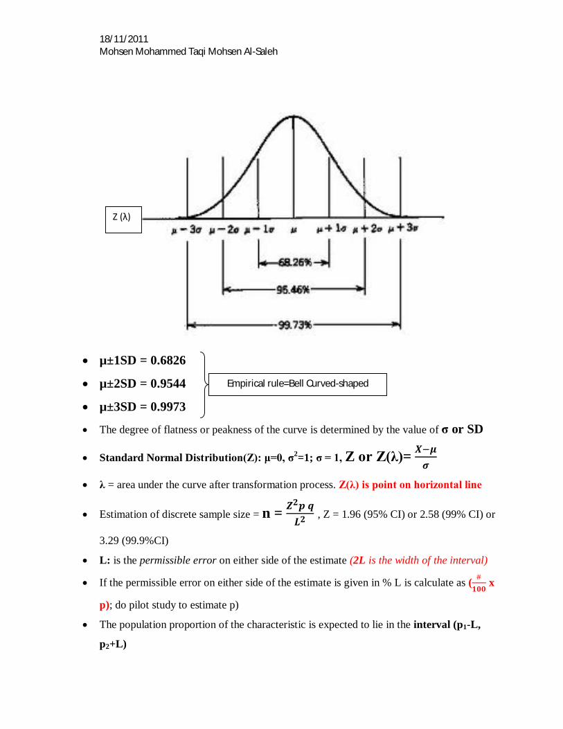
µ±1SD = 0.6826

µ±2SD = 0.9544

µ±3SD = 0.9973

The degree of flatness or peakness of the curve is determined by the value of σ or SD

Standard Normal Distribution(Z): μ=0, σ2=1; σ = 1, Z or Z(λ)= 푿 흁흈

λ = area under the curve after transformation process. Z(λ) is point on horizontal line

Estimation of discrete sample size = n = 풁ퟐ풑 풒푳ퟐ

, Z = 1.96 (95% CI) or 2.58 (99% CI) or

3.29 (99.9%CI)

L: is the permissible error on either side of the estimate (2L is the width of the interval)

If the permissible error on either side of the estimate is given in % L is calculate as ( #ퟏퟎퟎ

x

p); do pilot study to estimate p)

The population proportion of the characteristic is expected to lie in the interval (p1-L,

p2+L)

Z (λ)

Empirical rule=Bell Curved-shaped


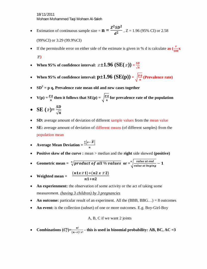
Estimation of continuous sample size = n = 풁ퟐ푺푫ퟐ

풅ퟐ , Z = 1.96 (95% CI) or 2.58

(99%CI) or 3.29 (99.9%CI)

If the permissible error on either side of the estimate is given in % d is calculate as ( #ퟏퟎퟎ

x

)

When 95% of confidence interval: ±1.96 (SE( )) = 푺푫√풏

When 95% of confidence interval: p±1.96 (SE(p)) = 풑.풒풏

(Prevalence rate)

SD2 = p q, Prevalence rate mean old and new cases together

V(p) = 풑.풒풏

then it follows that SE(p) = 풑.풒풏

for prevalence rate of the population

SE ( )= 푺푫√풏

SD: average amount of deviation of different sample values from the mean value

SE: average amount of deviation of different means (of different samples) from the

population mean

Average Mean Deviation = ∑ 풙

풏

Positive skew of the curve : mean > median and the right side skewed (positive)

Geometric mean = 풑풓풐풅풖풄풕 풐풇 풂풍풍 % 풗풂풍풖풆풔풏 or = 풗풂풍풖풆 풂풕 풆풏풅풗풂풍풖풆 풂풕 풃풆품풊풏품

풏 − ퟏ

Weighted mean = (풏ퟏ풙 ퟏ) (풏ퟐ 풙 ퟐ)

풏ퟏ 풏ퟐ

An experienment: the observation of some activity or the act of taking some

measurement. (having 3 children) by 3 pregnancies

An outcome: particular result of an experiment. All the (BBB, BBG…) = 8 outcomes

An event: is the collection (subset) of one or more outcomes. E.g. Boy-Girl-Boy

A, B, C if we want 2 joints

Combinations (푪풓풏)= 풏!(풏 풓)! 풓!

- this is used in binomial probability: AB, BC, AC =3


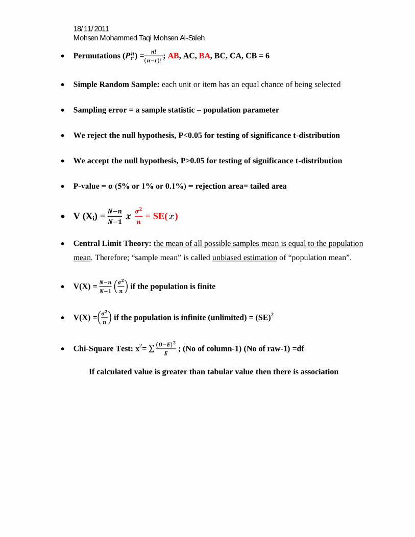
Permutations (푷풓풏) = 풏!(풏 풓)!

; AB, AC, BA, BC, CA, CB = 6

Simple Random Sample: each unit or item has an equal chance of being selected

Sampling error = a sample statistic – population parameter

We reject the null hypothesis, P<0.05 for testing of significance t-distribution

We accept the null hypothesis, P>0.05 for testing of significance t-distribution

P-value = α (5% or 1% or 0.1%) = rejection area= tailed area

V (Xi) = 푵 풏푵 ퟏ

풙 흈ퟐ

풏 = SE( )

Central Limit Theory: the mean of all possible samples mean is equal to the population

mean. Therefore; “sample mean” is called unbiased estimation of “population mean”.

V(X) = 푵 풏푵 ퟏ

흈ퟐ

풏 if the population is finite

V(X) = 흈ퟐ

풏 if the population is infinite (unlimited) = (SE)2

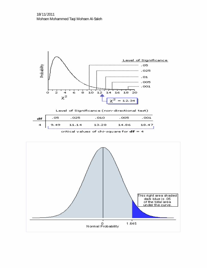
Chi-Square Test: x2= ∑ (푶 푬)ퟐ

푬 ; (No of column-1) (No of raw-1) =df

If calculated value is greater than tabular value then there is association


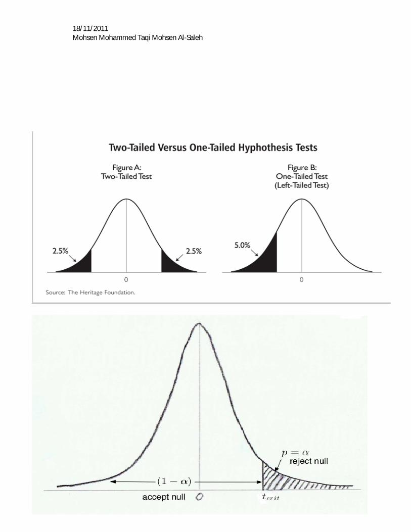
One-tailed t-test; H0=0 and H1 > 0 or H1 < 0


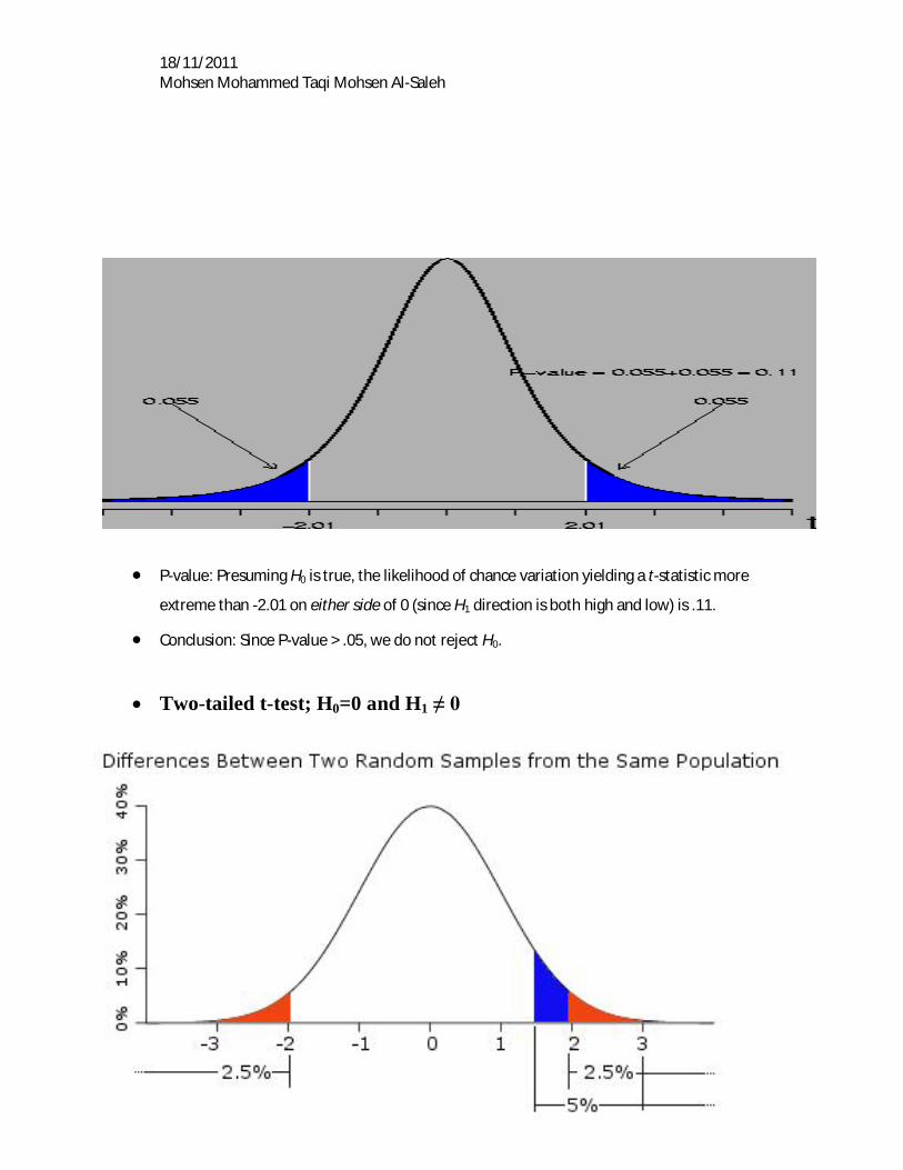
P-value: Presuming H0 is true, the likelihood of chance variation yielding a t-statistic more

extreme than -2.01 on either side of 0 (since H1 direction is both high and low) is .11.

Conclusion: Since P-value > .05, we do not reject H0.

Two-tailed t-test; H0=0 and H1 ≠ 0


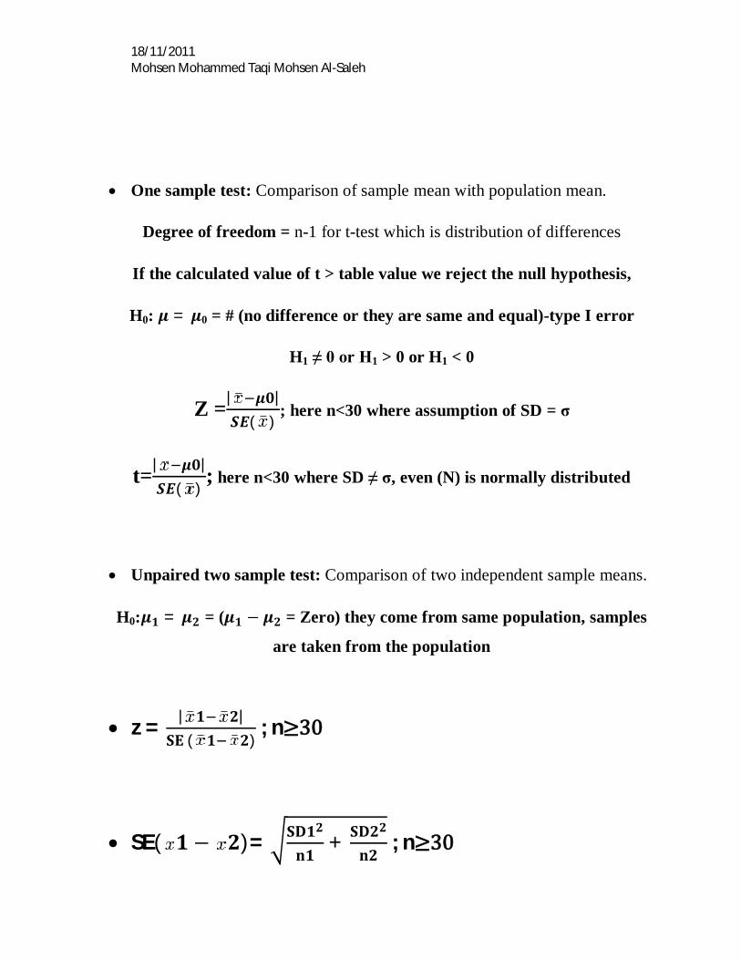
One sample test: Comparison of sample mean with population mean.

Degree of freedom = n-1 for t-test which is distribution of differences

If the calculated value of t > table value we reject the null hypothesis,

H0: 흁 = 흁0 = # (no difference or they are same and equal)-type I error

H1 ≠ 0 or H1 > 0 or H1 < 0

Z =| 흁ퟎ|푺푬( )

; here n<30 where assumption of SD = σ

t=| 흁ퟎ|푺푬( )

; here n<30 where SD ≠ σ, even (N) is normally distributed

Unpaired two sample test: Comparison of two independent sample means.

H0:흁ퟏ = 흁ퟐ = (흁ퟏ − 흁ퟐ = Zero) they come from same population, samples

are taken from the population

z = | ퟏ ퟐ|

퐒퐄 ( ퟏ ퟐ) ; n≥30

SE( ퟏ − ퟐ)= 퐒퐃ퟏퟐ

퐧ퟏ+ 퐒퐃ퟐퟐ

퐧ퟐ ; n≥30


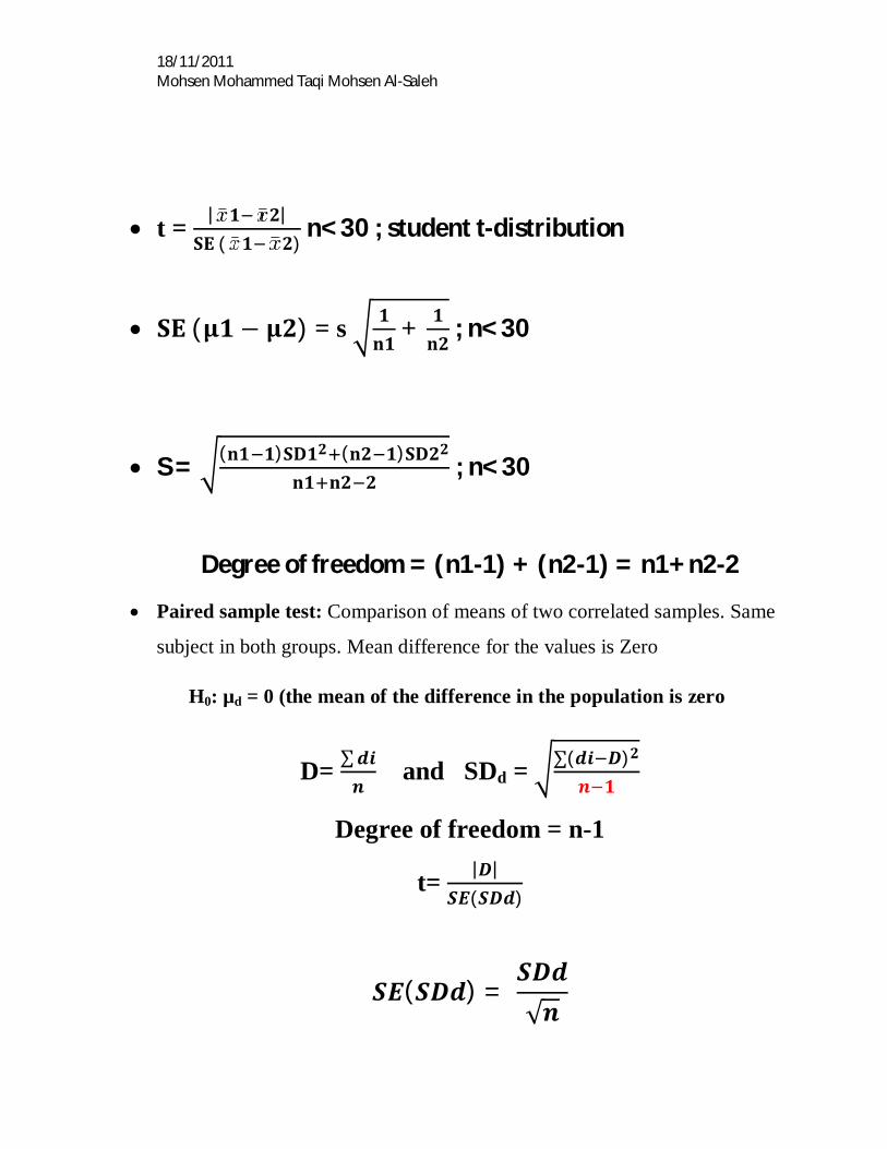
t = | ퟏ ퟐ|퐒퐄 ( ퟏ ퟐ)

n<30 ; student t-distribution

퐒퐄 (훍ퟏ − 훍ퟐ) = s ퟏ퐧ퟏ

+ ퟏ퐧ퟐ

; n<30

S = (퐧ퟏ ퟏ)퐒퐃ퟏퟐ (퐧ퟐ ퟏ)퐒퐃ퟐퟐ

퐧ퟏ 퐧ퟐ ퟐ ; n<30

Degree of freedom = (n1-1) + (n2-1) = n1+n2-2

Paired sample test: Comparison of means of two correlated samples. Same

subject in both groups. Mean difference for the values is Zero

H0: µd = 0 (the mean of the difference in the population is zero

D= ∑풅풊풏

and SDd = ∑(풅풊 푫)ퟐ

풏 ퟏ

Degree of freedom = n-1

t= |푫|푺푬(푺푫풅)

푺푬(푺푫풅) = 푺푫풅√풏


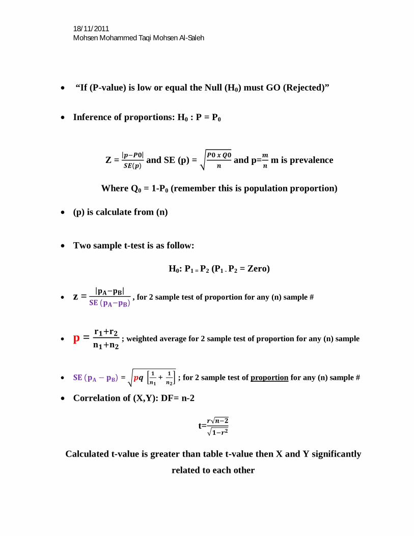
“If (P-value) is low or equal the Null (H0) must GO (Rejected)”

Inference of proportions: H0 : P = P0

Z = |풑 푷ퟎ|푺푬(풑)

and SE (p) = 푷ퟎ 풙 푸ퟎ풏

and p=풎풏

m is prevalence

Where Q0 = 1-P0 (remember this is population proportion)

(p) is calculate from (n)

Two sample t-test is as follow:

H0: P1 = P2 (P1 - P2 = Zero)

z = |퐩퐀 퐩퐁|퐒퐄 (퐩퐀 퐩퐁)

, for 2 sample test of proportion for any (n) sample #

p = 퐫ퟏ 퐫ퟐ퐧ퟏ 퐧ퟐ

; weighted average for 2 sample test of proportion for any (n) sample

퐒퐄 (퐩퐀 − 퐩퐁) = 풑풒 ퟏ풏ퟏ

+ ퟏ풏ퟐ

; for 2 sample test of proportion for any (n) sample #

Correlation of (X,Y): DF= n-2

t=풓√풏 ퟐ

ퟏ 풓ퟐ

Calculated t-value is greater than table t-value then X and Y significantly

related to each other


Regression: a=is the y-intercept and b=slope

Y= a + bX

Percentage of total variation in Y explained by X = 100 (r)2

t= 퐫∗√퐧 ퟐ

ퟏ 퐫ퟐ if t(calculated) > t(table) then variables (X,Y) related to each other

mohsen mohammed taqi mohsen al-saleh statistics-6000 · 18/11/2011 mohsen mohammed taqi mohsen...

Documents