module 1. classical vs machine learning econometrics · overview of classical econometrics what is...
TRANSCRIPT

Eurostat
THE CONTRACTOR IS ACTING UNDER A FRAMEWORK CONTRACT CONCLUDED WITH THE COMMISSION
Module 1. Classical vs machine learningeconometrics

Eurostat
2
▪ Overview of classical econometrics:
➢ What is econometrics
➢ Multiple regression
➢ Time series
▪ Econometric methods in Official statistics
▪ Models of inference

Eurostat
1. What is econometrics
Eurostat
4
Overview of classical econometrics
What is econometrics
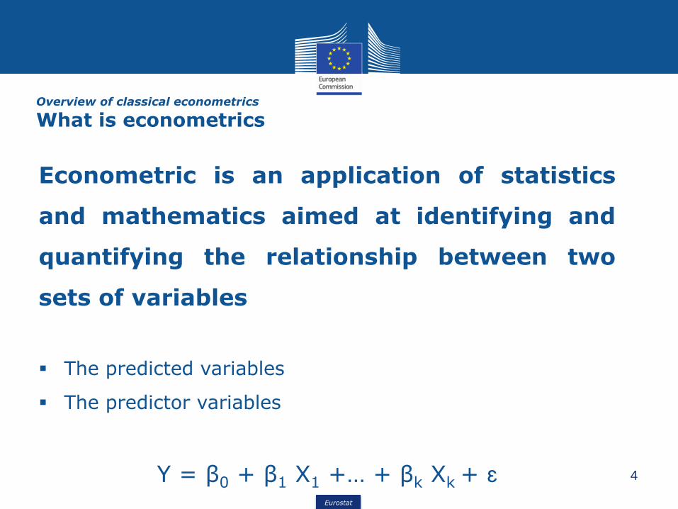
Econometric is an application of statistics
and mathematics aimed at identifying and
quantifying the relationship between two
sets of variables
▪ The predicted variables
▪ The predictor variables
Y = β0 + β1 X1 +… + βk Xk + ɛ
Eurostat
5
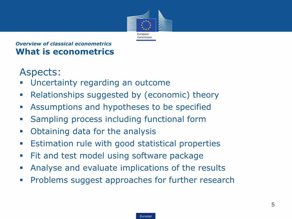
Aspects:▪ Uncertainty regarding an outcome
▪ Relationships suggested by (economic) theory
▪ Assumptions and hypotheses to be specified
▪ Sampling process including functional form
▪ Obtaining data for the analysis
▪ Estimation rule with good statistical properties
▪ Fit and test model using software package
▪ Analyse and evaluate implications of the results
▪ Problems suggest approaches for further research
Overview of classical econometrics
What is econometrics
Eurostat
6
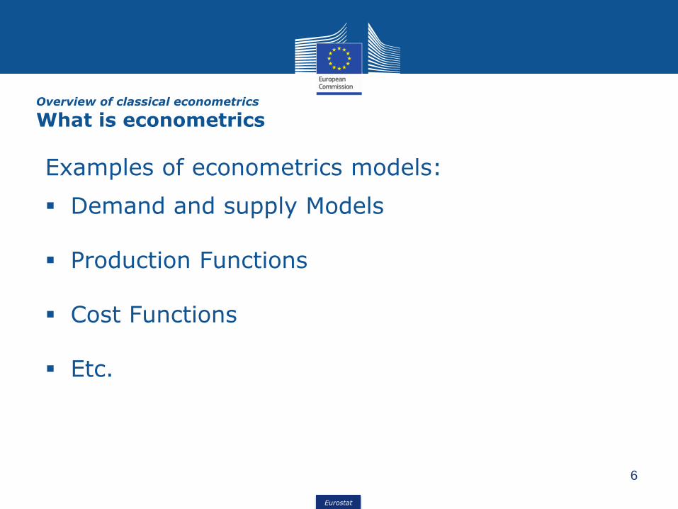
Examples of econometrics models:
▪ Demand and supply Models
▪ Production Functions
▪ Cost Functions
▪ Etc.
Overview of classical econometrics
What is econometrics
Eurostat
7
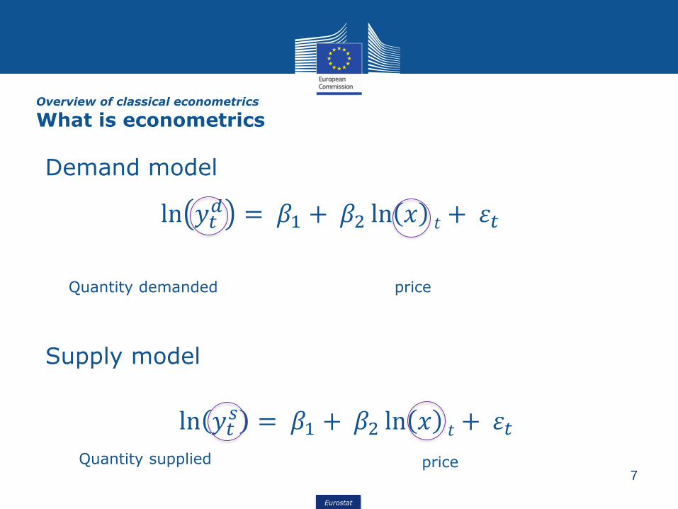
Demand model
Overview of classical econometrics
What is econometrics
ln 𝑦𝑡𝑑 = 𝛽1 + 𝛽2 ln 𝑥 𝑡 + 휀𝑡
Quantity demanded price
Supply model
ln 𝑦𝑡𝑠 = 𝛽1 + 𝛽2 ln 𝑥 𝑡 + 휀𝑡
Quantity supplied price
Eurostat
8
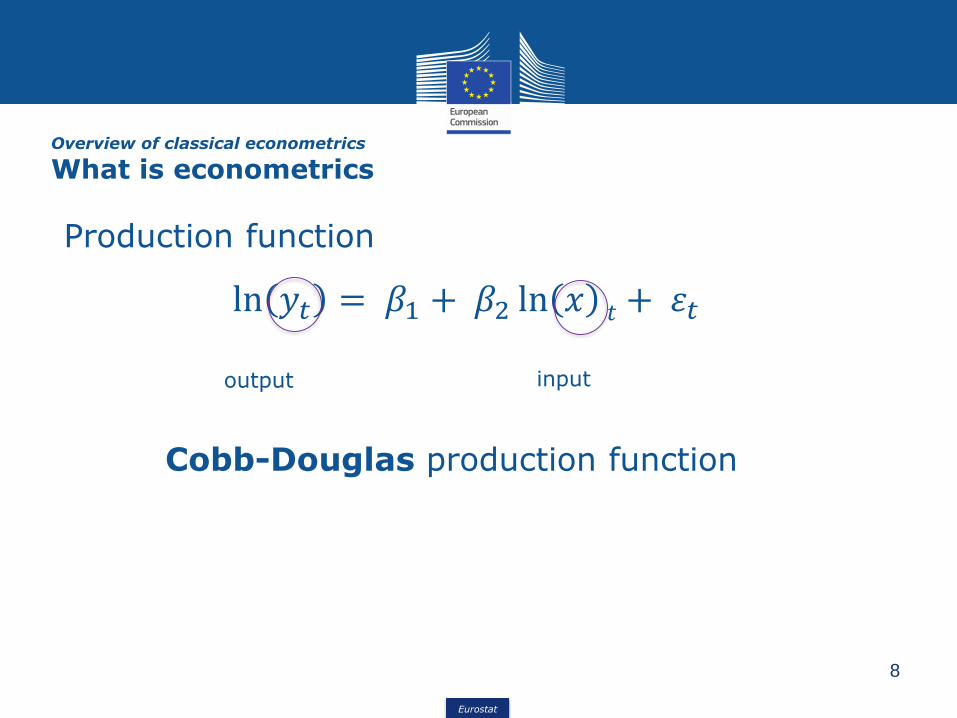
Production function
Overview of classical econometrics
What is econometrics
ln 𝑦𝑡 = 𝛽1 + 𝛽2 ln 𝑥 𝑡 + 휀𝑡
output input
Cobb-Douglas production function
Eurostat
9
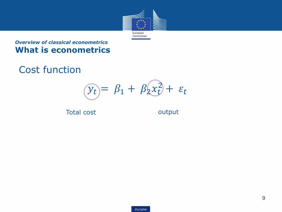
Cost function
Overview of classical econometrics
What is econometrics
𝑦𝑡 = 𝛽1 + 𝛽2𝑥𝑡2 + 휀𝑡
Total cost output
Eurostat
10
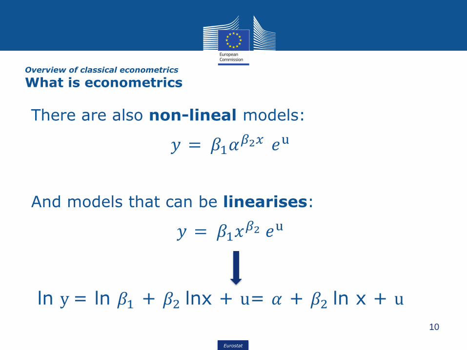
There are also non-lineal models:
𝑦 = 𝛽1𝛼𝛽2𝑥 𝑒u
And models that can be linearises:
𝑦 = 𝛽1𝑥𝛽2 𝑒u
Overview of classical econometrics
What is econometrics
ln y= ln 𝛽1 + 𝛽2 lnx + u= 𝛼 + 𝛽2 ln x + u
Eurostat
2. The multiple linear regression model
Eurostat
12
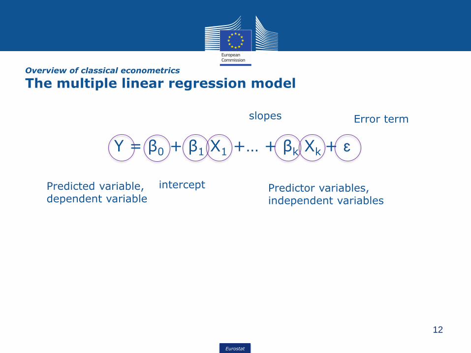
Y = β0 + β1 X1 +… + βk Xk + ɛ
Overview of classical econometrics
The multiple linear regression model
Predicted variable, dependent variable
Predictor variables, independent variables
intercept
slopes Error term
Eurostat
13
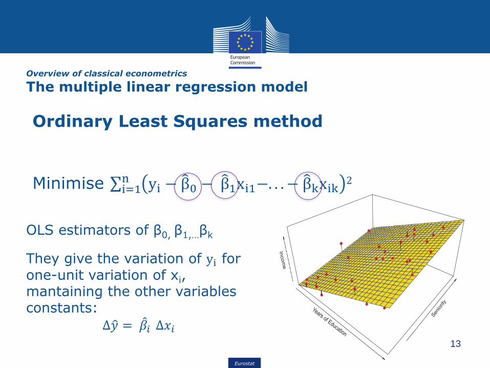
Ordinary Least Squares method
Minimise σi=1n yi − β0 − β1xi1−. . . − βkxik
2
Overview of classical econometrics
The multiple linear regression model
OLS estimators of β0, β1,…βk
They give the variation of yi for one-unit variation of xi, mantaining the other variables constants:
Δො𝑦 = መ𝛽𝑖 Δ𝑥𝑖
Eurostat
14
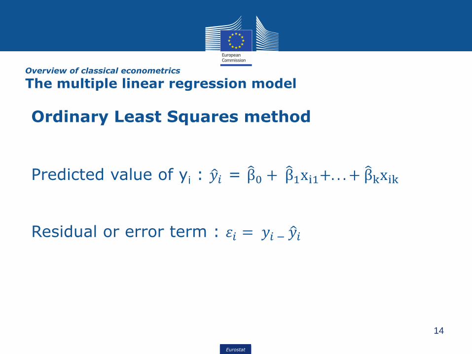
Ordinary Least Squares method
Predicted value of yi : ො𝑦𝑖 = β0 + β1xi1+. . . + βkxik
Residual or error term : 휀𝑖 = 𝑦𝑖 − ො𝑦𝑖
Overview of classical econometrics
The multiple linear regression model

Eurostat
15
Assumptions:
▪ E(휀𝑖|Xi) = 0 휀𝑖 has conditional zero mean
▪ (Xi,Yi) i.i.d i=1,..n
▪ Xi and 휀𝑖 have nonzero finite fourth moment
▪ There is no perfect multicollinearity (see later)
▪ var(휀𝑖|Xi) = 𝜎𝜀2 homoschedasticies
▪ The conditional distribution of 휀𝑖 given Xi is normal
Overview of classical econometrics
The multiple linear regression model
Eurostat
16
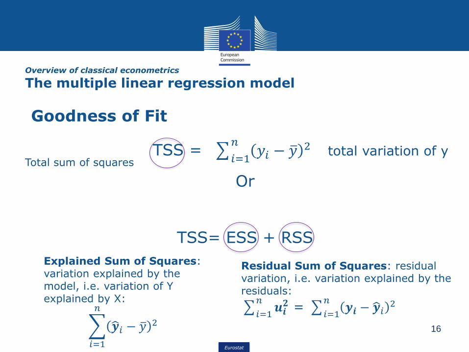
Goodness of Fit
TSS = 𝑖=1
𝑛𝑦𝑖 − ത𝑦 2 total variation of y
Or
TSS= ESS + RSS
Overview of classical econometrics
The multiple linear regression model
Total sum of squares
Explained Sum of Squares: variation explained by themodel, i.e. variation of Y explained by X:
𝑖=1
𝑛
ෝ𝒚𝑖 − ത𝑦 2
Residual Sum of Squares: residual variation, i.e. variation explained by theresiduals:
𝑖=1
𝑛𝒖𝒊𝟐 =
𝑖=1
𝑛𝒚𝒊 − ෝ𝒚𝑖
2

Eurostat
17
Goodness of Fit
R2= 𝐄𝐒𝐒
𝐓𝐒𝐒0≤ R2 ≤ 1
It can also be written as 1 –𝐑𝐒𝐒
𝐓𝐒𝐒
Adjusted R2 = 1-𝑛−1
𝑛−𝑘(1- R2)
Overview of classical econometrics
The multiple linear regression model
Eurostat
18
Overview of classical econometrics
Collinearity
▪ The term “independent variable” means anexplanatory variable is independent of theerror term, but not necessarily independentof other explanatory variables.
▪ Since economists typically have no control overthe implicit “experimental design”, explanatoryvariables tend to move together which oftenmakes sorting out their separate influencesrather problematic.
Eurostat
19
Overview of classical econometrics
Collinearity
Evidence of high collinearity include:
▪ a high pairwise correlation between twoexplanatory variables
▪ a high R-squared when regressing oneexplanatory variable at a time on each of theremaining explanatory variables
▪ a statistically significant F-value when thet-values are statistically insignificant
▪ an R2 that doesn’t fall by much when droppingany of the explanatory variables
Eurostat
20
Overview of classical econometrics
Collinearity
▪ Collinearity doesn’t mean the model ismisspecified
▪ Especially common problem in time seriesregressions
▪ It depends on lack of adequate information in thesample
Eurostat
21
Overview of classical econometrics
Collinearity
Some solutions:
➢ collect more data with better information
➢ impose economic restrictions as appropriate
➢ impose statistical restrictions when justified
➢ if all else fails at least point out that the poormodel performance might be due to thecollinearity problem (or it might not).

Eurostat
3. Time series models
Eurostat
23
Overview of classical econometrics
Time series models
A collection of observations madesequentially in time (stochastic process)
Examples:- Unemployment rate over time- Inflation rate - Production indices- Number of deaths/births- Etc.
Eurostat
24
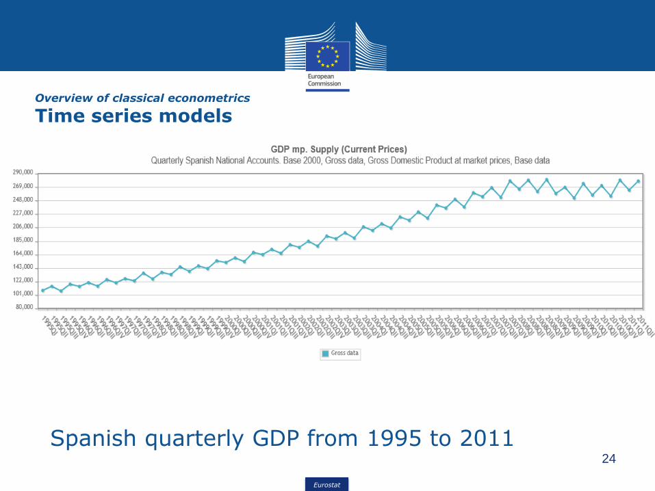
Overview of classical econometrics
Time series models
Spanish quarterly GDP from 1995 to 2011

Eurostat
25
Overview of classical econometrics
Time series models
Total employees in Spain, from 1980 to 2004, quarterly variation

Eurostat
26
Overview of classical econometrics
Time series models
Number of births in Spain from 1975 to 2013; monthly data
Eurostat
27
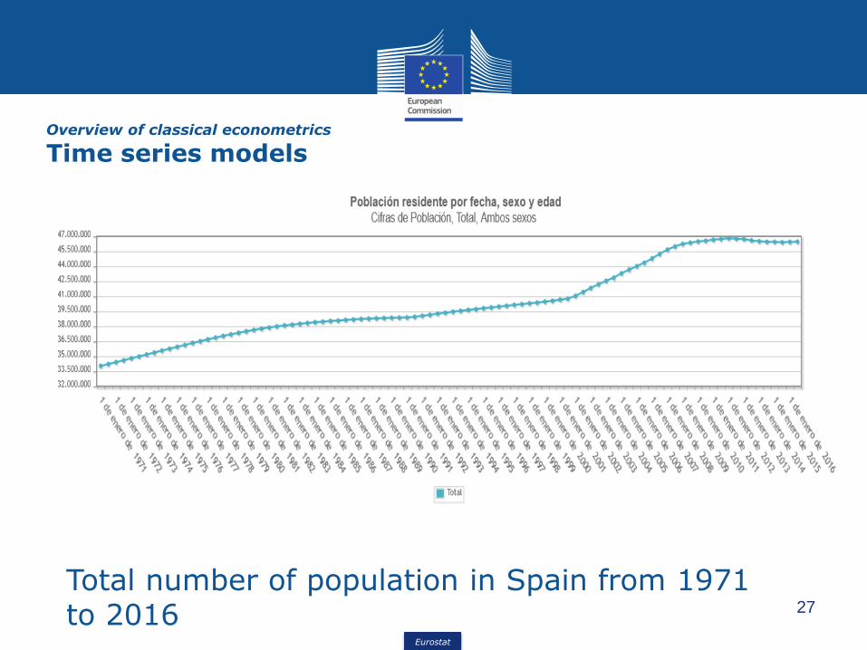
Overview of classical econometrics
Time series models
Total number of population in Spain from 1971 to 2016
Eurostat
28
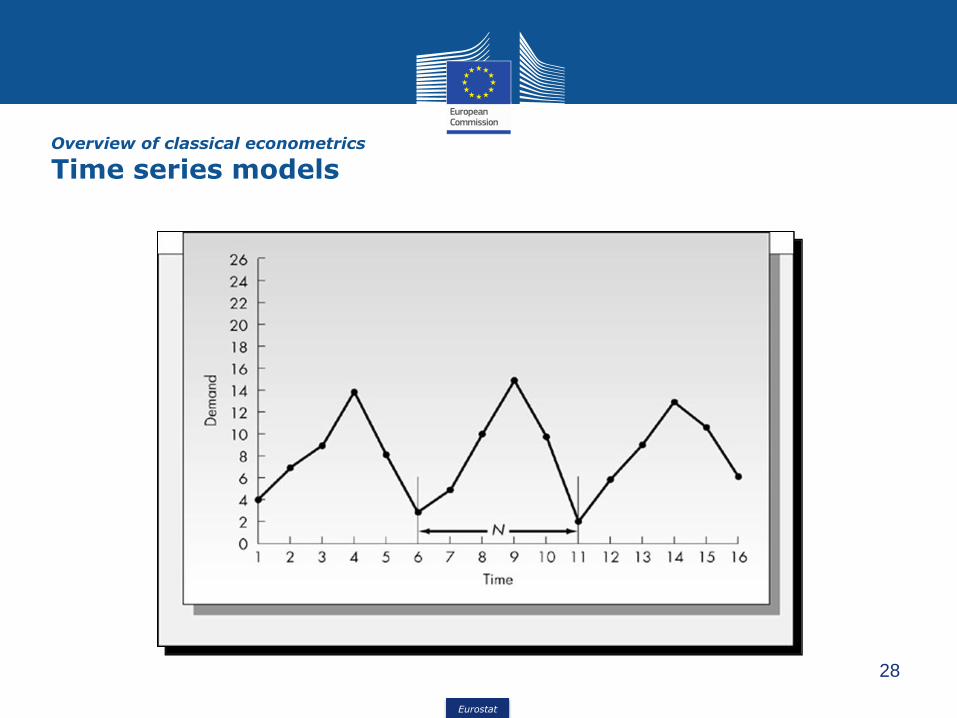
Overview of classical econometrics
Time series models

Eurostat
29
Overview of classical econometrics
Time series models

Eurostat
30
Overview of classical econometrics
Time series models
Univariate Time Series describe the behaviourof a variable in terms of its own past values
𝑌𝑡 = 𝛽0 + 𝛽1𝑌𝑡−1 + 휀𝑡
intercept coefficient
Random error (white noise)
Multivariate Time Series describe the behaviourof a variable in terms of its own past values andthe past values of other variables
𝑌𝑡 = 𝛽0 + 𝛽1𝑌𝑡−1 + 𝛿1𝑋𝑡−1 + 휀𝑡

Eurostat
31
Overview of classical econometrics
Time series models
First order autoregression (AR1)
𝑌𝑡 = 𝛽0 + 𝛽1𝑌𝑡−1 + 휀𝑡
Second order autoregression (AR2)
𝑌𝑡 = 𝛽0 + 𝛽1𝑌𝑡−1 + 𝛽2𝑌𝑡−2휀𝑡
pth order autoregression (ARp)
𝑌𝑡 = 𝛽0 + 𝛽1𝑌𝑡−1 + 𝛽2𝑌𝑡−2 + 𝛽𝑝𝑌𝑡−𝑝 + 휀𝑡
Eurostat
32
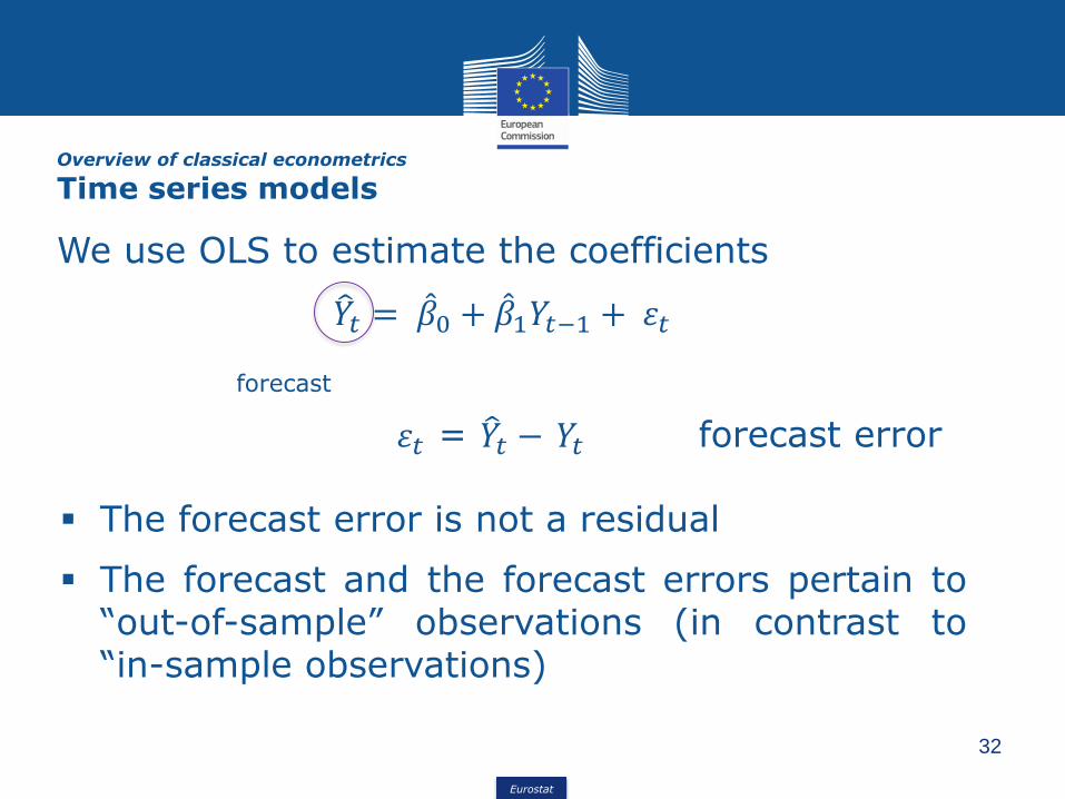
Overview of classical econometrics
Time series models
We use OLS to estimate the coefficients
𝑌𝑡 = መ𝛽0 + መ𝛽1𝑌𝑡−1 + 휀𝑡
휀𝑡 = 𝑌𝑡 − 𝑌𝑡 forecast error
forecast
▪ The forecast error is not a residual
▪ The forecast and the forecast errors pertain to“out-of-sample” observations (in contrast to“in-sample observations)
Eurostat
33
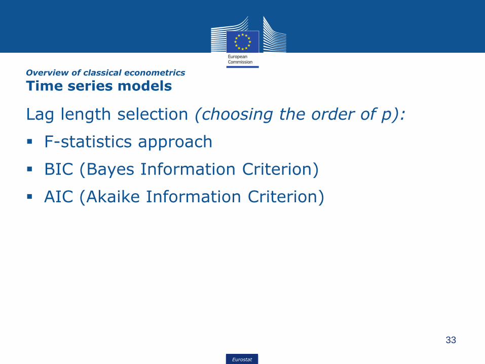
Overview of classical econometrics
Time series models
Lag length selection (choosing the order of p):
▪ F-statistics approach
▪ BIC (Bayes Information Criterion)
▪ AIC (Akaike Information Criterion)
Eurostat
34
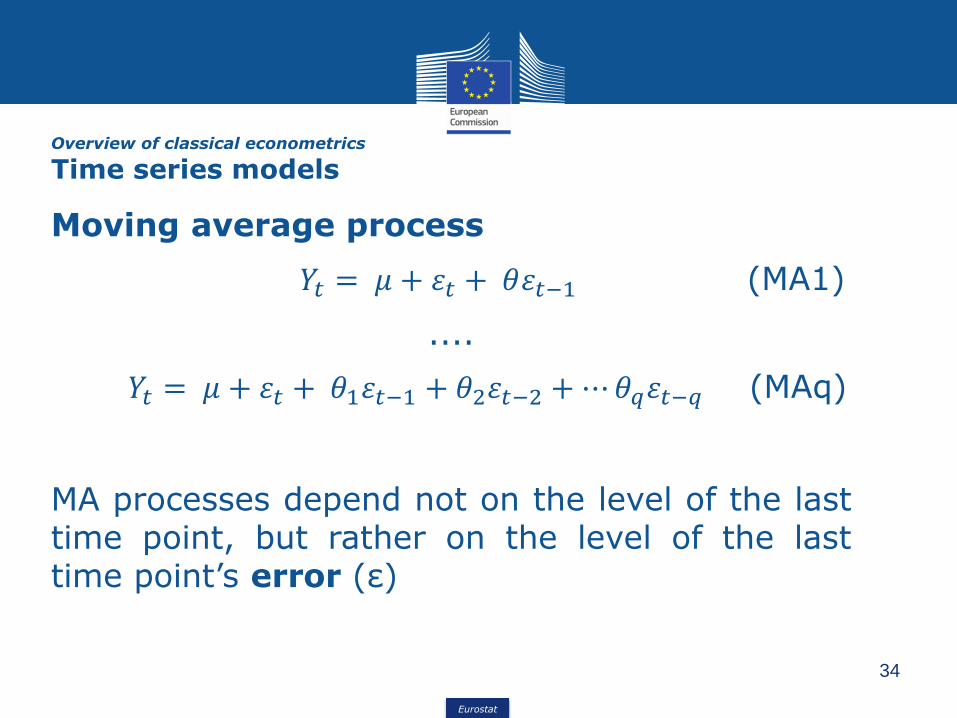
Overview of classical econometrics
Time series models
Moving average process
𝑌𝑡 = 𝜇 + 휀𝑡 + 𝜃휀𝑡−1 (MA1)
....
𝑌𝑡 = 𝜇 + 휀𝑡 + 𝜃1휀𝑡−1 + 𝜃2휀𝑡−2 +⋯𝜃𝑞휀𝑡−𝑞 (MAq)
MA processes depend not on the level of the lasttime point, but rather on the level of the lasttime point’s error (ε)
Eurostat
35
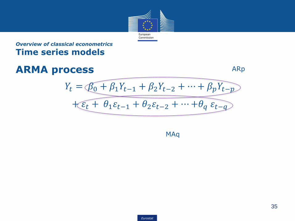
Overview of classical econometrics
Time series models
ARMA process
𝑌𝑡 = 𝛽0 + 𝛽1𝑌𝑡−1 + 𝛽2𝑌𝑡−2 +⋯+ 𝛽𝑝𝑌𝑡−𝑝
+ 휀𝑡 + 𝜃1휀𝑡−1 + 𝜃2휀𝑡−2 +⋯+𝜃𝑞 휀𝑡−𝑞
ARp
MAq
Eurostat
36
Overview of classical econometrics
Time series models
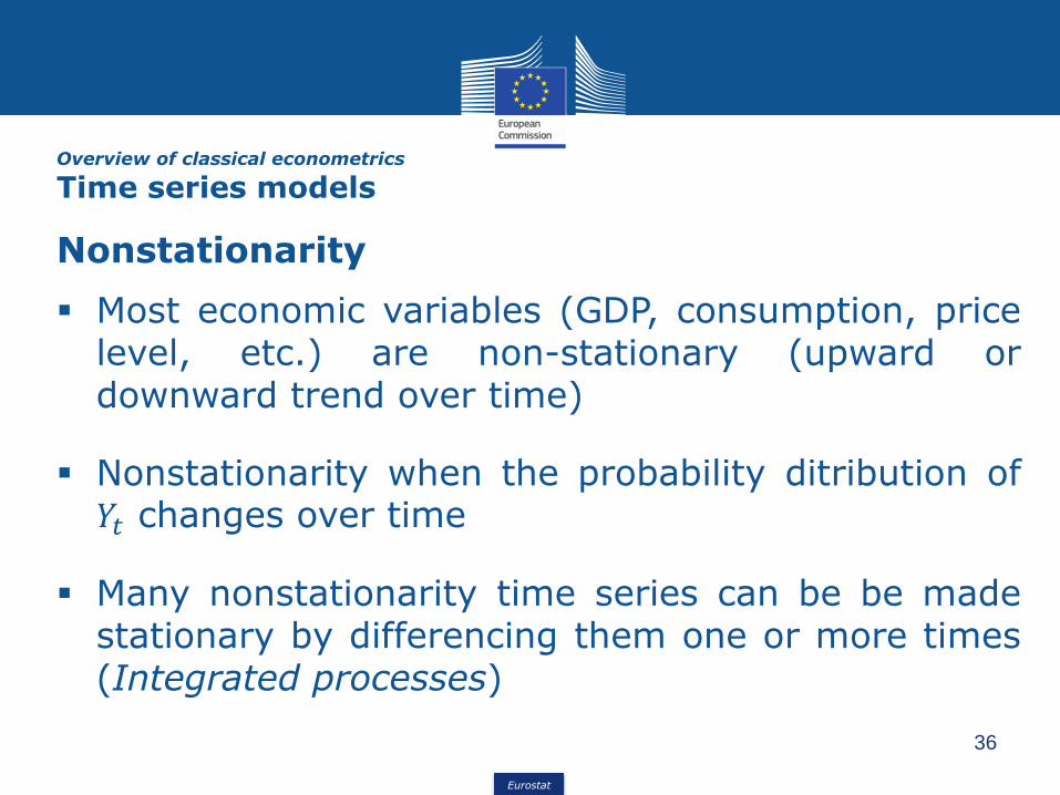
Nonstationarity
▪ Most economic variables (GDP, consumption, pricelevel, etc.) are non-stationary (upward ordownward trend over time)
▪ Nonstationarity when the probability ditribution of𝑌𝑡 changes over time
▪ Many nonstationarity time series can be be madestationary by differencing them one or more times(Integrated processes)
Eurostat
37
Overview of classical econometrics
Time series models
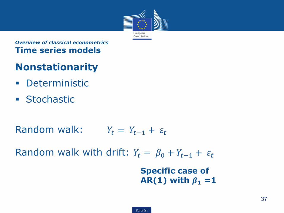
Nonstationarity
▪ Deterministic
▪ Stochastic
Random walk: 𝑌𝑡 = 𝑌𝑡−1 + 휀𝑡
Random walk with drift: 𝑌𝑡 = 𝛽0 + 𝑌𝑡−1 + 휀𝑡
Specific case of AR(1) with 𝜷𝟏 =1

Eurostat
38
Overview of classical econometrics
Time series models
If 𝛽1 = 1 nonstationary time series
If | 𝛽1| <1 stationary time series
𝜷𝟏 = 1 is called Unit root
Eurostat
39
Overview of classical econometrics
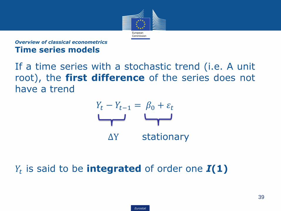
Time series models
If a time series with a stochastic trend (i.e. A unitroot), the first difference of the series does nothave a trend
𝑌𝑡 − 𝑌𝑡−1 = 𝛽0 + 휀𝑡
∆Y stationary
𝑌𝑡 is said to be integrated of order one I(1)

Eurostat
40
Overview of classical econometrics
Time series models
▪ 𝑌𝑡 is said to be integrated of order d I(d) if it
becomes stationary after being first differenced dtimes
▪ Resulting model is ARIMA model
∆dY = 𝛽0 + 𝛽1∆d𝑌𝑡−1 + 𝛽2∆
d𝑌𝑡−2 +⋯+ 𝛽𝑝∆d𝑌𝑡−𝑝
+ 휀𝑡 + 𝜃1휀𝑡−1 + 𝜃2휀𝑡−2 +⋯+𝜃𝑞 휀𝑡−𝑞
Eurostat
41
Overview of classical econometrics
Time series models
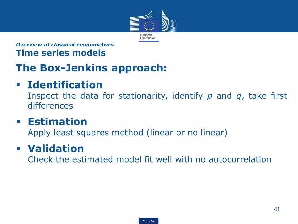
The Box-Jenkins approach:
▪ IdentificationInspect the data for stationarity, identify p and q, take firstdifferences
▪ EstimationApply least squares method (linear or no linear)
▪ ValidationCheck the estimated model fit well with no autocorrelation

Eurostat
4. Econometric methods in Official statistics
Eurostat
43
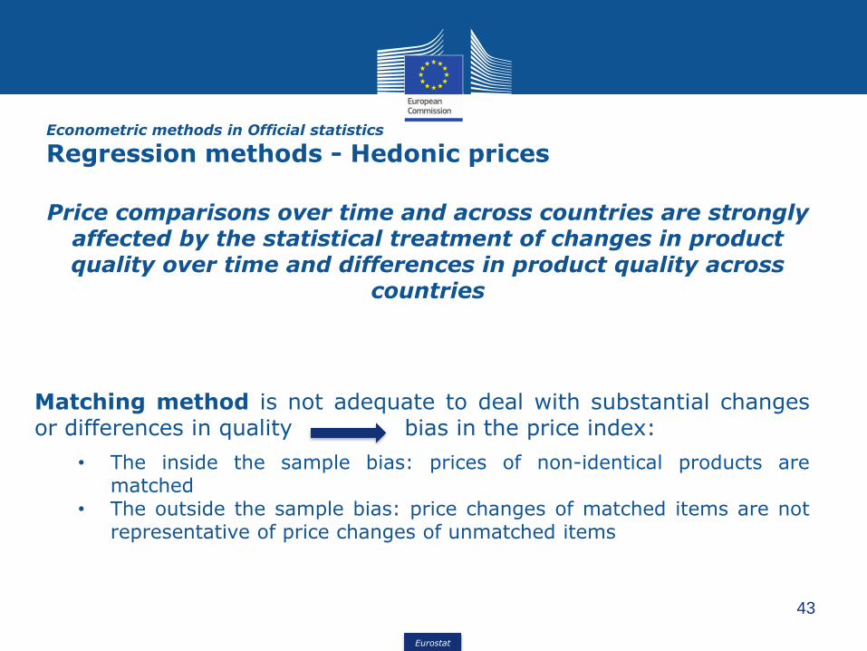
Econometric methods in Official statistics
Regression methods - Hedonic prices
Price comparisons over time and across countries are strongly affected by the statistical treatment of changes in product quality over time and differences in product quality across
countries
Matching method is not adequate to deal with substantial changesor differences in quality bias in the price index:
• The inside the sample bias: prices of non-identical products arematched
• The outside the sample bias: price changes of matched items are notrepresentative of price changes of unmatched items
Eurostat
44
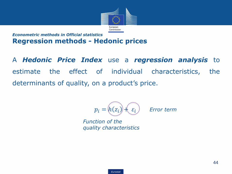
A Hedonic Price Index use a regression analysis to
estimate the effect of individual characteristics, the
determinants of quality, on a product’s price.
𝑝𝑖 = ℎ 𝑧𝑖 + 휀𝑖
Function of the quality characteristics
Error term
Econometric methods in Official statistics
Regression methods - Hedonic prices
Eurostat
45
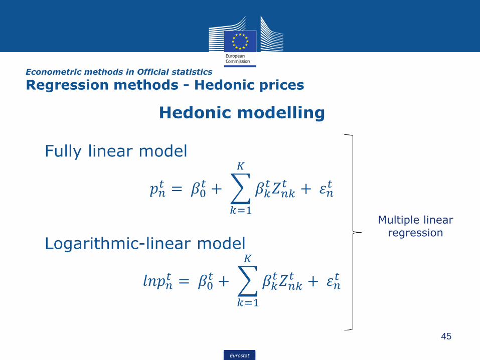
Hedonic modelling
Fully linear model
𝑝𝑛𝑡 = 𝛽0
𝑡 +
𝑘=1
𝐾
𝛽𝑘𝑡𝑍𝑛𝑘
𝑡 + 휀𝑛𝑡
Logarithmic-linear model
𝑙𝑛𝑝𝑛𝑡 = 𝛽0
𝑡 +
𝑘=1
𝐾
𝛽𝑘𝑡𝑍𝑛𝑘
𝑡 + 휀𝑛𝑡
Multiple linear regression
Econometric methods in Official statistics
Regression methods - Hedonic prices

Eurostat
46
Applications
• Housing prices
• ICT- product prices
• Producer prices
Econometric methods in Official statistics
Regression methods - Hedonic prices

Eurostat
47
Advantages
✓ Offer a solution for the quality problem in price indices andinternational comparison, provided sufficient information oncharacteristics can be obtained
✓ It is used to estimate the willing to pay for, or marginalcost of producing, the characteristics, or the underlyingdemand or supply functions of these characteristics andcorresponding consumer of producer surplus
Econometric methods in Official statistics
Regression methods - Hedonic prices

Eurostat
48
Difficulties
✓ Characteristics should represent user value and user cost
✓ Needs large datasets BIG DATA
✓ Excluded variables
✓ Other price determining variables: price mark-ups
✓ New features
✓ Multicollinearity
✓ Small quantities
Econometric methods in Official statistics
Regression methods - Hedonic prices
Eurostat
49
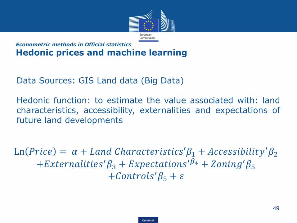
Data Sources: GIS Land data (Big Data)
Hedonic function: to estimate the value associated with: landcharacteristics, accessibility, externalities and expectations offuture land developments
Ln 𝑃𝑟𝑖𝑐𝑒 = 𝛼 + 𝐿𝑎𝑛𝑑 𝐶ℎ𝑎𝑟𝑎𝑐𝑡𝑒𝑟𝑖𝑠𝑡𝑖𝑐𝑠′𝛽1 + 𝐴𝑐𝑐𝑒𝑠𝑠𝑖𝑏𝑖𝑙𝑖𝑡𝑦′𝛽2+𝐸𝑥𝑡𝑒𝑟𝑛𝑎𝑙𝑖𝑡𝑖𝑒𝑠′𝛽3 + 𝐸𝑥𝑝𝑒𝑐𝑡𝑎𝑡𝑖𝑜𝑛𝑠′𝛽4 + 𝑍𝑜𝑛𝑖𝑛𝑔′𝛽5
+𝐶𝑜𝑛𝑡𝑟𝑜𝑙𝑠′𝛽5 + 휀
Econometric methods in Official statistics
Hedonic prices and machine learning

Eurostat
50
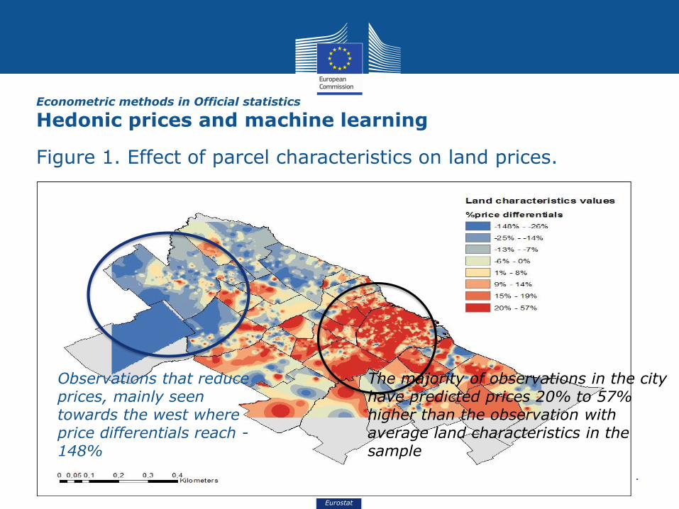
Figure 1. Effect of parcel characteristics on land prices.
The map shows log price differentials generated by different valuesassociated with land characteristics.
i.e. compare the price predicted by the model for each observationcombining all land characteristics and comparing it to the pricepredicted for an ad-hoc observation with mean values for eachexplanatory variable corresponding to this group
Econometric methods in Official statistics
Hedonic prices and machine learning
Eurostat
51
Figure 1. Effect of parcel characteristics on land prices.
The majority of observations in the city have predicted prices 20% to 57% higher than the observation with average land characteristics in the sample
Observations that reduce prices, mainly seen towards the west where price differentials reach -148%
Econometric methods in Official statistics
Hedonic prices and machine learning

Eurostat
52
Figure 2. Accessibility values.
log price differentials generated by different accessibility values
i.e. compare the price predicted by the model for each observationcombining all accessibility variables and comparing it to the pricepredicted for an ad-hoc observation with mean values for eachexplanatory variable corresponding to this group
Econometric methods in Official statistics
Hedonic prices and machine learning

Eurostat
53
Figure 2. Accessibility values.
Proximity to the city center adds value to the land
Econometric methods in Official statistics
Hedonic prices and machine learning

Eurostat
54
Econometric methods in Official statistics
Deseasonalisation
Eurostat
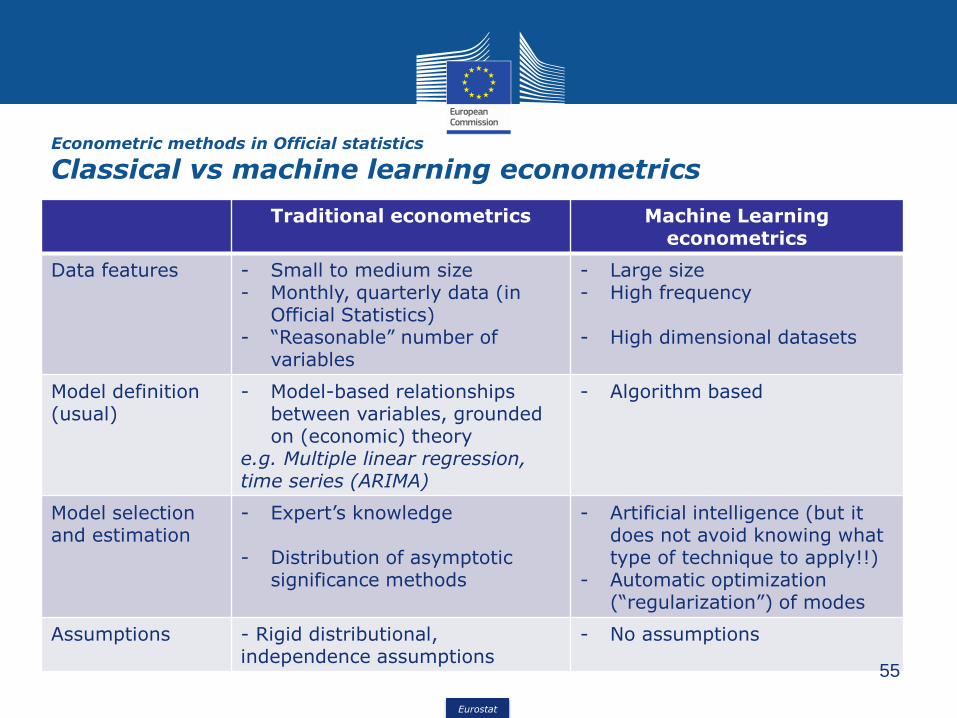
Traditional econometrics Machine Learning econometrics
Data features - Small to medium size- Monthly, quarterly data (in
Official Statistics)- “Reasonable” number of
variables
- Large size- High frequency
- High dimensional datasets
Model definition (usual)
- Model-based relationships between variables, grounded on (economic) theory
e.g. Multiple linear regression, time series (ARIMA)
- Algorithm based
Model selection and estimation
- Expert’s knowledge
- Distribution of asymptotic significance methods
- Artificial intelligence (but it does not avoid knowing what type of technique to apply!!)
- Automatic optimization (“regularization”) of modes
Assumptions - Rigid distributional, independence assumptions
- No assumptions
55
Econometric methods in Official statistics
Classical vs machine learning econometrics

Eurostat
5. Models of inference

Eurostat
• Budget restrictions to carry out traditional surveys
• Increasing concern for response burden
• Increasing non-response
• New sources of available data:
➢ Administrative data
➢ Big Data sources: traffic sensors, M2M transactions, social media, satellite images…
• Development of mathematical-statistical methods and IT tools that allow for other forms of data treatment
57
Models of inference
The context of Official Statistics

Eurostat
▪ The purpose of statistical inference is to obtain informationabout a population (finite or infinite) from a sample fromthis population
▪ Stochastic assumptions about the individual observationsand/or the population are made
▪ Statistical information of interest includes totals, means,proportions, ratios, quantiles, etc. or the probabilitydistribution of a random variable
58
Models of inference
The objectives of statistical inference
Eurostat
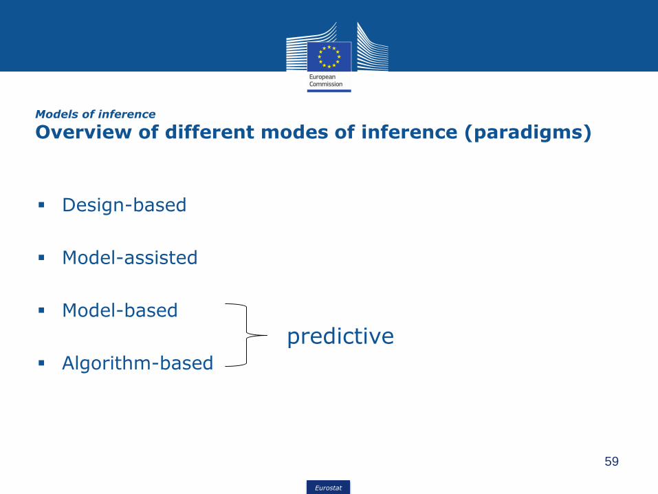
▪ Design-based
▪ Model-assisted
▪ Model-based
▪ Algorithm-based
59
predictive
Models of inference
Overview of different modes of inference (paradigms)
Eurostat
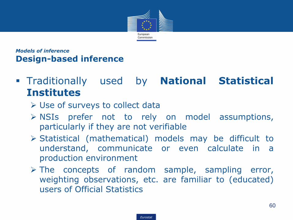
▪ Traditionally used by National StatisticalInstitutes
➢ Use of surveys to collect data
➢ NSIs prefer not to rely on model assumptions,particularly if they are not verifiable
➢ Statistical (mathematical) models may be difficult tounderstand, communicate or even calculate in aproduction environment
➢ The concepts of random sample, sampling error,weighting observations, etc. are familiar to (educated)users of Official Statistics
60
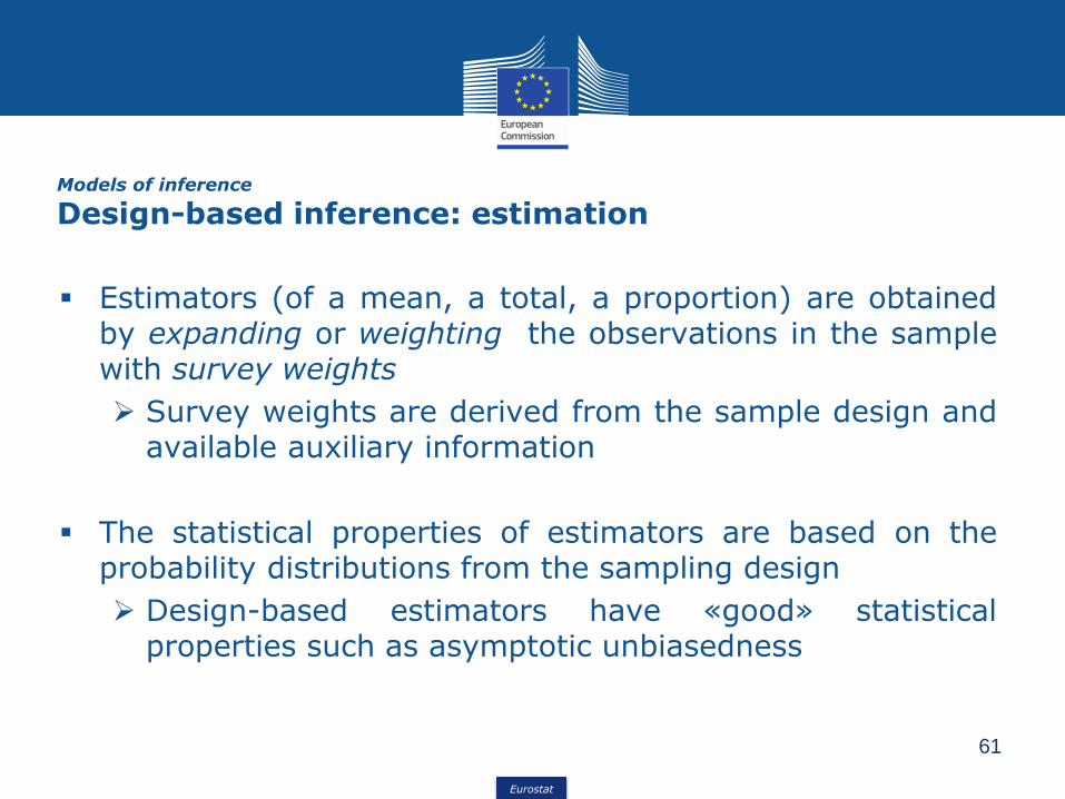
Models of inference
Design-based inference
Eurostat
▪ Estimators (of a mean, a total, a proportion) are obtainedby expanding or weighting the observations in the samplewith survey weights
➢ Survey weights are derived from the sample design andavailable auxiliary information
▪ The statistical properties of estimators are based on theprobability distributions from the sampling design
➢ Design-based estimators have «good» statisticalproperties such as asymptotic unbiasedness
61
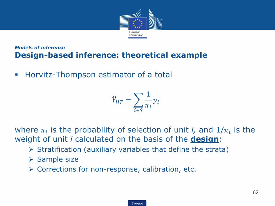
Models of inference
Design-based inference: estimation
Eurostat
▪ Horvitz-Thompson estimator of a total
𝑌𝐻𝑇 =
𝑖∈𝑆
1
𝜋𝑖𝑦𝑖
where 𝜋𝑖 is the probability of selection of unit i, and 1/𝜋𝑖 is the weight of unit i calculated on the basis of the design:
➢ Stratification (auxiliary variables that define the strata)
➢ Sample size
➢ Corrections for non-response, calibration, etc.
62
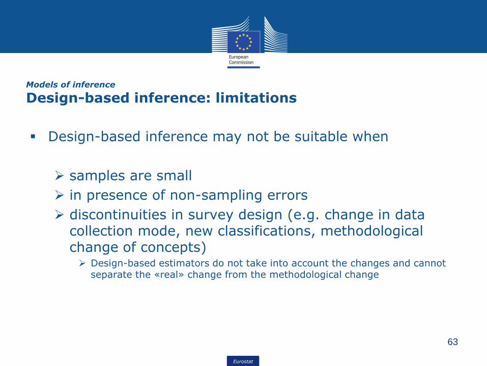
Models of inference
Design-based inference: theoretical example
Eurostat
▪ Design-based inference may not be suitable when
➢ samples are small
➢ in presence of non-sampling errors
➢ discontinuities in survey design (e.g. change in data collection mode, new classifications, methodological change of concepts)➢ Design-based estimators do not take into account the changes and cannot
separate the «real» change from the methodological change
63
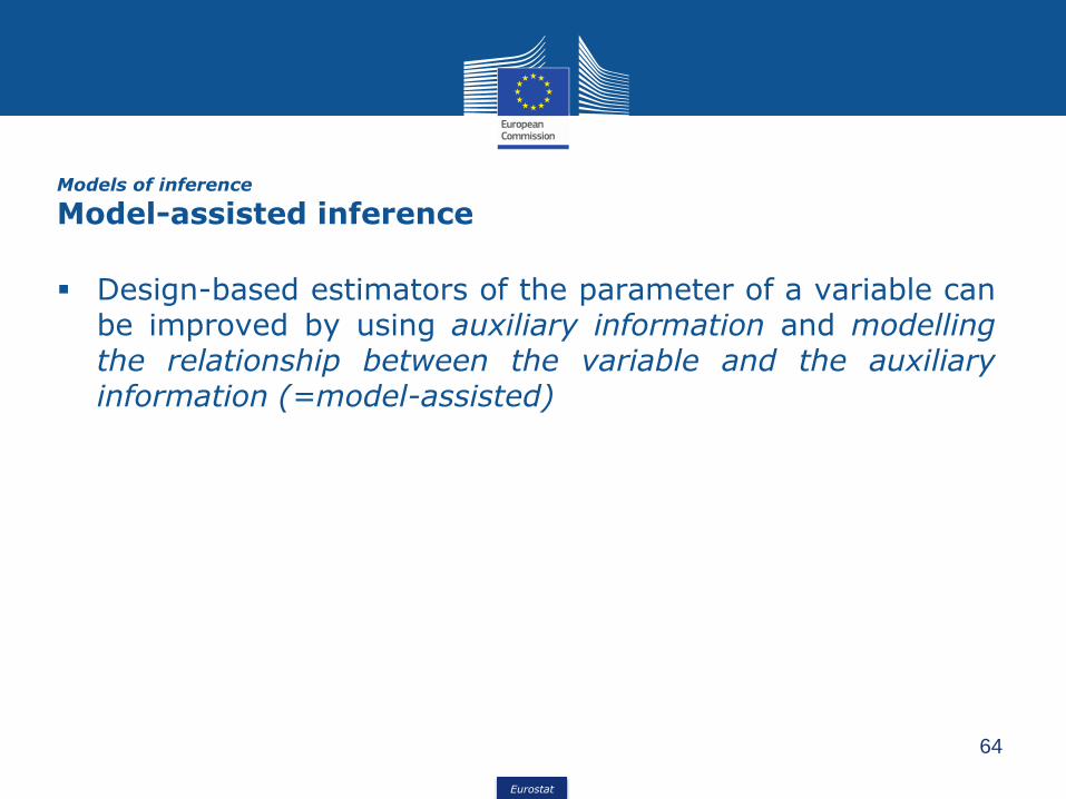
Models of inference
Design-based inference: limitations
Eurostat
▪ Design-based estimators of the parameter of a variable canbe improved by using auxiliary information and modellingthe relationship between the variable and the auxiliaryinformation (=model-assisted)
64
Models of inference
Model-assisted inference
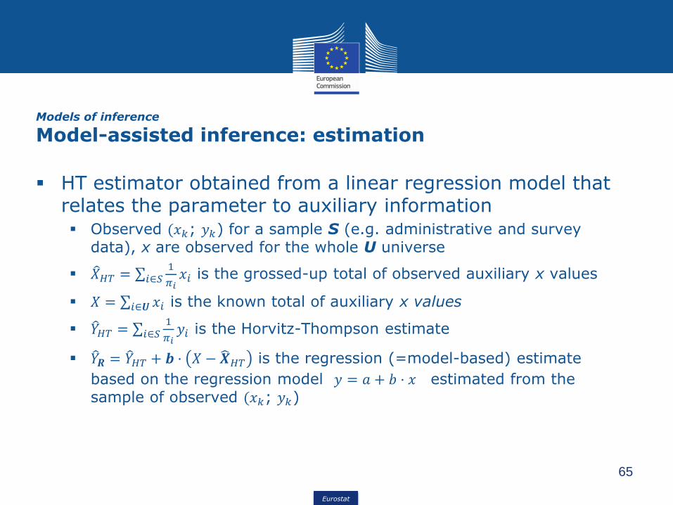
Eurostat
▪ HT estimator obtained from a linear regression model that relates the parameter to auxiliary information▪ Observed (𝑥𝑘; 𝑦𝑘) for a sample S (e.g. administrative and survey
data), x are observed for the whole U universe
▪ 𝑋𝐻𝑇 = σ𝑖∈𝑆1
𝜋𝑖𝑥𝑖 is the grossed-up total of observed auxiliary x values
▪ 𝑋 = σ𝑖∈𝑼 𝑥𝑖 is the known total of auxiliary x values
▪ 𝑌𝐻𝑇 = σ𝑖∈𝑆1
𝜋𝑖𝑦𝑖 is the Horvitz-Thompson estimate
▪ 𝑌𝑹 = 𝑌𝐻𝑇 + 𝒃 · 𝑋 − 𝑿𝐻𝑇 is the regression (=model-based) estimate
based on the regression model 𝑦 = 𝑎 + 𝑏 · 𝑥 estimated from the sample of observed (𝑥𝑘; 𝑦𝑘)
65
Models of inference
Model-assisted inference: estimation
Eurostat
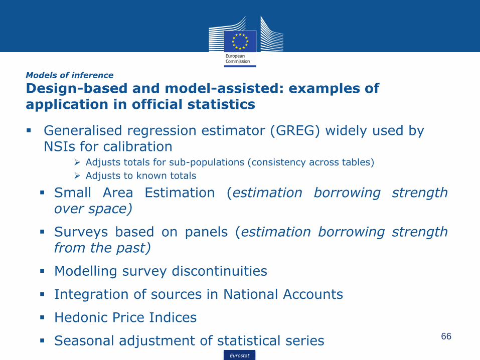
▪ Generalised regression estimator (GREG) widely used by NSIs for calibration
➢ Adjusts totals for sub-populations (consistency across tables)
➢ Adjusts to known totals
▪ Small Area Estimation (estimation borrowing strengthover space)
▪ Surveys based on panels (estimation borrowing strengthfrom the past)
▪ Modelling survey discontinuities
▪ Integration of sources in National Accounts
▪ Hedonic Price Indices
▪ Seasonal adjustment of statistical series 66
Models of inference
Design-based and model-assisted: examples of application in official statistics

Eurostat
• In the algorithmic approach, the equivalent of fitting a model is tuning an algorithm, so that it predicts well
• It is generally impossible to express algorithmic methods analytically in terms of a mathematical expression
• In the algorithmic approach, the data for which both x and y are known is split into two parts• TRAINING SET: part is used to tune the algorithm
• TEST SET: part used to evaluate – or test – the predictive capabilities of the trained algorithm
67
Models of inference
Algorithm-based inference
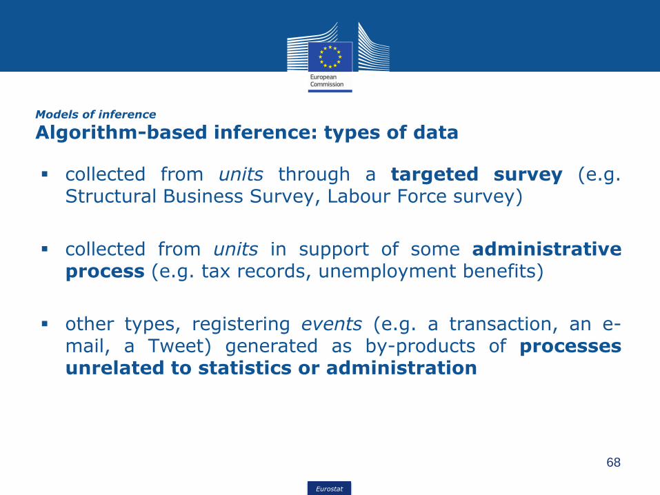
Eurostat
▪ collected from units through a targeted survey (e.g.Structural Business Survey, Labour Force survey)
▪ collected from units in support of some administrativeprocess (e.g. tax records, unemployment benefits)
▪ other types, registering events (e.g. a transaction, an e-mail, a Tweet) generated as by-products of processesunrelated to statistics or administration
68
Models of inference
Algorithm-based inference: types of data
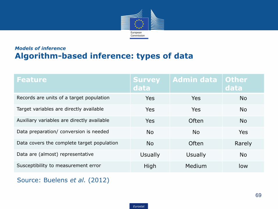
Eurostat
Feature Survey data
Admin data Other data
Records are units of a target population Yes Yes No
Target variables are directly available Yes Yes No
Auxiliary variables are directly available Yes Often No
Data preparation/ conversion is needed No No Yes
Data covers the complete target population No Often Rarely
Data are (almost) representative Usually Usually No
Susceptibility to measurement error High Medium low
69
Source: Buelens et al. (2012)
Models of inference
Algorithm-based inference: types of data
Eurostat
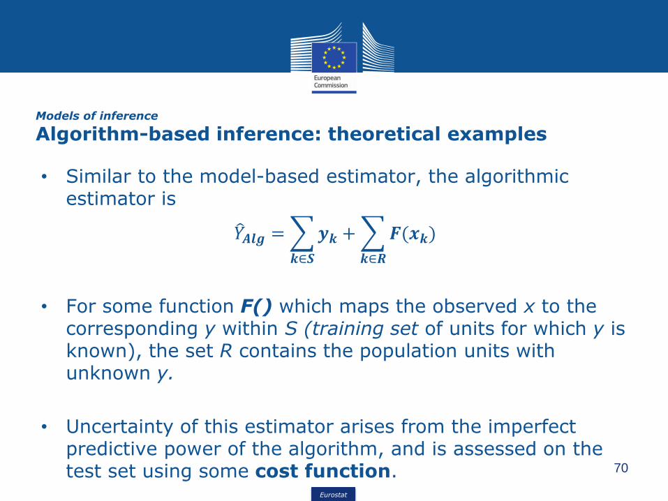
• Similar to the model-based estimator, the algorithmic estimator is
𝑌𝑨𝒍𝒈 =
𝒌∈𝑺
𝒚𝒌 +
𝒌∈𝑹
𝑭(𝒙𝒌)
• For some function F() which maps the observed x to the corresponding y within S (training set of units for which y is known), the set R contains the population units with unknown y.
• Uncertainty of this estimator arises from the imperfect predictive power of the algorithm, and is assessed on the test set using some cost function. 70
Models of inference
Algorithm-based inference: theoretical examples

Eurostat
71
▪ Central Statistics Office of Ireland: automatic codingsystem for Classification of Individual Consumption byPurpose (COICOP) assignment for their Household BudgetSurvey, using previously coded records as training data
▪ Statistics New Zealand: Support Vector Machines (SVM)to improve coding of variables Occupation and Post-schoolQualification, using two disjoint sets of observations, eachof size 10,000, from Census 2013 data for training andtesting (50% correctness).
▪ Statistics Portugal: classification trees (a type of decisiontrees whose response variables are categorical) for errordetection in foreign trade transaction data.
Models of inference
Algorithm-based inference: examples of application in official statistics
Eurostat
72
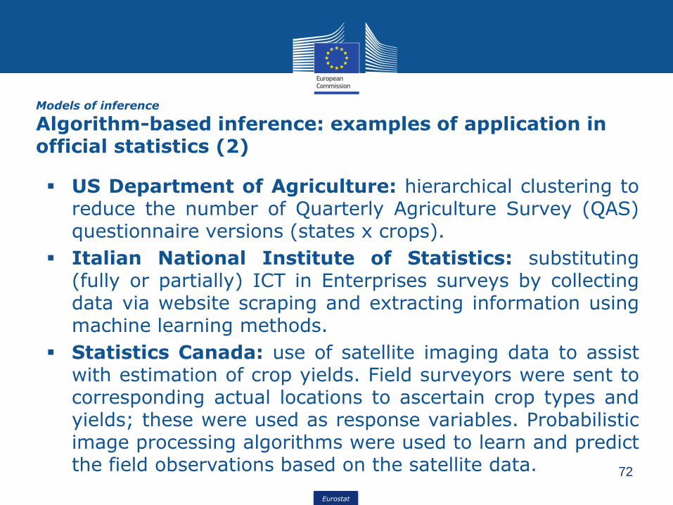
▪ US Department of Agriculture: hierarchical clustering toreduce the number of Quarterly Agriculture Survey (QAS)questionnaire versions (states x crops).
▪ Italian National Institute of Statistics: substituting(fully or partially) ICT in Enterprises surveys by collectingdata via website scraping and extracting information usingmachine learning methods.
▪ Statistics Canada: use of satellite imaging data to assistwith estimation of crop yields. Field surveyors were sent tocorresponding actual locations to ascertain crop types andyields; these were used as response variables. Probabilisticimage processing algorithms were used to learn and predictthe field observations based on the satellite data.
Models of inference
Algorithm-based inference: examples of application in official statistics (2)
Eurostat
▪ J.H. Stock and M.W. Watson (2003). Introduction to econometrics, Addison Wesley
▪ W.H. Green (2003). Econometrics analysis, Prentice Hall
▪ J. van den Brakel and J. Betlehem (2008). Model-based estimation for official statistics. Statistics Netherlands, discussion paper (08002)
▪ K. Chu and Cl. Poirier, Statistics Canada (2015). Machine Learning Documentation Initiative. HIGH-LEVEL GROUP FOR THE MODERNISATION OF STATISTICAL PRODUCTION AND SERVICES, Modernisation Committee on Production and Methods
▪ Buelens, B. H.J. Boonstra, J. van den Brakel, P. Daas (2012). Shifting paradigms in official statistics. Statistics Netherlands, discussion paper (201218)
▪ CROS Portal on MEMOBUST:
▪ Generalised Regression Estimator (Method)
▪ Calibration (Method)
73
References

Eurostat
▪ OECD, Eurostat, ILO, IMF, The World Bank, UNECE (2013). Handbook onResidential Property Price Indices (RPPIs)
▪ Peter Hein van Mulligen (2003). Quality aspects in price indices and international comparisons: Applications of the hedonic method
▪ C. Goytia and G. Dorna (Universidad Torcuato Di Tella)(2016). Big data and a Spatial Hedonic Approach: Addressing the land market information gap and estimating land prices determinants in metropolitan regions from developing countries
74
References