models.plasma.electrodeless lamp
DESCRIPTION
engineeringTRANSCRIPT
Solved with COMSOL Multiphysics 5.0
E l e c t r o d e l e s s L amp
Introduction
This model simulates an electrodeless lamp with argon/mercury chemistry. The low excitation threshold for mercury atoms means that even though the mercury is present in small concentrations, its interaction with electrons determines the overall discharge characteristics. here is strong UV emission from the plasma at 185 nm and 253 nm stemming from spontaneous decay of electronically excited mercury atoms. The UV emission can stimulate phosphors coated on the surface of the bulb resulting in visible light. From an electrical point of view, the lamp can be thought of as a transformer, where the coil acts as the primary and the plasma acts as the secondary. If the efficiency of discharge lamps could be increased by 1%, it would result in a saving of 109 kWh per year worldwide.
Note: This model requires the Plasma Module and the AC/DC Module.
Model Definition
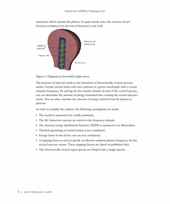
A schematic of the geometry used to solve the problem is given in Figure 1. A sinusoidal current is applied to the copper coil (green) which creates a magnetic field in the ferrite core (gray). When the plasma ignites, a magnetic circuit is created between the ferrite core and the plasma. The free electrons in the plasma bulk are accelerated by the electric field. This leads to creation of new electrons through
1 | E L E C T R O D E L E S S L A M P
Solved with COMSOL Multiphysics 5.0
2 | E L E C
ionization which sustains the plasma. In quasi steady-state, the creation of new electrons is balanced by the loss of electrons to the wall.
Figure 1: Diagram of electrodeless light source.
The presence of mercury leads to the formation of electronically excited mercury atoms. Certain excited states will emit a photon at a given wavelength with a certain emission frequency. By solving for the number density of each of the excited species, you can determine the amount of energy channeled into creating the excited mercury atoms. You can then calculate the amount of energy emitted from the plasma as photons.
In order to simplify the analysis, the following assumptions are made:
• The model is assumed to be axially symmetric.
• The AC induction currents are solved in the frequency domain.
• The electron energy distribution function (EEDF) is assumed to be Maxwellian.
• Thermal quenching of excited atoms is not considered.
• Energy losses in the ferrite core are not considered.
• A trapping factor is used to specify an effective emission photon frequency for the excited mercury atoms. These trapping factors are based on published data.
• The electronically excited argon species are lumped into a single species.
T R O D E L E S S L A M P
Solved with COMSOL Multiphysics 5.0
P L A S M A C H E M I S T R Y
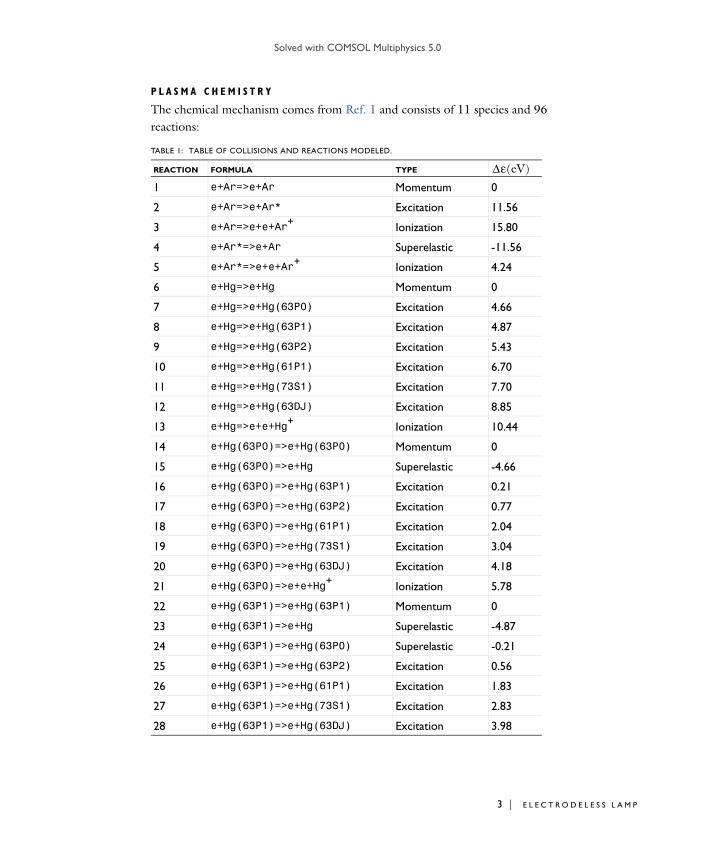
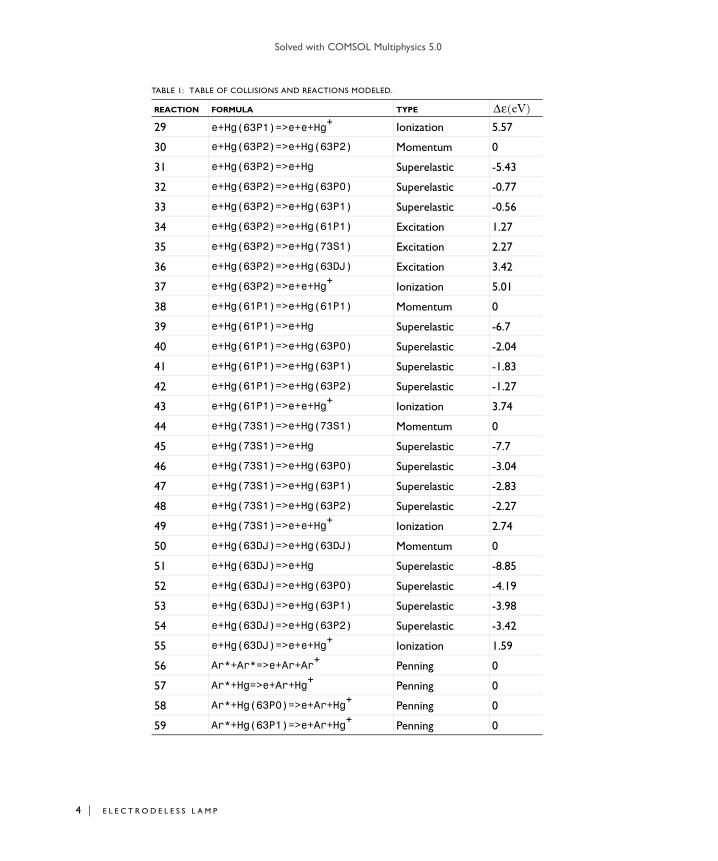
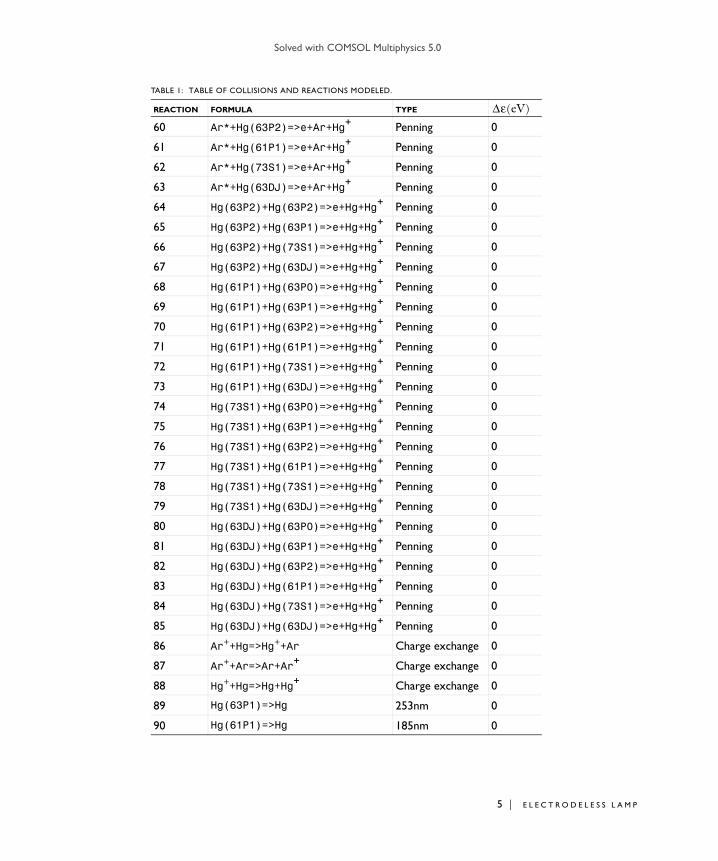
The chemical mechanism comes from Ref. 1 and consists of 11 species and 96 reactions:
TABLE 1: TABLE OF COLLISIONS AND REACTIONS MODELED.
REACTION FORMULA TYPE
1 e+Ar=>e+Ar Momentum 0
2 e+Ar=>e+Ar* Excitation 11.56
3 e+Ar=>e+e+Ar+ Ionization 15.80
4 e+Ar*=>e+Ar Superelastic -11.56
5 e+Ar*=>e+e+Ar+ Ionization 4.24
6 e+Hg=>e+Hg Momentum 0
7 e+Hg=>e+Hg(63P0) Excitation 4.66
8 e+Hg=>e+Hg(63P1) Excitation 4.87
9 e+Hg=>e+Hg(63P2) Excitation 5.43
10 e+Hg=>e+Hg(61P1) Excitation 6.70
11 e+Hg=>e+Hg(73S1) Excitation 7.70
12 e+Hg=>e+Hg(63DJ) Excitation 8.85
13 e+Hg=>e+e+Hg+ Ionization 10.44
14 e+Hg(63P0)=>e+Hg(63P0) Momentum 0
15 e+Hg(63P0)=>e+Hg Superelastic -4.66
16 e+Hg(63P0)=>e+Hg(63P1) Excitation 0.21
17 e+Hg(63P0)=>e+Hg(63P2) Excitation 0.77
18 e+Hg(63P0)=>e+Hg(61P1) Excitation 2.04
19 e+Hg(63P0)=>e+Hg(73S1) Excitation 3.04
20 e+Hg(63P0)=>e+Hg(63DJ) Excitation 4.18
21 e+Hg(63P0)=>e+e+Hg+ Ionization 5.78
22 e+Hg(63P1)=>e+Hg(63P1) Momentum 0
23 e+Hg(63P1)=>e+Hg Superelastic -4.87
24 e+Hg(63P1)=>e+Hg(63P0) Superelastic -0.21
25 e+Hg(63P1)=>e+Hg(63P2) Excitation 0.56
26 e+Hg(63P1)=>e+Hg(61P1) Excitation 1.83
27 e+Hg(63P1)=>e+Hg(73S1) Excitation 2.83
28 e+Hg(63P1)=>e+Hg(63DJ) Excitation 3.98
Δε(eV)
3 | E L E C T R O D E L E S S L A M P
Solved with COMSOL Multiphysics 5.0
4 | E L E C
29 e+Hg(63P1)=>e+e+Hg+ Ionization 5.57
30 e+Hg(63P2)=>e+Hg(63P2) Momentum 0
31 e+Hg(63P2)=>e+Hg Superelastic -5.43
32 e+Hg(63P2)=>e+Hg(63P0) Superelastic -0.77
33 e+Hg(63P2)=>e+Hg(63P1) Superelastic -0.56
34 e+Hg(63P2)=>e+Hg(61P1) Excitation 1.27
35 e+Hg(63P2)=>e+Hg(73S1) Excitation 2.27
36 e+Hg(63P2)=>e+Hg(63DJ) Excitation 3.42
37 e+Hg(63P2)=>e+e+Hg+ Ionization 5.01
38 e+Hg(61P1)=>e+Hg(61P1) Momentum 0
39 e+Hg(61P1)=>e+Hg Superelastic -6.7
40 e+Hg(61P1)=>e+Hg(63P0) Superelastic -2.04
41 e+Hg(61P1)=>e+Hg(63P1) Superelastic -1.83
42 e+Hg(61P1)=>e+Hg(63P2) Superelastic -1.27
43 e+Hg(61P1)=>e+e+Hg+ Ionization 3.74
44 e+Hg(73S1)=>e+Hg(73S1) Momentum 0
45 e+Hg(73S1)=>e+Hg Superelastic -7.7
46 e+Hg(73S1)=>e+Hg(63P0) Superelastic -3.04
47 e+Hg(73S1)=>e+Hg(63P1) Superelastic -2.83
48 e+Hg(73S1)=>e+Hg(63P2) Superelastic -2.27
49 e+Hg(73S1)=>e+e+Hg+ Ionization 2.74
50 e+Hg(63DJ)=>e+Hg(63DJ) Momentum 0
51 e+Hg(63DJ)=>e+Hg Superelastic -8.85
52 e+Hg(63DJ)=>e+Hg(63P0) Superelastic -4.19
53 e+Hg(63DJ)=>e+Hg(63P1) Superelastic -3.98
54 e+Hg(63DJ)=>e+Hg(63P2) Superelastic -3.42
55 e+Hg(63DJ)=>e+e+Hg+ Ionization 1.59
56 Ar*+Ar*=>e+Ar+Ar+ Penning 0
57 Ar*+Hg=>e+Ar+Hg+ Penning 0
58 Ar*+Hg(63P0)=>e+Ar+Hg+ Penning 0
59 Ar*+Hg(63P1)=>e+Ar+Hg+ Penning 0
TABLE 1: TABLE OF COLLISIONS AND REACTIONS MODELED.
REACTION FORMULA TYPE Δε(eV)
T R O D E L E S S L A M P
Solved with COMSOL Multiphysics 5.0
60 Ar*+Hg(63P2)=>e+Ar+Hg+ Penning 0
61 Ar*+Hg(61P1)=>e+Ar+Hg+ Penning 0
62 Ar*+Hg(73S1)=>e+Ar+Hg+ Penning 0
63 Ar*+Hg(63DJ)=>e+Ar+Hg+ Penning 0
64 Hg(63P2)+Hg(63P2)=>e+Hg+Hg+ Penning 0
65 Hg(63P2)+Hg(63P1)=>e+Hg+Hg+ Penning 0
66 Hg(63P2)+Hg(73S1)=>e+Hg+Hg+ Penning 0
67 Hg(63P2)+Hg(63DJ)=>e+Hg+Hg+ Penning 0
68 Hg(61P1)+Hg(63P0)=>e+Hg+Hg+ Penning 0
69 Hg(61P1)+Hg(63P1)=>e+Hg+Hg+ Penning 0
70 Hg(61P1)+Hg(63P2)=>e+Hg+Hg+ Penning 0
71 Hg(61P1)+Hg(61P1)=>e+Hg+Hg+ Penning 0
72 Hg(61P1)+Hg(73S1)=>e+Hg+Hg+ Penning 0
73 Hg(61P1)+Hg(63DJ)=>e+Hg+Hg+ Penning 0
74 Hg(73S1)+Hg(63P0)=>e+Hg+Hg+ Penning 0
75 Hg(73S1)+Hg(63P1)=>e+Hg+Hg+ Penning 0
76 Hg(73S1)+Hg(63P2)=>e+Hg+Hg+ Penning 0
77 Hg(73S1)+Hg(61P1)=>e+Hg+Hg+ Penning 0
78 Hg(73S1)+Hg(73S1)=>e+Hg+Hg+ Penning 0
79 Hg(73S1)+Hg(63DJ)=>e+Hg+Hg+ Penning 0
80 Hg(63DJ)+Hg(63P0)=>e+Hg+Hg+ Penning 0
81 Hg(63DJ)+Hg(63P1)=>e+Hg+Hg+ Penning 0
82 Hg(63DJ)+Hg(63P2)=>e+Hg+Hg+ Penning 0
83 Hg(63DJ)+Hg(61P1)=>e+Hg+Hg+ Penning 0
84 Hg(63DJ)+Hg(73S1)=>e+Hg+Hg+ Penning 0
85 Hg(63DJ)+Hg(63DJ)=>e+Hg+Hg+ Penning 0
86 Ar++Hg=>Hg++Ar Charge exchange 0
87 Ar++Ar=>Ar+Ar+ Charge exchange 0
88 Hg++Hg=>Hg+Hg+ Charge exchange 0
89 Hg(63P1)=>Hg 253nm 0
90 Hg(61P1)=>Hg 185nm 0
TABLE 1: TABLE OF COLLISIONS AND REACTIONS MODELED.
REACTION FORMULA TYPE Δε(eV)
5 | E L E C T R O D E L E S S L A M P
Solved with COMSOL Multiphysics 5.0
6 | E L E C
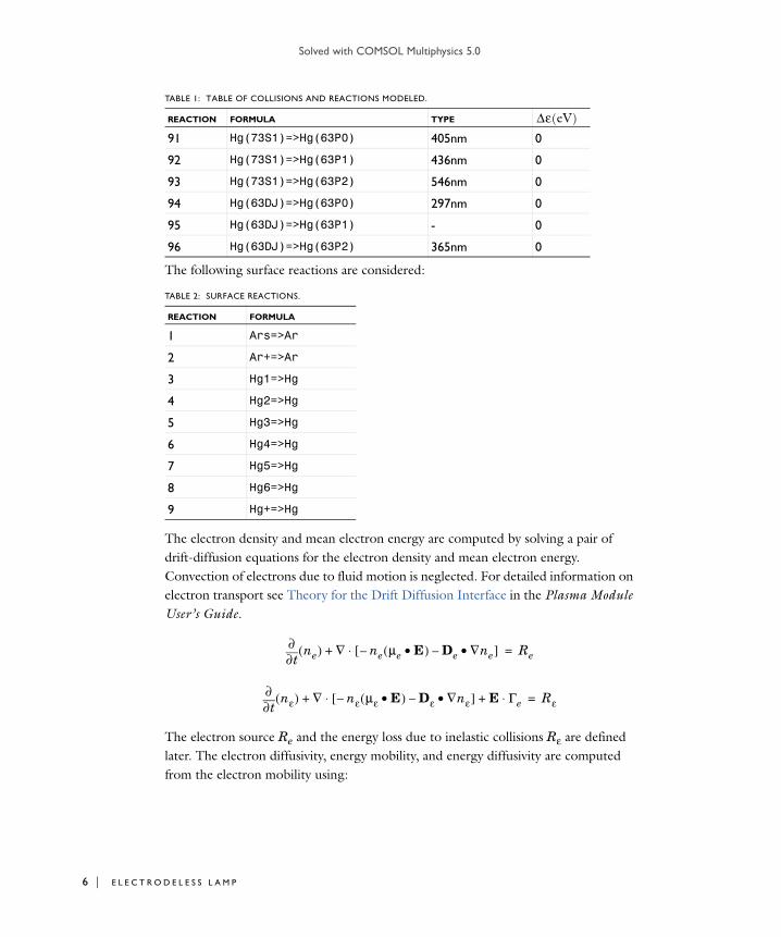
The following surface reactions are considered:
The electron density and mean electron energy are computed by solving a pair of drift-diffusion equations for the electron density and mean electron energy. Convection of electrons due to fluid motion is neglected. For detailed information on electron transport see Theory for the Drift Diffusion Interface in the Plasma Module User’s Guide.
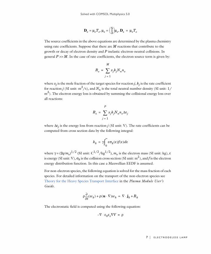
The electron source Re and the energy loss due to inelastic collisions Rε are defined later. The electron diffusivity, energy mobility, and energy diffusivity are computed from the electron mobility using:
91 Hg(73S1)=>Hg(63P0) 405nm 0
92 Hg(73S1)=>Hg(63P1) 436nm 0
93 Hg(73S1)=>Hg(63P2) 546nm 0
94 Hg(63DJ)=>Hg(63P0) 297nm 0
95 Hg(63DJ)=>Hg(63P1) - 0
96 Hg(63DJ)=>Hg(63P2) 365nm 0
TABLE 2: SURFACE REACTIONS.
REACTION FORMULA
1 Ars=>Ar
2 Ar+=>Ar
3 Hg1=>Hg
4 Hg2=>Hg
5 Hg3=>Hg
6 Hg4=>Hg
7 Hg5=>Hg
8 Hg6=>Hg
9 Hg+=>Hg
TABLE 1: TABLE OF COLLISIONS AND REACTIONS MODELED.
REACTION FORMULA TYPE Δε(eV)
t∂∂ ne( ) ∇ ne μe E•( )– De ∇ne•–[ ]⋅+ Re=
t∂∂ nε( ) ∇ nε με E•( )– Dε ∇nε•–[ ] E Γe⋅+⋅+ Rε=
T R O D E L E S S L A M P
Solved with COMSOL Multiphysics 5.0
The source coefficients in the above equations are determined by the plasma chemistry using rate coefficients. Suppose that there are M reactions that contribute to the growth or decay of electron density and P inelastic electron-neutral collisions. In general P >> M. In the case of rate coefficients, the electron source term is given by:
where xj is the mole fraction of the target species for reaction j, kj is the rate coefficient for reaction j (SI unit: m3/s), and Nn is the total neutral number density (SI unit: 1/m3). The electron energy loss is obtained by summing the collisional energy loss over all reactions:
where Δεj is the energy loss from reaction j (SI unit: V). The rate coefficients can be computed from cross section data by the following integral:
where γ = (2q/me)1/2 (SI unit: C1/2/kg1/2), me is the electron mass (SI unit: kg), ε
is energy (SI unit: V), σk is the collision cross section (SI unit: m2), and f is the electron energy distribution function. In this case a Maxwellian EEDF is assumed.
For non-electron species, the following equation is solved for the mass fraction of each species. For detailed information on the transport of the non-electron species see Theory for the Heavy Species Transport Interface in the Plasma Module User’s Guide.
The electrostatic field is computed using the following equation:
De μeTe= με, 53--- μe= Dε, μεTe=
Re xjkjNnne
j 1=
M
=
Rε xjkjNnneΔεj
j 1=
P
=
kk γ εσk ε( )f ε( ) εd0
∞
=
ρt∂
∂ wk( ) ρ u ∇⋅( )wk+ ∇ jk⋅ Rk+=
∇– ε0εr V∇⋅ ρ=
7 | E L E C T R O D E L E S S L A M P
Solved with COMSOL Multiphysics 5.0
8 | E L E C
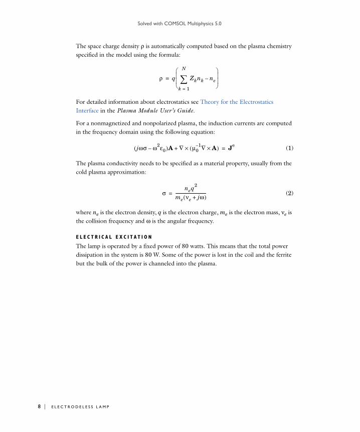
The space charge density ρ is automatically computed based on the plasma chemistry specified in the model using the formula:
For detailed information about electrostatics see Theory for the Electrostatics Interface in the Plasma Module User’s Guide.
For a nonmagnetized and nonpolarized plasma, the induction currents are computed in the frequency domain using the following equation:
(1)
The plasma conductivity needs to be specified as a material property, usually from the cold plasma approximation:
(2)
where ne is the electron density, q is the electron charge, me is the electron mass, νe is the collision frequency and ω is the angular frequency.
E L E C T R I C A L E X C I T A T I O N
The lamp is operated by a fixed power of 80 watts. This means that the total power dissipation in the system is 80 W. Some of the power is lost in the coil and the ferrite but the bulk of the power is channeled into the plasma.
ρ q Zknk
k 1=
N
ne–
=
jωσ ω2ε0–( )A ∇ μ01– ∇ A×( )×+ Je
=
σneq2
me νe jω+( )-------------------------------=
T R O D E L E S S L A M P
Solved with COMSOL Multiphysics 5.0
Results and Discussion
The results are presented below.
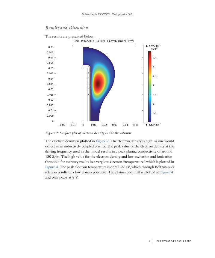
Figure 2: Surface plot of electron density inside the column.
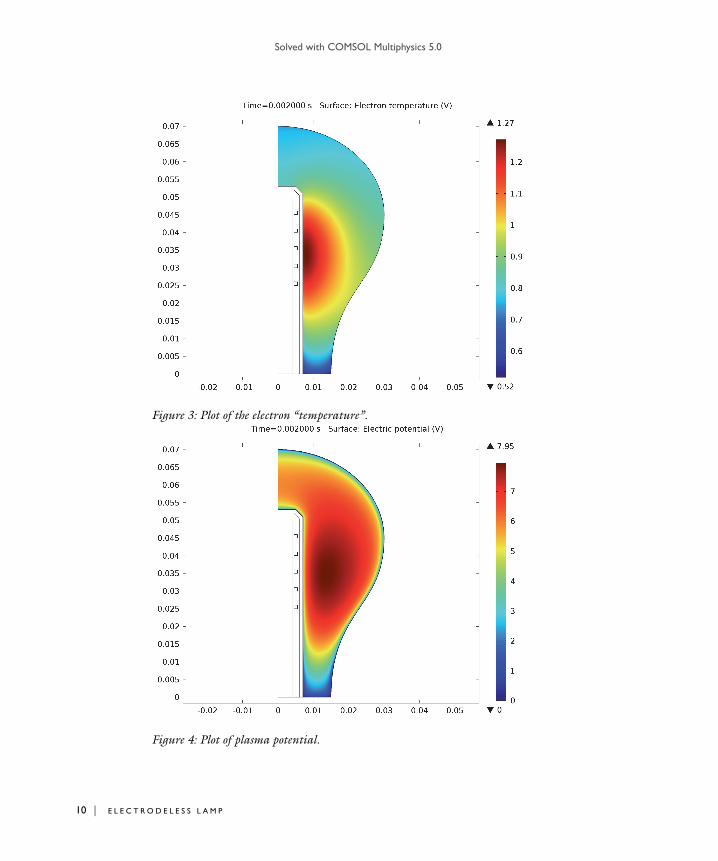
The electron density is plotted in Figure 2. The electron density is high, as one would expect in an inductively coupled plasma. The peak value of the electron density at the driving frequency used in the model results in a peak plasma conductivity of around 180 S/m. The high value for the electron density and low excitation and ionization threshold for mercury results in a very low electron “temperature” which is plotted in Figure 3. The peak electron temperature is only 1.27 eV, which through Boltzmann’s relation results in a low plasma potential. The plasma potential is plotted in Figure 4 and only peaks at 8 V.
9 | E L E C T R O D E L E S S L A M P
Solved with COMSOL Multiphysics 5.0
10 | E L E
Figure 3: Plot of the electron “temperature”.
Figure 4: Plot of plasma potential.
C T R O D E L E S S L A M P
Solved with COMSOL Multiphysics 5.0
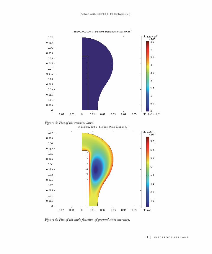
Figure 5: Plot of the resistive losses.
Figure 6: Plot of the mole fraction of ground state mercury.
11 | E L E C T R O D E L E S S L A M P
Solved with COMSOL Multiphysics 5.0
12 | E L E
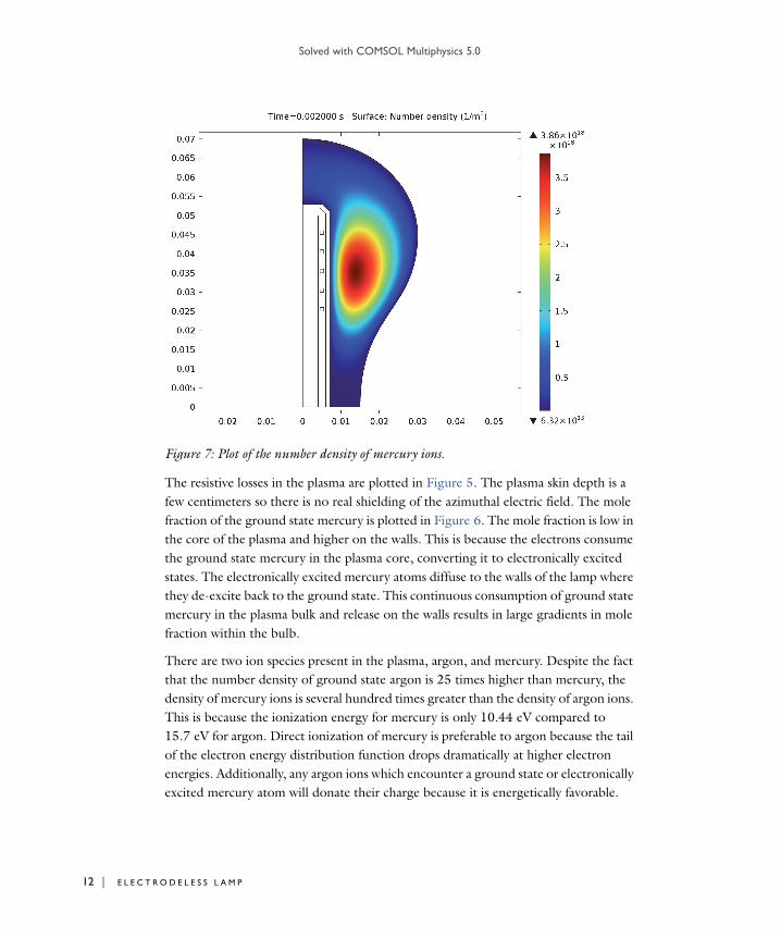
Figure 7: Plot of the number density of mercury ions.
The resistive losses in the plasma are plotted in Figure 5. The plasma skin depth is a few centimeters so there is no real shielding of the azimuthal electric field. The mole fraction of the ground state mercury is plotted in Figure 6. The mole fraction is low in the core of the plasma and higher on the walls. This is because the electrons consume the ground state mercury in the plasma core, converting it to electronically excited states. The electronically excited mercury atoms diffuse to the walls of the lamp where they de-excite back to the ground state. This continuous consumption of ground state mercury in the plasma bulk and release on the walls results in large gradients in mole fraction within the bulb.
There are two ion species present in the plasma, argon, and mercury. Despite the fact that the number density of ground state argon is 25 times higher than mercury, the density of mercury ions is several hundred times greater than the density of argon ions. This is because the ionization energy for mercury is only 10.44 eV compared to 15.7 eV for argon. Direct ionization of mercury is preferable to argon because the tail of the electron energy distribution function drops dramatically at higher electron energies. Additionally, any argon ions which encounter a ground state or electronically excited mercury atom will donate their charge because it is energetically favorable.
C T R O D E L E S S L A M P
Solved with COMSOL Multiphysics 5.0
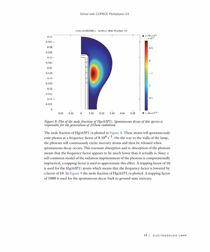
Figure 8: Plot of the mole fraction of Hg(63P1). Spontaneous decay of this species is responsible for the generation of 253nm radiation.
The mole fraction of Hg(63P1) is plotted in Figure 8. These atoms will spontaneously emit photos at a frequency factor of 8·106 s−1. On the way to the walls of the lamp, the photons will continuously excite mercury atoms and then be released when spontaneous decay occurs. This resonant absorption and re-absorption of the photons means that the frequency factor appears to be much lower than it actually is. Since a self consistent model of the radiation imprisonment of the photons is computationally impractical, a trapping factor is used to approximate this effect. A trapping factor of 10 is used for the Hg(63P1) atoms which means that the frequency factor is lowered by a factor of 10. In Figure 9 the mole fraction of Hg(61P1) is plotted. A trapping factor of 1000 is used for the spontaneous decay back to ground state mercury.
13 | E L E C T R O D E L E S S L A M P

Solved with COMSOL Multiphysics 5.0
14 | E L E
Figure 9: Plot of the mole fraction of Hg(61P1). Spontaneous decay of this species is responsible for the generation of 185nm radiation.
Reference
1. K. Rajaraman, Radiation Transport in Low Pressure Plasmas: Lighting and Semiconductor Etching Plasmas, Ph.D. thesis, Depart. of Physics, University of Illinois, 2005.
Model Library path: Plasma_Module/Inductively_Coupled_Plasmas/electrodeless_lamp
Modeling Instructions
From the File menu, choose New.
N E W
1 In the New window, click Model Wizard.
C T R O D E L E S S L A M P
Solved with COMSOL Multiphysics 5.0
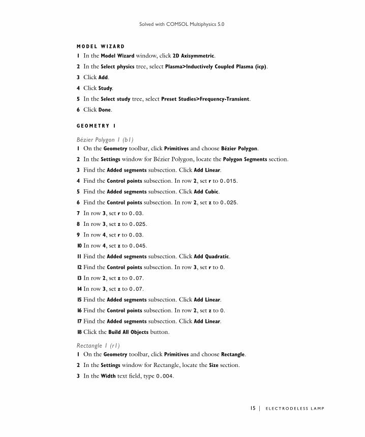
M O D E L W I Z A R D
1 In the Model Wizard window, click 2D Axisymmetric.
2 In the Select physics tree, select Plasma>Inductively Coupled Plasma (icp).
3 Click Add.
4 Click Study.
5 In the Select study tree, select Preset Studies>Frequency-Transient.
6 Click Done.
G E O M E T R Y 1
Bézier Polygon 1 (b1)1 On the Geometry toolbar, click Primitives and choose Bézier Polygon.
2 In the Settings window for Bézier Polygon, locate the Polygon Segments section.
3 Find the Added segments subsection. Click Add Linear.
4 Find the Control points subsection. In row 2, set r to 0.015.
5 Find the Added segments subsection. Click Add Cubic.
6 Find the Control points subsection. In row 2, set z to 0.025.
7 In row 3, set r to 0.03.
8 In row 3, set z to 0.025.
9 In row 4, set r to 0.03.
10 In row 4, set z to 0.045.
11 Find the Added segments subsection. Click Add Quadratic.
12 Find the Control points subsection. In row 3, set r to 0.
13 In row 2, set z to 0.07.
14 In row 3, set z to 0.07.
15 Find the Added segments subsection. Click Add Linear.
16 Find the Control points subsection. In row 2, set z to 0.
17 Find the Added segments subsection. Click Add Linear.
18 Click the Build All Objects button.
Rectangle 1 (r1)1 On the Geometry toolbar, click Primitives and choose Rectangle.
2 In the Settings window for Rectangle, locate the Size section.
3 In the Width text field, type 0.004.
15 | E L E C T R O D E L E S S L A M P
Solved with COMSOL Multiphysics 5.0
16 | E L E
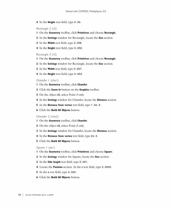
4 In the Height text field, type 0.05.
Rectangle 2 (r2)1 On the Geometry toolbar, click Primitives and choose Rectangle.
2 In the Settings window for Rectangle, locate the Size section.
3 In the Width text field, type 0.006.
4 In the Height text field, type 0.052.
Rectangle 3 (r3)1 On the Geometry toolbar, click Primitives and choose Rectangle.
2 In the Settings window for Rectangle, locate the Size section.
3 In the Width text field, type 0.007.
4 In the Height text field, type 0.053.
Chamfer 1 (cha1)1 On the Geometry toolbar, click Chamfer.
2 Click the Zoom In button on the Graphics toolbar.
3 On the object r2, select Point 3 only.
4 In the Settings window for Chamfer, locate the Distance section.
5 In the Distance from vertex text field, type 1.5e-3.
6 Click the Build All Objects button.
Chamfer 2 (cha2)1 On the Geometry toolbar, click Chamfer.
2 On the object r3, select Point 3 only.
3 In the Settings window for Chamfer, locate the Distance section.
4 In the Distance from vertex text field, type 2e-3.
5 Click the Build All Objects button.
Square 1 (sq1)1 On the Geometry toolbar, click Primitives and choose Square.
2 In the Settings window for Square, locate the Size section.
3 In the Side length text field, type 0.001.
4 Locate the Position section. In the r text field, type 0.0045.
5 In the z text field, type 0.025.
6 Click the Build All Objects button.
C T R O D E L E S S L A M P
Solved with COMSOL Multiphysics 5.0
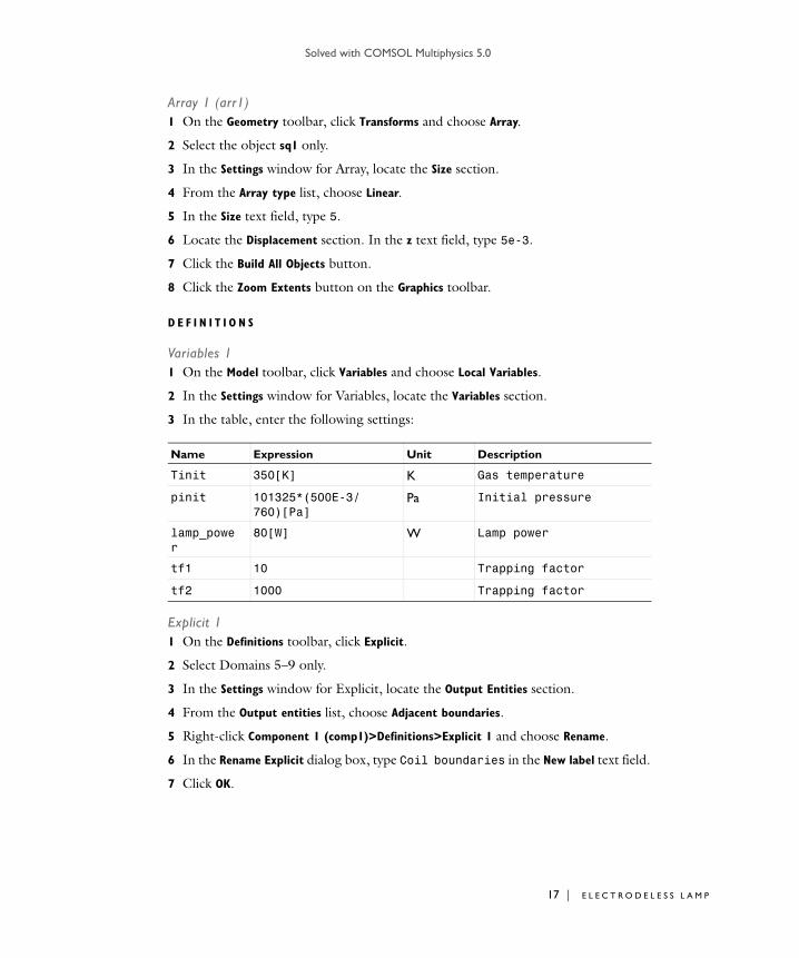
Array 1 (arr1)1 On the Geometry toolbar, click Transforms and choose Array.
2 Select the object sq1 only.
3 In the Settings window for Array, locate the Size section.
4 From the Array type list, choose Linear.
5 In the Size text field, type 5.
6 Locate the Displacement section. In the z text field, type 5e-3.
7 Click the Build All Objects button.
8 Click the Zoom Extents button on the Graphics toolbar.
D E F I N I T I O N S
Variables 11 On the Model toolbar, click Variables and choose Local Variables.
2 In the Settings window for Variables, locate the Variables section.
3 In the table, enter the following settings:
Explicit 11 On the Definitions toolbar, click Explicit.
2 Select Domains 5–9 only.
3 In the Settings window for Explicit, locate the Output Entities section.
4 From the Output entities list, choose Adjacent boundaries.
5 Right-click Component 1 (comp1)>Definitions>Explicit 1 and choose Rename.
6 In the Rename Explicit dialog box, type Coil boundaries in the New label text field.
7 Click OK.
Name Expression Unit Description
Tinit 350[K] K Gas temperature
pinit 101325*(500E-3/760)[Pa]
Pa Initial pressure
lamp_power
80[W] W Lamp power
tf1 10 Trapping factor
tf2 1000 Trapping factor
17 | E L E C T R O D E L E S S L A M P
Solved with COMSOL Multiphysics 5.0
18 | E L E
Explicit 21 On the Definitions toolbar, click Explicit.
2 Select Domains 5–9 only.
3 Right-click Component 1 (comp1)>Definitions>Explicit 2 and choose Rename.
4 In the Rename Explicit dialog box, type Coil domains in the New label text field.
5 Click OK.
Explicit 31 On the Definitions toolbar, click Explicit.
2 In the Settings window for Explicit, locate the Input Entities section.
3 From the Geometric entity level list, choose Boundary.
4 Select Boundaries 8, 27, and 35–38 only.
5 Right-click Component 1 (comp1)>Definitions>Explicit 3 and choose Rename.
6 In the Rename Explicit dialog box, type Boundary layers in the New label text field.
7 Click OK.
Explicit 41 On the Definitions toolbar, click Explicit.
2 Select Domain 4 only.
3 Right-click Component 1 (comp1)>Definitions>Explicit 4 and choose Rename.
4 In the Rename Explicit dialog box, type Discharge in the New label text field.
5 Click OK.
I N D U C T I V E L Y C O U P L E D P L A S M A ( I C P )
Cross Section Import 11 On the Physics toolbar, click Global and choose Cross Section Import.
2 In the Settings window for Cross Section Import, locate the Cross Section Import section.
3 Click Browse.
4 Browse to the model’s Model Library folder and double-click the file Ar_xsecs.txt.
Cross Section Import 21 On the Physics toolbar, click Global and choose Cross Section Import.
C T R O D E L E S S L A M P
Solved with COMSOL Multiphysics 5.0
2 In the Settings window for Cross Section Import, locate the Cross Section Import section.
3 Click Browse.
4 Browse to the model’s Model Library folder and double-click the file Hg_xsecs.txt.
Reaction 11 On the Physics toolbar, click Domains and choose Reaction.
2 In the Settings window for Reaction, locate the Reaction Formula section.
3 In the Formula text field, type Ars+Ars=>Ar++Ar+e.
4 Locate the Kinetics Expressions section. In the kf text field, type N_A_const*1.00E-15.
Reaction 21 On the Physics toolbar, click Domains and choose Reaction.
2 In the Settings window for Reaction, locate the Reaction Formula section.
3 In the Formula text field, type Ars+Hg=>Hg++Ar+e.
4 Locate the Kinetics Expressions section. In the kf text field, type N_A_const*9E-16.
58: Ars+Hg=>Hg++Ar+e1 Right-click Component 1 (comp1)>Inductively Coupled Plasma (icp)>Reaction 2 and
choose Duplicate.
2 In the Settings window for Reaction, locate the Reaction Formula section.
3 In the Formula text field, type Ars+Hg1=>Hg++Ar+e.
59: Ars+Hg1=>Hg++Ar+e1 Right-click Component 1 (comp1)>Inductively Coupled Plasma (icp)>58:
Ars+Hg=>Hg++Ar+e and choose Duplicate.
2 In the Settings window for Reaction, locate the Reaction Formula section.
3 In the Formula text field, type Ars+Hg2=>Hg++Ar+e.
60: Ars+Hg2=>Hg++Ar+e1 Right-click Component 1 (comp1)>Inductively Coupled Plasma (icp)>59:
Ars+Hg1=>Hg++Ar+e and choose Duplicate.
2 In the Settings window for Reaction, locate the Reaction Formula section.
3 In the Formula text field, type Ars+Hg3=>Hg++Ar+e.
19 | E L E C T R O D E L E S S L A M P
Solved with COMSOL Multiphysics 5.0
20 | E L E
61: Ars+Hg3=>Hg++Ar+e1 Right-click Component 1 (comp1)>Inductively Coupled Plasma (icp)>60:
Ars+Hg2=>Hg++Ar+e and choose Duplicate.
2 In the Settings window for Reaction, locate the Reaction Formula section.
3 In the Formula text field, type Ars+Hg4=>Hg++Ar+e.
62: Ars+Hg4=>Hg++Ar+e1 Right-click Component 1 (comp1)>Inductively Coupled Plasma (icp)>61:
Ars+Hg3=>Hg++Ar+e and choose Duplicate.
2 In the Settings window for Reaction, locate the Reaction Formula section.
3 In the Formula text field, type Ars+Hg5=>Hg++Ar+e.
63: Ars+Hg5=>Hg++Ar+e1 Right-click Component 1 (comp1)>Inductively Coupled Plasma (icp)>62:
Ars+Hg4=>Hg++Ar+e and choose Duplicate.
2 In the Settings window for Reaction, locate the Reaction Formula section.
3 In the Formula text field, type Ars+Hg6=>Hg++Ar+e.
64: Ars+Hg6=>Hg++Ar+e1 Right-click Component 1 (comp1)>Inductively Coupled Plasma (icp)>63:
Ars+Hg5=>Hg++Ar+e and choose Duplicate.
2 In the Settings window for Reaction, locate the Reaction Formula section.
3 In the Formula text field, type Hg3+Hg3=>Hg++Hg+e.
4 Locate the Kinetics Expressions section. In the kf text field, type N_A_const*3.50E-16.
65: Hg3+Hg3=>Hg++Hg+e1 Right-click Component 1 (comp1)>Inductively Coupled Plasma (icp)>64:
Ars+Hg6=>Hg++Ar+e and choose Duplicate.
2 In the Settings window for Reaction, locate the Reaction Formula section.
3 In the Formula text field, type Hg3+Hg4=>Hg++Hg+e.
66: Hg3+Hg4=>Hg++Hg+e1 Right-click Component 1 (comp1)>Inductively Coupled Plasma (icp)>65:
Hg3+Hg3=>Hg++Hg+e and choose Duplicate.
2 In the Settings window for Reaction, locate the Reaction Formula section.
3 In the Formula text field, type Hg3+Hg5=>Hg++Hg+e.
C T R O D E L E S S L A M P

Solved with COMSOL Multiphysics 5.0
67: Hg3+Hg5=>Hg++Hg+e1 Right-click Component 1 (comp1)>Inductively Coupled Plasma (icp)>66:
Hg3+Hg4=>Hg++Hg+e and choose Duplicate.
2 In the Settings window for Reaction, locate the Reaction Formula section.
3 In the Formula text field, type Hg3+Hg6=>Hg++Hg+e.
68: Hg3+Hg6=>Hg++Hg+e1 Right-click Component 1 (comp1)>Inductively Coupled Plasma (icp)>67:
Hg3+Hg5=>Hg++Hg+e and choose Duplicate.
2 In the Settings window for Reaction, locate the Reaction Formula section.
3 In the Formula text field, type Hg4+Hg1=>Hg++Hg+e.
69: Hg4+Hg1=>Hg++Hg+e1 Right-click Component 1 (comp1)>Inductively Coupled Plasma (icp)>68:
Hg3+Hg6=>Hg++Hg+e and choose Duplicate.
2 In the Settings window for Reaction, locate the Reaction Formula section.
3 In the Formula text field, type Hg4+Hg2=>Hg++Hg+e.
70: Hg4+Hg2=>Hg++Hg+e1 Right-click Component 1 (comp1)>Inductively Coupled Plasma (icp)>69:
Hg4+Hg1=>Hg++Hg+e and choose Duplicate.
2 In the Settings window for Reaction, locate the Reaction Formula section.
3 In the Formula text field, type Hg4+Hg3=>Hg++Hg+e.
71: Hg4+Hg3=>Hg++Hg+e1 Right-click Component 1 (comp1)>Inductively Coupled Plasma (icp)>70:
Hg4+Hg2=>Hg++Hg+e and choose Duplicate.
2 In the Settings window for Reaction, locate the Reaction Formula section.
3 In the Formula text field, type Hg4+Hg4=>Hg++Hg+e.
72: Hg4+Hg4=>Hg++Hg+e1 Right-click Component 1 (comp1)>Inductively Coupled Plasma (icp)>71:
Hg4+Hg3=>Hg++Hg+e and choose Duplicate.
2 In the Settings window for Reaction, locate the Reaction Formula section.
3 In the Formula text field, type Hg4+Hg5=>Hg++Hg+e.
21 | E L E C T R O D E L E S S L A M P
Solved with COMSOL Multiphysics 5.0
22 | E L E
73: Hg4+Hg5=>Hg++Hg+e1 Right-click Component 1 (comp1)>Inductively Coupled Plasma (icp)>72:
Hg4+Hg4=>Hg++Hg+e and choose Duplicate.
2 In the Settings window for Reaction, locate the Reaction Formula section.
3 In the Formula text field, type Hg4+Hg6=>Hg++Hg+e.
74: Hg4+Hg6=>Hg++Hg+e1 Right-click Component 1 (comp1)>Inductively Coupled Plasma (icp)>73:
Hg4+Hg5=>Hg++Hg+e and choose Duplicate.
2 In the Settings window for Reaction, locate the Reaction Formula section.
3 In the Formula text field, type Hg5+Hg1=>Hg++Hg+e.
75: Hg5+Hg1=>Hg++Hg+e1 Right-click Component 1 (comp1)>Inductively Coupled Plasma (icp)>74:
Hg4+Hg6=>Hg++Hg+e and choose Duplicate.
2 In the Settings window for Reaction, locate the Reaction Formula section.
3 In the Formula text field, type Hg5+Hg2=>Hg++Hg+e.
76: Hg5+Hg2=>Hg++Hg+e1 Right-click Component 1 (comp1)>Inductively Coupled Plasma (icp)>75:
Hg5+Hg1=>Hg++Hg+e and choose Duplicate.
2 In the Settings window for Reaction, locate the Reaction Formula section.
3 In the Formula text field, type Hg5+Hg3=>Hg++Hg+e.
77: Hg5+Hg3=>Hg++Hg+e1 Right-click Component 1 (comp1)>Inductively Coupled Plasma (icp)>76:
Hg5+Hg2=>Hg++Hg+e and choose Duplicate.
2 In the Settings window for Reaction, locate the Reaction Formula section.
3 In the Formula text field, type Hg5+Hg4=>Hg++Hg+e.
78: Hg5+Hg4=>Hg++Hg+e1 Right-click Component 1 (comp1)>Inductively Coupled Plasma (icp)>77:
Hg5+Hg3=>Hg++Hg+e and choose Duplicate.
2 In the Settings window for Reaction, locate the Reaction Formula section.
3 In the Formula text field, type Hg5+Hg5=>Hg++Hg+e.
C T R O D E L E S S L A M P
Solved with COMSOL Multiphysics 5.0
79: Hg5+Hg5=>Hg++Hg+e1 Right-click Component 1 (comp1)>Inductively Coupled Plasma (icp)>78:
Hg5+Hg4=>Hg++Hg+e and choose Duplicate.
2 In the Settings window for Reaction, locate the Reaction Formula section.
3 In the Formula text field, type Hg5+Hg6=>Hg++Hg+e.
80: Hg5+Hg6=>Hg++Hg+e1 Right-click Component 1 (comp1)>Inductively Coupled Plasma (icp)>79:
Hg5+Hg5=>Hg++Hg+e and choose Duplicate.
2 In the Settings window for Reaction, locate the Reaction Formula section.
3 In the Formula text field, type Hg6+Hg1=>Hg++Hg+e.
81: Hg6+Hg1=>Hg++Hg+e1 Right-click Component 1 (comp1)>Inductively Coupled Plasma (icp)>80:
Hg5+Hg6=>Hg++Hg+e and choose Duplicate.
2 In the Settings window for Reaction, locate the Reaction Formula section.
3 In the Formula text field, type Hg6+Hg2=>Hg++Hg+e.
82: Hg6+Hg2=>Hg++Hg+e1 Right-click Component 1 (comp1)>Inductively Coupled Plasma (icp)>81:
Hg6+Hg1=>Hg++Hg+e and choose Duplicate.
2 In the Settings window for Reaction, locate the Reaction Formula section.
3 In the Formula text field, type Hg6+Hg3=>Hg++Hg+e.
83: Hg6+Hg3=>Hg++Hg+e1 Right-click Component 1 (comp1)>Inductively Coupled Plasma (icp)>82:
Hg6+Hg2=>Hg++Hg+e and choose Duplicate.
2 In the Settings window for Reaction, locate the Reaction Formula section.
3 In the Formula text field, type Hg6+Hg4=>Hg++Hg+e.
84: Hg6+Hg4=>Hg++Hg+e1 Right-click Component 1 (comp1)>Inductively Coupled Plasma (icp)>83:
Hg6+Hg3=>Hg++Hg+e and choose Duplicate.
2 In the Settings window for Reaction, locate the Reaction Formula section.
3 In the Formula text field, type Hg6+Hg5=>Hg++Hg+e.
23 | E L E C T R O D E L E S S L A M P
Solved with COMSOL Multiphysics 5.0
24 | E L E
85: Hg6+Hg5=>Hg++Hg+e1 Right-click Component 1 (comp1)>Inductively Coupled Plasma (icp)>84:
Hg6+Hg4=>Hg++Hg+e and choose Duplicate.
2 In the Settings window for Reaction, locate the Reaction Formula section.
3 In the Formula text field, type Hg6+Hg6=>Hg++Hg+e.
86: Hg6+Hg6=>Hg++Hg+e1 Right-click Component 1 (comp1)>Inductively Coupled Plasma (icp)>85:
Hg6+Hg5=>Hg++Hg+e and choose Duplicate.
2 In the Settings window for Reaction, locate the Reaction Formula section.
3 In the Formula text field, type Ar++Hg=>Hg++Ar.
4 Locate the Kinetics Expressions section. In the kf text field, type N_A_const*1.50E-17.
87: Ar++Hg=>Hg++Ar1 Right-click Component 1 (comp1)>Inductively Coupled Plasma (icp)>86:
Hg6+Hg6=>Hg++Hg+e and choose Duplicate.
2 In the Settings window for Reaction, locate the Reaction Formula section.
3 In the Formula text field, type Ar++Ar=>Ar++Ar.
4 Locate the Kinetics Expressions section. In the kf text field, type N_A_const*4.60E-16.
88: Ar++Ar=>Ar++Ar1 Right-click Component 1 (comp1)>Inductively Coupled Plasma (icp)>87:
Ar++Hg=>Hg++Ar and choose Duplicate.
2 In the Settings window for Reaction, locate the Reaction Formula section.
3 In the Formula text field, type Hg++Hg=>Hg+Hg+.
4 Locate the Kinetics Expressions section. In the kf text field, type N_A_const*1.00E-15.
89: Hg++Hg=>Hg+Hg+1 Right-click Component 1 (comp1)>Inductively Coupled Plasma (icp)>88:
Ar++Ar=>Ar++Ar and choose Duplicate.
2 In the Settings window for Reaction, locate the Reaction Formula section.
3 In the Formula text field, type Hg2=>Hg.
4 Locate the Kinetics Expressions section. In the kf text field, type 8.00E6/tf1.
C T R O D E L E S S L A M P
Solved with COMSOL Multiphysics 5.0
90: Hg2=>Hg1 Right-click Component 1 (comp1)>Inductively Coupled Plasma (icp)>89:
Hg++Hg=>Hg+Hg+ and choose Duplicate.
2 In the Settings window for Reaction, locate the Reaction Formula section.
3 In the Formula text field, type Hg4=>Hg.
4 Locate the Kinetics Expressions section. In the kf text field, type 7.50E8/tf2.
91: Hg4=>Hg1 Right-click Component 1 (comp1)>Inductively Coupled Plasma (icp)>90: Hg2=>Hg and
choose Duplicate.
2 In the Settings window for Reaction, locate the Reaction Formula section.
3 In the Formula text field, type Hg5=>Hg1.
4 Locate the Kinetics Expressions section. In the kf text field, type 2.2E7.
92: Hg5=>Hg11 Right-click Component 1 (comp1)>Inductively Coupled Plasma (icp)>91: Hg4=>Hg and
choose Duplicate.
2 In the Settings window for Reaction, locate the Reaction Formula section.
3 In the Formula text field, type Hg5=>Hg2.
4 Locate the Kinetics Expressions section. In the kf text field, type 6.6E7.
93: Hg5=>Hg21 Right-click Component 1 (comp1)>Inductively Coupled Plasma (icp)>92: Hg5=>Hg1
and choose Duplicate.
2 In the Settings window for Reaction, locate the Reaction Formula section.
3 In the Formula text field, type Hg5=>Hg3.
4 Locate the Kinetics Expressions section. In the kf text field, type 2E7.
94: Hg5=>Hg31 Right-click Component 1 (comp1)>Inductively Coupled Plasma (icp)>93: Hg5=>Hg2
and choose Duplicate.
2 In the Settings window for Reaction, locate the Reaction Formula section.
3 In the Formula text field, type Hg6=>Hg1.
95: Hg6=>Hg11 Right-click Component 1 (comp1)>Inductively Coupled Plasma (icp)>94: Hg5=>Hg3
and choose Duplicate.
25 | E L E C T R O D E L E S S L A M P
Solved with COMSOL Multiphysics 5.0
26 | E L E
2 In the Settings window for Reaction, locate the Reaction Formula section.
3 In the Formula text field, type Hg6=>Hg2.
4 Locate the Kinetics Expressions section. In the kf text field, type 6E7.
96: Hg6=>Hg21 Right-click Component 1 (comp1)>Inductively Coupled Plasma (icp)>95: Hg6=>Hg1
and choose Duplicate.
2 In the Settings window for Reaction, locate the Reaction Formula section.
3 In the Formula text field, type Hg6=>Hg3.
4 Locate the Kinetics Expressions section. In the kf text field, type 5E7.
Surface Reaction 11 On the Physics toolbar, click Boundaries and choose Surface Reaction.
2 In the Settings window for Surface Reaction, locate the Reaction Formula section.
3 In the Formula text field, type Ars=>Ar.
4 Locate the Boundary Selection section. From the Selection list, choose Boundary
layers.
2: Ars=>Ar1 Right-click Component 1 (comp1)>Inductively Coupled Plasma (icp)>Surface Reaction
1 and choose Duplicate.
2 In the Settings window for Surface Reaction, locate the Reaction Formula section.
3 In the Formula text field, type Ar+=>Ar.
3: Ar+=>Ar1 Right-click Component 1 (comp1)>Inductively Coupled Plasma (icp)>2: Ars=>Ar and
choose Duplicate.
2 In the Settings window for Surface Reaction, locate the Reaction Formula section.
3 In the Formula text field, type Hg1=>Hg.
4: Hg1=>Hg1 Right-click Component 1 (comp1)>Inductively Coupled Plasma (icp)>3: Ar+=>Ar and
choose Duplicate.
2 In the Settings window for Surface Reaction, locate the Reaction Formula section.
3 In the Formula text field, type Hg2=>Hg.
C T R O D E L E S S L A M P
Solved with COMSOL Multiphysics 5.0
5: Hg2=>Hg1 Right-click Component 1 (comp1)>Inductively Coupled Plasma (icp)>4: Hg1=>Hg and
choose Duplicate.
2 In the Settings window for Surface Reaction, locate the Reaction Formula section.
3 In the Formula text field, type Hg3=>Hg.
6: Hg3=>Hg1 Right-click Component 1 (comp1)>Inductively Coupled Plasma (icp)>5: Hg2=>Hg and
choose Duplicate.
2 In the Settings window for Surface Reaction, locate the Reaction Formula section.
3 In the Formula text field, type Hg4=>Hg.
7: Hg4=>Hg1 Right-click Component 1 (comp1)>Inductively Coupled Plasma (icp)>6: Hg3=>Hg and
choose Duplicate.
2 In the Settings window for Surface Reaction, locate the Reaction Formula section.
3 In the Formula text field, type Hg5=>Hg.
8: Hg5=>Hg1 Right-click Component 1 (comp1)>Inductively Coupled Plasma (icp)>7: Hg4=>Hg and
choose Duplicate.
2 In the Settings window for Surface Reaction, locate the Reaction Formula section.
3 In the Formula text field, type Hg6=>Hg.
9: Hg6=>Hg1 Right-click Component 1 (comp1)>Inductively Coupled Plasma (icp)>8: Hg5=>Hg and
choose Duplicate.
2 In the Settings window for Surface Reaction, locate the Reaction Formula section.
3 In the Formula text field, type Hg+=>Hg.
Species: Hg1 In the Model Builder window, under Component 1 (comp1)>Inductively Coupled
Plasma (icp) click Species: Hg.
2 In the Settings window for Species, locate the General Parameters section.
3 In the Mw text field, type 0.2006.
4 In the σ text field, type 2.969[angstrom].
5 In the ε/kb text field, type 750.
27 | E L E C T R O D E L E S S L A M P
Solved with COMSOL Multiphysics 5.0
28 | E L E
6 In the x0 text field, type 0.05.
Species: Hg11 In the Model Builder window, under Component 1 (comp1)>Inductively Coupled
Plasma (icp) click Species: Hg1.
2 In the Settings window for Species, locate the General Parameters section.
3 In the Mw text field, type 0.2006.
4 In the σ text field, type 2.969[angstrom].
5 In the ε/kb text field, type 750.
6 In the x0 text field, type 2E-6.
Species: Hg21 In the Model Builder window, under Component 1 (comp1)>Inductively Coupled
Plasma (icp) click Species: Hg2.
2 In the Settings window for Species, locate the General Parameters section.
3 In the Mw text field, type 0.2006.
4 In the σ text field, type 2.969[angstrom].
5 In the ε/kb text field, type 750.
6 In the x0 text field, type 1E-6.
Species: Hg31 In the Model Builder window, under Component 1 (comp1)>Inductively Coupled
Plasma (icp) click Species: Hg3.
2 In the Settings window for Species, locate the General Parameters section.
3 In the Mw text field, type 0.2006.
4 In the σ text field, type 2.969[angstrom].
5 In the ε/kb text field, type 750.
6 In the x0 text field, type 5E-6.
Species: Hg41 In the Model Builder window, under Component 1 (comp1)>Inductively Coupled
Plasma (icp) click Species: Hg4.
2 In the Settings window for Species, locate the General Parameters section.
3 In the Mw text field, type 0.2006.
4 In the σ text field, type 2.969[angstrom].
5 In the ε/kb text field, type 750.
C T R O D E L E S S L A M P
Solved with COMSOL Multiphysics 5.0
6 In the x0 text field, type 1E-6.
Species: Hg51 In the Model Builder window, under Component 1 (comp1)>Inductively Coupled
Plasma (icp) click Species: Hg5.
2 In the Settings window for Species, locate the General Parameters section.
3 In the Mw text field, type 0.2006.
4 In the σ text field, type 2.969[angstrom].
5 In the ε/kb text field, type 750.
6 In the x0 text field, type 5E-6.
Species: Hg61 In the Model Builder window, under Component 1 (comp1)>Inductively Coupled
Plasma (icp) click Species: Hg6.
2 In the Settings window for Species, locate the General Parameters section.
3 In the Mw text field, type 0.2006.
4 In the σ text field, type 2.969[angstrom].
5 In the ε/kb text field, type 750.
6 In the x0 text field, type 1E-6.
Species: Ar1 In the Model Builder window, under Component 1 (comp1)>Inductively Coupled
Plasma (icp) click Species: Ar.
2 In the Settings window for Species, locate the Species Formula section.
3 Select the From mass constraint check box.
Species: Ar+1 In the Model Builder window, under Component 1 (comp1)>Inductively Coupled
Plasma (icp) click Species: Ar+.
2 In the Settings window for Species, locate the General Parameters section.
3 In the n0 text field, type 1E16.
Species: Hg+1 In the Model Builder window, under Component 1 (comp1)>Inductively Coupled
Plasma (icp) click Species: Hg+.
2 In the Settings window for Species, locate the General Parameters section.
3 In the Mw text field, type 0.2006.
29 | E L E C T R O D E L E S S L A M P
Solved with COMSOL Multiphysics 5.0
30 | E L E
4 In the σ text field, type 2.969[angstrom].
5 In the ε/kb text field, type 750.
6 Locate the Species Formula section. Select the Initial value from electroneutrality
constraint check box.
Plasma Model 11 In the Model Builder window, under Component 1 (comp1)>Inductively Coupled
Plasma (icp) click Plasma Model 1.
2 In the Settings window for Plasma Model, locate the Electron Density and Energy section.
3 In the μe text field, type 4E24[1/(m*V*s)]/icp.Nn.
4 Locate the Model Inputs section. In the T text field, type Tinit.
5 In the pA text field, type pinit.
Ampère's Law 11 On the Physics toolbar, click Domains and choose Ampère's Law.
2 Select Domains 1–3 and 5–9 only.
Ground 11 On the Physics toolbar, click Boundaries and choose Ground.
2 In the Settings window for Ground, locate the Boundary Selection section.
3 From the Selection list, choose Boundary layers.
Wall 11 On the Physics toolbar, click Boundaries and choose Wall.
2 In the Settings window for Wall, locate the Boundary Selection section.
3 From the Selection list, choose Boundary layers.
Initial Values 11 In the Model Builder window, under Component 1 (comp1)>Inductively Coupled
Plasma (icp) click Initial Values 1.
2 In the Settings window for Initial Values, locate the Initial Values section.
3 In the ne,0 text field, type 1E17.
4 In the ε0 text field, type 2.
5 Click the Zoom Box button on the Graphics toolbar.
Coil Group Domain 11 On the Physics toolbar, click Domains and choose Coil Group Domain.
C T R O D E L E S S L A M P
Solved with COMSOL Multiphysics 5.0
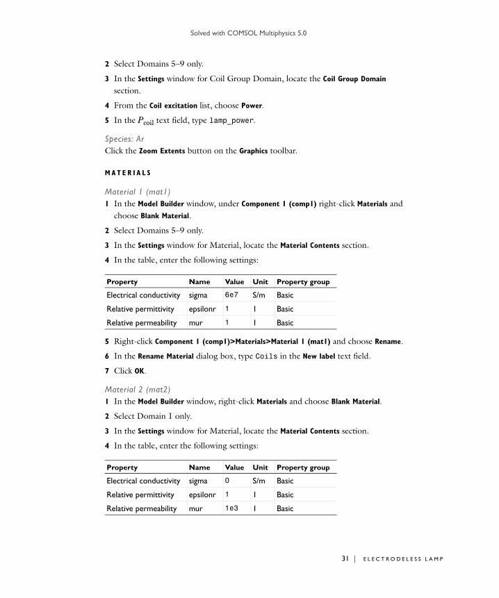
2 Select Domains 5–9 only.
3 In the Settings window for Coil Group Domain, locate the Coil Group Domain section.
4 From the Coil excitation list, choose Power.
5 In the Pcoil text field, type lamp_power.
Species: ArClick the Zoom Extents button on the Graphics toolbar.
M A T E R I A L S
Material 1 (mat1)1 In the Model Builder window, under Component 1 (comp1) right-click Materials and
choose Blank Material.
2 Select Domains 5–9 only.
3 In the Settings window for Material, locate the Material Contents section.
4 In the table, enter the following settings:
5 Right-click Component 1 (comp1)>Materials>Material 1 (mat1) and choose Rename.
6 In the Rename Material dialog box, type Coils in the New label text field.
7 Click OK.
Material 2 (mat2)1 In the Model Builder window, right-click Materials and choose Blank Material.
2 Select Domain 1 only.
3 In the Settings window for Material, locate the Material Contents section.
4 In the table, enter the following settings:
Property Name Value Unit Property group
Electrical conductivity sigma 6e7 S/m Basic
Relative permittivity epsilonr 1 1 Basic
Relative permeability mur 1 1 Basic
Property Name Value Unit Property group
Electrical conductivity sigma 0 S/m Basic
Relative permittivity epsilonr 1 1 Basic
Relative permeability mur 1e3 1 Basic
31 | E L E C T R O D E L E S S L A M P
Solved with COMSOL Multiphysics 5.0
32 | E L E
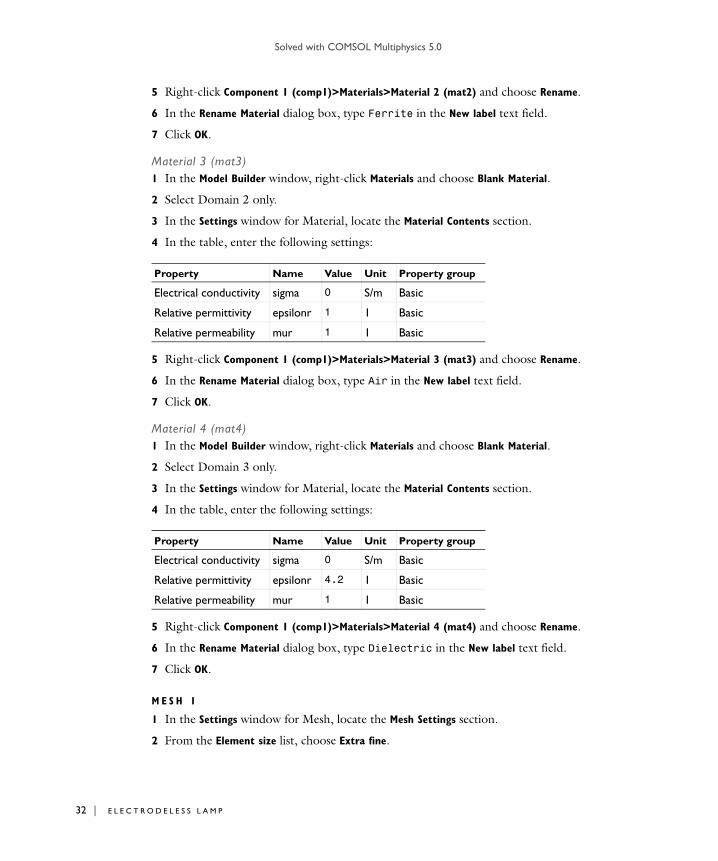
5 Right-click Component 1 (comp1)>Materials>Material 2 (mat2) and choose Rename.
6 In the Rename Material dialog box, type Ferrite in the New label text field.
7 Click OK.
Material 3 (mat3)1 In the Model Builder window, right-click Materials and choose Blank Material.
2 Select Domain 2 only.
3 In the Settings window for Material, locate the Material Contents section.
4 In the table, enter the following settings:
5 Right-click Component 1 (comp1)>Materials>Material 3 (mat3) and choose Rename.
6 In the Rename Material dialog box, type Air in the New label text field.
7 Click OK.
Material 4 (mat4)1 In the Model Builder window, right-click Materials and choose Blank Material.
2 Select Domain 3 only.
3 In the Settings window for Material, locate the Material Contents section.
4 In the table, enter the following settings:
5 Right-click Component 1 (comp1)>Materials>Material 4 (mat4) and choose Rename.
6 In the Rename Material dialog box, type Dielectric in the New label text field.
7 Click OK.
M E S H 1
1 In the Settings window for Mesh, locate the Mesh Settings section.
2 From the Element size list, choose Extra fine.
Property Name Value Unit Property group
Electrical conductivity sigma 0 S/m Basic
Relative permittivity epsilonr 1 1 Basic
Relative permeability mur 1 1 Basic
Property Name Value Unit Property group
Electrical conductivity sigma 0 S/m Basic
Relative permittivity epsilonr 4.2 1 Basic
Relative permeability mur 1 1 Basic
C T R O D E L E S S L A M P
Solved with COMSOL Multiphysics 5.0
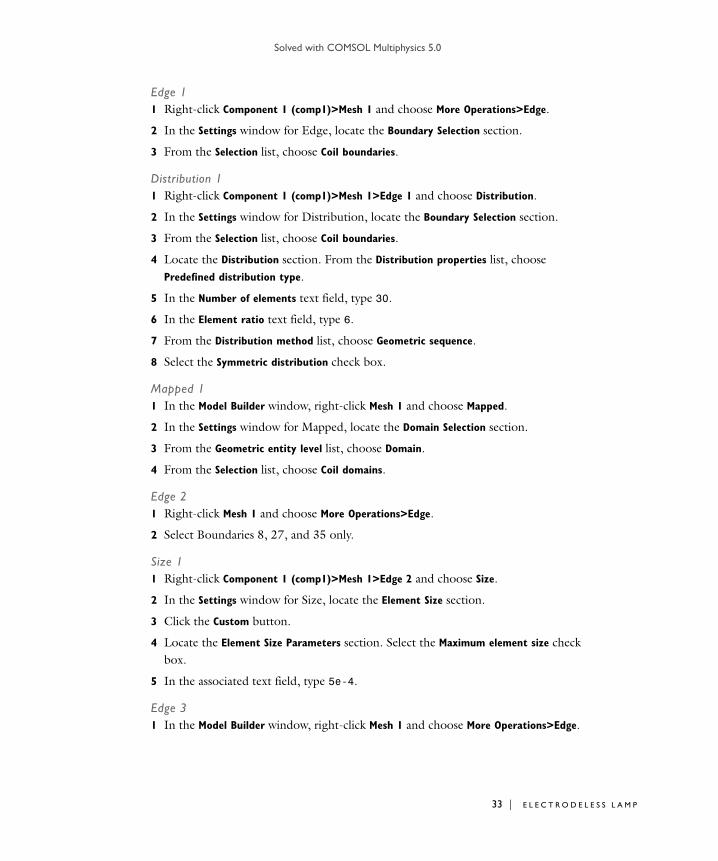
Edge 11 Right-click Component 1 (comp1)>Mesh 1 and choose More Operations>Edge.
2 In the Settings window for Edge, locate the Boundary Selection section.
3 From the Selection list, choose Coil boundaries.
Distribution 11 Right-click Component 1 (comp1)>Mesh 1>Edge 1 and choose Distribution.
2 In the Settings window for Distribution, locate the Boundary Selection section.
3 From the Selection list, choose Coil boundaries.
4 Locate the Distribution section. From the Distribution properties list, choose Predefined distribution type.
5 In the Number of elements text field, type 30.
6 In the Element ratio text field, type 6.
7 From the Distribution method list, choose Geometric sequence.
8 Select the Symmetric distribution check box.
Mapped 11 In the Model Builder window, right-click Mesh 1 and choose Mapped.
2 In the Settings window for Mapped, locate the Domain Selection section.
3 From the Geometric entity level list, choose Domain.
4 From the Selection list, choose Coil domains.
Edge 21 Right-click Mesh 1 and choose More Operations>Edge.
2 Select Boundaries 8, 27, and 35 only.
Size 11 Right-click Component 1 (comp1)>Mesh 1>Edge 2 and choose Size.
2 In the Settings window for Size, locate the Element Size section.
3 Click the Custom button.
4 Locate the Element Size Parameters section. Select the Maximum element size check box.
5 In the associated text field, type 5e-4.
Edge 31 In the Model Builder window, right-click Mesh 1 and choose More Operations>Edge.
33 | E L E C T R O D E L E S S L A M P
Solved with COMSOL Multiphysics 5.0
34 | E L E
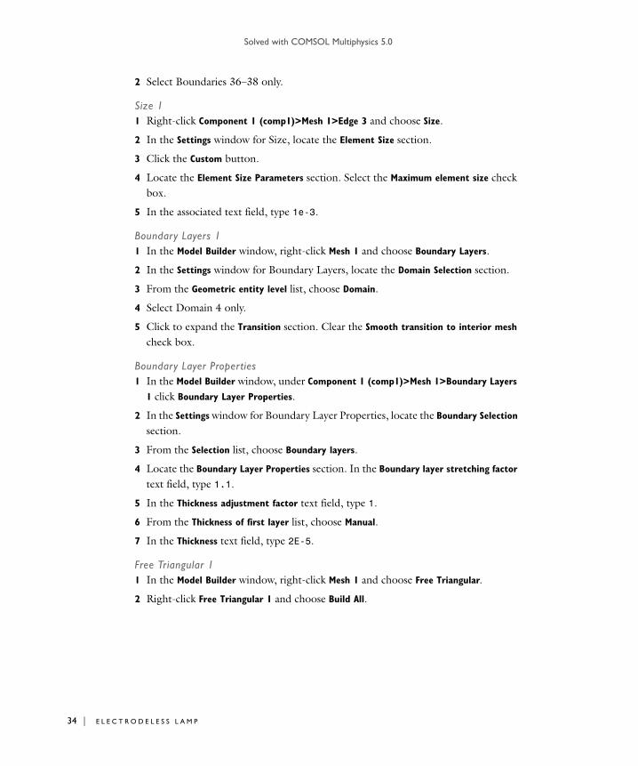
2 Select Boundaries 36–38 only.
Size 11 Right-click Component 1 (comp1)>Mesh 1>Edge 3 and choose Size.
2 In the Settings window for Size, locate the Element Size section.
3 Click the Custom button.
4 Locate the Element Size Parameters section. Select the Maximum element size check box.
5 In the associated text field, type 1e-3.
Boundary Layers 11 In the Model Builder window, right-click Mesh 1 and choose Boundary Layers.
2 In the Settings window for Boundary Layers, locate the Domain Selection section.
3 From the Geometric entity level list, choose Domain.
4 Select Domain 4 only.
5 Click to expand the Transition section. Clear the Smooth transition to interior mesh check box.
Boundary Layer Properties1 In the Model Builder window, under Component 1 (comp1)>Mesh 1>Boundary Layers
1 click Boundary Layer Properties.
2 In the Settings window for Boundary Layer Properties, locate the Boundary Selection section.
3 From the Selection list, choose Boundary layers.
4 Locate the Boundary Layer Properties section. In the Boundary layer stretching factor text field, type 1.1.
5 In the Thickness adjustment factor text field, type 1.
6 From the Thickness of first layer list, choose Manual.
7 In the Thickness text field, type 2E-5.
Free Triangular 11 In the Model Builder window, right-click Mesh 1 and choose Free Triangular.
2 Right-click Free Triangular 1 and choose Build All.
C T R O D E L E S S L A M P
Solved with COMSOL Multiphysics 5.0
S T U D Y 1
Step 1: Frequency-Transient1 In the Model Builder window, expand the Study 1 node, then click Step 1:
Frequency-Transient.
2 In the Settings window for Frequency-Transient, locate the Study Settings section.
3 In the Frequency text field, type 2[MHz].
4 In the Times text field, type 0.
5 Click Range.
6 In the Range dialog box, choose Number of values from the Entry method list.
7 In the Start text field, type -8.
8 In the Stop text field, type log10(2e-3).
9 In the Number of values text field, type 3.
10 From the Function to apply to all values list, choose exp10.
11 Click Add.
12 On the Model toolbar, click Compute.
R E S U L T S
2D Plot Group 41 On the Model toolbar, click Add Plot Group and choose 2D Plot Group.
2 In the Model Builder window, under Results right-click 2D Plot Group 4 and choose Surface.
3 In the Settings window for Surface, click Replace Expression in the upper-right corner of the Expression section. From the menu, choose Component 1>Inductively Coupled
Plasma (Magnetic Fields)>Heating and losses>icp.Qrh - Resistive losses.
4 On the 2D plot group toolbar, click Plot.
2D Plot Group 51 On the Model toolbar, click Add Plot Group and choose 2D Plot Group.
2 In the Model Builder window, under Results right-click 2D Plot Group 5 and choose Surface.
3 In the Settings window for Surface, click Replace Expression in the upper-right corner of the Expression section. From the menu, choose Component 1>Inductively Coupled
Plasma (Heavy Species Transport)>Mole fractions>icp.x_wHg - Mole fraction.
4 On the 2D plot group toolbar, click Plot.
35 | E L E C T R O D E L E S S L A M P
Solved with COMSOL Multiphysics 5.0
36 | E L E
2D Plot Group 61 On the Model toolbar, click Add Plot Group and choose 2D Plot Group.
2 In the Model Builder window, under Results right-click 2D Plot Group 6 and choose Surface.
3 In the Settings window for Surface, click Replace Expression in the upper-right corner of the Expression section. From the menu, choose Component 1>Inductively Coupled
Plasma (Heavy Species Transport)>Number densities>icp.n_wHg_1p - Number density.
4 On the 2D plot group toolbar, click Plot.
2D Plot Group 71 On the Model toolbar, click Add Plot Group and choose 2D Plot Group.
2 In the Model Builder window, under Results right-click 2D Plot Group 7 and choose Surface.
3 In the Settings window for Surface, click Replace Expression in the upper-right corner of the Expression section. From the menu, choose Component 1>Inductively Coupled
Plasma (Heavy Species Transport)>Mole fractions>icp.x_wHg2 - Mole fraction.
4 On the 2D plot group toolbar, click Plot.
2D Plot Group 81 On the Model toolbar, click Add Plot Group and choose 2D Plot Group.
2 In the Model Builder window, under Results right-click 2D Plot Group 8 and choose Surface.
3 In the Settings window for Surface, click Replace Expression in the upper-right corner of the Expression section. From the menu, choose Component 1>Inductively Coupled
Plasma (Heavy Species Transport)>Mole fractions>icp.x_wHg4 - Mole fraction.
4 On the 2D plot group toolbar, click Plot.
C T R O D E L E S S L A M P