modelling systems by hybrid petri nets: an application … · · 2008-01-10modelling systems by...

5

Modelling Systems by Hybrid Petri Nets: an Application to Supply Chains

Mariagrazia Dotoli1, Maria Pia Fanti1, Alessandro Giua2, Carla Seatzu2 1Dip. di Elettrotecnica ed Elettronica, Politecnico di Bari,

2Dip. di Ingegneria Elettrica ed Elettronica, Università degli Studi di Cagliari Italy

1. Introduction Petri Nets (PNs) are a discrete event model firstly proposed by Carl Adam Petri in his Ph.D. thesis in the early 1960s (Petri, 1962). The main feature of a (discrete) PN is that its state is a vector of non-negative integers. This is a major advantage with respect to other formalisms such as automata, where the state space is a symbolic unstructured set, and has been exploited to develop many analysis techniques that do not require to enumerate the state space (structural analysis) (Silva et al., 1996). Another key feature of PNs is their capacity to graphically represent and visualize primitives such as parallelism, concurrency, synchronization, mutual exclusion, etc. In the related literature various PN extensions have been proposed. In this paper we focus on Continuous and Hybrid PNs. Continuous Petri Nets (CPNs) originate from the “fluidification” of discrete PNs (David & Alla, 1987). In simple words, the content of places is relaxed to be a real non-negative number rather than an integer non-negative number, and appropriate rules for transitions firings are given. This highly reduces the computational complexity of the analysis and optimization of realistic scale problems, and has been successfully applied to manufacturing systems. The main advantages of fluidification can be summarized in the following four items. • The computational complexity of the analysis and control of complex systems may be

significantly reduced. • Fluid approximations provide an aggregate formulation to deal with complex systems,

thus reducing the dimension of the state space. The resulting simple structures allow explicit computation and performance optimization.

• The design parameters in fluid models are continuous; hence, it is possible to use gradient information to speed up optimization and to perform sensitivity analysis.

• Finally, in many cases it has also been shown that fluid approximations do not introduce significant errors when carrying out performance analysis via simulation.

In general, different fluid approximations are necessary to describe the same system, depending on its discrete state, e.g., in the manufacturing domain, machines working or down, buffers full or empty, and so on. Thus, the resulting model can be better described as a hybrid model, where a different continuous dynamics is associated to each discrete state. Hybrid Petri Nets (HPNs) keep all those good features that make discrete PNs a valuable

Petri Net: Theory and Applications 358

discrete-event model: they do not require the exhaustive enumeration of the state space and can finitely describe systems with an infinite state space; they allow modular representation where the structure of each module is kept in the composed model; the discrete state is represented by a vector and not by a symbolic label, thus linear algebraic techniques may be used for their analysis. Different HPN models have been proposed in the literature, but there is so far no widely accepted classification of such models. In Section 2 we provide a brief survey of the most important HPN models presented in the related literature. The main theoretical results and the main application areas within each framework are also mentioned. We recently provided a more detailed survey in (Dotoli et al., 2007). In Section 3 we focus our attention on a particular model of HPNs, called First-Order Hybrid Petri Nets (FOHPNs) because its continuous dynamics are piece-wise constant. FOHPNs were originally proposed in (Balduzzi et al., 2000) and have been efficiently used in many application domains, such as manufacturing systems (Balduzzi et al., 2001; Giua et al., 2005) and inventory control (Furcas et al., 2001). Interesting optimization problems have also been studied considering real applications, such as a bottling plant (Giua et al., 2005) and a cheese factory (Furcas et al. 2001). Finally, in Section 4 we show how FOHPNs can be efficiently used for modelling and controlling large and complex systems such as Supply Chains (SCs). SCs are complex emerging distributed manufacturing systems whose analysis, design and management is currently an active area of research (Viswanadham & Gaonkar, 2003; Viswanadham & Raghavan, 2000; Dotoli et al., 2005; Dotoli et al., 2006). More precisely, a SC is defined as a collection of independent companies possessing complementary skills and integrated with transportation and storage systems, information and financial flows, with all entities collaborating to meet the market demand. Appropriate modelling and analysis of such highly complex systems are crucial for performance evaluation and to compare competing SC. However, in the related literature few contributions deal with the problem of modelling and analyzing the SC operational behaviour. Viswanadham and Raghavan (2000) model SC as discrete event dynamical systems, in which the evolution depends on the interaction of discrete events such as the arrival of the components at the facilities, the departure of the transport, the start of the operations at the manufacturers and the assemblers. In (Desrochers et al., 2005) a two-product SC is modelled by complex-valued token PNs and the performance measures are determined by simulation. However, the limit of such formalisms is the modelling of products or batches of parts by means of discrete quantities (i.e., tokens). This assumption is not realistic in large SCs with a huge amount of material flow. Hence, this paper uses FOHPNs to model and manage SCs. Using a modular approach based on the idea of bottom-up methodology (Zhou & Venkatesh, 1998), this work develops a modular FOHPN model of SCs where the input buffers are managed by the well known fixed order quantity policy. In particular, transporters and manufacturers are described by continuous transitions, buffers are continuous places, and products are represented by continuous flows (fluids) routing from manufacturers, buffers and transporters.

2. Hybrid Petri nets The first fluid PN model is the so called “Continuous and Hybrid Petri Net” model introduced by David and Alla in their seminal paper (David & Alla, 1987). Based on this first formalism, and motivated by particular applications, a family of extended hybrid

Modelling Systems by Hybrid Petri Nets: an Application to Supply Chains 359

models has then been proposed in the literature. In this section we briefly recall some of them, namely Fluid Stochastic Petri Nets, Batch Nets, DAE-Petri Nets, Hybrid Flow Nets, Differential Petri Nets and High-Level Hybrid Nets. For a more detail survey on Hybrid Petri Nets (HPNs) we address the reader to (Dotoli et al. 2007) and to (David & Alla, 2005).

2.1 Continuous and hybrid Petri nets All the works collected under this heading are based on or directly inspired to the model presented by R. David and H. Alla in the late eighties (David & Alla, 1987). These authors have obtained a continuous model by fluidification, i.e., by relaxing the condition that the marking be an integer vector. Hybrid Petri nets are then made of a “continuous part” (continuous places and transitions) and a “discrete part” (discrete places and transitions). The continuous part can model systems with continuous flows and the discrete part models the logic behavior. Several contributions in this framework have been presented in the last decade, as well as some interesting extensions with respect to the original model. As an example, the problem of determining an optimal stationary mode of operation for a system described by a timed CPN has been studied in (Gaujal & Giua, 2004). Some characterizations of equilibrium points in steady-state are given in (Mahulea et al., 2007), where an optimal steady-state control is also studied. An interesting comparison on two different techniques to compute the steady-state of continuous nets was made in (Demongodin & Giua, 2002): a method based on linear programming and a method based on graph theory are considered. Other interesting papers have been devoted to the problem of production frequencies estimation for systems that are modeled by CPNs (Lefebvre, 2000), to the design of observers (Júlvez et al., 2004), to the reachability analysis (Júlvez et al., 2003), to the stability analysis (Amer-Yahia & Zerhouni, 2001), and to the deadlock-freeness analysis (Júlvez et al., 2002). The problem of deriving an optimal control law for CPNs under the assumption of finite servers semantics has been studied in (Bemporad et al., 2004). In (Mahulea et al., 2006a) the authors considered timed CPNs under infinite servers semantics that usually provide a much better approximation of the discrete system than finite servers semantics (Mahulea et al., 2006b). They deal with the problem of controlling CPNs in order to reach a final (steady state) configuration while minimizing a quadratic performance index. CPNs have been mainly applied in the manufacturing domain (for an exhaustive list of references see (Dotoli et al., 2007)), even if some other interesting applications have been presented, like (Amer-Yahia et al., 1997) dealing with biological systems, and (Júlvez & Boel, 2005) dealing with transportation systems. FOHPNs follow the formalism described in (Alla & David, 1998) with the addition of algebraic analysis techniques, and have been firstly presented in (Balduzzi et al., 2000). FOHPNs consist of continuous places holding fluid, discrete places containing a non-negative integer number of tokens, and transitions, either discrete or continuous. As in all hybrid models, in FOHPNs the authors distinguish two behavioral levels: time-driven and event-driven. The continuous time-driven evolution of the net is described by first-order fluid models, i.e., models in which the continuous flows have constant rates and the fluid content of each continuous place varies linearly with time. A discrete-event model describes the behaviour of the net that, upon the occurrence of macro-events, evolves through a


sequence of macro-states. The authors set up a linear algebraic formalism to study the first--order continuous behavior of this model and show how its control can be framed as a conflict resolution policy that aims at optimizing a given objective function. The use of linear algebra leads to sensitivity analysis that allows one to study how changes in the structure of the model influence the optimal behavior. This model is extensively presented in the rest of this paper.

2.2 Other models The Fluid Stochastic Petri Net (FSPN) model has been firstly presented by K.S. Trivedi and V.G. Kulkarni in the early nineties (Trivedi & Kulkarni, 1993). Here the authors extend the stochastic Petri nets framework (Ajmone Marsan et al., 1995) to FSPNs by introducing places with continuous tokens and arcs with fluid flow so as to handle stochastic fluid flow systems. No continuous transitions are present in this model, and the set of transitions is partitioned into timed transitions and immediate transitions, where timed transitions have an exponentially distributed firing time. They define hybrid nets in such a way that the discrete and continuous portions may affect each other. Batch Petri Nets (BPNs) represent a formalism derived in (Demongodin et al., 1998) as a modeling tool for the particular class of batch processes. It intends to model variable delays on continuous flows by adding to a hybrid Petri net special nodes called batch nodes. Batch nodes combine both a discrete event and a linear continuous dynamic behaviour in a single structure. Evolution rules are determined in order to carry out the simulation of systems based on accumulation phenomena, thus the resulting formalism is well suited to model high throughput production lines. Differential Algebraic Equations-Petri Nets (DAE-PNs) are based on the model presented in (Andreu et al., 1996; Champagnat et al., 1998; Valentin-Roubinet, 1998). This approach does not try to represent in a unified way the continuous and discrete aspects, as it is the case in HPNs. On the contrary, the model focuses on the interaction between a discrete Petri net model that captures the discrete behaviour of a batch system, and a continuous model, which is a set of differential algebraic equations. DAE-PNs can be seen as an extension of hybrid automata (Alur et al., 1993; Puri & Varaiya, 1996). This approach is well suited for modelling batch processes where it is necessary to concurrently deal with continuous and discrete models. It has also been tested in the food industry for the validation of scheduling policies and has been developed for supervisory control and reactive scheduling. Hybrid Flow Nets (HFNs) have been proposed in (Flaus, 1997; Flaus & Alla, 1997). This approach is based on the analysis of a system as a set of continuous and discrete flows. The notion of HFNs can then be seen as an extension of PNs for hybrid systems. This modeling tool is made of a continuous flow net interacting with a PN according to a control interaction. The overall philosophy of PNs is preserved again. The discrete part is a PN while the continuous part is called continuous flow net, whose dynamic evolution has to be defined so as to be similar to the one of PNs, with a continuous enabling rule and a continuous firing rule. HFNs are well suited for the modeling and control of industrial transformation processes, for which the dynamics behavior has an hybrid nature. Differential Petri Nets (DPNs) have been firstly presented in (Demongodin & Koussoulas, 1998). The main feature of this class of PNs is that it allows us to model continuous-time dynamic processes represented by a finite number of linear first-order differential state equations. The DPN is defined through the introduction of a new kind of place and


transition, namely, the differential place and the differential transition. The marking of the differential place represents a state variable of the continuous system that is modeled. A firing speed, representing either a variable proportional to a state variable or an independent variable, is associated to every differential transition. A differential transition is always enabled, thus to discretize the continuous system, a firing frequency, representing the integration step that would be used when carrying out an integration of the differential equation, is associated to any differential transition. Evolution rules have been developed to specify the simulation of hybrid systems composed by a continuous part cooperating with a discrete event part, i.e., the typical paradigm of a supervisory control system. Finally, under the heading High-Level Hybrid Petri Nets (HLHPNs) we collect different models presented by several authors (Chen & Hanisch, 1998; Genrich & Schuart, 1998; Giua & Usai, 1998). All these models, however, are based on high-level nets, i.e., nets characterized by the use of structured individual tokens. HLHPNs are a useful model that provides a simple graphical representation of hybrid systems and takes advantage of the modular structure of PNs in giving a compact description of systems composed of interacting subsystems, both time-continuous and discrete-event. The use of colors in the continuous places allows one to model continuous variables that may take negative values.

3. First-order hybrid Petri nets In this section we provide a detailed presentation of the FOHPN model (Balduzzi et al., 2000). For a more comprehensive introduction to place/transition PNs see (Murata, 1989).

3.1 Net structure A FOHPN is a structure

N = (P,T,Pre,Post, D, C).

The set of places P = Pd ∪ Pc is partitioned into a set of discrete places Pd (represented as circles) and a set of continuous places Pc (represented as double circles). The cardinality of P, Pd and Pc is denoted n, nd and nc, respectively. We assume that the place labeling is such that: Pc ={ pi | i=1, ... , nc }, Pd ={ pi | i= nc+1, ... , n}. The set of transitions T = Td ∪ Tc is partitioned into a set of discrete transitions Td and a set of continuous transitions Tc (represented as double boxes). The set Td = TI ∪ TD ∪ TE is further partitioned into a set of immediate transitions TI (represented as bars), a set of deterministic timed transitions TD (represented as black boxes), and a set of exponentially distributed timed transitions TE (represented as white boxes). The cardinality of T, Td and Tc is denoted q, qd and qc, respectively. We also denote with qt the cardinality of the set of timed transitions Tt = TD ∪ TE. We assume that the transition labeling is such that: Tc = {tj | j=1, ... , qc }, Tt = {tj | j= qc+1, ... , qc+qt}, TI = {tj | j= qc+qt+1, ... , q}. The pre- and post-incidence functions that specify the arcs are (here R0+ = R+ ∪ {0}):

0, : c

d

P T RPre Post

P T N

+⎧ × →⎨

× →⎩


We require (well-formed nets) that for all t∈Tc and for all p∈Pd, Pre(p,t) = Post(p,t). This ensures that the firing of continuous transitions does not change the marking of discrete places. The function D : Tt → R+ specifies the timing associated to timed discrete transitions. We associate to a deterministic timed transition tj ∈TD its (constant) firing delay δj = D(tj). We associate to an exponentially distributed timed transition tj ∈TE its average firing rate λj = D(tj): the random delay is distributed according to the probability density function fj (τ) = λj exp(-λj τ) and the average firing delay is 1/λj. The function C : Tc → R0+ × R∞+ specifies the firing speeds associated to continuous transitions (here R∞+ = R+ ∪ {+∞}). For any continuous transition tj ∈Tc we let C(tj) = (Vj’, Vj), with Vj’≤ Vj. Here Vj’ represents the minimum firing speed (mfs) and Vj represents the Maximum Firing Speed (MFS). In the following, unless explicitly specified, the mfs of a continuous transition tj will be Vj’=0. We denote the preset (postset) of transition t as •t (t•) and its restriction to continuous or discrete places as (d)t = •t ∩ Pd or (c)t = •t ∩ Pc. Similar notation may be used for presets and postsets of places. The incidence matrix of the net is defined as C(p,t) = Post(p,t) - Pre(p,t). The restriction of C to PX and TY (X,Y∈ {c,d}) is denoted CXY. Note that by the well-formedness hypothesis Cdc = 0nd × qc.

3.2 Marking and enabling A marking

⎪⎩

⎪⎨⎧

→→ +

NPRP:m

d

0c

is a function that assigns to each discrete place a non-negative integer number of tokens, represented by black dots, and assigns to each continuous place a fluid volume; mi denotes the marking of place pi. The value of the marking at time τ is denoted m(τ). The restrictions of m to Pd and Pc are denoted with md and mc, respectively. An FOHPN system ⟨N, m(τ0)⟩ is an FOHPN N with an initial marking m(τ0). The enabling of a discrete transition depends on the marking of all its input places, both discrete and continuous. Definition 3.1 Let ⟨N, m⟩ be an FOHPN system. A discrete transition t is enabled at m if for all pi ∈•t, mi ≥ Pre(pi ,t). A continuous transition is enabled only by the marking of its input discrete places. The marking of its input continuous places, however, is used to distinguish between strongly and weakly enabling. Definition 3.2 Let ⟨N, m⟩ be an FOHPN system. A continuous transition t is enabled at m if for all pi ∈ (d)t, mi ≥ Pre(pi ,t). We say that an enabled transition t ∈ Tc is: • strongly enabled at m if for all places pi ∈ (c)t, mi > 0; • weakly enabled at m if for some pi ∈ (c)t, mi = 0.

3.3 Net dynamics We now describe the dynamics of an FOHPN. First, we consider the behaviour associated to discrete transitions that combines a continuous dynamics associated to the timers, and a


discrete-event dynamics associated to the transition firing. Then we consider the time-driven behaviour associated to the firing of continuous transitions. Note that the evolution of an FOHPN is characterized by the occurrence of some events that we call macro-events, while the time interval between two consecutive macro-events is called a macro-period. As discussed in detail in the following two paragraphs, macro-events may be either related to the firing and/or the enabling condition of discrete transitions, or to the enabling condition and/or the enabling state of a continuous transition. In the following we use ei,r to denote the ith canonical basis vector of dimension r. We also define, to simplify the notation, the index ρ(j)=j-qc that is used to define the firing vector associated to a discrete transition.

3.3.1 Discrete transitions dynamics We associate to each timed transition tj∈Tt a timer υj. Definition 3.3 [Timers evolution] Let ⟨N, m⟩ be an FOHPN system and [τk,τ) be an interval of time in which the enabling state of a transition tj∈Tt does not change. If tj is enabled in this interval then

υj (τ)= υj (τk)+ (τ- τk )

while if tj is not enabled in this interval then

υj (τ)= υj (τk)=0.

Whenever tj is disabled or it fires, its timer is reset to 0. With the notation of (Ajmone Marsan et al., 1995), we are using a single-server semantics, i.e. only one timer is associated to each timed transition, and an enabling-memory policy, i.e. each timer is reset to 0 whenever its transition is disabled. The approach we present, however, can also be easily extended to take into account infinite server semantics. The vector of timers associated to timed transitions is denoted

υ=[ υqc+1, υqc+2, ..., υqc+qt ]T∈ (R0+)qt.

Note that the timer evolution is continuous and linear during a macro—period and may change at the occurrence of the following macro-events: 1. a discrete transition fires, thus changing the discrete marking and enabling (or

disabling) a timed transition; 2. a continuous place reaches a fluid level that enables (or disables) a discrete transition. An enabled timed transition tj∈Tt fires when the value of its timer reaches a given value υj

(τ)= υj*: we call υj*'s the timer set points. In the case of a deterministic transition, υj* =δj is the associated delay. In the case of a stochastic transition, υj* is the current sample of the associated random variable: it is drawn each time the transition is newly enabled. An immediate transition fires as soon as it is enabled, i.e. it can be considered as a deterministic transition with υj* =0. Definition 3.4 [Discrete transition firing] The firing of a discrete transition tj at m(τ -) yields the marking m(τ) and for each place p it holds mp(τ) = mp(τ -) + Post (p, tj) - Pre(p, tj) = mp(τ -)+ C (p, tj). Thus we can write

⎪⎩

⎪⎨⎧

+=+=

−

−

)(C)(m)(m)(C)(m)(m

dddd

cdcc

τστττσττ


where σ(τ) = eρ(j),qd is the firing count vector associated to the firing of transition tj. In the above definition we note that a transition tj is the ρ(j)th discrete transition, hence, say, Ccd eρ(j),qd represents the column of matrix Ccd corresponding to transition tj.

3.3.2 Continuous transitions dynamics The Instantaneous Firing Speed (IFS) at time τ of a transition tj∈Tc is denoted vj (τ). We can write the equation which governs the evolution in time of the marking of a place pi∈Pc as

∑∈

==

cj

cTt

ccT

n,ijjii )(vCe)(v)t,p(C)(m τττ& (1)

where v(τ) = [v1(τ), ... , vnc(τ)]T is the IFS vector at time τ. Indeed, equation (1) holds assuming that at time τ no discrete transition is fired and that all speeds vj(τ) are continuous in τ. The enabling state of a continuous transition tj defines its admissible IFS vj. In particular, three cases are alternatively possible. • If tj is not enabled then vj =0. • If tj is strongly enabled, then it may fire with any firing speed vj ∈ [V'j,V j]. • If tj is weakly enabled, then it may fire with any firing speed vj ∈ [V'j,V''j], where the

upper bound V''j on the firing speed is such that V''j ≤ Vj and depends on the flow entering the set of input continuous places (c) tj that are empty. In fact, tj cannot remove more fluid from any empty input continuous place p than the quantity entered in p by other transitions.

The computation of the IFS of enabled transitions is not a trivial task. We set up in the following Subsection 3.4 a linear—algebraic formalism to do this. Here we simply discuss the net evolution, assuming that the IFS are given. We say that a macro-event occurs when either cases hold: 1. a discrete transition fires, thus changing the discrete marking and enabling (or

disabling) a continuous transition; 2. a continuous place becomes empty, thus changing the enabling state of a continuous

transition from strong to weak. Definition 3.5 [Continuous transition firing] Let τk and τk+1 be the occurrence times of two consecutive macro-events as defined above; we assume that within the interval of time [τk,τk+1) the IFS vector is constant and denoted v(τk). The continuous behaviour of an FOHPN for τ∈ [τk,τk+1) is described by

⎪⎩

⎪⎨⎧

=−+=

)(m)(m))((vC)(m)(m

kdd

kkcckcc

τττττττ

3.4 Admissible IFS vectors We use linear inequalities to characterize the set of all admissible firing speed vectors S. Each IFS vector v∈ S represents a particular mode of operation of the system described by the net. As discussed in detail in the subsequent Subsection 3.5, the system operator may choose, among all possible modes of operation, the best one according to a given objective.


The set of admissible IFS vectors form a convex set described by linear equations. Definition 3.6 [Admissible IFS vector] Let ⟨N, m⟩ be an FOHPN system with nc

continuous transitions and incidence matrix C. Let • TE(m)⊂Tc (TN(m) ⊂Tc) be the subset of continuous transitions enabled (not enabled) at

m, • PE(m) = { p ∈ Pc | mp =0 } be the subset of empty continuous places. Any admissible IFS vector v = [v1 , ..., vnc]T at m is a feasible solution of the following linear set:

(2)

⎪⎪⎪⎪

⎩

⎪⎪⎪⎪

⎨

⎧

∈∀≥

∈∀≥⋅

∈∀=∈∀≥−∈∀≥−

∑∈

cjj

Tjj

jj

jjj

jjj

Tt0v)e(

)m(Pp0v)t,p(C)d(

)m(Tt0v)c()m(Tt0'Vv)b()m(Tt0vV)a(

Et

N

E

E

Ej

Apart from the non-negativity constraint (e), the total number of constraints that define this set is: 2 card{TE(m)} + card{TN(m)} + card{PE(m)}. The set of all feasible solutions is denoted S(N,m). Note that constraints of the form (2.a), (2.b) and (2.c) follow from the firing rules of continuous transitions. Constraints of the form (2.d) follow from (1), because if a continuous place is empty then its fluid content cannot decrease. Note that if V'i=0, then the constraint of the form (2.b) associated to ti reduces to a non-negativity constraint on vi.

3.5 Control In the previous section we have shown how appropriate linear inequalities can be used to define the set of all admissible firing speed vectors S. Each vector v∈S represents a particular mode of operation of the system described by the net, and among all possible modes of operation, the system operator may choose the best one according to a given objective. Some examples are given in the following. • Maximize flows. In an FOHPN we may consider as optimal the solution v* of (2) that

maximizes the performance index J= 1T· v, which is of course intended to maximize the sum of all flow rates. In the manufacturing domain this may correspond to maximizing machines utilization.

• Maximize outflows. In an FOHPN we may want to maximize the performance index J=cT· v, where

cj= ⎪⎩

⎪⎨⎧

transitionsendogeneouanisiftransitionexogenousanisif

j

jt0

t1

In the manufacturing domain this may correspond to maximizing throughput. • Minimize stored fluid. In an FOHPN we may want to minimize the derivative of the

marking of a place p∈Pc. This can be done by minimizing the performance index J=cT· v, where


⎪⎩

⎪⎨⎧ ∪∈

=otherwiseif

0ppt)t,p(Cc

)c()c(jj

j

In the manufacturing domain this may correspond to minimizing the work-in-process. Note that this approach has several advantages with respect to other approaches proposed in the literature, e.g., (Dubois et al., 1994), where an iterative algorithm is given to determine one admissible vector. In fact, we can explicitly define the set of all admissible IFS vectors in a given macro-state and not just compute a particular vector. Then, we compute a particular (optimal) IFS vector solving a Linear Programming Problem (LPP), rather than by means of an iterative algorithm, whose convergence properties may not be good. However, the above control procedure still suffers from a serious drawback. In fact, the set S corresponds to a particular system macro-state. Thus, our optimization scheme can only be myopic, in the sense that it generates a piece-wise optimal solution, i.e. a solution that is optimal only in a macro-period. At present, we are looking for alternative solutions that are not myopic, but this is still an open issue. We believe that the approach used in (Bemporad et al., 2004) to optimally control CPNs could be be successfully applied also in the case of FOHPNs, but we still have to verify this conjecture.

4. Modelling and simulation of supply chains This section shows the efficiency of FOHPNs in modelling and controlling at the operational level large and complex systems such as SCs.

4.1 The SC system description The SC structure is typically described by a set of facilities with materials that flow from the sources of raw materials to manufacturers and onwards to assemblers and consumers of finished products. SC facilities are connected by transporters of materials, semi-finished goods and finished products. More precisely, the SC entities can be summarized as follows. 1. Suppliers: a supplier is a facility that provides raw materials, components and semi-

finished products to manufacturers that make use of them. 2. Manufacturers and assemblers: manufacturers and assemblers are facilities that transform

input raw materials/components into desired output products. 3. Logistics and transporters: storage systems and transporters play a critical role in

distributed manufacturing. The attributes of logistics facilities are storage and handling capacities, transportation times, operation and inventory costs.

4. Distributors: distributors are intermediate nodes of material flows representing agents with exclusive or shared rights for the marketing of an item.

5. Retailers or customers: retailers or customers are sink nodes of material flows. Here, part of the logistics, such as storage buffers, is considered pertaining to manufacturers, suppliers and customers. Moreover, transporters connect the different stages of the production process. The dynamics of the distributed production system is traced by the flow of products between facilities and transporters. Because of the large amount of material flowing in the system, we model a SC as a hybrid system: the continuous dynamics models the flow of products in the SC, the manufacturing and the assembling of different products and its


storage in appropriate buffers. Hence, the levels of buffers accommodating products are represented by continuous states describing the amount of fluid material that the resources store. Moreover, we consider also discrete events occurring stochastically in the system, such as: 1. the blocking of the raw material supply, e.g. modeling the occurrence of labor strikes,

accidents or stops due to the shifts; 2. the blocking of transport operations due to the shifts or to unpredictable events such as

jamming of transportation routes, accidents, strikes of transporters etc.; 3. the beginning and the end of a request from a SC facility.

4.2. A modular SC model based on FOHPNs This section recalls a modular approach using FOHPNs to model SCs based on the idea of the bottom-up approach (Zhou & Venkatesh, 1998). Such a method can be summarized in two main steps: decomposition and composition. Decomposition involves dividing a system into several subsystems. As shown in (Dotoli et al., 2007), in SCs this division can be performed based on the determination of distributed system facilities (i.e., suppliers, manufacturers, assemblers, transporters, distributors, buffers and customers). All these subsystems are modelled by FOHPNs. Finally, composition involves the interacting of these sub-models into a complete model, representing the whole SC. In the following we present the FOHPN models of the elementary subsystems composing a generic SC.

4.2.1. The inventory management model Inventory management addresses two fundamental issues: when a stock should replenish its inventory and how much it should order from suppliers for each replenishment (Chen et al., 2005). Inventory systems with independent demand can use Fixed Order Quantity (FOQ) policies that manage inventory by placing an order of fixed size whenever the inventory position of a stock falls to a pre-specified level (Vollmann et al., 2004). In this paper we manage input buffers of manufacturers and distributors by a FOQ policy with finite lead time and fixed reorder level. The basic quantities of such an inventory management strategy are: the fixed order quantity Q, the lead time, i.e., the delay between placing an order and receiving the goods in stock; the demand D, i.e., the number of units to be supplied from stock in a given time period and the reorder level R, i.e., the new orders take place whenever the stock level falls to R. Figure 1(a) shows the FOHPN model for the input buffers (Furcas et al., 2001) managed by the FOQ policy. The continuous place pB denotes the input buffer of finite capacity CB and p’B represents the corresponding available capacity. Thus, at each time instant, with no ambiguity in the notation, we can write mB+m’B=CB. We assume that the buffer can receive demands from different facilities and can require the goods from different transporters. Each demand is modelled by a continuous transition tDi with i=1,…,m so that the demand to be fulfilled is Di=C(tDi)Q’i. When mB>0 a transition tDi with i∈{1,…,m} may fire at the firing speed C(tDi)=vi, reducing the marking of the place pB with a constant slope viQ’i. As soon as mB falls below the level RB (or, equivalently, the marking m’B goes over CB–RB) the immediate transition t1 is enabled. When t1 fires, place pC∈Pd becomes marked and performs the choice of the input facility to which new materials/products are requested by enabling one of the transitions tTi with i=1,…,n. If a particular transition tTi with i∈{1,…,n} is selected


and fires after the firing delay D(tTi)= δi, Qi products are received in the buffer and CB–RB–Qi units are restored in the buffer capacity. Typically, transitions tTi can represent a transport operation and place pC selects the transport with minimum transport time among the available ones. In the following we apply the FOQ policy to different facilities composing the SC and corresponding to input buffers. Note that output buffers are not managed by the FOQ policy since they are devoted just to providing the requested material.

p’B

tTn tT

1

tD1 tD

m

pC

pB

Q1 Qn

t1

Q’1

Q’m

Q’m

Q’1

CB - RB

CB 0

CB - RB -Q1 CB - RB -Qn

…

…

(a)

p’k pk

t’k

tk pB p’B

tj

tT

0 CB

Q Q

QQ

(b) Fig. 1. The FOHPN models of an input buffer managed by FOQ policy (a) and a supplier (b).

4.2.2. The supplier module The supplier is modelled as a continuous transition and two continuous places (see places pB, p’B and transition tj in Fig.1(b)). The continuous transition tj models the arrival of raw material in the system at a bounded rate vj that belongs to the interval vj∈[Vj,min,Vj,max]. We consider the possibility that the providing of raw material is blocked for a certain period. This situation is represented by a discrete event modelled by two exponentially distributed transitions and two discrete places (pk and p’k). In particular, place pk represents the operative state of the supplier, and p’k∈Pd is the non-operative state (see Fig.1(b)). The blocking and the restoration of the raw material supply correspond to the firing of transitions tk and t’k, respectively. The continuous place pB models the raw material buffer of finite capacity CB, and p’B represents the corresponding available capacity. For the sake of clarity, in Fig. 1(b)


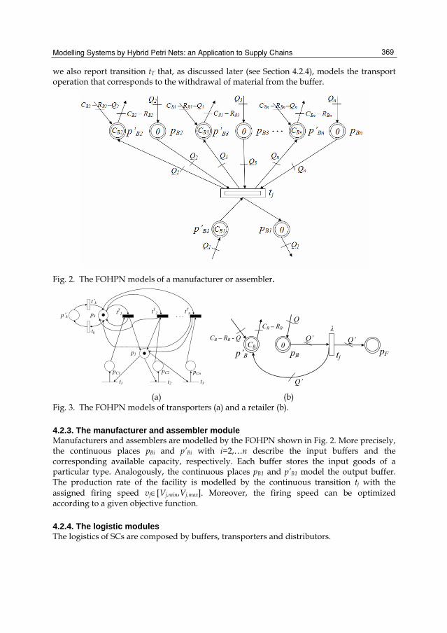
we also report transition tT that, as discussed later (see Section 4.2.4), models the transport operation that corresponds to the withdrawal of material from the buffer.

Fig. 2. The FOHPN models of a manufacturer or assembler.

p’k pk

t’k

tk

tT1

pC1

. . .

pC2 pCn

tTn

t1 t2 t3

tT2

p1 pB p’B tj pF

Q

CB – RB - Q

CB – RB

CB 0

Q’

Q’ Q’ λ

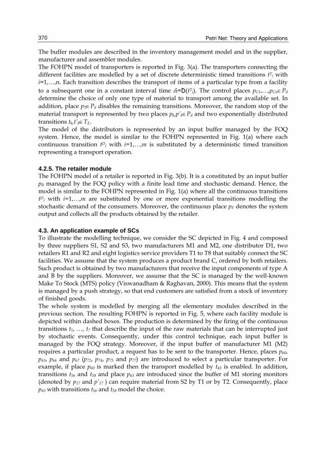
(a) (b)

Fig. 3. The FOHPN models of transporters (a) and a retailer (b).

4.2.3. The manufacturer and assembler module Manufacturers and assemblers are modelled by the FOHPN shown in Fig. 2. More precisely, the continuous places pBi and p’Bi with i=2,…n describe the input buffers and the corresponding available capacity, respectively. Each buffer stores the input goods of a particular type. Analogously, the continuous places pB1 and p’B1 model the output buffer. The production rate of the facility is modelled by the continuous transition tj with the assigned firing speed vj∈[Vj,min,Vj,max]. Moreover, the firing speed can be optimized according to a given objective function.

4.2.4. The logistic modules The logistics of SCs are composed by buffers, transporters and distributors.


The buffer modules are described in the inventory management model and in the supplier, manufacturer and assembler modules. The FOHPN model of transporters is reported in Fig. 3(a). The transporters connecting the different facilities are modelled by a set of discrete deterministic timed transitions tTi with i=1,…,n. Each transition describes the transport of items of a particular type from a facility to a subsequent one in a constant interval time δi=D(tTi). The control places pC1,…,pCn∈Pd determine the choice of only one type of material to transport among the available set. In addition, place p1∈Pd disables the remaining transitions. Moreover, the random stop of the material transport is represented by two places pk,p’k∈Pd and two exponentially distributed transitions tk,t’k∈TE. The model of the distributors is represented by an input buffer managed by the FOQ system. Hence, the model is similar to the FOHPN represented in Fig. 1(a) where each continuous transition tDi with i=1,…,m is substituted by a deterministic timed transition representing a transport operation.

4.2.5. The retailer module The FOHPN model of a retailer is reported in Fig. 3(b). It is a constituted by an input buffer pB managed by the FOQ policy with a finite lead time and stochastic demand. Hence, the model is similar to the FOHPN represented in Fig. 1(a) where all the continuous transitions tDi with i=1,…,m are substituted by one or more exponential transitions modelling the stochastic demand of the consumers. Moreover, the continuous place pF denotes the system output and collects all the products obtained by the retailer.

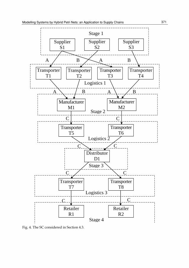
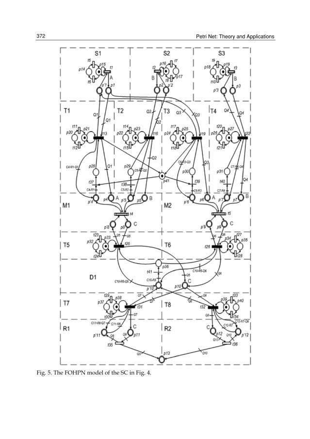
4.3. An application example of SCs To illustrate the modelling technique, we consider the SC depicted in Fig. 4 and composed by three suppliers S1, S2 and S3, two manufacturers M1 and M2, one distributor D1, two retailers R1 and R2 and eight logistics service providers T1 to T8 that suitably connect the SC facilities. We assume that the system produces a product brand C, ordered by both retailers. Such product is obtained by two manufacturers that receive the input components of type A and B by the suppliers. Moreover, we assume that the SC is managed by the well-known Make To Stock (MTS) policy (Viswanadham & Raghavan, 2000). This means that the system is managed by a push strategy, so that end customers are satisfied from a stock of inventory of finished goods. The whole system is modelled by merging all the elementary modules described in the previous section. The resulting FOHPN is reported in Fig. 5, where each facility module is depicted within dashed boxes. The production is determined by the firing of the continuous transitions t1, …, t7 that describe the input of the raw materials that can be interrupted just by stochastic events. Consequently, under this control technique, each input buffer is managed by the FOQ strategy. Moreover, if the input buffer of manufacturer M1 (M2) requires a particular product, a request has to be sent to the transporter. Hence, places p60, p63, p66 and p67 (p72, p74, p75 and p77) are introduced to select a particular transporter. For example, if place p60 is marked then the transport modelled by t43 is enabled. In addition, transitions t56 and t58 and place p63 are introduced since the buffer of M1 storing monitors (denoted by p17 and p’17 ) can require material from S2 by T1 or by T2. Consequently, place p63 with transitions t56 and t58 model the choice.


Logistics 2

Stage 2

Stage 4

Logistics 3

Supplier S1

Supplier S2

TransporterT2

Transporter T3

Manufacturer M1

Manufacturer M2

Transporter T5

Transporter T6

B A

C

Stage 3

DistributorD1

TransporterT7

Transporter T8

Retailer R1

Retailer R2

Supplier S3

TransporterT1

Transporter T4

A B

Stage 1

Logistics 1

A B A B

C

C C

C C

C C

Fig. 4. The SC considered in Section 4.3.


Fig. 5. The FOHPN model of the SC in Fig. 4.


4.3.1. Simulation and optimization The SC dynamics is analyzed via numerical simulation using the data reported in Table 1, where we can read the manufacturer production rates range, the range of transportation speeds and the average firing delays of discrete stochastic transitions. Table 2 shows further data necessary to completely describe the system, namely the initial markings of continuous places, the buffer capacities for the inventories of each stage and the values of the reorder levels and fixed order quantities. In order to analyze the SC behavior, some basic performance indices are assumed (Gershwin, 2002, Viswanadham, 2000): 1. the system throughput T, i.e., the average number of products obtained by the retailers

in a time unit; 2. the average system inventory SI, i.e., the average amount of products stored in all the

system input buffers during the run time TP; 3. the lead time LT=SI/T that is a measure of the time spent by the SC in converting the

raw material into final products. The FOHPN model has been implemented and simulated in the well-known Matlab environment (The Mathworks, 2006). Indeed, such a matrix-based software appears particularly appropriate for simulating the FOHPN dynamics based on the matrix formulation of the marking update described in Section 3. In particular, the chosen software program is able to integrate modelling and simulation of hybrid systems with the solution of constrained optimization problems, i.e., the IFS vector choice within the set of admissible values by optimizing a particular objective function. In more detail, after defining the system parameters and the initial marking, the main simulation program first selects the value of each transition timer set point, then determines the set of IFS admissible vectors and solves the optimization program by a suitable Matlab routine; it subsequently determines the next macro-event to occur using an appropriate routine that singles out the enabled transitions. Hence, the simulation determines the next marking with the matrix formulation of the marking update described in Section 3, and finally updates the set point of all transitions so that the next macro-period may be simulated. All the indices assessing the performance of the SC dynamics are estimated by simulation runs of a time period TP=480 hours and 1000 independent replications. Moreover, the simulations are performed in two operative conditions, denoted OCi with i=1,2 and each operative condition OCi corresponds to a different choice of the IFS vectors within the set of admissible values. • First Operative Condition (OC1). At each macro-period the IFS vector v is selected so as to

maximize the sum of all flow rates (see first item in Section 3.5) • Second Operative Condition (OC2). At each macro-period the IFS vector v is selected so as

to minimize the stored volume (see third item in Section 3.5) The main results of the numerical simulations we carried out are summarized in Table 3. In particular, OC1 provides the best performances in terms of system throughput. This result is not surprising because in such operational condition the goal was exactly that of maximizing the sum of all flow rates. Moreover, Table 3 shows the average inventories in the two operative conditions. The values show that the SC is able to keep stocks at a satisfactorily high level, so that the demand is satisfied and inventory is not excessive. In particular, as expected, OC1 corresponds to the highest inventories and OC2 to the lowest


stocks. Finally, Table 3 reports the obtained lead times in the two conditions, showing that the obtained LT values in OC1 are greater than those obtained in OC2, since the former case corresponds to a higher productivity. Summing up, a different choice of the production and work rates (as in the two cases OC1 and OC2) lets us manage the different performance indices of the SC, i.e. the system may forced to evolve in an optimal way, e.g. while maximizing the flow rates or minimizing the inventory.

Continuous transitions Discrete transitions

[Vmin, Vmax] Exponential

Average firing delay

(hours) Timed

Firing delay

(hours)

t1 t5 t7 [2, 4] t22 t40 2 t53 1 t2 t3 t4 [3, 5] t16 t26 t34 3 t42 t43 2

t6 [4, 6] t10 t14 t18 4 t47 t48 2 t8 [0,7] t24 t28 t32 4 t52 t54 2 t9 [0,6] t36 t38 4 t44 t45 3 t20 t30 t41 5 t46 t49 3 t12 6 t50 t51 3 t13 18 t21 t31 19 t11 t15 t19 20 t25 t29 t33 20 t37 t39 20 t17 t27 t35 21 t23 22

Table 1: Firing speeds and average firing delay of continuous and discrete transitions

Initial markings Product units Capacities Reorder levels Fixed Order

quantities m1 m5 m11 m15 20 C1,C5,C11,C15=100 R1=18 Q1,Q6=50

m23 m25 20 C23,C25=100 R2,R3,R4=25 Q2=45 m31 m37 m39 20 C31 =150 C37,C39=70 R5,R6=15 Q3=55 m3 m9 m13 15 C3,C9,C13=100 R7,R8=20 Q4=40

m7 m27 25 C7,C27=100 R9=30 Q5=60 m17 m19 m29 30 C17,C19,C29=100 R10,R11=10 Q7=30

m33 30 C33=150 Q8=25 m21 35 C21=100 Q9=2

m35 m41 0 C35=120 Q10=5 Table 2: Initial marking of odd continuous places, capacities and edge weights.

OC1 OC2 T

units/h SI

units LT

hours T

units/h SI

units LT

hours 2.04 1203 589 1.92 817 425

Table 3: The performance indices.


5. Conclusion In this paper we focused our attention on a particular hybrid PN model called FOHPN, that is based on the fluidification of discrete PNs, and whose main feature is that the instantaneous firing speed of continuous transitions keeps constant during each macro-period. In the first part of the paper we discuss in detail the advantages of fluidification, and provide a brief survey of the most important formalisms within the hybrid PN framework. Finally, we showed how FOHPNs can be efficiently used to model SC, and how interesting optimization problems can be solved via numerical simulation, by simply solving on-line a certain number of LPPs.

6. References Ajmone Marsan, M., Balbo, G., Conte, G., Donatelli, S., Franceschinis, G. (1995). Modelling

with Generalized Stochastic Petri Nets, John Wiley & sons, 1995. Alla, H. & David, R. (1998). “A modeling and analysis tool for discrete events systems:

continuous Petri Nets”, Performance Evaluation, Vol. 33, No. 3, pp. 175-199. Alur, R., Courcoubetis, C., Henzinger, T.A. & Ho, P.H. (1993). “Hybrid Automata: an

Algorithmic Approach to the Specification and Verification of Hybrid Systems“, Lecture Notes in Computer Science, Springer Verlag, Vol. 736, pp. 209-229.

Amer-Yahia, C., Zerhouni, N., Ferney, M. & El Moudni, A. (1997). “Modelling of Biological Systems by Continuous Petri Nets”, Proc. 3rd IFAC Symp. Modelling and Control in Biomedical Systems, Warwick, UK.

Amer-Yahia, C. & Zerhouni, N. (2001). “ State equation and Stability for a Class of Continuous Petri Nets. Application to the Control of a Production System”, Studies in Informatics and Control, Vol. 10, No. 4, pp. 301-317.

Andreu, D., Pascal, J.C. & Valette, R. (1996). “Events as a key of a batch process control system”, Proc. CESA'96, Symp. On Discrete Events and Manufacturing Systems, Lille, France, 1996.

Balduzzi, F., Giua, A. & Seatzu, C. (2001). “Modelling and Simulation of Manufacturing Systems Using First-Order Hybrid Petri Nets”, Int. J. of Production Research, Vol. 39, No. 2, pp. 255-282.

Balduzzi, F., Giua, A. & Menga, G. (2000). “First-Order Hybrid Petri Nets: a Model for Optimization and Control”, IEEE Trans. Robotics and Automation, Vol. 16, pp. 382-399.

Beamon, B.M. (1999). “Measuring Supply Chain Performance”, International Journal of Operations and Production Management, vol. 19, pp. 257-292, 1999.

Bemporad, A., Júlvez, J., Recalde, L., Silva, M. (2004). “Event-driven optimal control of continuous Petri nets”, Proc. 43th IEEE Conf. on Decision and Control, Atlantis, Paradise Island, Bahamas.

Champagnat, R., Esteban, P., Pingaud, H. & Valette, R. (1998). “Modeling and Simulation of a Hybrid System Through PR/TR PN-DAE Model, Proc. 3rd Int. Conf. on Automation of Mixed Processes, Reims, France.

Chen, H. & Hanisch, H.-M. (1998). “Hybrid net condition/event systems for modeling and analysis of batch processes“, Proc. 3rd Int. Conf. on Automation of Mixed Processes, Reims, France.


Chen, H., Amodeo, L., Chu, F. & Labadi, K. (2005). “Modeling and performance evaluation of supply chains using batch deterministic and stochastic Petri nets”, IEEE Transactions on Automation Science and Engineering, vol. 2, no. 2, pp. 132-144.

David, R. & Alla, H. (1987). “Continuous Petri Nets", Proc. 8th European Workshop on Application and Theory of Petri Nets, Zaragoza, Spain.

David, R. & Alla, H. (2005). Discrete, continous and hybrid Petri nets, Springer, Berlin, Heidelberg.

Demongodin, I. & Koussoulas, N.T. (1998). “Differential Petri Nets: Representing Continuous Systems in a Discrete-Event World”, IEEE Trans. on Automatic Control, Vol. 43, No. 4, pp. 573-579.

Demongodin, I., Caradec, M. & Prunet, F., (1998). “Fundamental Concepts of Analysis in Batches Petri Nets”, Proc. 1998 IEEE Int. Conf. on Systems, Man, and Cybernetics, San Diego, CA,USA.

Demongodin, I. & Giua, A. (2002). “Some analysis methods for continuous and hybrid Petri nets”, Proc. IFAC World Congress, Barcelona, Spain

Desrochers, A., Deal, T.J. & Fanti, M.P. (2005). “Complex-Valued Token Petri nets”, IEEE Transactions on Automation Science and Engineering, vol. 2, no. 4, pp. 309-318.

Dubois, E., Alla, H. & David, R. (1994). “Continuous Petri Net with Maximal Speeds Depending on Time”, Proc. 15th Int. Conf. on Application and Theory of Petri Nets", Zaragoza, Spain.

Dotoli, M., Fanti, M.P., Giua, A. & Seatzu, C. (2007). “First-order hybrid Petri nets. An application to distributed manufacturing systems”, Nonlinear Analysis. Hybrid Systems, in press.

Dotoli, M., Fanti, M.P., Meloni, C., & Zhou, M.C. (2005). “A Multi-Level Approach for Network Design of Integrated Supply Chains”, International Journal of Production Research, vol. 43, no. 20, pp. 4267-4287.

Dotoli, M., Fanti, M.P., Meloni, C. & Zhou, M.C. (2006). “Design and Optimization of Integrated E-Supply Chain for Agile and Environmentally Conscious Manufacturing”, IEEE Transactions on Systems Man and Cybernetics, part A, Vol. 36, No. 1, pp. 62-75.

Flaus, J.-M. (1997). “Hybrid Flow Nets for Batch Process Modeling and Simulation”, Proc. 2nd IMACS Symp. On Mathematical Modeling, Vienna, Austria.

Flaus, J.-M. & Alla, H. (1997). “ Structural analysis of hybrid systems modelled by hybrid flow nets“, Proc. European Control Conference, Brussels, Belgium.

Furcas, R., Giua, A., Piccaluga, A. & Seatzu, C. (2001). “Hybrid Petri net modelling of inventory management systems”, European Journal of Automation APII-JESA, vol. 35, no. 4, pp. 417-434.

Gaujal, B. & Giua, A. (2004). “Optimal stationary behavior for a class of timed continuous Petri nets”, Automatica, vol. 40, no. 9, pp. 1505--1516.

Genrich, H.J. & Schuart, I. (1998). “Modeling and verification of hybrid systems using hierarchical coloured Petri Nets, Proc. 3rd Int. Conf. on Automation of Mixed Processes, Reims, France.

Gershwin S.B. (2002). “Manufacturing Systems Engineering”, Copyright S. Gershwin, Cambridge, MA, USA.

Giua, A. Pilloni, M.T., & Seatzu, C. (2005). “Modeling and simulation of a bottling plant using hybrid Petri nets”, Int. J. of Production Research, vol. 43, no. 7, pp. 1375-1395.


Giua, A. & Usai, E. (1998). “Modeling hybrid systems by high-level Petri nets”, European Journal of Automation APII-JESA, vol. 32, no. 9-10, pp. 1209-1231.

Júlvez, J., & Boel R. (2005). “Modelling and controlling traffic behaviour with continuous Petri nets”, Proc. 16th IFAC World Congress, Prague, Czech Republic.

Júlvez, J., Recalde, L. & Silva, M. (2002). “On deadlock-freeness analysis of autonomous and timed continuous mono-T semiflow nets”, Proc. 41th IEEE Conf. on Decision and Control, Las Vegas, USA.

Júlvez, J., Recalde, L. & Silva, M. (2003). “On reachability in autonomous continuous {P}etri net systems“, Lecture Notes in Computer Science, Springer Verlag, vol. 2679, pp. 221-240.

Júlvez, J., Jimènez, E., Recalde, L. & Silva, M. (2004). “Design of observers for timed CPN systems“, Proc. IEEE Int. Conf. on Systems, Man, and Cybernetics, The Hague, The Netherlands.

Lefebvre, D. (2000). “Estimation of the production frequencies for manufacturing systems”, IMA J. of Management Mathematics, vol. 11, no. 4.

Mahulea, C., Giua, A., Recalde, L., Seatzu, C. & M. Silva, M., (2006a). “Optimal control of timed continuous Petri nets via explicit MPC”, Lecture Notes in Computer Science, Springer Verlag, vol. 341, pp. 383-390.

Mahulea, C., Recalde, L. & M. Silva, M. (2006b). “On performance monotonicity and basic servers semantics of continuous Petri nets”, 8th Int. Workshop on Discrete Event Systems, Michigan, USA.

Mahulea, C., Ramirez Treviño, A., Recalde, L., & Silva, M. (2007). “Steady state control reference and token conservation laws in continuous Petri net systems”, IEEE Trans. on Automation Science and Engineering, in press.

Murata, T. (1989). “Petri Nets: Properties, Analysis and Applications”, Proceedings IEEE, vol. 77, pp. 541-580.

Petri, C.A. (1962). “Kommunikation mit Automaten (Communication with automata)”, Ph.D. Thesis.

Puri, A. & Varaiya, P. (1996). “Decidable Hybrid Systems“, Computer and Mathematical Modeling, vol. 23, no. 11-12, pp. 191-202.

Silva, M., Teruel, E., & Colom, J. M. (1996). “Linear algebraic and linear programming techniques for the analysis of net systems”, Lectures on Petri Nets I: Basic Models, Advances in Petri Nets, Lecture notes in Computer Science, vol. 1491, pp. 309-373, Springer.

The MathWorks Inc., Matlab Release Notes For Release 14. Natick, MA, 2006. Trivedi, K.S. & Kulkarni, V.G. (1993). “FSPNs: Fluid Stochastic Petri Nets”, Lecture Notes in

Computer Science, Springer Verlag, vol. 691, pp. 24-31. Valentin-Roubinet, C. (1998). “Modeling of hybrid systems: DAE supervised by Petri Nets.

The example of a gas storage”, Proc. 3rd Int. Conf. on Automation of Mixed Processes, Reims, France.

Viswanadham, N. (2000). “Analysis of manufacturing enterprises”, Kluwer Academic Publishers, Boston, MA, USA.

Viswanadham, N. & Gaonkar, R.S. (2003).“Partner Selection and Synchronized Planning in Dynamic Manufacturing Networks”, IEEE Transactions on Robotics and Automation, vol. 19, no. 1, pp. 117-130.


Viswanadham, N. & Raghavan, S. (2000). “Performance Analysis and Design of Supply Chains: a Petri Net Approach”, Journal of the Operational Research Society, vol. 51, pp. 1158-1169.

Vollmann, T.E., Berry, W.L., Whybark, D.C. & Jacobs, F.R., Manufacturing Planning and Control Systems for Supply Chain Management, Irwin/Mc Graw Hill, New York, 2004.

Zhou, M.C. & Venkatesh, K. (1998). “Modeling, Simulation and Control of Flexible Manufacturing Systems. A Petri Net Approach”, World Scientific, Singapore.

modelling systems by hybrid petri nets: an application … · · 2008-01-10modelling systems by...

Documents