modelling of a vector-controlled
DESCRIPTION
Modelling of a vector-controlledTRANSCRIPT
Noelia Hurtado López-Plaza
Modelling of a vector-controlledbearingless synchronous reluctance motordrive
School of Electrical Engineering
Espoo September 10, 2014
Project supervisor:
Prof. Marko Hinkkanen
aalto universityschool of electrical engineering
abstract ofthe final
project
Author: Noelia Hurtado López-Plaza
Title: Modelling of a vector-controlled bearingless synchronous reluctancemotor drive
Date: September 10, 2014 Language: English Number of pages:9+47
Department of Electrical Engineering and Automation
Professorship: Electric Drives Code: S-81
Supervisor and instructor: Prof. Marko Hinkkanen
This final project deals with the modelling of a vector-controlled bearingless syn-chronous reluctance motor (BSyRM) drive. The goal of this project is to developthe dynamic model of a BSyRM. A brief introduction going through the advantagesand disadvantages of conventional machines shows the importance of BSyRMs de-velopment. An explanation about the general aspects and operating principles ofBSyRMs is presented together with the general dynamic model equations of thepermanent-magnets synchronous machine. Several assumptions are considered toadapt the permanent-magnets machine model to the BSyRM model desired. Thedescription of the controllers employed in the vector control implementation isalso included. The study is made through a literature review and by simulationusing the Matlab/Simulink software. The implementation of the BSyRM dynamicmodel and vector control and the simulation results are presented. Simulationsshow that the model developed is well suited for the BSyRM.
Keywords: Bearingless synchronous reluctance motor, motor windings, suspen-sion windings, radial force, vector control
aalto universityschool of electrical engineering
Abstract delProyecto Fin
de Carrera
Autor: Noelia Hurtado López-Plaza
Título: Modelado de un motor síncrono de reluctancia sin rodamientoscontrolado vectorialmente
Fecha: September 10, 2014 Idioma: Inglés Número de páginas:9+47
Departamento de Ingeniería Eléctrica y Automática
Cátedra: Vehículos Eléctricos Código: S-81
Tutor: Prof. Marko Hinkkanen
Este proyecto final de carrera aborda el modelado de un motor síncrono de reluc-tancia sin rodamientos controlado vectorialmente. El objetivo del proyecto es eldesarrollo del modelo dinámico del motor síncrono de reluctancia sin rodamientos.Una breve introducción repasando las ventajas e inconvenientes de los motores con-vencionales, nos muestra la importancia del desarrollo de motores sin rodamientos.El proyecto incluye la definición de los aspectos más generales y principios de fun-cionamiento de este tipo de motores, junto con las ecuaciones generales del modelodinámico del motor síncrono de imanes permanentes. Distintas suposiciones sonllevadas a cabo para adaptar las ecuaciones del modelo de imanes permanentes almodelo síncrono de reluctancia sin rodamientos deseado. La descripción detalladadel control vectorial empleado en la realización del proyecto también se incluye. Elestudio se ha llevado a cabo mediante la revisión de la literatura previa referenteal tema y de varias simulaciones en el entorno Matlab/Simulink. La construccióndel modelo dinámico y del control vectorial del motor junto con los resultados delas simulaciones, son incluidos en el proyecto. Los resultados que se presentanmuestran como el modelo desarrolado es adecuado para los motores síncronos dereluctancia sin rodamientos.
Palabras clave: Motor síncrono de reluctancia sin rodamientos, bobinados delmotor, bobinados de la suspensión, fuerza radial, control vecto-rial
iv
PrefaceThe work of this Final Project was done in the Electric Drives group, on the De-partment of Electrical Engineering and Automation at the School of Electrical Engi-neering of the Aalto University, in Helsinki, Finland. The group is led by ProfessorMarko Hinkkanen.
I am very grateful to my supervisor Prof. Marko Hinkkanen, for giving me theopportunity of joining this project and trust me. His support and advices in ourlong meetings have been very important to keep on working every day with illusion.
I would also like to express my gratitude to my office mates, specially Jarno,Jussi and Elahe. You were always willing to help me with any problem I had.
A special mention to my Erasmus family, thank you for all the moments we havelived together, without all of you this experience would have never been the same.A very special mention to my “Gorditos”, Nicola and Alberto, thank you for beingas you are and for all the funny/crazy moments full of laughter and for others fullof tears, you know this is just the beginning of our adventure.
Alicia and Coco, my dear flatmates, with whom I have been living almost oneyear, I could not have been luckier, you are the best company anybody can have.Thank you cutie for taking care of me and being my confident, for all the momentswe shared, our travels, parties and deep conversations in the early morning.
Bea, with whom I spent the best and worse moments of the degree at ETSIIM.After too many hours studying at university, now we can say we have achieved it,we are engineers!. I am also very grateful to the UPM for giving me the chance tocome to Finland and improve as person and as engineer.
Finally, my deepest appreciation goes to my family, for their endless supportduring all these years and for every time we share. To my mum, MaJosé, and tomy dad, Manuel, for being there for me in good and bad times always with wisewords, and to my brother, Jorge, that I am sure will become an important physi-cist. To Pirata for the happy moments he gave us and to Cala for making us smileagain. To my grandparents, Adela and Cipriano, for teaching me that there are stillgood persons in the world. And my last words to Gabri, for giving me these wonder-ful months and support me every day with a smile on his face, thank you "campeón".
“Do not be sad because it is over, be happy because it happened"
Otaniemi, September 9, 2014.
Noelia Hurtado López-Plaza
v
ContentsAbstract ii
Abstract (in Spanish) iii
Preface iv
Contents v
Symbols and abbreviations vii
1 Introduction 1
2 Bearingless synchronous reluctance motor drive 32.1 Bearingless synchronous reluctance motors . . . . . . . . . . . . . . . 3
2.1.1 General aspects . . . . . . . . . . . . . . . . . . . . . . . . . . 42.1.2 Mechanical structure . . . . . . . . . . . . . . . . . . . . . . . 62.1.3 Principles of radial force generation . . . . . . . . . . . . . . . 7
2.2 Space vectors . . . . . . . . . . . . . . . . . . . . . . . . . . . . . . . 92.3 Dynamic model equations . . . . . . . . . . . . . . . . . . . . . . . . 11
2.3.1 Voltage equations . . . . . . . . . . . . . . . . . . . . . . . . . 112.3.2 Flux equations . . . . . . . . . . . . . . . . . . . . . . . . . . 122.3.3 Torque and motion equations . . . . . . . . . . . . . . . . . . 132.3.4 Suspension force equations . . . . . . . . . . . . . . . . . . . . 13
2.4 Operating principle . . . . . . . . . . . . . . . . . . . . . . . . . . . . 142.5 Parameters and assumptions . . . . . . . . . . . . . . . . . . . . . . . 16
3 Vector control 183.1 Vector control theory in bearingless motors . . . . . . . . . . . . . . . 18
3.1.1 Motor control system . . . . . . . . . . . . . . . . . . . . . . . 183.1.2 Suspension control system . . . . . . . . . . . . . . . . . . . . 19
3.2 Assumptions . . . . . . . . . . . . . . . . . . . . . . . . . . . . . . . . 193.3 Current controller . . . . . . . . . . . . . . . . . . . . . . . . . . . . . 203.4 Decoupling controller . . . . . . . . . . . . . . . . . . . . . . . . . . . 233.5 Parameters . . . . . . . . . . . . . . . . . . . . . . . . . . . . . . . . 24
4 Simulink model 254.1 Machine model . . . . . . . . . . . . . . . . . . . . . . . . . . . . . . 25
4.1.1 Voltage equations block . . . . . . . . . . . . . . . . . . . . . 274.1.2 Flux equations block . . . . . . . . . . . . . . . . . . . . . . . 274.1.3 Torque and motion equations blocks . . . . . . . . . . . . . . 284.1.4 Force equations block . . . . . . . . . . . . . . . . . . . . . . . 28
4.2 Vector control model . . . . . . . . . . . . . . . . . . . . . . . . . . . 284.2.1 Angular speed controller . . . . . . . . . . . . . . . . . . . . . 294.2.2 Motor decoupling . . . . . . . . . . . . . . . . . . . . . . . . . 294.2.3 Suspension decoupling . . . . . . . . . . . . . . . . . . . . . . 29
vi
4.2.4 Motor current controller . . . . . . . . . . . . . . . . . . . . . 314.2.5 Suspension current controller . . . . . . . . . . . . . . . . . . 31
5 Simulation results 335.1 Case 1 . . . . . . . . . . . . . . . . . . . . . . . . . . . . . . . . . . . 345.2 Case 2 . . . . . . . . . . . . . . . . . . . . . . . . . . . . . . . . . . . 365.3 Case 3 . . . . . . . . . . . . . . . . . . . . . . . . . . . . . . . . . . . 36
6 Conclusions 39
References 40
A Appendix 42A.1 Simulink dynamic model . . . . . . . . . . . . . . . . . . . . . . . . . 42
A.1.1 Flux equations . . . . . . . . . . . . . . . . . . . . . . . . . . 43A.1.2 Torque equation . . . . . . . . . . . . . . . . . . . . . . . . . . 44A.1.3 Motion equation . . . . . . . . . . . . . . . . . . . . . . . . . 44
A.2 Simulink vector control model . . . . . . . . . . . . . . . . . . . . . . 45A.2.1 Angular speed controller . . . . . . . . . . . . . . . . . . . . . 46A.2.2 Motor decoupling . . . . . . . . . . . . . . . . . . . . . . . . . 46A.2.3 Suspension decoupling . . . . . . . . . . . . . . . . . . . . . . 47
vii
Symbols and abbreviations
Symbols
em Back-EMFF ij Radial force vector in rotating coordinatesFi Radial force i-axisFj Radial force j-axisF xy Radial force vector in stationary coordinatesFx Radial force x-axisFy Radial force y-axisFc Transfer function PI-controllerF c,m PI-type motor current controllerF c,s PI-type suspension current controllerGcc General closed-loop transfer functionGe General transfer functionGe,m Motor transfer function matrixGe,s Suspension transfer function matrixi Rotating reference i-axisi General current space vectorim Motor current space vectorima Motor current a-phaseimb Motor current b-phaseimd Motor current d-axisimq Motor current q-axisimu Motor current u-phaseimv Motor current v-phaseimw Motor current w-phaseis Suspension current space vectorisa Suspension current a-phaseisb Suspension current b-phaseisd Suspension current d-axisisq Suspension current q-axisisu Suspension current u-phaseisv Suspension current v-phaseisw Suspension current w-phaseI Identity matrixj Rotating reference j-axisJ Orthogonal rotation matrixJtot Moment of inertiaKi General integral gainKim Motor integral gain matrixKis Suspension integral gain matrixKp General proportional gain
viii
Kpm Motor proportional gain matrixKps Suspension proportional gain matrixL General inductanceL General inductance matrixLm Motor inductance matrixLd Motor d-axis inductanceLq Motor q-axis inductanceLs Suspension inductance matrixLs Suspension inductanceM Mutual inductance matrixM ′
d Suspension force constant d-axisM ′
q Suspension force constant q-axisp Pair of polesR General resistanceRm Motor resistanceRs Suspension resistanceTe Electromagnetic torqueTl Load torqueu General voltageu′ New general voltageum Motor voltage space vectorus Suspension voltage space vectorx Stationary reference x-axisy Stationary reference y-axisαc General current control bandwidthαcm Motor current control bandwidthαcs Suspension current control bandwidthαs Speed closed-loop system bandwidthθ Phase angle between current and terminal voltageτc General closed-loop electrical time constantφ Mechanical angle of the rotor between i- and x-axisφelec Electrical angle of the rotorψm Motor winding flux linkage space vectorψmd Motor flux linkage d-axis windingψmq Motor flux linkage q-axis windingψpm Permanent magnets flux linkage vectorψpm Permanent magnets flux linkageψ′pm Suspension force constant vectorψ′pm Suspension force constantψs Suspension winding flux linkage space vectorψsd Suspension flux linkage d-axis windingψsq Suspension flux linkage q-axis windingω Mechanical angular speed of the rotor
ix
Superscriptsxs Stator reference frame
Subscriptsref Reference value
Abbreviations
AC Alternating currentBSyRM Bearingless synchronous reluctance motorPI Proportional-integralPMSM Permanent-magnet synchronous motorSyRM Synchronous reluctance motor
1 Introduction
Synchronous reluctance motors (SyRMs) have recently become an interesting alter-native to other AC machines in variable-speed drives [1]. One of the main reasonsis that they drive well a very wide range of applications. Some of the characteristicsthat make modern transverse-laminated SyRMs so attractive are [2, 3]:
1. Simple and robust mechanical structure.
2. High efficiency and temperature capacity. The absence of the rotor windingresults in a higher efficiency and temperature capacity compared to the inductionmotor.
3. Low production cost. The absence of magnets in the rotor results in produc-tion savings compared to the permanent-magnet synchronous motor (PMSM)production.
4. Low vibration, noise and torque ripple. These magnitudes are lower in SyRMscompared to the switched reluctance motor.
5. High saliency ratio.
Although SyRMs have some advantages, there are still issues to be considered.One of the problems is the modelling of the magnetic saturation. Other importantproblem is that in high-speed applications, the losses of the mechanical bearingsbecome significant. Lubrication oil and bearings should be replaced periodically.In some environments, it is not easy to replace components, or the lubrication oilcannot be used. In order to avoid these losses, active magnetic bearings can be used,reducing the maintenance and removing the lubrication needs. However, there stillremain some problems in magnetic bearings. One of these problems is that magneticbearings require a large area. If the shaft length is increased to provide enough spaceto magnetic bearings, the critical rotating speed of the shaft decreases. To avoidcomplicated control of a flexible shaft, the length of the shaft has to be as short aspossible. [1, 4–9]
One of the solutions, to reduce the axial shaft length of high speed motors with mag-netic bearings, is to magnetically combine a motor with magnetic bearings. Hencebearingless synchronous reluctance motors (BSyRMs), are magnetically combinedelectric machines with magnetic bearings. Some of the most important advantagesdue to this integration are [1, 4–11]:
• Compactness. In BSyRMs the shaft length is shorter. Thus bearingless motorscan achieve higher speed than motors with conventional magnetic bearings,resulting in a more stable operation.
2
• High power. The length of the rotor can be effectively used to produce boththe torque and the radial magnetic force. Hence the electrical power requiredfor shaft levitation can be reduced because the magnetizing flux of the motoris utilized as a bias for the radial force generation.
• Low cost. The number of wires and inverters is lower.
Therefore BSyRM can be applied to many emerging applications, which requirea compact size, high-power, high reliability, long life, or wide temperature rangetogether with operation at high speeds or active vibration control.
Other types of bearingless motors, which have integrated magnetic bearings withelectric motors, have been proposed and developed actively in the last decades. Someof these motors are bearingless induction motors, bearingless switched reluctancemotors or bearingless permanent-magnet synchronous motors. These motors havebeen developed in order to fulfil the need of high-power and high-speed AC drivestogether with an enormous reduction in size and weight.
The machine used in this final project, is a BSyRM with 4-pole motor winding fortorque production, and 2-pole suspension winding for radial force generation. TheBSyRM is a special case of the PMSM. Therefore, general PMSM equations havebeen presented for the machine dynamic model, in order to study a more generalcase applicable to a wide range of machines [9]. These equations have been specifiedfor the BSyRM considering different assumptions.
The main goal of this final project is to describe the BSyRMs operation principles,to obtain the dynamic model equations and to implement the model of the machinein Simulink. An additional goal is to control the motor operation through the vectorcontrol developed. Hence, this final project will be focused in the development ofthe dynamic model and the vector control of BSyRMs.
In this final project, the description and operating principles of BSyRMs are ex-plained in Section 2. Subsequent the equations of the dynamic model are obtainedtogether with the assumptions and parameters used. The description of the vectorcontrol employed for controlling the machine is defined in Section 3. Section 4 in-cludes the implementation of both the machine model and the vector control modelof the BSyRM. Finally, Section 5 shows the simulations results obtained testing theMatlab/Simulink model developed, and Section 6 includes the final conclusions ofthis final project.
3
2 Bearingless synchronous reluctance motor drive
2.1 Bearingless synchronous reluctance motors
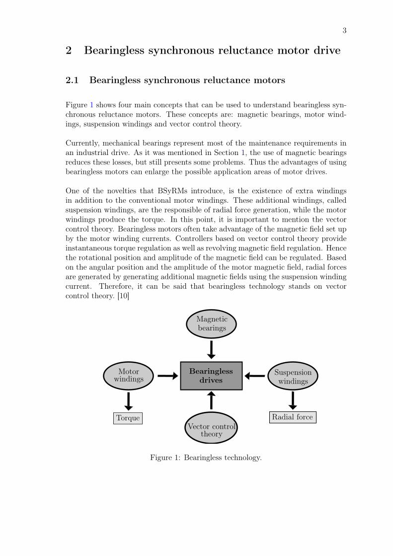
Figure 1 shows four main concepts that can be used to understand bearingless syn-chronous reluctance motors. These concepts are: magnetic bearings, motor wind-ings, suspension windings and vector control theory.
Currently, mechanical bearings represent most of the maintenance requirements inan industrial drive. As it was mentioned in Section 1, the use of magnetic bearingsreduces these losses, but still presents some problems. Thus the advantages of usingbearingless motors can enlarge the possible application areas of motor drives.
One of the novelties that BSyRMs introduce, is the existence of extra windingsin addition to the conventional motor windings. These additional windings, calledsuspension windings, are the responsible of radial force generation, while the motorwindings produce the torque. In this point, it is important to mention the vectorcontrol theory. Bearingless motors often take advantage of the magnetic field set upby the motor winding currents. Controllers based on vector control theory provideinstantaneous torque regulation as well as revolving magnetic field regulation. Hencethe rotational position and amplitude of the magnetic field can be regulated. Basedon the angular position and the amplitude of the motor magnetic field, radial forcesare generated by generating additional magnetic fields using the suspension windingcurrent. Therefore, it can be said that bearingless technology stands on vectorcontrol theory. [10]
Bearinglessdrives
Magneticbearings
Vector controltheory
Motorwindings
Suspensionwindings
Torque Radial force
Figure 1: Bearingless technology.

4
2.1.1 General aspects
The machine studied in this final project is a "4-pole and 2-pole winding" BSyRM.The 4-pole refers to the motor winding set for torque production, while the 2-polerefers to the suspension winding set for radial force generation.
Figure 2 shows the cross section of a 2-phase ac bearingless machine. Typically,both the rotor and the stator are constructed from laminated silicon steel. Thestator contains the slots for both n-pole motor windings and (n ± 2)-pole suspensionwindings. The 4-pole motor windings ma-mb and 2-pole suspension windings sa-sbcan be observed in Figure 2. The internal rotor has four salient poles and the field-winding conductors m are arranged so that 4-pole magnetization is produced. Twoperpendicular axes, x and y, are set to the stator according to the magnetizationdirection of the a-phase. The i- and j-axes are aligned on the magnetic poles. Thesei- and j-axes are fixed to the rotor so that they rotate with rotor rotation. Theradial position relationships between the i- and j-axes and the x- and y-axes aredefined by
[ij
]=
[cosφ sinφ− sinφ cosφ
] [xy
](1)
where the rotor angular position is defined by the angle φ. [10, 11]
Figure 2: 2-Phase ac bearingless machine. [10]
5
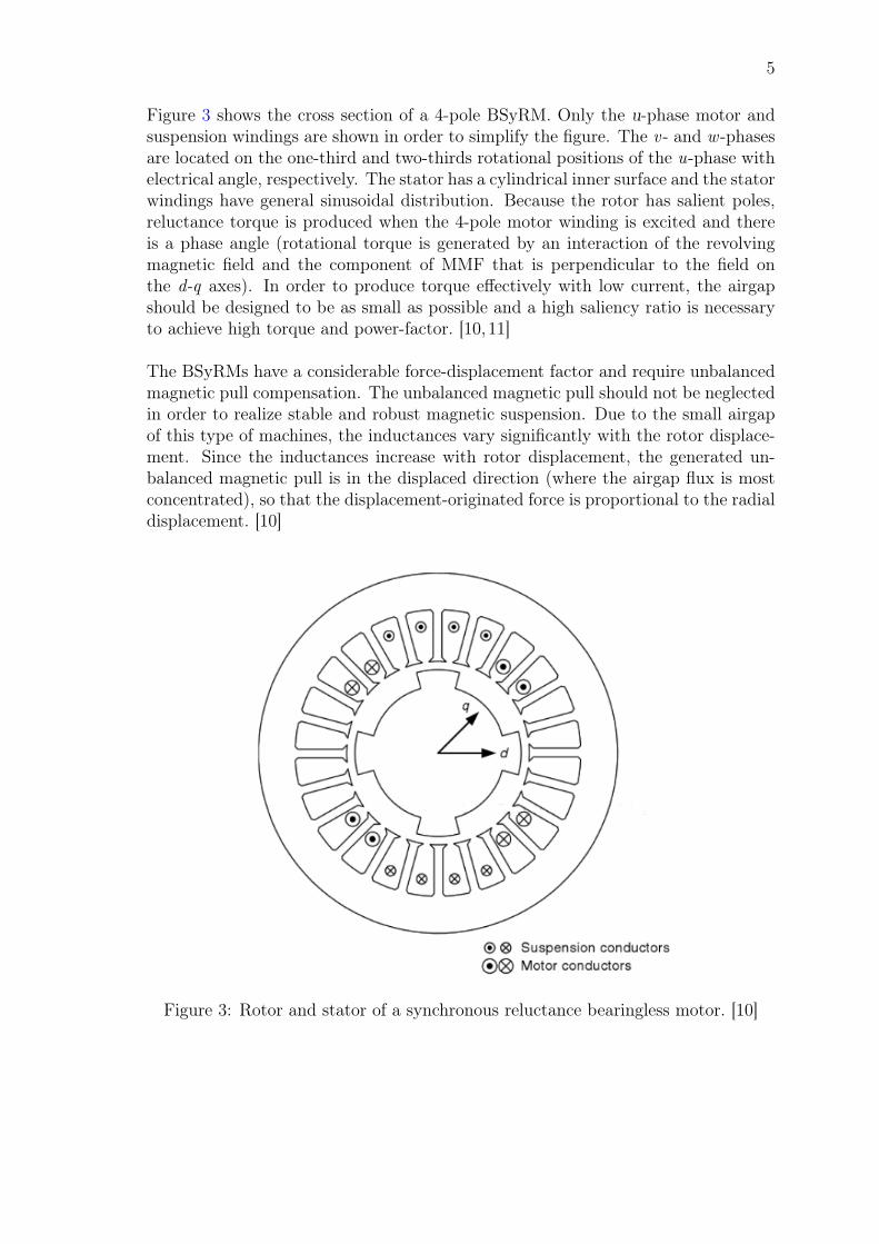
Figure 3 shows the cross section of a 4-pole BSyRM. Only the u-phase motor andsuspension windings are shown in order to simplify the figure. The v - and w -phasesare located on the one-third and two-thirds rotational positions of the u-phase withelectrical angle, respectively. The stator has a cylindrical inner surface and the statorwindings have general sinusoidal distribution. Because the rotor has salient poles,reluctance torque is produced when the 4-pole motor winding is excited and thereis a phase angle (rotational torque is generated by an interaction of the revolvingmagnetic field and the component of MMF that is perpendicular to the field onthe d-q axes). In order to produce torque effectively with low current, the airgapshould be designed to be as small as possible and a high saliency ratio is necessaryto achieve high torque and power-factor. [10,11]
The BSyRMs have a considerable force-displacement factor and require unbalancedmagnetic pull compensation. The unbalanced magnetic pull should not be neglectedin order to realize stable and robust magnetic suspension. Due to the small airgapof this type of machines, the inductances vary significantly with the rotor displace-ment. Since the inductances increase with rotor displacement, the generated un-balanced magnetic pull is in the displaced direction (where the airgap flux is mostconcentrated), so that the displacement-originated force is proportional to the radialdisplacement. [10]
Figure 3: Rotor and stator of a synchronous reluctance bearingless motor. [10]
6
2.1.2 Mechanical structure
Bearingless motors present several typical structures. Some of these structures aredescribed below. Other relevant structures can be found in the book written byChiba et al. [10]
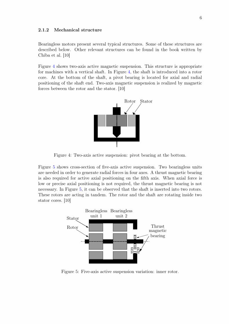
Figure 4 shows two-axis active magnetic suspension. This structure is appropriatefor machines with a vertical shaft. In Figure 4, the shaft is introduced into a rotorcore. At the bottom of the shaft, a pivot bearing is located for axial and radialpositioning of the shaft end. Two-axis magnetic suspension is realized by magneticforces between the rotor and the stator. [10]
StatorRotor
Figure 4: Two-axis active suspension: pivot bearing at the bottom.
Figure 5 shows cross-section of five-axis active suspension. Two bearingless unitsare needed in order to generate radial forces in four axes. A thrust magnetic bearingis also required for active axial positioning on the fifth axis. When axial force islow or precise axial positioning is not required, the thrust magnetic bearing is notnecessary. In Figure 5, it can be observed that the shaft is inserted into two rotors.These rotors are acting in tandem. The rotor and the shaft are rotating inside twostator cores. [10]
Stator
Rotor
Bearinglessunit 1
Thrustmagneticbearing
Bearinglessunit 2
Figure 5: Five-axis active suspension variation: inner rotor.
7
2.1.3 Principles of radial force generation
In both radial magnetic bearing and bearingless motors, rotor radial force is gener-ated by an unbalanced magnetic field; i.e., the rotor radial force is generated by thedifference of radial forces between the magnetic poles.
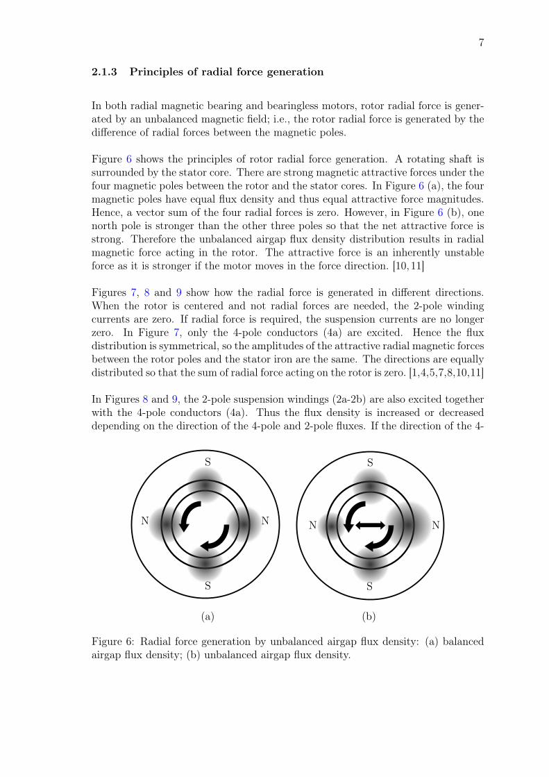
Figure 6 shows the principles of rotor radial force generation. A rotating shaft issurrounded by the stator core. There are strong magnetic attractive forces under thefour magnetic poles between the rotor and the stator cores. In Figure 6 (a), the fourmagnetic poles have equal flux density and thus equal attractive force magnitudes.Hence, a vector sum of the four radial forces is zero. However, in Figure 6 (b), onenorth pole is stronger than the other three poles so that the net attractive force isstrong. Therefore the unbalanced airgap flux density distribution results in radialmagnetic force acting in the rotor. The attractive force is an inherently unstableforce as it is stronger if the motor moves in the force direction. [10, 11]
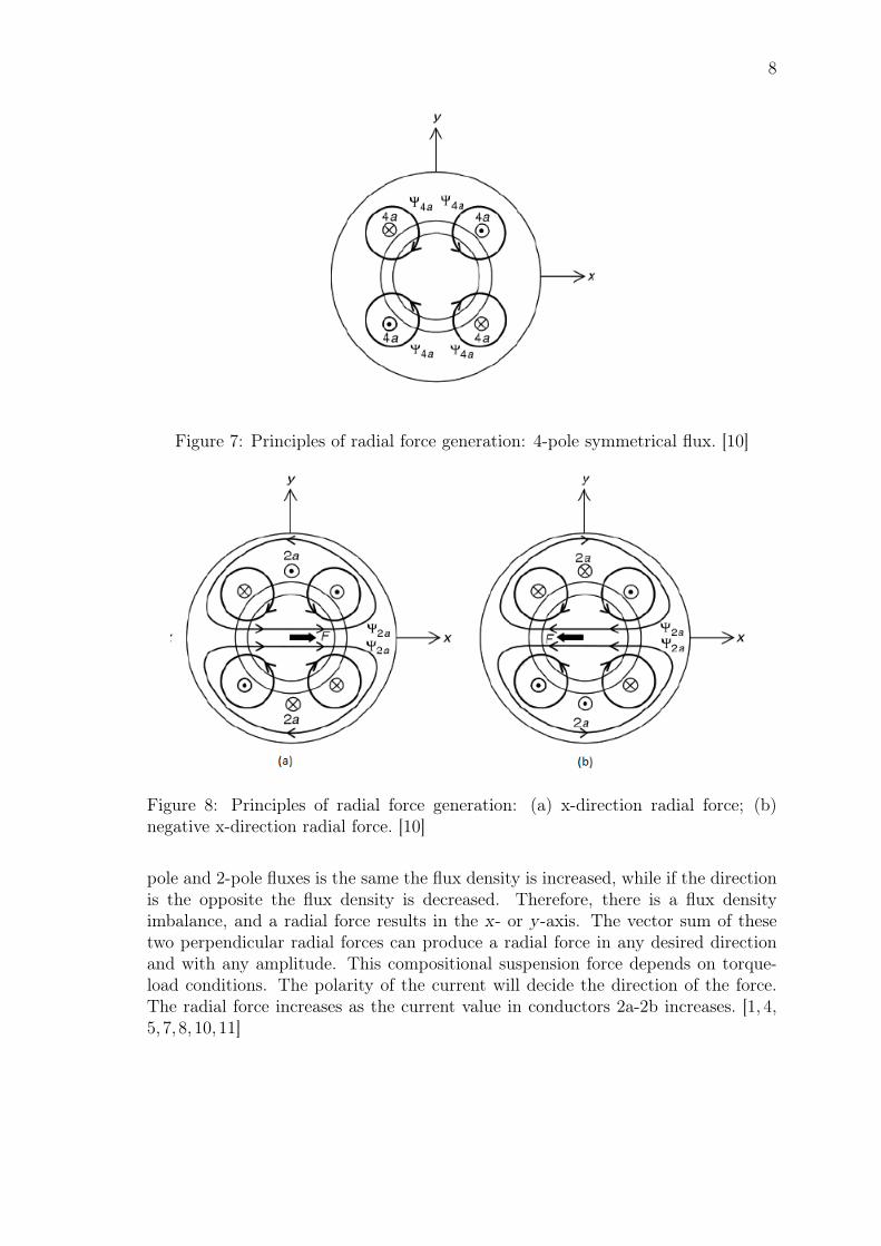
Figures 7, 8 and 9 show how the radial force is generated in different directions.When the rotor is centered and not radial forces are needed, the 2-pole windingcurrents are zero. If radial force is required, the suspension currents are no longerzero. In Figure 7, only the 4-pole conductors (4a) are excited. Hence the fluxdistribution is symmetrical, so the amplitudes of the attractive radial magnetic forcesbetween the rotor poles and the stator iron are the same. The directions are equallydistributed so that the sum of radial force acting on the rotor is zero. [1,4,5,7,8,10,11]
In Figures 8 and 9, the 2-pole suspension windings (2a-2b) are also excited togetherwith the 4-pole conductors (4a). Thus the flux density is increased or decreaseddepending on the direction of the 4-pole and 2-pole fluxes. If the direction of the 4-
S
N
S
S S
N N N
(a) (b)
Figure 6: Radial force generation by unbalanced airgap flux density: (a) balancedairgap flux density; (b) unbalanced airgap flux density.
8
Figure 7: Principles of radial force generation: 4-pole symmetrical flux. [10]
Figure 8: Principles of radial force generation: (a) x-direction radial force; (b)negative x-direction radial force. [10]
pole and 2-pole fluxes is the same the flux density is increased, while if the directionis the opposite the flux density is decreased. Therefore, there is a flux densityimbalance, and a radial force results in the x- or y-axis. The vector sum of thesetwo perpendicular radial forces can produce a radial force in any desired directionand with any amplitude. This compositional suspension force depends on torque-load conditions. The polarity of the current will decide the direction of the force.The radial force increases as the current value in conductors 2a-2b increases. [1, 4,5, 7, 8, 10,11]
9
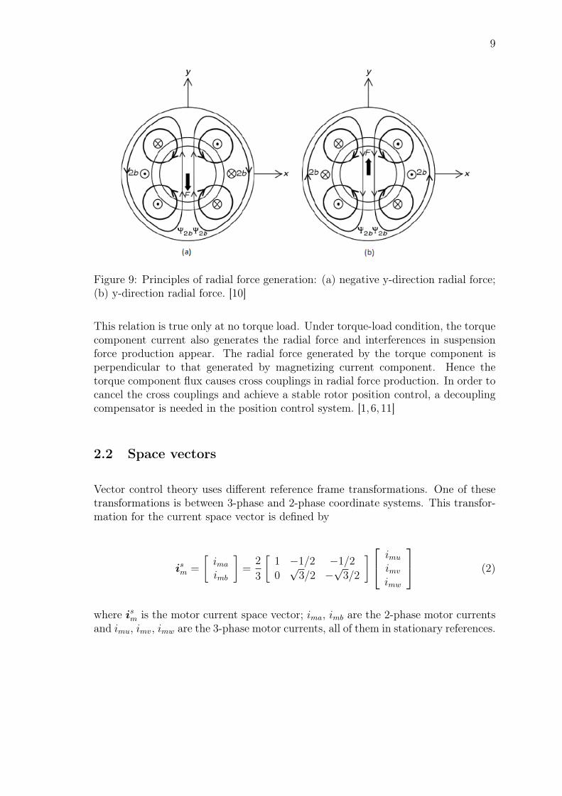
Figure 9: Principles of radial force generation: (a) negative y-direction radial force;(b) y-direction radial force. [10]
This relation is true only at no torque load. Under torque-load condition, the torquecomponent current also generates the radial force and interferences in suspensionforce production appear. The radial force generated by the torque component isperpendicular to that generated by magnetizing current component. Hence thetorque component flux causes cross couplings in radial force production. In order tocancel the cross couplings and achieve a stable rotor position control, a decouplingcompensator is needed in the position control system. [1, 6, 11]
2.2 Space vectors
Vector control theory uses different reference frame transformations. One of thesetransformations is between 3-phase and 2-phase coordinate systems. This transfor-mation for the current space vector is defined by
ism =
[imaimb
]=
2
3
[1 −1/2 −1/20√3/2 −
√3/2
] imuimvimw
(2)
where ism is the motor current space vector; ima, imb are the 2-phase motor currentsand imu, imv, imw are the 3-phase motor currents, all of them in stationary references.
10
A similar expression is shown for suspension windings
iss =
[isaisb
]=
2
3
[1 −1/2 −1/20√3/2 −
√3/2
] isuisvisw
(3)
where the suspension variables are analogous to the ones of the motor.
Another type of transformation is between stationary/rotating (ab/dq) referencesystems. This transformation applied to the motor current space vector can becarried out using the following matrix:
im =
[imdimq
]=
[cos 2φ sin 2φ− sin 2φ cos 2φ
] [imaimb
](4)
where im is the motor current space vector in rotating coordinates and imd, imq arethe 2-phase motor currents in rotating reference system (d - and q-axis). A similarexpression is used for suspension windings
is =
[isdisq
]=
[cosφ sinφ− sinφ cosφ
] [isaisb
](5)
It is necessary to distinguish between motor windings and suspension windings trans-formations, as the number of poles varies and therefore the angle used.
The motor and suspension windings transformations defined in the above expressions(4) and (5), can be also expressed using the following equations:
eJ2φ = cos (2φ)I + sin (2φ)J (6)
eJφ = cos (φ)I + sin (φ)J (7)
where the identity matrix and the orthogonal rotation matrix are defined as
I =
[1 00 1
]J =
[0 −11 0
]respectively.
11
2.3 Dynamic model equations
To implement the dynamic model of the bearingless synchronous reluctance machinethe following equations presented are needed. The equations are based on [8, 10,12]. These expressions will help to understand the operation and performance ofBSyRMs.
2.3.1 Voltage equations
The motor and suspension voltage equations in the stator reference frame (denotedby superscript s) are
dψsm
dt= usm −Rmi
sm (8)
dψss
dt= uss −Rsi
ss (9)
where ψm, ψs are the flux linkage space vectors; um, us are the voltage spacevectors; Rm, Rs are the resistances and im, is are the current space vectors of themotor and suspension windings, respectively, in each case.
In order to use rotating coordinates instead of stator coordinates, the followingtransformations are needed:
ψsm = ψme
J2φ (10)
ψss = ψse
Jφ (11)
The angular speed of the rotor is defined by
ω =dφ
dt(12)
where φ is the mechanical angle of the rotor between i -axis and x -axis as it wasmentioned previously.
12
Transforming (8) and (9) to the synchronous reference frame gives
dψm
dt= um −Rmim − J2ωψm (13)
dψs
dt= us −Rsis − Jωψs (14)
These expressions (13) and (14) will be used for the implementation of the voltageequations. The use of the equations in rotating coordinates is because if stationarycoordinates are employed, the flux equations would be much more complicated.
2.3.2 Flux equations
The relationships between flux linkage and winding currents can be expressed in amatrix form
ψmdψmqψsdψsq
=
Ld 0 M ′
di −M ′dj
0 Lq M ′qj M ′
qiM ′
di M ′qj Ls 0
−M ′dj M ′
qi 0 Ls
imdimqisdisq
+
ψpm0
ψ′pmi−ψ′pmj
(15)
where ψmd, ψmq, ψsd, ψsq and imd, imq, isd, isq are, respectively, flux linkages andcurrents of the motor and suspension d - and q-axis windings; Ld, Lq and Ls aremotor d - and q-axis inductances and suspension inductance; ψpm is the permanentmagnets flux linkage and ψ′pm (Wb/m),M ′
d (H/m) andM ′q (H/m) are the suspension
force constants.
The expression (15) can be also expressed in vector form
ψm = Lmim +Mis +ψpm (16)
ψs =MT im +Lsis +ψ
′pm (17)
where Lm, Ls are the motor and suspension inductance matrices, M is the mutualinductance matrix and ψpm and ψ′pm are the permanent magnets flux linkage andsuspension force constants vectors, respectively.
The definitions of the matrices mentioned above are
13
Lm =
[Ld 00 Lq
]Ls =
[Ls 00 Ls
]M =
[M ′
di −M ′dj
M ′qj M ′
qi
]
ψpm =
[ψpm0
]ψ′pm =
[ψ′pmi−ψ′pmj
]
2.3.3 Torque and motion equations
The electromagnetic torque of the bearingless synchronous reluctance machine canbe written as:
Te = 3[(Ld − Lq)imdimq + ψpmimq] (18)
The number 3 comes from 32p, where p is the number of pair of poles of the motor
windings. In the studied machine, p = 2. From (18) it is seen that the torque canbe controlled with both d-axis and q-axis motor winding currents.
The mechanical dynamics are governed by the equation of motion
dω
dt=
1
Jtot(Te − Tl) (19)
where Jtot is the moment of inertia and Tl is the load torque. The rotational speedof the shaft is controlled by the motor torque and described by (19). Mechanicaldynamics related to radial position are omitted in this final project.
2.3.4 Suspension force equations
The BSyRM produces a suspension force by the superposition of the 4-pole motorflux and the 2-pole suspension flux
[FiFj
]=
[M ′
dimd + ψ′pm M ′qimq
M ′qimq −M ′
dimd − ψ′pm
] [isdisq
](20)
The i- and j-axis suspension forces, Fi and Fj, are proportional to suspension cur-rents, isd and isq, and to coefficients M ′
dimd + ψ′pm and M ′qimq, as it is shown in the
14
equation (20). The variables ψ′pm, M ′dimd and M ′
qimq are the corresponding deriva-tives of the permanent magnets flux linkage and d- and q-axis winding flux linkageswith respect to the radial rotor displacement. Thus, suspension force characteristicsof bearingless motors can be determined using the suspension force constants ψ′pm,M ′
d and M ′q.
To modify the reference frame, some transformations should be completed
[FxFy
]=
[cosφ − sinφsinφ cosφ
] [FiFj
](21)
[isdisq
]=
[cosφ sinφ− sinφ cosφ
] [isaisb
](22)
where the subscripts x, y refer to stationary reference and i, j refer to rotatingreference system.
Applying the transformations (21) and (22) to the initial equation (20), it is obtained
[FxFy
]=
[M ′
dimd + ψ′pm −M ′qimq
M ′qimq M ′
dimd + ψ′pm
] [cos 2φ sin 2φsin 2φ − cos 2φ
] [isaisb
](23)
This matrix equation (23) shows the relationship between the suspension forces instationary coordinates as a function of the suspension winding currents. Thereforethe radial forces, Fx and Fy, can be regulated using the suspension currents isa andisb. The magnitude of the force is a function of the rotor angular position φ andthe suspension force constants which includes motor currents imd and imq. Thus thesuspension currents must be regulated in accordance with (23) in order to producethe required radial force.
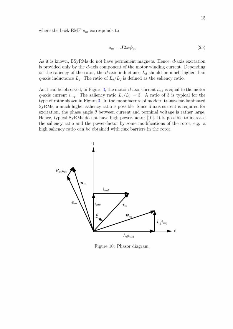
2.4 Operating principle
Figure 10 shows a SyRM phasor diagram. Different variables are represented in thefigure. The motor terminal voltage um comes from the steady state of the equation(13) and it is defined by
um = em +Rmim (24)
15
where the back-EMF em corresponds to
em = J2ωψm (25)
As it is known, BSyRMs do not have permanent magnets. Hence, d-axis excitationis provided only by the d-axis component of the motor winding current. Dependingon the saliency of the rotor, the d-axis inductance Ld should be much higher thanq-axis inductance Lq. The ratio of Ld/Lq is defined as the saliency ratio.
As it can be observed, in Figure 3, the motor d-axis current imd is equal to the motorq-axis current imq. The saliency ratio Ld/Lq = 3. A ratio of 3 is typical for thetype of rotor shown in Figure 3. In the manufacture of modern transverse-laminatedSyRMs, a much higher saliency ratio is possible. Since d-axis current is required forexcitation, the phase angle θ between current and terminal voltage is rather large.Hence, typical SyRMs do not have high power-factor [10]. It is possible to increasethe saliency ratio and the power-factor by some modifications of the rotor; e.g. ahigh saliency ratio can be obtained with flux barriers in the rotor.
q
d
imd
imq im
Rmim
em
um
Ldimd
Lqimq
θ ψm
Figure 10: Phasor diagram.
16
2.5 Parameters and assumptions
The choice of the BSyRM parameters used for testing the Simulink model, has beenbased on the book written by Chiba et al. [10] and on [6]. Different methods ofelectrical parameter identification are described on [13,14].
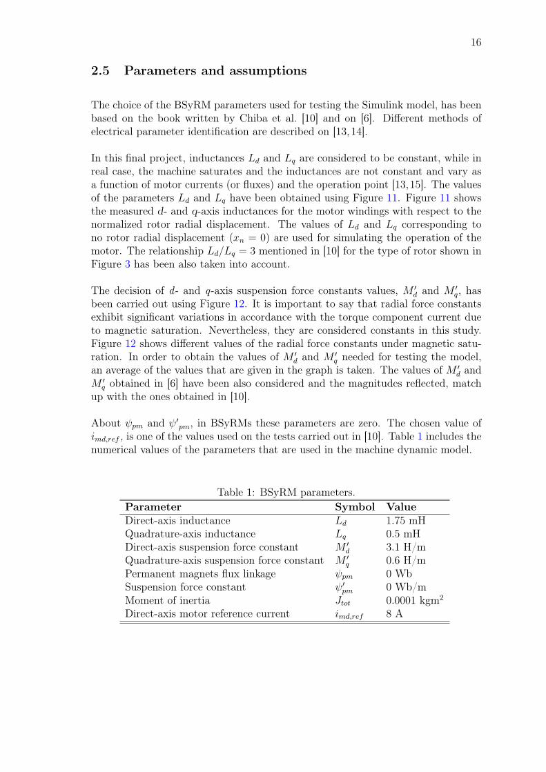
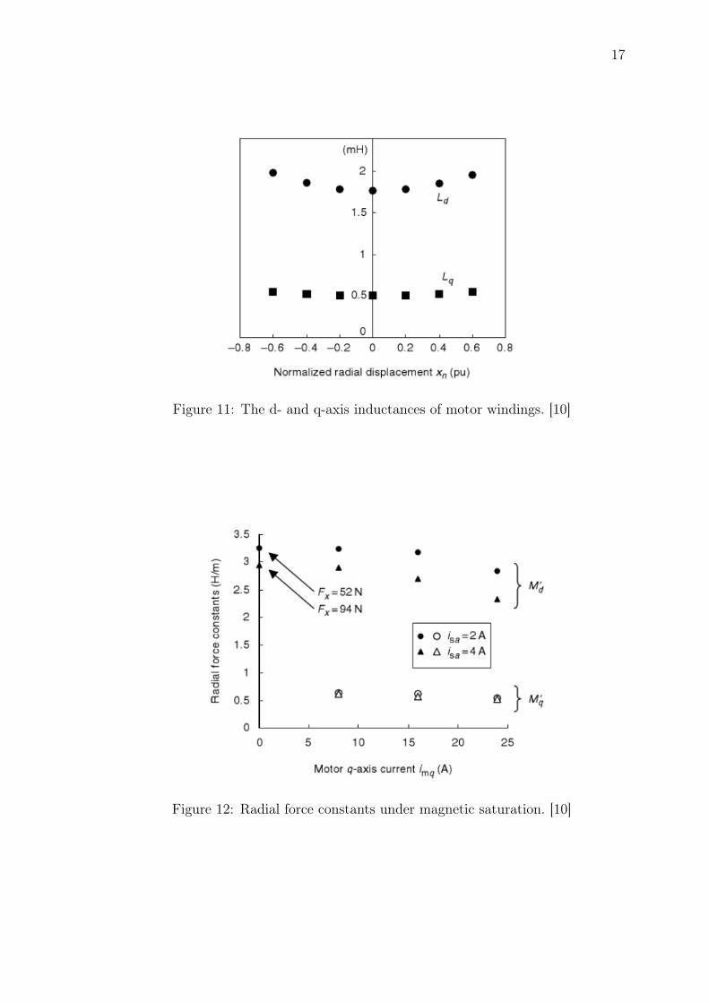
In this final project, inductances Ld and Lq are considered to be constant, while inreal case, the machine saturates and the inductances are not constant and vary asa function of motor currents (or fluxes) and the operation point [13,15]. The valuesof the parameters Ld and Lq have been obtained using Figure 11. Figure 11 showsthe measured d- and q-axis inductances for the motor windings with respect to thenormalized rotor radial displacement. The values of Ld and Lq corresponding tono rotor radial displacement (xn = 0) are used for simulating the operation of themotor. The relationship Ld/Lq = 3 mentioned in [10] for the type of rotor shown inFigure 3 has been also taken into account.
The decision of d - and q-axis suspension force constants values, M ′d and M ′
q, hasbeen carried out using Figure 12. It is important to say that radial force constantsexhibit significant variations in accordance with the torque component current dueto magnetic saturation. Nevertheless, they are considered constants in this study.Figure 12 shows different values of the radial force constants under magnetic satu-ration. In order to obtain the values of M ′
d and M ′q needed for testing the model,
an average of the values that are given in the graph is taken. The values of M ′d and
M ′q obtained in [6] have been also considered and the magnitudes reflected, match
up with the ones obtained in [10].
About ψpm and ψ′pm, in BSyRMs these parameters are zero. The chosen value ofimd,ref , is one of the values used on the tests carried out in [10]. Table 1 includes thenumerical values of the parameters that are used in the machine dynamic model.
Table 1: BSyRM parameters.Parameter Symbol ValueDirect-axis inductance Ld 1.75 mHQuadrature-axis inductance Lq 0.5 mHDirect-axis suspension force constant M ′
d 3.1 H/mQuadrature-axis suspension force constant M ′
q 0.6 H/mPermanent magnets flux linkage ψpm 0 WbSuspension force constant ψ′pm 0 Wb/mMoment of inertia Jtot 0.0001 kgm2
Direct-axis motor reference current imd,ref 8 A
17
Figure 11: The d- and q-axis inductances of motor windings. [10]
Figure 12: Radial force constants under magnetic saturation. [10]
18
3 Vector control
3.1 Vector control theory in bearingless motors
Vector control theory provides a control strategy to regulate the rotational torqueas well as the radial force.
Bearingless synchronous reluctance motors need two different control systems, onefor the motor and one for the suspension. The motor control is responsible forgenerating the revolving magnetic field for torque production and it regulates theinstantaneous rotational torque. The suspension control generates additional mag-netic fields and it regulates the radial force. Due to the radial force generated inBSyRMs, both control systems are linked and have dependent relationships.
The control that have been developed for this final project is a basic control. Thecontrollers implemented are enough for the goal of this final project. This controlwill be improved in future studies.
3.1.1 Motor control system
The motor control is based on the relationships between torque and current. Torqueand current are closely related. In AC motors, in order to control the torque, boththe amplitude and phase angle of the currents have to be regulated.
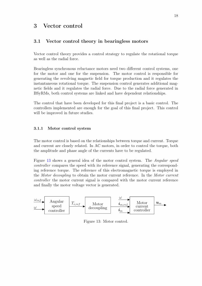
Figure 13 shows a general idea of the motor control system. The Angular speedcontroller compares the speed with its reference signal, generating the correspond-ing reference torque. The reference of this electromagnetic torque is employed inthe Motor decoupling to obtain the motor current reference. In the Motor currentcontroller the motor current signal is compared with the motor current referenceand finally the motor voltage vector is generated.
Angularspeed
controller
Motordecoupling
Motorcurrentcontroller
ωref
ωTe,ref im,ref um
im
ω
Figure 13: Motor control.
19
3.1.2 Suspension control system
The suspension control system is necessary for controlling the radial force generatedby the suspension windings and keep the center of the shaft in the optimal position.
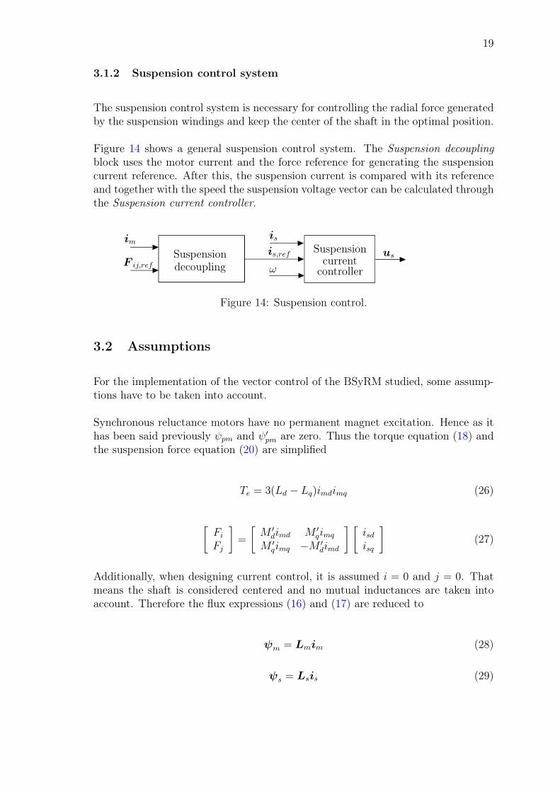
Figure 14 shows a general suspension control system. The Suspension decouplingblock uses the motor current and the force reference for generating the suspensioncurrent reference. After this, the suspension current is compared with its referenceand together with the speed the suspension voltage vector can be calculated throughthe Suspension current controller.
Suspensiondecoupling
Suspensioncurrentcontroller
usF ij,ref
is,ref
isim
ω
Figure 14: Suspension control.
3.2 Assumptions
For the implementation of the vector control of the BSyRM studied, some assump-tions have to be taken into account.
Synchronous reluctance motors have no permanent magnet excitation. Hence as ithas been said previously ψpm and ψ′pm are zero. Thus the torque equation (18) andthe suspension force equation (20) are simplified
Te = 3(Ld − Lq)imdimq (26)
[FiFj
]=
[M ′
dimd M ′qimq
M ′qimq −M ′
dimd
] [isdisq
](27)
Additionally, when designing current control, it is assumed i = 0 and j = 0. Thatmeans the shaft is considered centered and no mutual inductances are taken intoaccount. Therefore the flux expressions (16) and (17) are reduced to
ψm = Lmim (28)
ψs = Lsis (29)
20
If (28) and (29) are substituted in the motor and suspension voltage equations, (13)and (14), the following expressions are obtained:
Lmdimdt
= um − (Rm + J2ωLm)im (30)
Lsdisdt
= us − (Rs + JωLs)is (31)
The current control implementation of the motor and suspension will be based onthese expressions.
3.3 Current controller
The general procedure that has to be followed for the implementation of the one-degree-of-freedom controller needed for the current controller is described below.This procedure is based on [16,17].
First of all is necessary to obtain the transfer function Ge of the electrical dynamicsfrom u′ to i. This procedure has to be done for the motor and suspension equations.Thus general expressions are used and later, the equations for each case are specified.
Start from a general equation similar to (30) and (31)
Ldi
dt= u−Ri− JωLi (32)
where i and u are the general current and voltage space vectors, R is the generalresistance and L is the general inductance matrix.
A new voltage variable
u′ = u− JωLi (33)
is defined to compensate the voltage JωLi. Hence the system
Ldi
dt= u′ −Ri (34)
becomes linear and it is less complicated to design the current controller.
21
Applying the Laplace transform
sLi(s) = u′(s)−Ri(s) (35)
Finally the transfer function Ge from the new voltage variable, u′, to the current,i, is obtained
Ge(s) =1
sL+R(36)
It is important to mention that the equation (36) has been written in scalar formto aid the understanding of the expressions. Nevertheless, the specific equations forthe motor and suspension have a matrix form because of the inductance matrices.
The specific motor and suspension expressions for equation (32) are
Lmdimdt
= um −Rmim − J2ωLmim (37)
Lsdisdt
= us −Rsis − JωLsis (38)
Therefore, the specific motor and suspension transfer functions from equation (36)in matrix form, as is was said previously, are
Ge,m(s) = (sLm +RmI)−1 (39)
Ge,s(s) = (sLs +RsI)−1 (40)
Once the transfer function has been calculated, the controller can be obtained.As previously, scalar variables are used in the explanation and matrix expressionsare used in the specific final equations of the motor and suspension. A simpleproportional-integral (PI) controller is sufficient for the propose of this final project
Fc(s) = Kp +Ki
s(41)
22
where Kp and Ki are the general proportional and integral gains. Since good esti-mates of the motor parameters are known, they can be used to select the controllerparameters Kp and Ki. The following procedure is employed to obtain these param-eters.
The closed-loop transfer function from iref to i should be
Gcc(s) =αc
s+ αc=
1
sτc + 1(42)
αc =1
τc(43)
where αc is the general current control bandwidth and τc is the general closed-loopelectrical time constant.
Known that Gcc(s) can be also expressed as
Gcc(s) =Fc(s)Ge(s)
1 + Fc(s)Ge(s)(44)
Fc(s)Ge(s) =αcs
(45)
the desired closed-loop system is obtained
Fc(s) =αcsG−1e (s) =
αcs(sL+R) = αcL+
αcR
s(46)
That is,
Kp = αcL (47)
Ki = αcR (48)
If the equation (41) is specified for the motor and suspension cases, the PI-controllers
23
become
F c,m(s) =Kpm +1
sKim (49)
F c,s(s) =Kps +1
sKis (50)
whereKpm andKim are the proportional and integral motor gain matrices andKps
and Kis are the proportional and integral suspension gain matrices.
From equations (47) and (48), the specific expressions for motor and suspensioncontroller parameters are
Kpm = αcmLm (51)
Kim = αcmRmI (52)
Kps = αcsLs (53)
Kis = αcsRsI (54)
where αcm and αcs are the motor and suspension current control closed-loop systembandwidth, respectively.
It is important to mention that Lm and Ls are matrices, but Rm and Rs are scalars.Hence when implementing the equations it is needed to multiply Rm and Rs by theidentity matrix I.
Figure 20 and Figure 21, included in Section 4.2, show the implementation inSimulink of these motor and current controllers, respectively.
3.4 Decoupling controller
The motor torque flux causes cross couplings in suspension force generation. Hencethe BSyRM requires a decoupling controller between the motor torque current andthe suspension force in order to realize the stable operation under torque-load con-ditions [6, 11]. A BSyRM includes motor and suspension windings. Thus two de-coupling controllers are needed, one for the motor and one for the suspension.
24
The motor decoupling implementation is based on equation (26), used in the form
imq =Te
3(Ld − Lq)imd(55)
so imq,ref can be calculated and together with imd,ref , the reference vector im,ref canbe obtained.
The suspension decoupling includes the implementation of the equation (27) in thefollowing form:
[isdisq
]=
[M ′
dimd M ′qimq
M ′qimq −M ′
dimd
]−1 [FiFj
](56)
so once calculated isd and isq, the vector is,ref is obtained.
Figure A7 and Figure A8, included in Appendix A, show the implementation inSimulink of both decoupling controllers.
3.5 Parameters
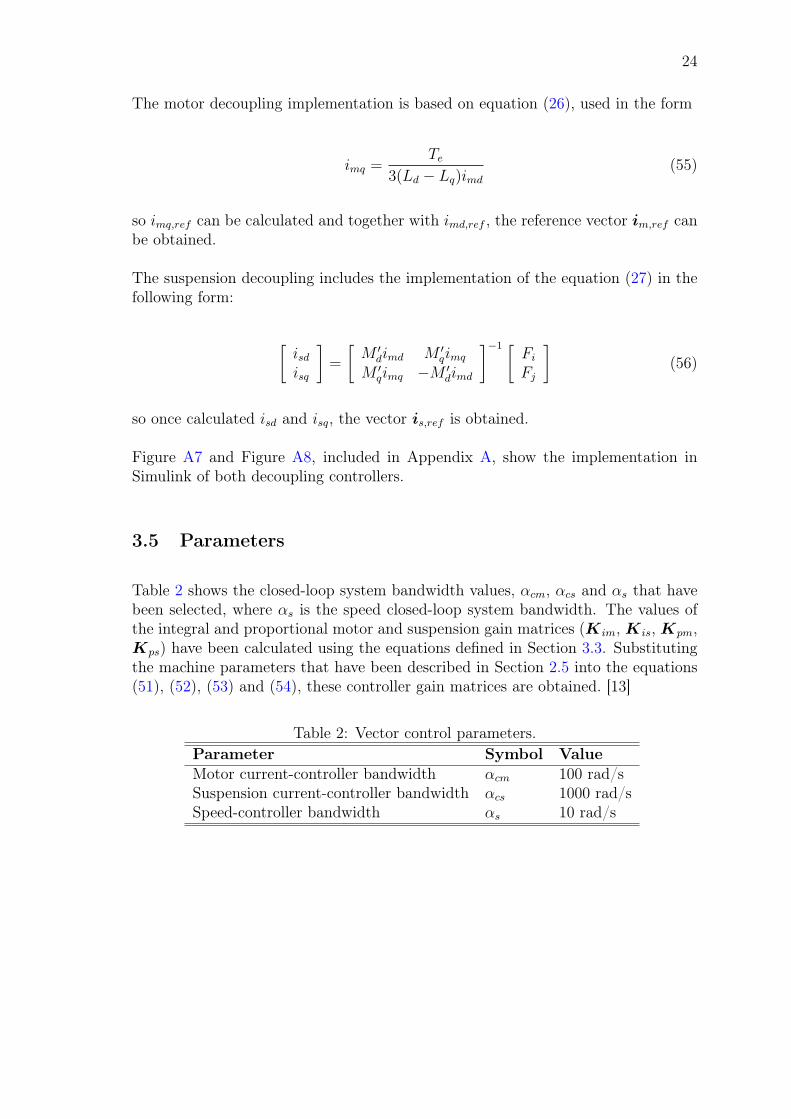
Table 2 shows the closed-loop system bandwidth values, αcm, αcs and αs that havebeen selected, where αs is the speed closed-loop system bandwidth. The values ofthe integral and proportional motor and suspension gain matrices (Kim, Kis, Kpm,Kps) have been calculated using the equations defined in Section 3.3. Substitutingthe machine parameters that have been described in Section 2.5 into the equations(51), (52), (53) and (54), these controller gain matrices are obtained. [13]
Table 2: Vector control parameters.Parameter Symbol ValueMotor current-controller bandwidth αcm 100 rad/sSuspension current-controller bandwidth αcs 1000 rad/sSpeed-controller bandwidth αs 10 rad/s
25
4 Simulink model
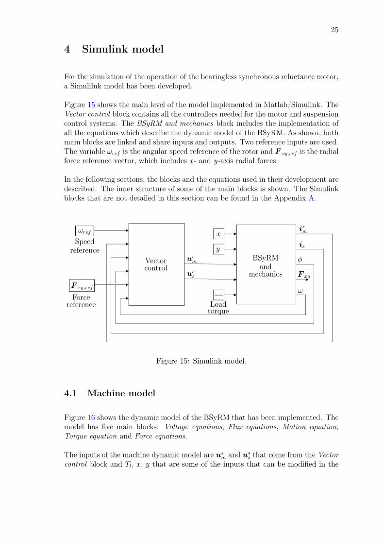
For the simulation of the operation of the bearingless synchronous reluctance motor,a Simulilnk model has been developed.
Figure 15 shows the main level of the model implemented in Matlab/Simulink. TheVector control block contains all the controllers needed for the motor and suspensioncontrol systems. The BSyRM and mechanics block includes the implementation ofall the equations which describe the dynamic model of the BSyRM. As shown, bothmain blocks are linked and share inputs and outputs. Two reference inputs are used.The variable ωref is the angular speed reference of the rotor and F xy,ref is the radialforce reference vector, which includes x - and y-axis radial forces.
In the following sections, the blocks and the equations used in their development aredescribed. The inner structure of some of the main blocks is shown. The Simulinkblocks that are not detailed in this section can be found in the Appendix A.
Speedreference
Forcereference
x
y
Loadtorque
Vectorcontrol
BSyRMand
mechanics
ism
is
F xy
φ
ω
usm
uss
ωref
F xy,ref
Figure 15: Simulink model.
4.1 Machine model
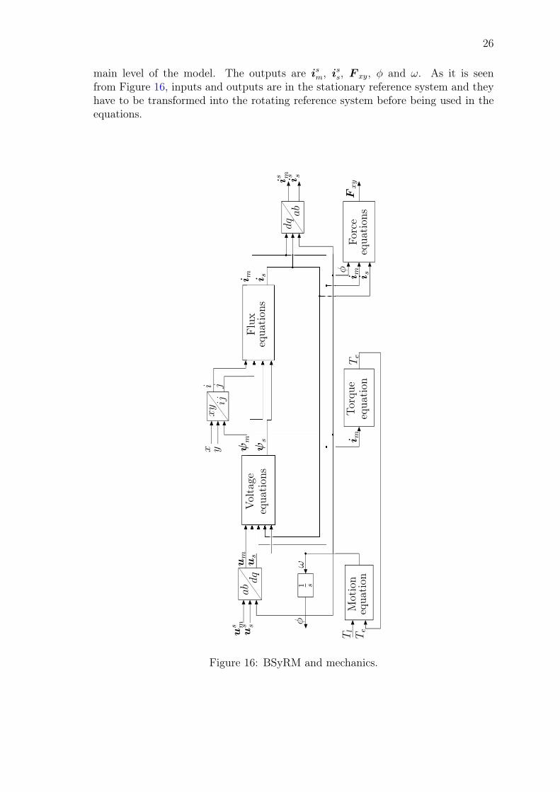
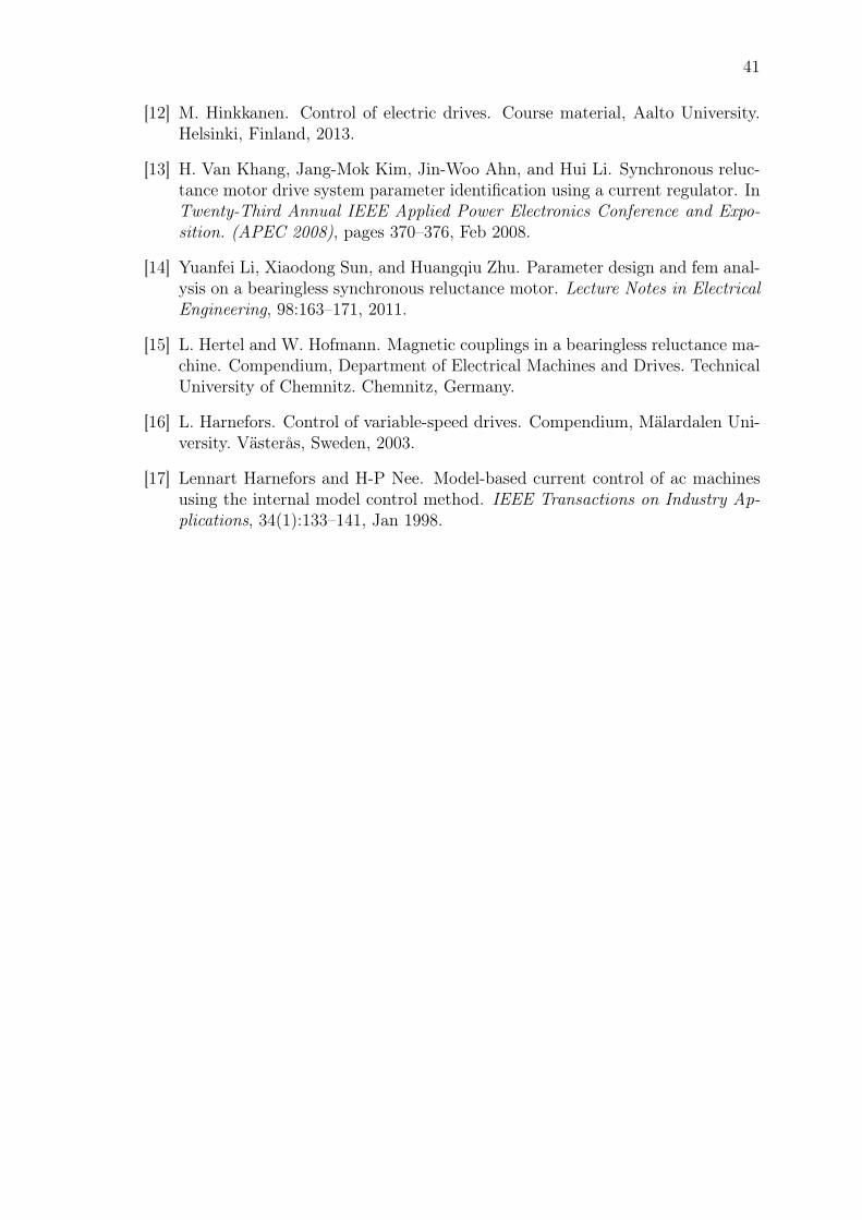
Figure 16 shows the dynamic model of the BSyRM that has been implemented. Themodel has five main blocks: Voltage equations, Flux equations, Motion equation,Torque equation and Force equations.
The inputs of the machine dynamic model are usm and uss that come from the Vectorcontrol block and Tl, x, y that are some of the inputs that can be modified in the
26
main level of the model. The outputs are ism, iss, F xy, φ and ω. As it is seen
from Figure 16, inputs and outputs are in the stationary reference system and theyhave to be transformed into the rotating reference system before being used in theequations.
Force
equa
tion
sTo
rque
equa
tion
Motion
equa
tion
Voltage
equa
tion
sFlux
equa
tion
s
dqab
xy ij
us mus s φ
i m
Tl
Te
ω
x yi j
ψm
ψs
i s
i m
umus
φi m i s
Fxyis m is s
Te
abdq
1 s
Figure 16: BSyRM and mechanics.
27
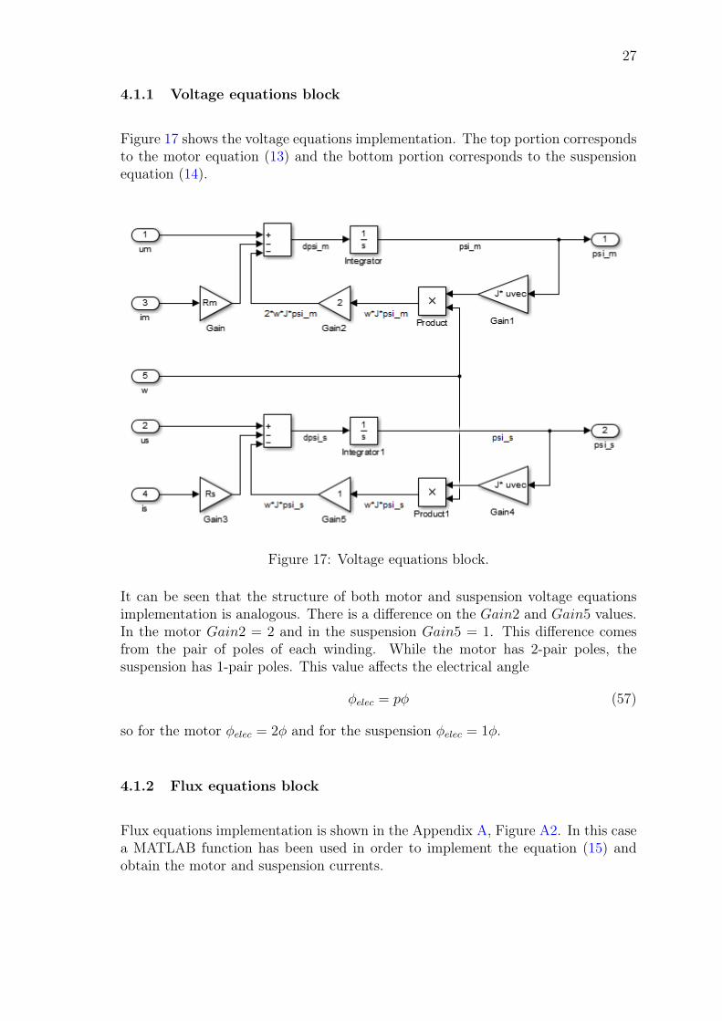
4.1.1 Voltage equations block
Figure 17 shows the voltage equations implementation. The top portion correspondsto the motor equation (13) and the bottom portion corresponds to the suspensionequation (14).
Figure 17: Voltage equations block.
It can be seen that the structure of both motor and suspension voltage equationsimplementation is analogous. There is a difference on the Gain2 and Gain5 values.In the motor Gain2 = 2 and in the suspension Gain5 = 1. This difference comesfrom the pair of poles of each winding. While the motor has 2-pair poles, thesuspension has 1-pair poles. This value affects the electrical angle
φelec = pφ (57)
so for the motor φelec = 2φ and for the suspension φelec = 1φ.
4.1.2 Flux equations block
Flux equations implementation is shown in the Appendix A, Figure A2. In this casea MATLAB function has been used in order to implement the equation (15) andobtain the motor and suspension currents.
28
4.1.3 Torque and motion equations blocks
Torque equation block is shown in the Appendix A, Figure A3. For implementingthe torque equation (18), a MATLAB function has been chosen.
Motion equation (19) is quite simple to implement and it is shown in the AppendixA, Figure A4. It has been build using common blocks from the Simulink library.
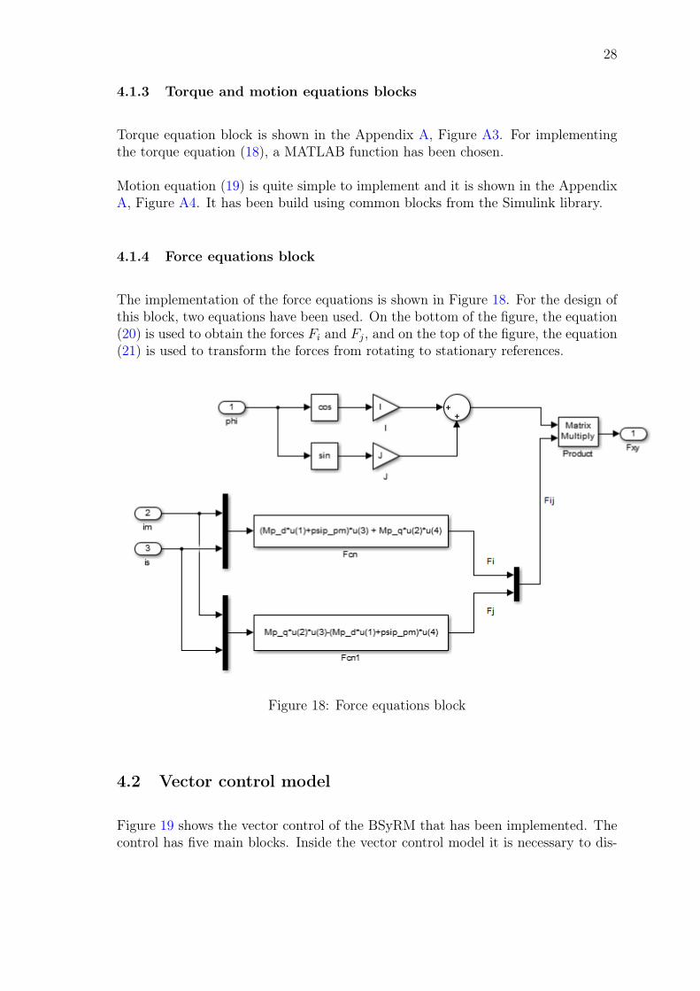
4.1.4 Force equations block
The implementation of the force equations is shown in Figure 18. For the design ofthis block, two equations have been used. On the bottom of the figure, the equation(20) is used to obtain the forces Fi and Fj, and on the top of the figure, the equation(21) is used to transform the forces from rotating to stationary references.
Figure 18: Force equations block
4.2 Vector control model
Figure 19 shows the vector control of the BSyRM that has been implemented. Thecontrol has five main blocks. Inside the vector control model it is necessary to dis-
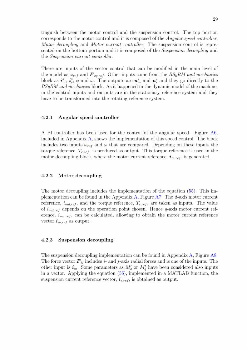
29
tinguish between the motor control and the suspension control. The top portioncorresponds to the motor control and it is composed of the Angular speed controller,Motor decoupling and Motor current controller. The suspension control is repre-sented on the bottom portion and it is composed of the Suspension decoupling andthe Suspension current controller.
There are inputs of the vector control that can be modified in the main level ofthe model as ωref and F xy,ref . Other inputs come from the BSyRM and mechanicsblock as ism, i
ss, φ and ω. The outputs are usm and uss and they go directly to the
BSyRM and mechanics block. As it happened in the dynamic model of the machine,in the control inputs and outputs are in the stationary reference system and theyhave to be transformed into the rotating reference system.
4.2.1 Angular speed controller
A PI controller has been used for the control of the angular speed. Figure A6,included in Appendix A, shows the implementation of this speed control. The blockincludes two inputs ωref and ω that are compared. Depending on these inputs thetorque reference, Te,ref , is produced as output. This torque reference is used in themotor decoupling block, where the motor current reference, im,ref , is generated.
4.2.2 Motor decoupling
The motor decoupling includes the implementation of the equation (55). This im-plementation can be found in the Appendix A, Figure A7. The d -axis motor currentreference, imd,ref , and the torque reference, Te,ref , are taken as inputs. The valueof imd,ref depends on the operation point chosen. Hence q-axis motor current ref-erence, imq,ref , can be calculated, allowing to obtain the motor current referencevector im,ref as output.
4.2.3 Suspension decoupling
The suspension decoupling implementation can be found in Appendix A, Figure A8.The force vector F ij includes i - and j -axis radial forces and is one of the inputs. Theother input is im. Some parameters as M ′
d or M ′q have been considered also inputs
in a vector. Applying the equation (56), implemented in a MATLAB function, thesuspension current reference vector, is,ref , is obtained as output.
30
Ang
ular
speed
controller
Motor
decoup
ling
Suspension
decoup
ling
Motor
current
controller
Suspension
current
controller
ab
dq
dq
ab
ab
ab
dq
dq
xy
ij
ωref ω
Te,ref
i m,ref
i m
φ
is m
us m
um
Fxy,ref
us s
us
Fij,ref
i s,ref
is si s
i s1
i s,ref
1us1
ref 1
ref
ref 1
ref
Figure 19: Vector control.
31
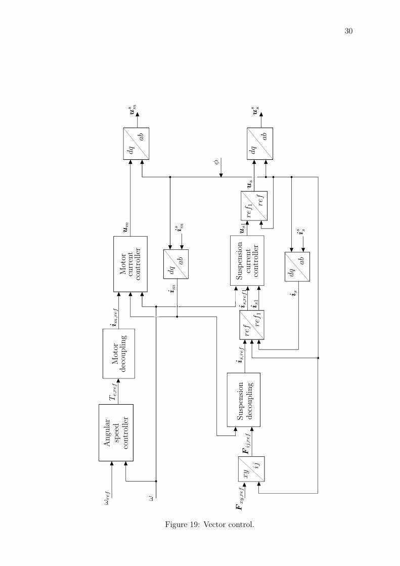
4.2.4 Motor current controller
The procedure described in Section 3.3 has been followed for the implementation ofthe motor current controller. Equations (37), (39), (49), (51) and (52) have beenconsidered. Figure 20 shows the interior of the block developed. The variables im,ref ,im and ω are the inputs and the output obtained is um. This voltage is transformedlater from rotating to stationary coordinates and it will be one of the outputs of theVector control block that becomes an input for the BSyRM and mechanics block.
Figure 20: Motor current controller.
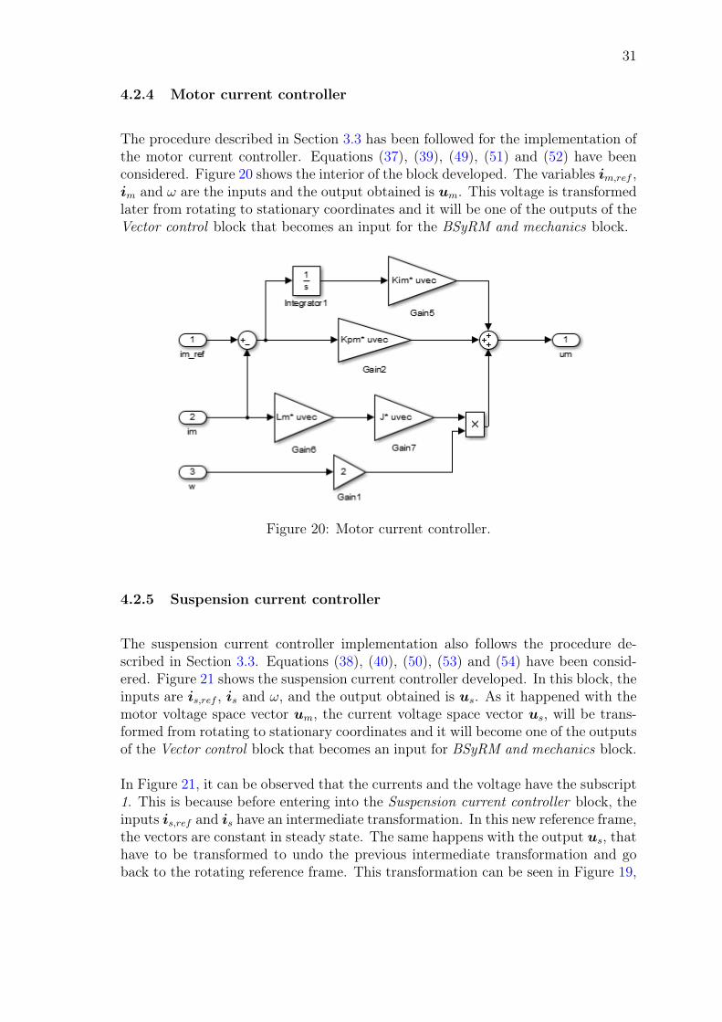
4.2.5 Suspension current controller
The suspension current controller implementation also follows the procedure de-scribed in Section 3.3. Equations (38), (40), (50), (53) and (54) have been consid-ered. Figure 21 shows the suspension current controller developed. In this block, theinputs are is,ref , is and ω, and the output obtained is us. As it happened with themotor voltage space vector um, the current voltage space vector us, will be trans-formed from rotating to stationary coordinates and it will become one of the outputsof the Vector control block that becomes an input for BSyRM and mechanics block.
In Figure 21, it can be observed that the currents and the voltage have the subscript1. This is because before entering into the Suspension current controller block, theinputs is,ref and is have an intermediate transformation. In this new reference frame,the vectors are constant in steady state. The same happens with the output us, thathave to be transformed to undo the previous intermediate transformation and goback to the rotating reference frame. This transformation can be seen in Figure 19,
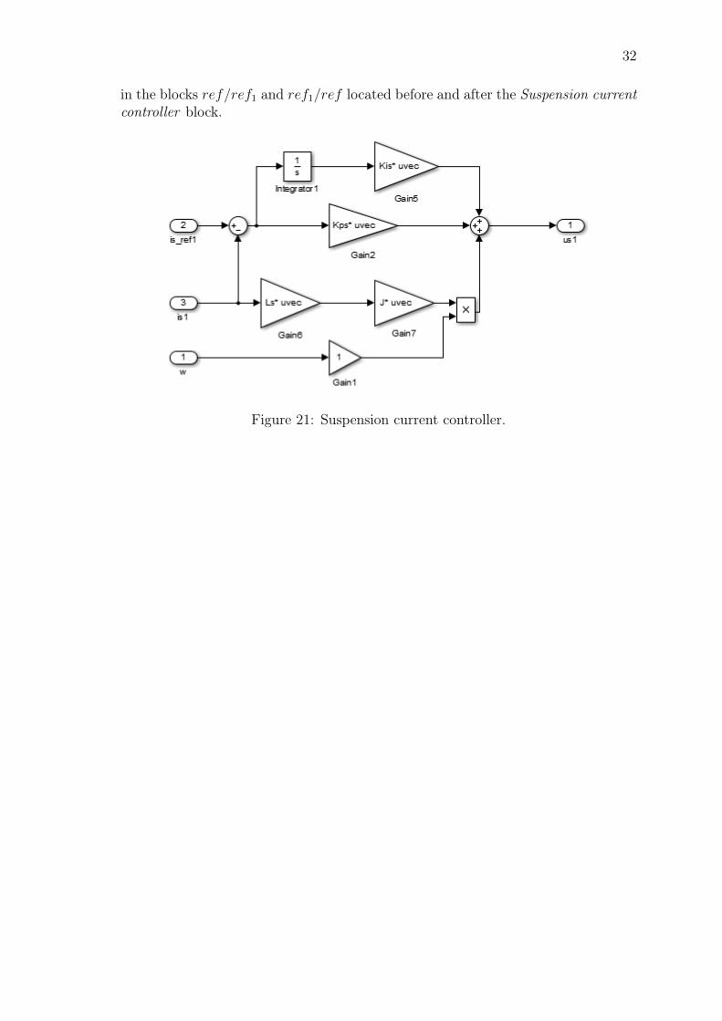
32
in the blocks ref/ref1 and ref1/ref located before and after the Suspension currentcontroller block.
Figure 21: Suspension current controller.
33
5 Simulation results
Different cases have been tested with the Simulink model developed. In each case,various waveforms are shown to verify the correct operation of the machine and itscontrol.
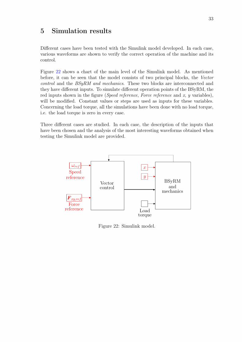
Figure 22 shows a chart of the main level of the Simulink model. As mentionedbefore, it can be seen that the model consists of two principal blocks, the Vectorcontrol and the BSyRM and mechanics. These two blocks are interconnected andthey have different inputs. To simulate different operation points of the BSyRM, thered inputs shown in the figure (Speed reference, Force reference and x, y variables),will be modified. Constant values or steps are used as inputs for these variables.Concerning the load torque, all the simulations have been done with no load torque,i.e. the load torque is zero in every case.
Three different cases are studied. In each case, the description of the inputs thathave been chosen and the analysis of the most interesting waveforms obtained whentesting the Simulink model are provided.
Speedreference
Forcereference
x
y
Loadtorque
Vectorcontrol
BSyRMand
mechanicsF xy,ref
ωref
Figure 22: Simulink model.
34
5.1 Case 1
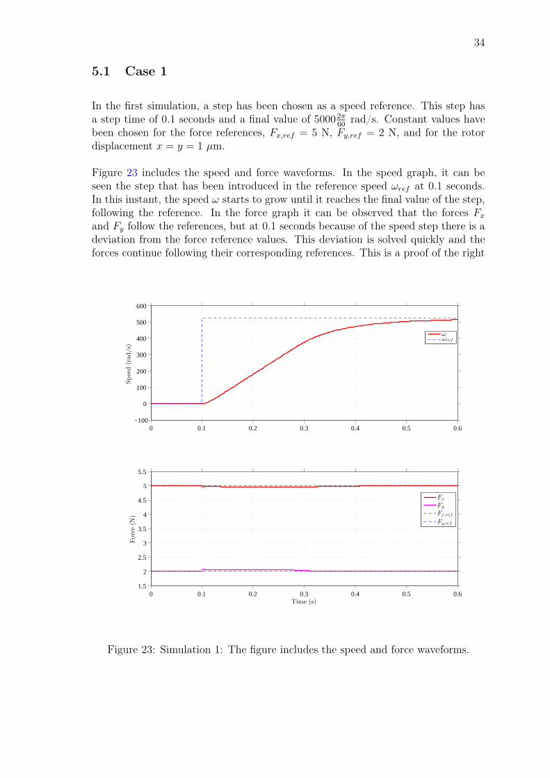
In the first simulation, a step has been chosen as a speed reference. This step hasa step time of 0.1 seconds and a final value of 50002π
60rad/s. Constant values have
been chosen for the force references, Fx,ref = 5 N, Fy,ref = 2 N, and for the rotordisplacement x = y = 1 µm.
Figure 23 includes the speed and force waveforms. In the speed graph, it can beseen the step that has been introduced in the reference speed ωref at 0.1 seconds.In this instant, the speed ω starts to grow until it reaches the final value of the step,following the reference. In the force graph it can be observed that the forces Fxand Fy follow the references, but at 0.1 seconds because of the speed step there is adeviation from the force reference values. This deviation is solved quickly and theforces continue following their corresponding references. This is a proof of the right
0 0.1 0.2 0.3 0.4 0.5 0.6−100
0
100
200
300
400
500
600
Speed(rad/s)
ωωref
0 0.1 0.2 0.3 0.4 0.5 0.61.5
2
2.5
3
3.5
4
4.5
5
5.5
Time (s)
Force(N
)
Fx
Fy
Fx,ref
Fy,ref
Figure 23: Simulation 1: The figure includes the speed and force waveforms.
35
operation of the control developed.
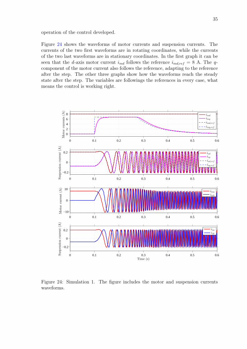
Figure 24 shows the waveforms of motor currents and suspension currents. Thecurrents of the two first waveforms are in rotating coordinates, while the currentsof the two last waveforms are in stationary coordinates. In the first graph it can beseen that the d -axis motor current imd follows the reference imd,ref = 8 A. The q-component of the motor current also follows the reference, adapting to the referenceafter the step. The other three graphs show how the waveforms reach the steadystate after the step. The variables are followings the references in every case, whatmeans the control is working right.
0 0.1 0.2 0.3 0.4 0.5 0.6
0
2
4
6
8
Motorcurrents
(A)
imd
imq
imd,ref
imq,ref
0 0.1 0.2 0.3 0.4 0.5 0.6
−0.2
0
0.2
Suspensioncurrent(A
)
isdisqisd,refisq,ref
0 0.1 0.2 0.3 0.4 0.5 0.6
−10
0
10
Motorcurrent(A
)
ima
imb
0 0.1 0.2 0.3 0.4 0.5 0.6
−0.2
0
0.2
Time (s)
Suspensioncurrent(A
)
isaisb
Figure 24: Simulation 1. The figure includes the motor and suspension currentswaveforms.
36
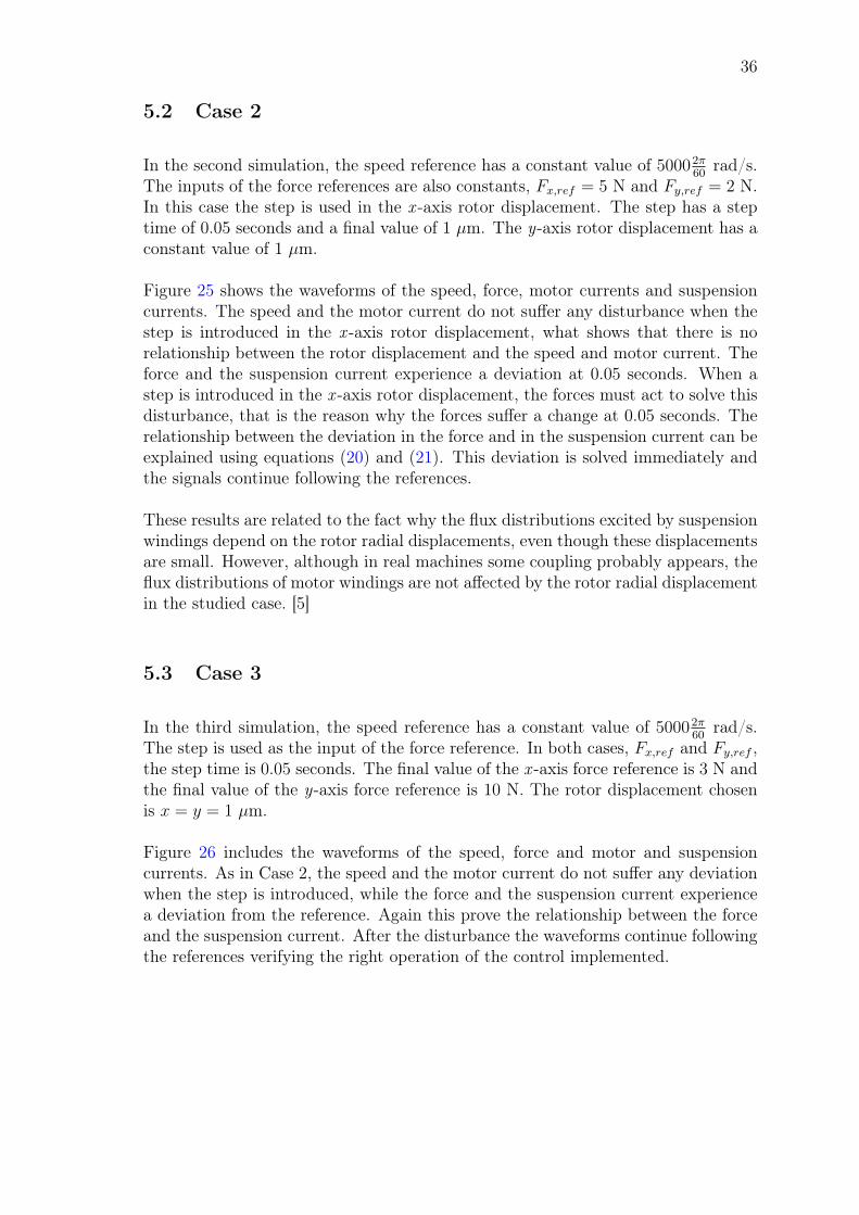
5.2 Case 2
In the second simulation, the speed reference has a constant value of 50002π60
rad/s.The inputs of the force references are also constants, Fx,ref = 5 N and Fy,ref = 2 N.In this case the step is used in the x -axis rotor displacement. The step has a steptime of 0.05 seconds and a final value of 1 µm. The y-axis rotor displacement has aconstant value of 1 µm.
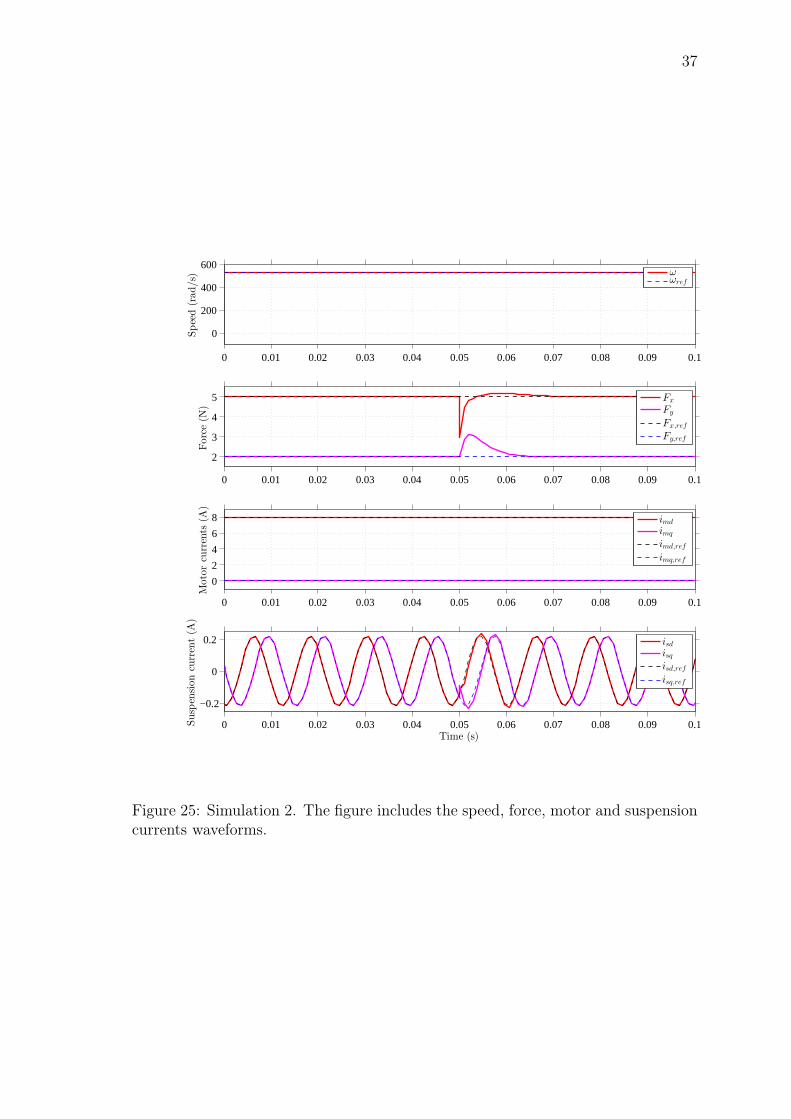
Figure 25 shows the waveforms of the speed, force, motor currents and suspensioncurrents. The speed and the motor current do not suffer any disturbance when thestep is introduced in the x -axis rotor displacement, what shows that there is norelationship between the rotor displacement and the speed and motor current. Theforce and the suspension current experience a deviation at 0.05 seconds. When astep is introduced in the x -axis rotor displacement, the forces must act to solve thisdisturbance, that is the reason why the forces suffer a change at 0.05 seconds. Therelationship between the deviation in the force and in the suspension current can beexplained using equations (20) and (21). This deviation is solved immediately andthe signals continue following the references.
These results are related to the fact why the flux distributions excited by suspensionwindings depend on the rotor radial displacements, even though these displacementsare small. However, although in real machines some coupling probably appears, theflux distributions of motor windings are not affected by the rotor radial displacementin the studied case. [5]
5.3 Case 3
In the third simulation, the speed reference has a constant value of 50002π60
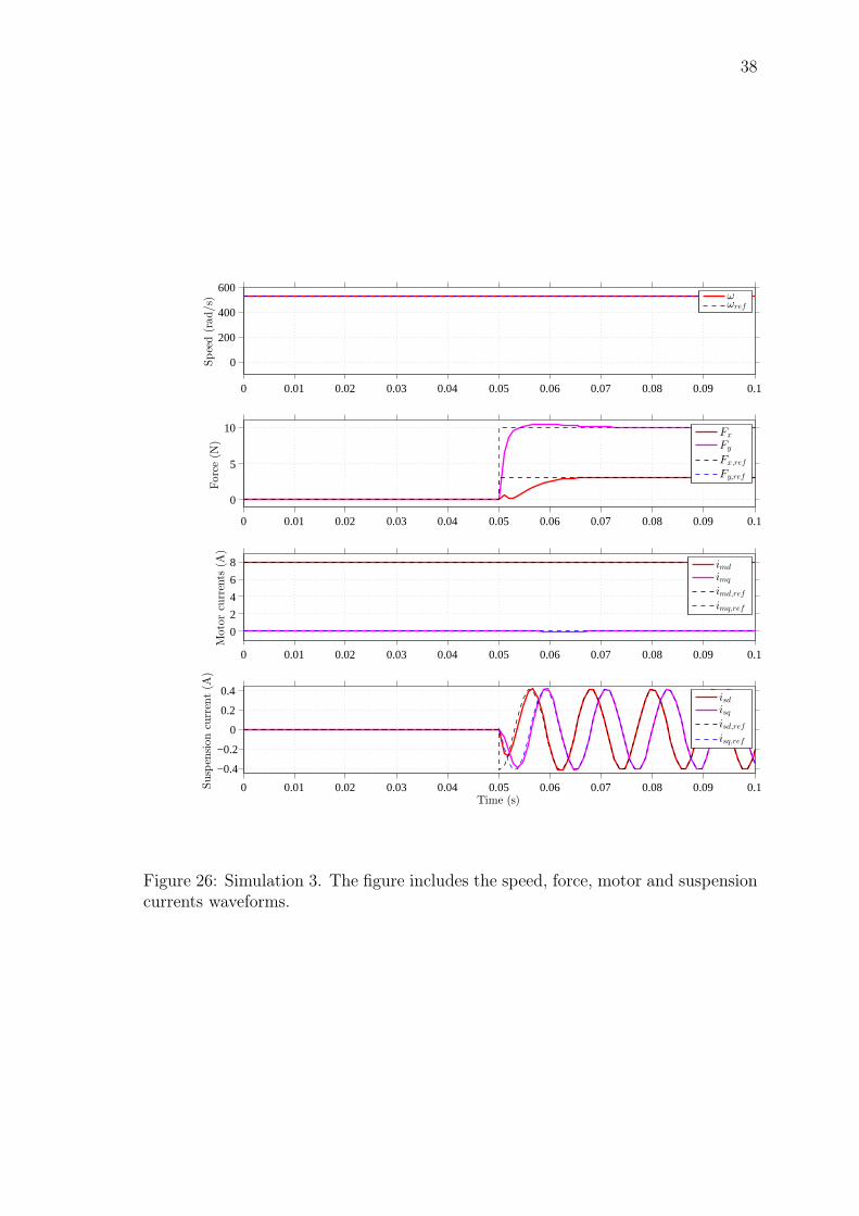
rad/s.The step is used as the input of the force reference. In both cases, Fx,ref and Fy,ref ,the step time is 0.05 seconds. The final value of the x -axis force reference is 3 N andthe final value of the y-axis force reference is 10 N. The rotor displacement chosenis x = y = 1 µm.
Figure 26 includes the waveforms of the speed, force and motor and suspensioncurrents. As in Case 2, the speed and the motor current do not suffer any deviationwhen the step is introduced, while the force and the suspension current experiencea deviation from the reference. Again this prove the relationship between the forceand the suspension current. After the disturbance the waveforms continue followingthe references verifying the right operation of the control implemented.
37
0 0.01 0.02 0.03 0.04 0.05 0.06 0.07 0.08 0.09 0.1
0
200
400
600
Speed(rad/s)
ωωref
0 0.01 0.02 0.03 0.04 0.05 0.06 0.07 0.08 0.09 0.1
2
3
4
5
Force(N
)
Fx
Fy
Fx,ref
Fy,ref
0 0.01 0.02 0.03 0.04 0.05 0.06 0.07 0.08 0.09 0.1
0
2
4
6
8
Motorcurrents
(A)
imd
imq
imd,ref
imq,ref
0 0.01 0.02 0.03 0.04 0.05 0.06 0.07 0.08 0.09 0.1
−0.2
0
0.2
Time (s)
Suspensioncurrent(A
)
isdisqisd,refisq,ref
Figure 25: Simulation 2. The figure includes the speed, force, motor and suspensioncurrents waveforms.
38
0 0.01 0.02 0.03 0.04 0.05 0.06 0.07 0.08 0.09 0.1
0
200
400
600
Speed(rad/s)
ωωref
0 0.01 0.02 0.03 0.04 0.05 0.06 0.07 0.08 0.09 0.1
0
5
10
Force(N
)
Fx
Fy
Fx,ref
Fy,ref
0 0.01 0.02 0.03 0.04 0.05 0.06 0.07 0.08 0.09 0.1
0
2
4
6
8
Motorcurrents
(A)
imd
imq
imd,ref
imq,ref
0 0.01 0.02 0.03 0.04 0.05 0.06 0.07 0.08 0.09 0.1
−0.4
−0.2
0
0.2
0.4
Time (s)
Suspensioncurrent(A
)
isdisqisd,refisq,ref
Figure 26: Simulation 3. The figure includes the speed, force, motor and suspensioncurrents waveforms.
39
6 Conclusions
In this final project, a vector-controlled bearingless synchronous reluctance motordrive has been studied. Both the BSyRM dynamic model and vector control areexplained in detail.
Due to the novelty of BSyRMs some difficulties have emerged during the realisationof this final project. The existence of additional suspension windings for generatingthe radial force has been one of the difficulties, making more difficult to obtain thedynamic model equations. Due to the shortage of these motor types, other problemhas been to find the appropriate machine parameters that permit to simulate theoperation of the motor.
To obtained the dynamic model equations of the BSyRM, more general PMSMequations have been used as a starting point. Later these equations have beenrefined to suit the particular feature of the BSyRM.
In this study of BSyRMs, the magnetic saturation has not been taken into consider-ation to simplify the model. In bearingless motors, one important drawback is thecoupling between motor and bearing system by magnetic saturation. The saturationcan lead to an unstable system performance. Therefore, further studies will includethe modelling of the magnetic saturation.
Improvements to the suspension current controller could be made, but it was con-sidered outside the scope of this final project. However, the suspension currentcontroller should be developed more precisely in later studies. PI-controller param-eters values could also have been further tuned.
To verify the correct operation of the BSyRM model developed, several simula-tions have been tested using the Matlab/Simulink software. The simulation resultspresented, verify that the dynamic model of the BSyRM and the vector controlimplemented, perform well.
40
References
[1] T. Fukao. The evolution of motor drive technologies, development of bearinglessmotors. In The Third International Power Electronics and Motion ControlConference. (IPEMC 2000). Proceedings, volume 1, pages 33–38 vol.1, 2000.
[2] Zengcai Qu, T. Tuovinen, and M. Hinkkanen. Inclusion of magnetic saturationin dynamic models of synchronous reluctance motors. In 2012 XXth Interna-tional Conference on Electrical Machines (ICEM 2012), pages 994–1000, Sept2012.
[3] A. Boglietti, A. Cavagnino, M. Pastorelli, and A. Vagati. Experimental compar-ison of induction and synchronous reluctance motors performance. In FourtiethIAS Annual Meeting. Conference Record of the Industry Applications Confer-ence, volume 1, pages 474–479 Vol. 1, Oct 2005.
[4] A. Chiba, M. Hanazawa, T. Fukao, and M. Azizur Rahman. Effects of magneticsaturation on radial force of bearingless synchronous reluctance motors. IEEETransactions on Industry Applications, 32(2):354–362, Mar 1996.
[5] A. Chiba, T. Deido, T. Fukao, and M.A. Rahman. An analysis of bearinglessac motors. IEEE Transactions on Energy Conversion, 9(1):61–68, Mar 1994.
[6] C. Michioka, T. Sakamoto, O. Ichikawa, A. Chiba, and T. Fukao. A decouplingcontrol method of reluctance-type bearingless motors considering magnetic sat-uration. IEEE Transactions on Industry Applications, 32(5):1204–1210, Sept1996.
[7] A. Chiba, M.A. Rahman, and T. Fukao. Radial force in a bearingless reluctancemotor. IEEE Transactions on Magnetics, 27(2):786–790, Mar 1991.
[8] Hannian Zhang, Huangqiu Zhu, Zhibao Zhang, and Zhiyi Xie. Design andsimulation of control system for bearingless synchronous reluctance motor. InProceedings of the Eighth International Conference on Electrical Machines andSystems. (ICEMS 2005), volume 1, pages 554–558 Vol. 1, Sept 2005.
[9] Xiaodong Sun, Long Chen, and Zebin Yang. Overview of bearinglesspermanent-magnet synchronous motors. IEEE Transactions on Industrial Elec-tronics, 60(12):5528–5538, Dec 2013.
[10] A. Chiba, T. Fukao, O. Ichikawa, M. Oshima, M. Takemoto, and D.G. Dorrell.Magnetic Bearings and Bearingless Drives. Elsevier, Newnes, GBR, 2005. ISBN0 7506 5727 8.
[11] M. Takemoto, K. Yoshida, N. Itasaka, Y. Tanaka, A Chiba, and T. Fukao.Synchronous reluctance type bearingless motors with multi-flux barriers. InPower Conversion Conference - Nagoya. (PCC 2007), pages 1559–1564, April2007.
41
[12] M. Hinkkanen. Control of electric drives. Course material, Aalto University.Helsinki, Finland, 2013.
[13] H. Van Khang, Jang-Mok Kim, Jin-Woo Ahn, and Hui Li. Synchronous reluc-tance motor drive system parameter identification using a current regulator. InTwenty-Third Annual IEEE Applied Power Electronics Conference and Expo-sition. (APEC 2008), pages 370–376, Feb 2008.
[14] Yuanfei Li, Xiaodong Sun, and Huangqiu Zhu. Parameter design and fem anal-ysis on a bearingless synchronous reluctance motor. Lecture Notes in ElectricalEngineering, 98:163–171, 2011.
[15] L. Hertel and W. Hofmann. Magnetic couplings in a bearingless reluctance ma-chine. Compendium, Department of Electrical Machines and Drives. TechnicalUniversity of Chemnitz. Chemnitz, Germany.
[16] L. Harnefors. Control of variable-speed drives. Compendium, Mälardalen Uni-versity. Västerås, Sweden, 2003.
[17] Lennart Harnefors and H-P Nee. Model-based current control of ac machinesusing the internal model control method. IEEE Transactions on Industry Ap-plications, 34(1):133–141, Jan 1998.
42
A Appendix
A.1 Simulink dynamic model
Figure A1: Dynamic model of the machine.
43
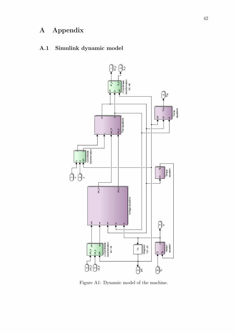
A.1.1 Flux equations
Figure A2: Flux equations block.
The code implemented in the flux MATLAB function is:
f unc t i on [ imd , imq , i sd , i s q ] = fcn (psi_m , psi_s , i , j , params )
%ParamentersLd = params ( 1 ) ;Lq = params ( 2 ) ;Lss = params ( 3 ) ;Md = params ( 4 ) ;Mq = params ( 5 ) ;psi_pm = params ( 6 ) ;psi_pmp = params ( 7 ) ;
%Matr ices and vec to r s d e f i n i t i o n sLm = [Ld , 0 ; 0 , Lq ] ;Ls = [ Lss , 0 ; 0 , Lss ] ;M = [Md∗ i , −Md∗ j ; Mq∗ j , Mq∗ i ] ;psi_pmpv = [ psi_pmp∗ i ; −psi_pmp∗ j ] ;psi_pmv = [ psi_pm ; 0 ] ;
%Currents as a func t i on o f f l u x l i n kag e si s = (Ls − M. ’ /Lm∗M)\( psi_s − psi_pmpv − M. ’ /Lm∗(psi_m − psi_pmv ) ) ;im = Lm\(psi_m − psi_pmv − M∗ i s ) ;i s d = i s ( 1 ) ;i s q = i s ( 2 ) ;imd = im ( 1 ) ;imq = im ( 2 ) ;
44
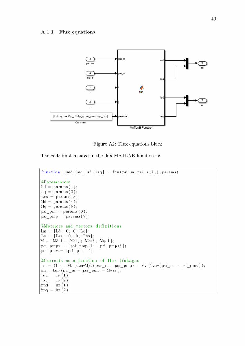
A.1.2 Torque equation
Figure A3: Torque equation block.
The code implemented in the torque MATLAB function is:
f unc t i on Te = fcn ( imd , imq , param)
%ParametersLd = param ( 1 ) ;Lq = param ( 2 ) ;psi_pm = param ( 3 ) ;
%Torque equat ionTe = 3∗ ( (Ld−Lq)∗ imd∗ imq + psi_pm∗ imq ) ;
A.1.3 Motion equation
Figure A4: Motion equation block.
45
A.2 Simulink vector control model
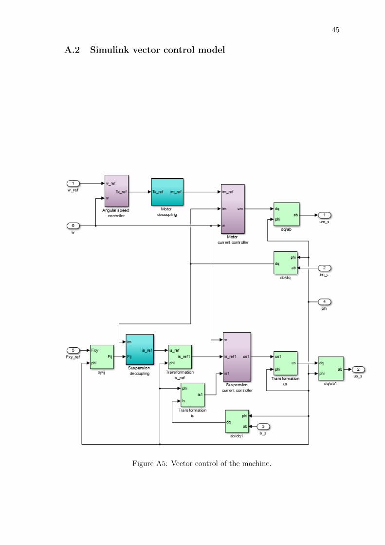
Figure A5: Vector control of the machine.
46
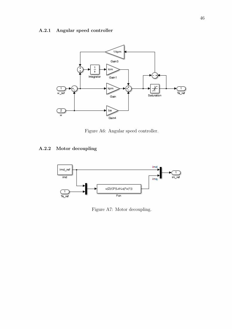
A.2.1 Angular speed controller
Figure A6: Angular speed controller.
A.2.2 Motor decoupling
Figure A7: Motor decoupling.
47
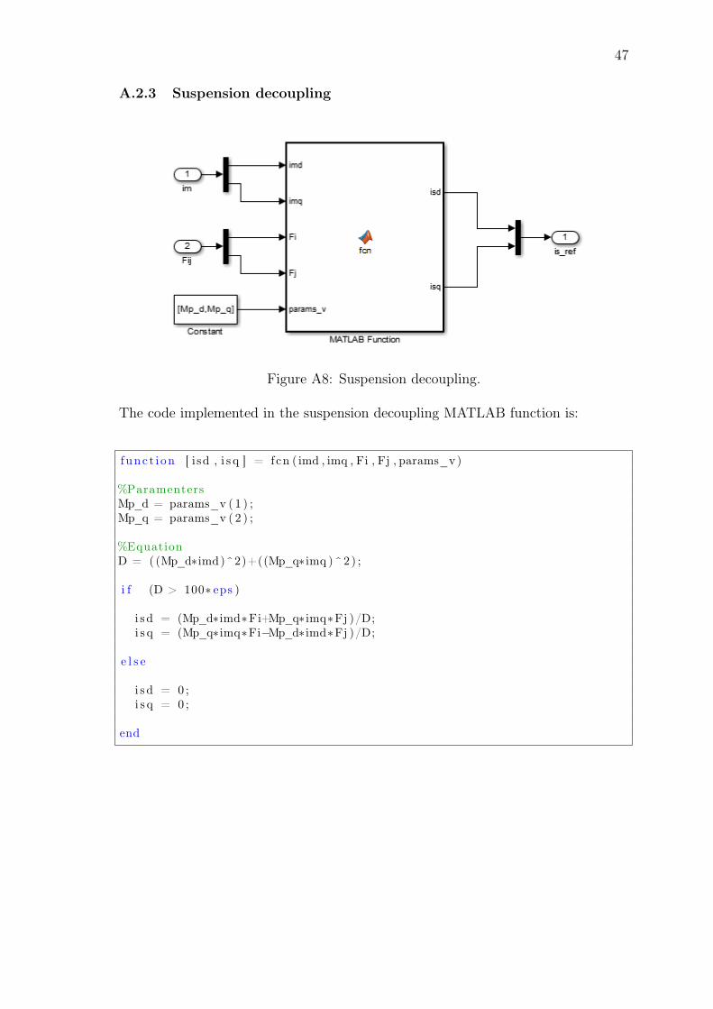
A.2.3 Suspension decoupling
Figure A8: Suspension decoupling.
The code implemented in the suspension decoupling MATLAB function is:
f unc t i on [ i sd , i s q ] = fcn ( imd , imq , Fi , Fj , params_v)
%ParamentersMp_d = params_v ( 1 ) ;Mp_q = params_v ( 2 ) ;
%EquationD = ( (Mp_d∗imd)^2)+((Mp_q∗ imq )^2 ) ;
i f (D > 100∗ eps )
i s d = (Mp_d∗imd∗Fi+Mp_q∗ imq∗Fj )/D;i s q = (Mp_q∗ imq∗Fi−Mp_d∗imd∗Fj )/D;
e l s e
i s d = 0 ;i s q = 0 ;
end