modelling geomorphic systems: fluvial · modelling geomorphic systems: fluvial 2 british society...

British Society for Geomorphology Geomorphological Techniques, Chap. 5, Sec. 6.4 (2015)

Modelling Geomorphic Systems: Fluvial

Michael C. Grenfell1 1 Environmental and Water Science Division, Department of Earth Science, University of the Western Cape, Bellville, 7530, South Africa Email: [email protected]

ABSTRACT: Rivers and floodplains convey and exchange water and all its constituent matter from Earth’s surface to an intra-continental or oceanic sink. The associated processes of flow and flux are the foundation of all ecosystem service provision and human value derived from river environments. Numerical modelling is one of many approaches that may be used to understand these processes. It is an approach that seeks quantitative mechanistic understanding that is critical to enhancing the predictive capacity of river science, and to developing evidence-based management practices. In combination with other approaches, modelling should play a key role in constraining understanding of river responses in an uncertain future. Ongoing improvements in computing power and in the availability and accessibility of fluvial modelling codes have substantially increased the uptake of modelling as a method of investigating fluvial processes and forms. This chapter outlines the physical basis of different types of fluvial model, and illustrates the key considerations needed to select a model code with the necessary numerical complexity, to establish a physical model domain and boundary conditions, to test for sensitivity to domain, boundary and parameter variables, and to evaluate results. KEYWORDS: Numerical modelling, fluvial processes, process-form feedback, morphodynamics

Virtual rivers

Numerical modelling addresses the fundamental mechanisms that drive fluvial processes, and the process-form feedbacks that govern river characteristics, dynamics and socio-ecological value. Numerical models and the virtual rivers they describe are useful tools because they offer the potential for full control over boundary conditions and physical laws (Kleinhans, 2010), thereby providing an abstraction of reality that is modifiable within given physical constraints. This allows one to test hypotheses derived from field data and experiments (Kleinhans, 2010), to evaluate competing explanations, to elucidate key controls (e.g. on chute cutoff; van Dijk et al., 2014), or necessary conditions (e.g. for a meandering river avulsion; Slingerland and Smith, 1998). Such endeavours typically require insight that extends beyond the limits of field observation, or that is difficult to transfer from laboratory experiments.

However, numerical models provide a tool that should be embedded within a broader conceptual approach to understanding rivers, as the greatest potential for full explanation of natural river phenomena arises when results from field measurements, laboratory experiments and numerical modelling converge (Kleinhans, 2010). More broadly, the process itself of building a virtual river can be valuable to force rigour in setting hypotheses and interpreting results for field or experimental studies (Bras et al., 2003). The literature on modelling approaches and applications has burgeoned in recent years, as has the availability of commercial and non-commercial fluvial modelling codes (see Table 1 for examples). The former are subject to licence fees, while the latter comprise research or management-centred software developed by universities, government agencies, or an active free and open source (FOSS) community, and are

ISSN 2047-0371

Modelling Geomorphic Systems: Fluvial 2


Table 1: Examples of fluvial channel and channel-floodplain modelling codes in common use by geomorphologists (crudely ordered according to the dimensionality of process-representation).

Fluvial modelling codes Examples

1D channel and floodplain processes, including sediment transport, erosion and deposition

Example code or numerical basis: HEC-RAS; USACE Hydrologic Engineering Center (available at http://www.hec.usace.army.mil/software/hec-ras/). 2D hydrodynamics currently under development for version 5.

Example model: Energy dissipation in step-pool systems, Chin (2003).

1D morphodynamics for meander migration and floodplain evolution; fixed-width channels

Example code or numerical basis: HIPS Relation (see Parker et al. (2011) for a review).

Example model: bend instability and channel migration in meandering rivers (Ikeda et al., 1981).

1D/quasi 2D bar dynamics at bifurcations

Example code or numerical basis: nodal point relation; Bolla Pittaluga et al. (2003), modified by Kleinhans et al. (2008).

Example model: bifurcation dynamics and avulsion duration in meandering rivers, Kleinhans et al. (2008).

Reduced complexity 2D flow routing, sediment transport and morphodynamics from basin to reach scales; long-term, landscape controls on river form and process (e.g. trunk-tributary interaction)

Example code or numerical basis: CAESAR-Lisflood; Tom Coulthard, Paul Bates (available at http://code.google.com/p/caesar-lisflood/).

Example model: Estimating sediment yield from river basins (Coulthard et al., 2013).

2D depth-averaged morphodynamics for meander migration and floodplain evolution; dynamic width variation

Example code or numerical basis: Nays2D; Asahi et al., 2013 (available at http://i-ric.org/en/).

Example model: co-evolution of river width and sinuosity in a meandering river (Asahi et al., 2013).

2D depth-averaged morphodynamics for multiple-thread channel planform dynamics

Example code or numerical basis: - Delft3D; Deltares (available at

http://oss.deltares.nl/web/delft3d/about). - HSTAR; Andrew Nicholas

Example models: dynamic planform evolution and planform transitions in large alluvial rivers (Nicholas 2013a, 2013b; Schuurman et al., 2013).

2D/quasi-3D hydrodynamics and sediment transport; fixed banklines

Example code or numerical basis: FaSTMECH; USGS Geomorphology and Sediment Transport Laboratory (available at http://i-ric.org/en/).

Example model: bed evolution in flow separation eddies (Nelson and McDonald, 1995).

Full 3D CFD with Large Eddy Simulation and particle tracking

Example code or numerical basis: Hardy et al. (2005).

Example model: Transport of individual particles over a gravel bed (Hardy, 2005).

Note: this list is not exhaustive, and some codes may overlap different application environments (e.g. Delft 3D has been used in quasi-3D mode with fixed banks to investigate the stability of bifurcations, Kleinhans et al., 2008, and in depth-averaged mode with a bank erosion model to investigate dynamic planform evolution, Schuurman et al., 2013). The examples indicate potential codes for use in common applications, with a focus on codes available in the public domain.

http://www.hec.usace.army.mil/software/hec-ras/

http://code.google.com/p/caesar-lisflood/

http://i-ric.org/en/

http://oss.deltares.nl/web/delft3d/about


3 Michael C. Grenfell


typically provided at no cost upon request. To those wishing to learn how to learn about rivers using numerical models, this growth in interest is inspiring, but also daunting. Key challenges lie in finding a code that is fit for purpose, and in understanding important elements of how the code works. The aim of this chapter is to present a simplified general account of key considerations involved in selecting, running and evaluating results of numerical models for fluvial channel and channel-floodplain applications.

Overview

In broad terms, setting up a numerical fluvial model will require: i) decisions on the complexity of process representation, ii) definition of the spatial and temporal domains, iii) definition of boundary conditions and initial conditions, iv) testing for sensitivity to variation in the values of key parameters, and v) confirmation (sensu Oreskes et al., 1994) of results. The process is iterative at all stages; e.g. developing a computational grid requires iterative refinement to meet specified quality criteria, calibration and sensitivity tests may involve iteratively adjusting parameter values to match measurements or define error limits, and confirmation of results is typically expressed in terms of a range of variability in model output derived through iteratively adjusting model variables.

Necessary numerical complexity

All models capable of representing fluvial process-form relations and morphological dynamics achieve three basic things with varying levels of complexity, realism and computational cost (Figure 1): (1) they route water (‘hydrodynamics’); (2) they predict sediment transport based on flow characteristics determined by point (1); and, (3) they update the boundary morphology based on fluxes driven by point (2) (‘morphodynamics’).

Hydrodynamics

Fluvial model codes route water between nodes aligned on a longitudinal profile (1D), or between cells on a grid (2D, quasi-3D or 3D). Some codes combine nodes (for the channel) and a grid (for the floodplain) in lattice-network structures (Bates and De Roo, 2000; Nicholas and Quine, 2007). Each node

or cell has a location that can be defined using a physical spatial coordinate system. Node or cell properties such as elevation, bed characteristics (sediment size, density, porosity, and roughness), and water level are defined using a commensurate physical spatial coordinate system. Water routing schemes calculate fluxes of mass and momentum across the spatial domain and through time according to physical laws that may be represented with varying numerical complexity. One division of this complexity relates to the treatment of momentum, wherein numerical model codes may be grouped as either ‘physics-based’ or ‘reduced-complexity’. Physics-based codes solve the Navier-Stokes equations (for detailed reviews relevant to fluvial geomorphology, see Lane, 1998, Wright and Baker, 2004, and Ingham and Ma, 2005). Several orders of complexity are observed according to the treatment of turbulence in the momentum flux. For geomorphological applications the highest level of complexity is achieved using the ‘Reynolds-averaged Navier Stokes equations’ (RANS). These allow simulation of complex flow structures on relatively high-resolution 3D grids, but the equations must be closed using a turbulence model (Ingham and Ma, 2005). Full 3D RANS codes are required to accurately simulate complex flow structures and to simulate the trajectory of individual particles over an irregular bed (Hardy, 2005, 2008). Within the RANS approach, there are models that represent only the time-averaged flow conditions, and more complex models that are eddy-resolving (e.g. Large Eddy Simulation, LES; Keylock et al., 2005). In LES, a length scale is used to differentiate between large and small eddies, and large eddies are resolved directly on a high-resolution grid, while smaller eddies are parameterised using a sub-grid scale model (Wright and Baker, 2004). LES computations are sensitive to grid resolution and to the method of spatio-temporal discretisation employed (Wright and Baker, 2004). It is important to investigate these issues in code validation documents, especially since turbulence values computed by LES are used in sediment transport equations (discussed in the next section).



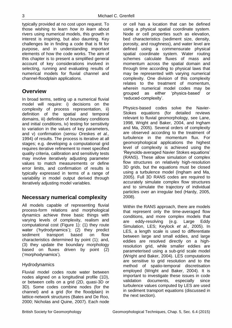
Figure 1: Versatility of numerical modelling in river environments, illustrated through the variety of possible schematisations of the physical space and dynamics of a fluvial geomorphic feature (in this case, a bifurcation) in the computational space of numerical models. a) A photograph of a natural bifurcation (avulsion) on the Mkuze River in eastern South Africa. b) Schematic 1D/quasi-2D nodal point relationship of a bifurcation on a braided river (redrawn from Bolla Pittaluga et al., 2003). c) Curvilinear SWE model grid of an avulsion, with simplified domain geometry (redrawn from Kleinhans et al., 2008). The curvature of the inlet reach may be varied systematically to simulate the effect of the upstream bend configuration on bifurcation dynamics. d) morphodynamic development of bifurcations and an anabranching channel network in a SWE model with a regular grid (after Nicholas, 2013a). Computational demands and process realism increase from b) to d), but the goal of these different approaches varies; c) may be used to test the realism of b), while b) may be used to examine controls on morphodynamics over longer timescales than possible with c). Parameterisation of d) requires an advanced understanding of the controls on bifurcation (such as developed by b) and c)), but seeks to understand the morphodynamics of channel network and coupled channel-floodplain development as a whole.

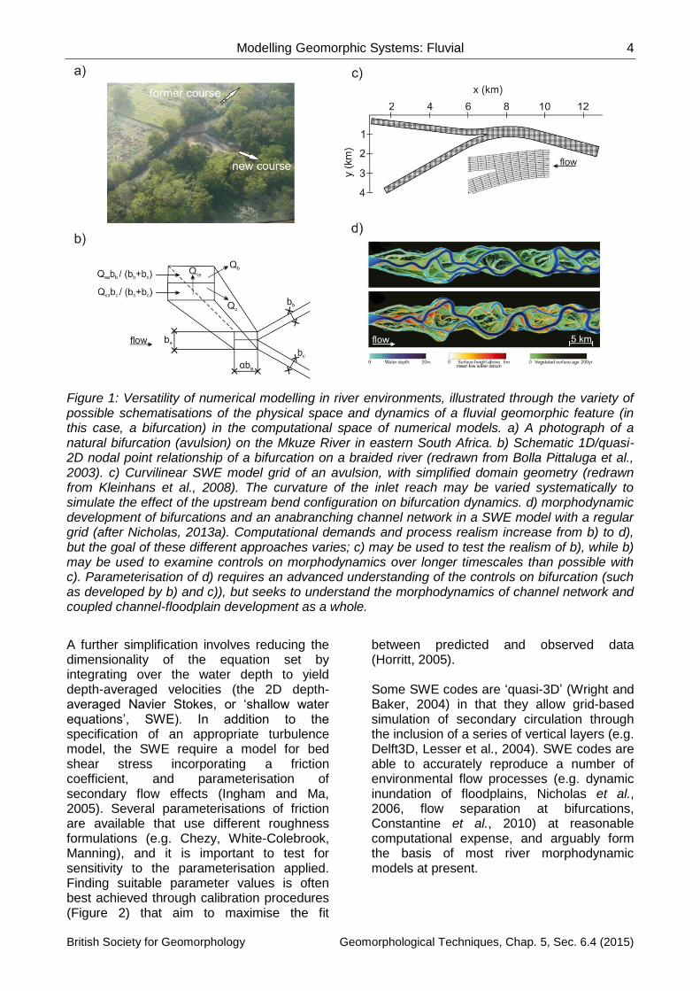
A further simplification involves reducing the dimensionality of the equation set by integrating over the water depth to yield depth-averaged velocities (the 2D depth-averaged Navier Stokes, or ‘shallow water equations’, SWE). In addition to the specification of an appropriate turbulence model, the SWE require a model for bed shear stress incorporating a friction coefficient, and parameterisation of secondary flow effects (Ingham and Ma, 2005). Several parameterisations of friction are available that use different roughness formulations (e.g. Chezy, White-Colebrook, Manning), and it is important to test for sensitivity to the parameterisation applied. Finding suitable parameter values is often best achieved through calibration procedures (Figure 2) that aim to maximise the fit

between predicted and observed data (Horritt, 2005). Some SWE codes are ‘quasi-3D’ (Wright and Baker, 2004) in that they allow grid-based simulation of secondary circulation through the inclusion of a series of vertical layers (e.g. Delft3D, Lesser et al., 2004). SWE codes are able to accurately reproduce a number of environmental flow processes (e.g. dynamic inundation of floodplains, Nicholas et al., 2006, flow separation at bifurcations, Constantine et al., 2010) at reasonable computational expense, and arguably form the basis of most river morphodynamic models at present.



Figure 2: Parameterisation of hydraulic roughness is an inexact science (Horritt, 2005). Calibration seeks parameter values that produce the best fit between model predictions and observations, in this case of floodplain inundation extent (redrawn from Horritt, 2005). Contours represent the fit between inundation extent predicted by a SWE model and that mapped from ERS-1 SAR data.

The dimensionality of the equation set may be further reduced as in the nodal 1D ‘St Venant equations’, implemented in full (e.g. Brunner, 2010) or reduced to the kinematic wave approximation (e.g. Bates and De Roo, 2000). Codes based on the St Venant equations are used extensively to investigate flood inundation over complex topographies (e.g. Nicholas and Walling, 1997). Reduced-complexity codes for channel applications use a simplified treatment of the momentum flux. Initially this involved replacing the momentum equation of the SWE by a steady, uniform flow approximation, with the goal of improving computational efficiency, often at the expense of process realism (see the review by Nicholas and Quine, 2007). Thus, one of the key challenges of reduced-complexity modelling lay in incorporating regional proxies of momentum effects to refine routing rules that otherwise operated exclusively with local (adjacent cells) information. In this regard, examples of important advancements include reducing model sensitivity to grid resolution (discussed later) by calculating slope as a weighted function of local and upstream topographic gradients (Nicholas et

al., 2006), and simulating river meandering by transferring regional information on bend curvature to individual cells (Coulthard and Van De Wiel, 2006). True fluvial geomorphic models go beyond hydrodynamics to include transfer of dissolved or particulate matter (a process-study), or couple sediment fluxes with the morphology and composition of the bounding environment to simulate change (a process-form study; ‘morphodynamics’). These aspects are discussed next.

Sediment transport

Fluvial geomorphic models predict a sediment transport rate at each node or cell, typically as a function of the local transport capacity, using empirical relations based on shear stress or stream power (derived from the hydrodynamics model). It is possible to model the transport of individual particles over an irregular bed using 3D codes (Hardy, 2005), and this may become increasingly important in some gravel bed river applications. However, most present applications in gravel and sand-bed rivers focus on bulk transport of material and the associated morphological response. Several sediment transport formulae are available (e.g. Meyer-Peter and Müller, 1948, Engelund and Hansen, 1967, and van Rijn, 1993). The choice of formula is often a matter of personal preference, and sensitivity to this choice should be assessed. The Meyer-Peter and Müller (1948) formula tends to be favoured for gravel transport (e.g. Paola, 1996, and Nicholas, 2000), while the Engelund and Hansen (1967) formula is commonly applied to model fine gravel and/or sand transport (e.g. Kleinhans et al., 2008, Nicholas, 2013a, and van Dijk et al., 2014). Partheniades (1965) is typically used to model cohesive sediment transport (e.g. Deltares, 2014). Sediment transport over a non-erodible surface (e.g. cohesive floodplain) may be modelled using the approach of Struiksma (1999), which preserves the integrity of local transport capacity relations by applying a correction factor to reduce the transportable layer thickness of the bed (Mosselman, 2005). When considering the direction of sediment transport it is important to note that secondary (helical) flow and gravity-driven



transverse bed slope effects cause deviations between the direction of bed and near-bed sediment transport and that of the flow (Mosselman, 2005). Not all models correct for these effects. Work by Schuurman et al. (2013) and Nicholas (2013a, b) showed that the inclusion of such corrections is necessary to simulate dynamic channel planform evolution: i) secondary circulation corrections are essential to generate high-sinuosity meanders; and, ii) deflection driven by local bed slopes (determined by relative sediment mobility – the ratio of particle fall velocity to shear velocity) controls bar development. In combination with the effects of secondary circulation, these factors control bar morphodynamics, the rate of conversion of bars to floodplain through aggradation (Asahi et al., 2013) and vegetation colonisation, and ultimately channel dimensions. Significant uncertainty remains in the parameterisation of bed slope effects (Mosselman, 2005; Nicholas, 2013a).

Morphodynamics

Fluvial geomorphic models update the morphology of the bounding environment at each node or cell based on the local volume change given by the balance between incoming and outgoing sediment. All forms of sediment mass balance equation are derived from work originally presented by Exner (1920, 1925), which schematises a sediment surface (e.g. hillslope, or channel bed) as a series of layers of known density, thickness, and volume (see Paola and Voller, 2005, for a full review and derivation of different forms of the equations). Such schematisation allows changes in bed level to be determined based on the flux at each control volume (e.g. cell), driven inter alia by the rate of gain or loss of mass within the flow, and horizontal divergence of particle flux within the flow, which are in turn driven by properties of the flow and local morphology (Paola and Voller, 2005).

Spatial domain and sensitivity

Different numerical approaches variously introduce false behaviour in hydraulics (and hence transport and/or morphological change) that is an artefact of the mathematics at play. The key note is that these artefacts may originate from or be expounded by certain aspects of the virtual

environment. One example is numerical diffusion in RANS codes that can be a problem where the grid resolution is low or the grid is poorly aligned with the primary flow direction (Patankar, 1980). For RC codes, grid-dependence of solutions may be unavoidable since the grid structure is an integral part of the process parameterisation (Nicholas, 2005). It is therefore important to understand what the potential sensitivities are for the code being used, and to work to quantify the effects of these sensitivities on model results.

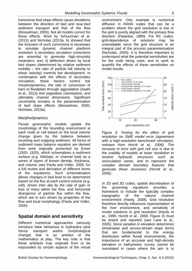
Figure 3: Testing for the effect of grid resolution on SWE model error (agreement with a high-resolution benchmark simulation, redrawn from Horritt et al., 2006). The increase in error with grid cell size is due to the inability of models at lower resolution to resolve hydraulic structures such as recirculation zones, and to represent the complex domain boundary features that generate these structures (Horritt et al., 2006).

In 2D and 3D codes, spatial discretisation of the governing equations provides a framework to include the typically complex topography of the natural channel environment (Hardy, 2008). Grid resolution therefore directly influences representation of the river environment, and sensitivity of model solutions to grid resolution (Hardy et al., 1999; Horritt et al., 2006; Figure 3) must be tested and reported (see Lane et al., 2005). Since variation in elevation determines streamwise and across-stream slope terms that are fundamental to the energy distribution within fluvial environments, the importance of an accurate and high-density elevation or bathymetric survey cannot be overstated in cases where the aim is to



investigate complex 3D flow structures (Horritt et al., 2006; Hardy, 2008), to calibrate turbulence parameters in 2D hydrodynamic models (Williams et al., 2013), or to predict flow paths and sedimentation processes over complex floodplain topography (Nicholas and Mitchell, 2003). Ideally, the point density of a survey would match the grid resolution such that each cell has a measured elevation value. This is achievable in the case of LiDAR, terrestrial laser scanner, multibeam echosounder, or other continuous data. Otherwise, elevation data will comprise a series of points surveyed using ad-hoc, cross-section and/or morphologically-based approaches. These discontinuous data are interpolated onto the grid, thereby introducing an element of uncertainty. Confidence in a morphological survey can be enhanced by understanding the effect of different survey strategies and interpolation methods (see Heritage et al., 2009). Although an accurate initial morphology is typically prized in hydrodynamics applications (especially in 3D models), in the case of morphodynamic models that generate morphology, initial boundary conditions are commonly set using generalised values of key variables (slope, particle size distribution, discharge regime) that are broadly representative of a natural analogue, rather than using a specific set of highly accurate, high resolution field data (e.g. Kleinhans et al., 2008). This is justified because the process representation of a model is unlikely to be consistent with processes operative at a field site (Nicholas, 2005). One approach is to set an initial morphology comprising a plane bed with a constant slope and small white noise elevation perturbations (Nicholas, 2013a). In morphodynamic models it is important that the grid is able to accommodate the dynamics of landforms under investigation such that model output may be evaluated through comparison of properties of elevation change or planform change of modelled and measured environments. In the work of Nicholas (2013a, b) for example, the combination of a simple grid structure that can accommodate both gradual (lateral migration) and abrupt (cutoff, avulsion) channel movements, with a bank erosion

model that preserves bank height, is considered critical to the ability of models to reproduce channels that are similar in form and behaviour to natural analogues.

Temporal domain and sensitivity

Determining an optimum computational time step for a model requires a balance between preservation of numerical stability (improved by decreasing the time step) and computational efficiency (improved by increasing the time step). In codes based on the Navier-Stokes equations, the largest possible time step ensuring preservation of numerical stability may be found using an approach that ensures that hydrodynamic wave propagation does not progress beyond one cell per time step (CFL, Courant-Friedrichs-Lewy condition or number, Courant et al., 1928). The CFL number is determined by model hydrodynamic properties and grid cell dimensions, and most code user manuals discuss its derivation in the context of the numerical procedure applied (e.g. Deltares, 2014). Numerical stability is ensured by scaling the time step according to the CFL condition. Instability is indicated by ‘chequerboard’ oscillations in hydrodynamic properties over a grid or lattice in flow simulations (Bates et al., 2010; Coulthard et al., 2013). In lattice-network codes, numerical instability may be alleviated using a flow limiter (Bates and De Roo, 2000), which results in poor representation of the flow dynamics (Bates et al., 2010), or adaptive time-stepping (Hunter et al., 2005), which greatly increases the computational demand, especially for the high-resolution grids required in some applications. Bates et al. (2010) advanced the approach of Hunter et al. (2005) through incorporating a simple treatment of inertia based on analysis of the St. Venant equations, which allows time steps that scale linearly with the grid cell size according to the CFL condition (reviewed by Coulthard et al., 2013). Some SWE codes use different time steps for hydrodynamic and morphodynamic development by applying a morphological acceleration or scaling factor to allow simulation of long term morphological change (e.g. Lesser et al., 2004; Nicholas, 2013a). Acceleration of morphological change is



achieved by multiplying sediment fluxes at each grid cell and time step by a constant factor, effectively increasing the morphodynamic time step relative to the hydrodynamic one. The selection of a suitable acceleration factor should be based on sensitivity tests (Lesser et al., 2004); for example, Nicholas (2013a) showed that factors in the range 25 to 200 did not yield systematic variation in morphometric attributes of the simulated morphology (e.g. channel geometry, bar dimensions, number of branches).

Inlet/Outlet boundary conditions

Boundary conditions imposed at the inlet and outlet of the computational domain fundamentally influence simulation outcomes, and where a field analogue is considered it is the boundary conditions that define the field data needed to set up simulations (see Lane et al., 1999 and Ingham and Ma, 2005 for full reviews). At the downstream (outlet) boundary a water level is specified that is either fixed through time (for steady flow simulations) or varies in relation to discharge (for unsteady flow simulations). The main upstream (inlet) boundary requirement is a discharge rate and/or velocity profile (for 3D codes) – if the latter is required but could not be determined in the field it is acceptable to use a uniform velocity distribution (e.g. Milan, 2013) provided that the inlet is located far upstream of the region under investigation to allow development of a full flow field (Ingham and Ma, 2005). This is good practice for morphodynamic simulations as well, as morphological change at the inlet is representative of the immediate inlet flow/sediment feed rather than an outcome of channel process-form interaction. Another method of improving the realism of inlet conditions involves the incorporation of an inlet bed perturbation comprising a rocking plane that mimics the slow migration of alternate bars (Nicholas, 2013a). The key point is that boundary perturbations may be needed in morphodynamic models to mimic disturbances that are central to the behaviour of natural systems. Morphodynamic disturbances typically propagate downstream in rivers (although upstream propagation also occurs), and in 1D meander migration models, for example, omitting inlet

perturbations may lead to channel straightening downstream of the inlet over time (Zolezzi and Seminara, 2001).

Confirmation

While hydrodynamic model attributes (e.g. depth, depth-averaged velocity) can be calibrated and confirmed according to their agreement with point or cross-sectional field measurements that are relatively easy to define at discrete points in space and time, morphodynamic model attributes are more difficult to define and thus morphodynamic model confirmation is more challenging (Bras et al., 2003). Confirmation in the latter case typically involves quantifying metrics that describe the morphology and dynamics of the virtual river, and comparing these with measurements from imagery, fieldwork, laboratory experiments or results from other models that make different simplifying assumptions. Metrics used by Schuurman et al. (2013) to evaluate models of large braided sand-bed rivers included bed levels, braiding index, active channel width, bar length and bar shape. The focus of confirmation in morphodynamic modelling is not on reproducing an exact field analogue morphology (a perfect overlay of modelled and field forms), but on mimicking the quantifiable structure and dynamics of the natural environment. The choice of when (in simulation time) to extract data for confirmation purposes tends to vary for hydrodynamic and morphodynamic models. Hydrodynamics simulations are typically run for relatively short timescales over which it is possible to compute an equilibrium solution for steady flow simulations (‘convergence’ for the specified boundary and initial conditions; Lane et al., 2005), and over which unsteady flow dynamics can be compared with field measurements. Morphodynamics problems operate at longer timescales where it is very difficult to judge the ‘end-point’ of a simulation, even for steady flow input, due to the inherent dynamics of process-form feedbacks. One approach is to define an ‘equilibrium morphology’ based on the stability of a feature (rate of change in form or process) over some multiple of the ‘morphological timescale’ (Miori et al., 2006; Edmonds and



Slingerland, 2008). For example, Edmonds and Slingerland (2008) consider a bifurcation to be in equilibrium if there is active sediment transport in all reaches and the change in discharge ratio (partitioning of flow between the bifurcates) through time varies by less than 1% around the equilibrium value for at least 15 multiples of non-dimensional time (time elapsed over morphological time, where one unit of morphological time is determined by the time taken to transport an amount of sediment needed to fill one channel cross section).

Limitations of virtual rivers

The equations used to express the physical laws governing fluid flow are complex and cannot be solved analytically – it is only possible to estimate values of flow characteristics at discrete points in space and time (Kleinhans, 2010). Equations for sediment transport are arguably more complex, requiring several empirical closure relationships (Mosselman, 2005). Various degrees of simplification of these equations lead to questions about whether a model i) solves the correct equations, and ii) solves those equations correctly (Nicholas, 2005). Most model users are isolated from these ‘code development issues’ through the pull of a user-friendly graphical user interface, and the push of rather more obscure code validation documents. Some attention to the latter is advised (Oreskes et al., 1994), as an understanding of key simplifying assumptions and sensitivities is important when interpreting model results. This has been a chief impediment to broad disciplinary engagement with modelling, but the rise of ‘open science’ initiatives (e.g. the iRIC Project, http://i-ric.org/en/, and CSDMS, http://csdms.colorado.edu), and improved access to information and support through e-resources and online forums make this an exciting time to be exploring the use of numerical models in fluvial geomorphology. Further limitations of numerical modelling are discussed by Kleinhans (2010), and summarised hereafter. Simulating complex processes such as floodplain development with high-dimensionality codes still requires more computational power than is available to most researchers, but this is likely to change. Reduced complexity codes offer an alternative, but it is difficult to determine

whether they correctly reproduce the characteristics and dynamics of natural prototypes for the correct (physical) reasons. Advancements are being made that are especially relevant to the simulation of landscape-scale phenomena (e.g. Coulthard et al., 2013). Morphodynamic models are not well-suited to simulating the exact details and dynamics of a natural prototype, and point-by-point comparison is neither feasible nor desirable given that: i) it is not possible to specify initial and boundary conditions in sufficient detail with available measurement techniques; ii) uncertainty remains in the numerical representation of important physical processes (e.g. transverse bed slope effects); and, iii) all codes neglect important processes that may lead to minor differences in ‘real’ and ‘virtual’ form (e.g. sediment sorting). Kleinhans (2010) therefore emphasises the importance of a comparison of general characteristics such as bar morphometrics, channel planform geometry or channel network structure.

Acknowledgements

The author thanks two anonymous reviewers for constructive feedback that helped to refine this chapter.

References

Asahi K, Shimizu Y, Nelson J, Parker G. 2013. Numerical simulation of river meandering with self-evolving banks. Journal of Geophysical Research: Earth Surface 118: 1–22, DOI:10.1002/jgrf.20150.

Bates PD, De Roo APJ. 2000. A simple raster-based model for flood inundation simulation. Journal of Hydrology 236: 54–77.

Bates PD, Horritt MS, Fewtrell TJ. 2010. A simple inertial formulation of the shallow water equations for efficient two-dimensional flood inundation modelling. Journal of Hydrology 387: 33–45, DOI: 10.1016/j.jhydrol.2010.03.027.

Bolla Pittaluga M, Repetto R, Tubino M. 2003. Channel bifurcation in braided rivers: Equilibrium configurations and stability. Water Resources Research 39, 1046, DOI:10.1029/2001WR001112.


http://csdms.colorado.edu/



Bras RL, Tucker GE, Teles V. 2003. Six Myths About Mathematical Modeling in Geomorphology. In: Wilcock PR, Iverson RM. (Eds.) Prediction in Geomorphology, American Geophysical Union, Washington, D. C., DOI: 10.1029/135GM06.

Brunner GW. 2010. HEC-RAS River Analysis System Hydraulic Reference Manual. USACE Hydraulic Engineering Center, Davis California, 417pp.

Chin A. 2003. The geomorphic significance of step–pools in mountain streams. Geomorphology 55: 125–137, DOI: 10.1016/S0169-555X(03)00136-3.

Constantine JA, Dunne T, Piégay H, Kondolf GM. 2010. Controls on the alluviation of oxbow lakes by bed-material load along the Sacramento River, California. Sedimentology 57: 389–407. DOI:10.1111/j.1365-3091.2009.01084.x.

Coulthard TJ, van de Wiel MJ. 2006. A cellular model of river meandering. Earth Surface Processes and Landforms 31: 123–132, DOI:10.1002/esp.1315.

Coulthard TJ, Neal JC, Bates PD, Ramirez J, de Almeida GAM, Hancock GR. 2013. Integrating the LISFLOOD-FP 2D hydrodynamic model with the CAESAR model: implications for modelling landscape evolution. Earth Surface Processes and Landforms 38: 1897–1906, DOI:10.1002/esp.3478.

Courant R, Friedrichs K, Lewy H. 1928. On the partial difference equations of mathematical physics. Mathematische Annalen 100: 32–74 (translated for IBM Journal).

Deltares. 2014. Delft3D-Flow. Simulation of multi-dimensional hydrodynamic flows and transport phenomena, including sediments. User Manual, Version 3.15.34158.

Edmonds DA, Slingerland RL. 2008. Stability of delta distributary networks and their bifurcations. Water Resources Research 44, W09426, DOI:10.1029/2008WR006992.

Engelund F, Hansen E. 1967. A monograph on sediment transport in alluvial streams. Teknisk Forlag, Cohenhagen.

Exner FM. 1925. Über die wechselwirkung zwischen wasser und geschiebe in flüssen, Akad. Wiss. Wien Math. Naturwiss. Klasse 134(2a): 165–204.

Exner FM. 1920. Zur physik der dünen, Akad. Wiss. Wien Math. Naturwiss. Klasse 129(2a): 929–952.

Hardy RJ. 2008. Geomorphology Fluid Flow Modelling: Can Fluvial Flow Only Be Modelled Using a Three-Dimensional Approach? Geography Compass 2: 215–234.

Hardy RJ. 2005. Modelling granular sediment transport over water-worked gravels. Earth Surface Processes and Landforms 30: 1069–1076, DOI:10.1002/esp.1277.

Hardy RJ, Lane SN, Lawless MR, Best JL, Elliot L, Ingham DB. 2005. Development and testing of a numerical code for the treatment of complex river channel topography in three-dimensional CFD models with structured grids. Journal of Hydraulic Research 43: 468–480, DOI:10.1080/00221680509500145.

Hardy RJ, Bates PD, Anderson MG. 1999. The importance of spatial resolution in hydraulic models for floodplain environments. Journal of Hydrology 216: 124–136.

Heritage GL, Milan DJ, Large, AR, Fuller IC. 2009. Influence of survey strategy and interpolation model on DEM quality. Geomorphology 112: 334–344.

Horritt MS. 2005. Parameterisation, validation and uncertainty analysis of CFD models of fluvial and flood hydraulics in the natural environment. In: Bates PD, Lane SN, Ferguson RI (Eds.) Computational Fluid Dynamics: Applications in Environmental Hydraulics. Wiley and Sons: Chichester, UK, pp. 193–213.

Horritt MS, Bates PD, Mattinson MJ. 2006. Effects of mesh resolution and topographic representation in 2D finite volume models of shallow water fluvial flow. Journal of Hydrology 329: 306–314.

Hunter NM, Horritt MS, Bates PD, Wilson MD, Werner MGF. 2005. An adaptive time step solution for raster-based storage cell modelling of floodplain inundation. Advances in Water Resources 28: 975–991, DOI:10.1016/j.advwatres.2005.03.007.

Ikeda S, Parker G, Sawai K. 1981. Bend theory of river meanders. Part 1. Linear development. Journal of Fluid Mechanics 112: 363–377.

Ingham DB, Ma L. 2005. Fundamental equations for CFD in river flow simulations. In: Bates PD, Lane SN, Ferguson RI. (Eds.)



Computational Fluid Dynamics: Applications in Environmental Hydraulics. Wiley and Sons: Chichester, UK, pp. 19–49.

Keylock CJ, Hardy RJ, Parsons DR, Ferguson RI, Lane SN, Richards KS. 2005. The theoretical foundations and potential for large-eddy simulation (LES) in fluvial geomorphic and sedimentological research. Earth Science Reviews 71: 271-304.

Kleinhans MG. 2010. Sorting out river channel patterns. Progress in Physical Geography 34: 287–326, DOI:10.1177/0309133310365300.

Kleinhans MG, Jagers HR. Mosselman E, Sloff CJ. 2008. Bifurcation dynamics and avulsion duration in meandering rivers by one-dimensional and three-dimensional models. Water Resources Research 44, W08454, DOI:10.1029/2007WR005912.

Lane SN. 1998. Hydraulic modelling in hydrology and geomorphology: A review of high resolution approaches. Hydrological Processes 12: 1131–1150.

Lane SN, Hardy RJ, Ferguson RI, Parsons DR. 2005. A framework for model verification and validation of CFD schemes in natural open channel flows. In: Bates PD, Lane SN, Ferguson RI. (Eds.) Computational Fluid Dynamics: Applications in Environmental Hydraulics. Wiley and Sons: Chichester, UK, pp. 169–192.

Lane SN, Bradbrook KF, Richards KS, Biron PA, Roy AG. 1999. The application of computational fluid dynamics to natural river channels: three-dimensional versus two-dimensional approaches. Geomorphology 29: 1–20.

Lesser G, Roelvink J, van Kester J, Stelling G. 2004. Development and validation of a three-dimensional morphological model, Coastal Engineering 51: 883–915.

Meyer-Peter E, Müller R. 1948. Formulas for bed-load transport. Paper No. 2, Proceedings of the 2nd Congress, IAHR, Stockholm, pp. 39–64.

Milan DJ. 2013. Sediment routing hypothesis for pool-riffle maintenance. Earth Surface Processes and Landforms 38: 1623–1641, DOI:10.1002/esp.3395.

Miori S, Repetto R, Tubino M. 2006. A one-dimensional model of bifurcations in gravel bed channels with erodible banks, Water

Resources Research 42, W11413, DOI:10.1029/2006WR004863.

Mosselman E. 2005. Basic equations for sediment transport in CFD for fluvial morphodynamics. In: Bates PD, Lane SN, Ferguson RI. (Eds.) Computational Fluid Dynamics: Applications in Environmental Hydraulics. Wiley and Sons: Chichester, UK, pp. 71–89.

Nelson JM, McDonald RR. 1995. Mechanics and modeling of flow and bed evolution in lateral separation eddies. US Geological Survey Report, Grand Canyon Monitoring and Research Center, Flagstaff, Arizona.

Nicholas AP. 2013a. Modelling the continuum of river channel patterns. Earth Surface Processes and Landforms 38: 1187–1196, DOI:10.1002/esp.3431.

Nicholas AP 2013b. Morphodynamic diversity of the world’s largest rivers. Geology 41: 475–478.

Nicholas AP. 2005. Cellular modelling in fluvial geomorphology. Earth Surface Processes and Landforms 30: 645–649, DOI:10.1002/esp.1231.

Nicholas AP. 2000. Modelling bedload yield in braided gravel bed rivers. Geomorphology 36: 89–106.

Nicholas AP, Quine TA. 2007. Crossing the divide: Representation of channels and processes in reduced-complexity river models at reach and landscape scales. Geomorphology 90: 318–339, DOI:10.1016/j.geomorph.2006.10.026.

Nicholas AP, Mitchell CA. 2003. Numerical simulation of overbank processes in topographically complex floodplain environments. Hydrological Processes 17: 727–746.

Nicholas AP, Walling DE. 1997. Modelling flood hydraulics and overbank deposition on river floodplains. Earth Surface Processes and Landforms 22: 59–77.

Nicholas AP, Thomas R, Quine TA. 2006. Cellular modelling of braided river form and process. In: Sambrook Smith GH, Best JL, Bristow CS, Petts GE. (Eds.) Braided Rivers: Process, Deposits, Ecology and Management. Special Publication International Association of Sedimentologists 36, pp. 137–151.



Oreskes N, Shrader-Frechette K, Belitz K. 1994. Verification, validation and confirmation of numerical models in the earth sciences. Science 264: 641–6.

Paola C. 1996. Incoherent structure: Turbulence as a metaphor for stream braiding. In: Ashworth PJ, Bennett SJ, Best JL, McLelland SJ. (Eds.) Coherent Flow Structures in Open Channels, Wiley and Sons: Chichester, UK, pp. 705–723.

Paola C, Voller VR. 2005. A generalized Exner equation for sediment mass balance. Journal of Geophysical Research 110, F04014, DOI:10.1029/2004JF000274.

Parker G, Shimizu Y, Wilkerson GV, Eke EC, Abad JD, Lauer JW, Paola C, Dietrich WE, Voller VR. 2011. A new framework for modelling the migration of meandering rivers. Earth Surface Processes and Landforms 36: 70–86, DOI:10.1002/esp.2113.

Partheniades E. 1965. “Erosion and Deposition of Cohesive Soils.” Journal of the Hydraulics Division, ASCE 91 (HY 1): 105–139.

Patankar SV. 1980. Numerical Heat Transfer and Fluid Flow. Hemisphere Publishing Corporation.

Schuurman F, Marra WA, Kleinhans MG. 2013. Physics-based modelling of large braided sand-bed rivers: Bar pattern formation, dynamics, and sensitivity. Journal of Geophysical Research: Earth Surface 118: 2509–2527, DOI:10.1002/2013JF002896.

Slingerland R, Smith ND. 1998. Necessary conditions for a meandering-river avulsion. Geology 26: 435–438.

Struiksma N. 1999. Mathematical modelling of bedload transport over non-erodible layers. Proceedings of IAHR Symposium on River, Coastal and Estuarine Morphodynamics, Genova, 6-10 September Vol 1, pp. 89–98.

van Dijk WM, Schuurman F, van de Lageweg WI, Kleinhans MG. 2014. Bifurcation instability and chute cutoff development in meandering gravel-bed rivers. Geomorphology 213: 277–291, DOI:10.1016/j.geomorph.2014.01.018.

van Rijn LC. 1993. Principles of Sediment Transport in Rivers, Estuaries and Coastal Seas. Aqua Publications, Amsterdam.

Williams RD, Brasington J, Hicks M, Measures R, Rennie CD, Vericat D. 2013.

Hydraulic validation of two-dimensional simulations of braided river flow with spatially continuous aDCP data. Water Resources Research 49: 5183–5205, DOI:10.1002/wrcr.20391.

Wright NG, Baker CJ. 2004. Environmental Applications of Computational Fluid Dynamics. In: Wainwright J, Mulligan M. (Eds.) Environmental Modelling: Finding Simplicity in Complexity. Wiley and Sons: Chichester, UK, pp. 335–348.

Zolezzi G, Seminara G. 2001. Downstream and upstream influence in river meandering. Part 1. General theory and application to overdeepening. Journal of Fluid Mechanics 438: 183–211.

modelling geomorphic systems: fluvial · modelling geomorphic systems: fluvial 2 british society...

Documents