This article was downloaded by: [University of North Carolina]On: 12 November 2014, At: 12:01Publisher: RoutledgeInforma Ltd Registered in England and Wales Registered Number: 1072954 Registered office: Mortimer House,37-41 Mortimer Street, London W1T 3JH, UK

Applied Financial EconomicsPublication details, including instructions for authors and subscription information:http://www.tandfonline.com/loi/rafe20

Modelling East Asian exchange rates: a Markov-switching approachGuglielmo Maria Caporale a & Nicola Spagnolo ba Center for Monetary and Financial Economics , South Bank University , London , UKb Department of Economics and Finance , Brunel University , London , UKPublished online: 07 Aug 2006.

To cite this article: Guglielmo Maria Caporale & Nicola Spagnolo (2004) Modelling East Asian exchange rates: a Markov-switching approach, Applied Financial Economics, 14:4, 233-242, DOI: 10.1080/0960310042000201192

To link to this article: http://dx.doi.org/10.1080/0960310042000201192

PLEASE SCROLL DOWN FOR ARTICLE

Taylor & Francis makes every effort to ensure the accuracy of all the information (the “Content”) containedin the publications on our platform. However, Taylor & Francis, our agents, and our licensors make norepresentations or warranties whatsoever as to the accuracy, completeness, or suitability for any purpose ofthe Content. Any opinions and views expressed in this publication are the opinions and views of the authors,and are not the views of or endorsed by Taylor & Francis. The accuracy of the Content should not be reliedupon and should be independently verified with primary sources of information. Taylor and Francis shall not beliable for any losses, actions, claims, proceedings, demands, costs, expenses, damages, and other liabilitieswhatsoever or howsoever caused arising directly or indirectly in connection with, in relation to or arising out ofthe use of the Content.

This article may be used for research, teaching, and private study purposes. Any substantial or systematicreproduction, redistribution, reselling, loan, sub-licensing, systematic supply, or distribution in anyform to anyone is expressly forbidden. Terms & Conditions of access and use can be found at http://www.tandfonline.com/page/terms-and-conditions

Modelling East Asian exchange rates: a

Markov-switching approach

GUGLIELMO MARIA CAPORALE and NICOLA SPAGNOLO*z

Center for Monetary and Financial Economics, South Bank University, London, UKand zDepartment of Economics and Finance, Brunel University, London, UK

This paper compares the ability of nonlinear and standard linear models to capturethe dynamics of foreign exchanges rates in the presence of structural breaks. Theanalysis is conducted for three East Asian countries, namely Indonesia, South Koreaand Thailand. It is shown that a Markov regime-switching model with shifts in themean and variance (rather than a STAR model) is well suited to capture the non-linearities in exchange rates. Such a model is found to outperform a random walkspecification in terms of both in-sample fitting and out-of-sample forecasting. Inorder to evaluate competing forecasts, accuracy measures based on both the forecasterrors and the variance forecast are used.

I . INTRODUCTION

In the last decade empirical studies on exchange rates have

often focused on nonlinearities in the data generating

mechanism. This has been motivated by their appearance

in some theoretical models (Krugman, 1991; Frankel and

Rose, 1994). A variety of nonlinear univariate exchange

rate models have been considered as a possible alternative

to the widely used linear and random walk processes: time

deformation (Stock, 1987), smooth transition autoregres-

sive (Sarantis, 1999), non-parametric procedures (Diebold

and Nason, 1990; Meese and Rose, 1990), chaos (Hsieh,

1989) and Markov switching models (Engel and Hamilton,

1990) are some of the most commonly used. It is a well-

known fact that nonlinear models generally have very good

in-sample fitting performance, as they are more flexible

than linear models and can more easily capture the usual

features of economics and financial data. However, in the

recent literature many studies have pointed out that non-

linear models do not always produce better forecasts than

linear models. From a forecasting prospective, there

appears to be no clear consensus as to whether allowing

for nonlinearities leads to an improved forecast perfor-

mance (De Gooijer and Kumar, 1992).

Regime-switching models are specifically designed to

capture discrete changes in the economic mechanism that

generates the data. Two main classes of such models are

considered in the literature, namely parametric models

that allow for the transition between the regimes to be

sharp (i.e. Markov-switching (MS) models), and those

where the transition is assumed to be smooth (i.e. smooth

transition autoregressive (STAR) models). The latter type

was estimated by Sarantis (1999) for the real effective

exchange rate in ten major industrial countries, and was

found to outperform MS models in terms of out-of-sample

forecasting. Taylor and Peel (2000) also reported that the

nonlinearity in the dollar–sterling and dollar–mark

exchange rate can be well approximated by an exponential

STAR model.

The alternative approach is to employ Markov regime-

switching models, where the change in regime is itself a

random variable and has to be inferred from the data.

Such models are better suited to capture sharp and discrete

changes in the economic mechanism that generates the

data. The motivation for using them is provided by the

work of Engel and Hamilton (1990), Bekaert and

Hodrick (1993), Engel (1994) and Engel and Hakkio

(1997). All these authors document regime shifts in

*Corresponding author. E-mail: g.m.caporale@sbu.ac.uk

Applied Financial Economics ISSN 0960–3107 print/ISSN 1466–4305 online # 2004 Taylor & Francis Ltd 233

http://www.tandf.co.uk/journalsDOI: 10.1080/0960310042000201192

Applied Financial Economics, 2004, 14, 233–242

Dow

nloa

ded

by [

Uni

vers

ity o

f N

orth

Car

olin

a] a

t 12:

01 1

2 N

ovem

ber

2014

exchange rates, and find that regime switching models pro-vide better in-sample fit and out-of-sample forecasts thanrandom walk specifications.

This class of models is flexible and has interesting prop-erties, with the models being described by a mixture of twoor more distributions. The advantage of such an approachis that it lets the statistical properties of the data suggest theregimes present in the series and also allows the identi-fication of the probabilistic structure of the transitionfrom one regime to another. This study considers a MSspecification which is a simple version of the more generalmodel described by Hamilton (1988, 1989). No dynamicsare included, while both the mean and the variance areallowed to vary according to a hidden Markov chain.Specifically, the exchange rate process is allowed to switchbetween two distributions, one corresponding to a morestable and less volatile period and the other to a less stableand more volatile period. Various evaluation methods ofout-of-sample point and variance forecasts are used. Inaddition to the traditional measures based on forecasterrors such as the mean squared error (MSE), the meanabsolute error (MAE) and Theil’s inequality coefficient, weconsider tests of equal forecast accuracy to assess whetherforecasts from competing models are statistically different.

In brief, we compare the in-sample fitting and out-of-sample forecasting performance of random walk, smoothtransition autoregressive and Markov regime-switchingprocesses when applied to several East Asian nominalexchange rates. MS models should be particularly appro-priate in the case of countries which were hit by a financialcrisis (such as the 1997 East Asia crisis), and experiencedspeculative attacks and severe depreciation. By modellingthe exchange rate as a regime switching process one is ableto take into account the presence of a shift in the condi-tional distribution leading to a well identifiable structuralbreak.1 The remainder of the paper is organized as follows.Section II explains why one might expect a Markov regime-switching model to be particularly appropriate in the caseof foreign exchange markets which are prone to speculativeattacks. Section III introduces the three model specifica-tions. Section IV presents the empirical results and the out-of-sample forecast comparison methods. Section 5 containssummary and conclusions.

II . NONLINEARITIES AND FINANCIALCRISES

The performance of empirical exchange rate models inthe floating period has often been far from satisfactory.One possible reason is that, although there is indeed a

relationship between exchange rates and fundamentals as

predicted by many theories of exchange rate determination,

this involves nonlinearities which have not been taken into

account. For instance, Taylor and Peel (2000) examined the

possibility that deviations of the exchange rate from the

level implied by monetary fundamentals follow a nonlinear

adjustment process, which, they argue, could be owing

to the fact that the costs of arbitrage are governed by

nonlinear factors.

In the case of countries such as the East Asian economies,

which were hit by both a financial and an exchange rate

crisis, one can expect the speed of transition from one

exchange rate regime to another to be much faster than

implied by a STAR model, as the onset of the crisis repre-

sented a major regime shift. It is natural to think, therefore,

that a Markov regime-switching model would be particu-

larly appropriate to capture the features of the data, and to

produce accurate forecasts. In fact, in a recent paper Jeanne

andMasson (2000) showed that the so-called ‘escape clause’

or ‘second generation’ models of financial crises (Obstfeld

1996), which are based on self-fulfilling speculation (as

opposed to fundamentals) and give rise to multiple equilib-

ria, have an obvious empirical counterpart in the Markov-

switching (MS) regime models developed by Hamilton

(1990) and others. They provide a structural interpretation

of such models, showing that regime shifts can be viewed as

jumps between different states of market expectations in an

underlying theoretical model with sunspots (as well as cyclic

or chaotic dynamics for the devaluation expectations).

Specifically, a Markov regime-switching model can be

thought of as a linearized reduced form of structural

form model with sunspots. Assuming that the multiple-

equilibrium approach to currency crises is the correct one,

it is then to be expected that the MS model should outper-

form not only in-sample but also out-of-sample both linear

specifications, such as the random walk model, and also

nonlinear models which do not allow for this kind of sudden

jump from one equilibrium to another. To our knowledge,

although some studies have examined the adequacy of MS

models and compared their performance to that of alterna-

tive modelling approaches in the case of the main industrial

economies (Engel 1994), no such study has been carried out

for the countries for which, we argue, such models are most

naturally suited, namely emerging economies affected by

both financial and currency crises (Jeanne and Masson,

2000, themselves only examine the case of the Fench franc).

Whether one subscribes to a self-fulfilling explanation of

the crisis (as Jeanne and Masson, 2000 do), or to one which

stresses the role of fundamentals (Corsetti et al., 1999) it is

apparent that all East Asian countries underwent a regime

shift. Prior to the 1997 crisis they had experienced a real

1 Some of the countries in the sample had a crawling-peg exchange rate system up to the 1997 crisis; this was then abandoned in favour offree floating. This change corresponds to the regime switch detected in the empirical analysis below.

234 G. M. Caporale and N. Spagnolo

Dow

nloa

ded

by [

Uni

vers

ity o

f N

orth

Car

olin

a] a

t 12:

01 1

2 N

ovem

ber

2014

appreciation, which largely reflected the appreciation of the

US dollar to which they were pegged, and their external

position had substantially deteriorated, owing, at least to

some extent, to this loss in competitiveness. In all cases there

was some form of managed float, though the fluctuation

band was gradually allowed to widen. This predictability

of the exchange rate contributed to a build-up in the

short-term, of unhedged external liabilities. Both financial

and foreign rate markets were clearly vulnerable at the time.

The downturn in exports had been particularly severe in

the case of Thailand. The crisis in fact started with spec-

ulative attacks on the Thai baht, and then spread to the

other countries in the region, which also experienced mas-

sive depreciation, irrespective of whether or not they had a

sizeable current account deficit. The devaluation reflected a

massive increase in the risk premium, which made defend-

ing the exchange rate peg unfeasible. Its effect was to

increase the value of the stock of foreign debt, which in

turn generated fears of insolvency, with governments not

being able to honour the guarantees. The resulting panic

led to the collapse. As Corbett and Vines (1999) stress, the

crucial issue was the size of the devaluation. When the

crisis spread, the economies of the region were not able

to avoid a massive currency depreciation. As a result, the

value of the unhedged foreign borrowings in dollars

increased so dramatically that government bailouts for

the financial system were perceived as too large.

Consequently, the crisis turned into a collapse. The coun-

tries in the region then abandoned the exchange rate peg,

and have been running current-account surpluses most

recently, gradually rebuilding their foreign exchange

reserves.

III . THE MODELS

This section describes the competing models used in the

forecasting exercise. The variables under investigation

are the log changes of foreign exchange rates, EXt ¼

ln½Xt=Xt�1�, where Xt is the foreign exchange rate in US

dollars per unit of foreign currency. First, the standard

random walk is considered which normally provides the

benchmark for all exchange rate models (see Meese and

Rogoff, 1983). Then, a STAR and aMarkov mean-variance

regime-switching model are presented.2

Random walk models

Ever since the seminal paper of Meese and Rogoff (1983), it

has become customary to compare the performance of any

exchange rate model to that of a random walk with driftspecification (RW) of the following form:

�EXt ¼ �0 þ "t, "t � Nð0, �2Þ ð1Þ

with t 2 T

Smooth transition autoregressive models

The idea of smooth transition between regimes (STAR)was first introduced by Bacon and Watts (1971) and popu-larized by Chan and Tong (1986) and Granger andTerasvirtg (1993). A STAR model of order k, for a variableEXt, is specified in the following way:

EXt ¼ �0xt þ h01xtFðEXt�dÞ þ �t ð2Þ

where xt ¼ ð1,EXt�1, . . . ,EXt�kÞ0,� ¼ ð�0,�1, . . . ,�kÞ

0,h1 ¼ ð�0, �1, . . . , �kÞ

0, �t � Nð0, �2Þ, Fð:Þ is the transition

function, EXt�d is the transition variable and d is thedelay parameter. A popular choice for the transitionfunction F(.) , is the logistic function:

FðEXt�dÞ ¼ ½1þ expf��ðEXt�d Þ � cÞg��1ð3Þ

where � defines the speed of transition from one regime tothe other, or smoothness parameter. The parameter c canbe seen as the threshold between the two regimes. When�! 0, the logistic function becomes equal to a constantand when �¼ 0, the STAR model reduces to a linearmodel.

Markov regime-switching models

The Markov regime-switching (MS) models of Hamilton(1988, 1989, 1994) are particularly appropriate in the pres-ence of a sharp shift in the data generating process. EXt ismodelled as being conditionally normal, where the meanand variance both depend on which regime is operative.The regime-switching model considered in this paperallows for shifts in the mean and the variance, that is, forperiods of depreciation and appreciation, and is given by

EXt ¼ �ðstÞ þ �ðstÞ"t, ðt 2 TÞ ð4Þ

�ðstÞ ¼X2i¼1

�ðiÞ1fst ¼ ig, �ðstÞ ¼

X2i¼1

�ðiÞ1fst ¼ ig ð5Þ

where �(i) and �(i) (i¼ 1,2) are real constants, {"t} are i.d.d.errors with E("t)¼ 0 and Eð"2t Þ ¼ 1, and {st} are randomvariables in S¼ {1,2} that indicate the unobserved state ofthe system at date t. Throughout, the regime indicators {st}are assumed to form a homogeneous Markov chain on S

with transition probability matrix P0¼ [pij]2� 2, where

pij ¼ Prðst ¼ jjst�1 ¼ iÞ, i, j 2 S ð6Þ

2A threshold model could also be considered. However, the models examined here are already sufficient to make a significant comparisonbetween the forecasting properties of linear and nonlinear models.

Modelling East Asian exchange rates 235

Dow

nloa

ded

by [

Uni

vers

ity o

f N

orth

Car

olin

a] a

t 12:

01 1

2 N

ovem

ber

2014

and pi1 ¼ 1� pi2 ði 2 SÞ.3 It is also assumed that {"t} and{st} are independent. We shall refer to the two state orderMarkov-switching model defined by (4)–(5) as MS. TheMS specification generalizes the standard random walk(RW) model (1) by allowing the variance of the innovation{"t} and the mean to vary between two states according tothe hidden Markov chain {st}. The probability law thatgoverns these regime changes is flexible enough to allowfor a wide variety of different shifts, depending on thevalues of the transition probabilities. For example, valuesof pii ði 2 SÞ not very close to unity imply that structuralparameters are subject to frequent changes, whereas valuesnear unity suggest that only a few regime transitions arelikely to occur in a relatively short realization of theprocess. Also, note that the independence between thesequences {"t} and {st} implies that regime changes takeplace independently of the past history of {EXt}. Theparameter vector �¼ (�(1), �(2), �(1), �(2), p11, p22) is esti-mated by maximum likelihood. The density of the datahas two components, one for each regime, and the log-likelihood function is constructed as a probability weightedsum of these two components. The maximum likelihoodestimation is performed using the EM algorithm describedby Hamilton (1989, 1990).

IV. APPLICATION TO THE EAST ASIANEXCHANGE RATES

This section starts by giving a description of the data andtesting linearity against two specific types of nonlinearity.In-sample performance is measured by log likelihoodvalues and Ljung–Box statistics in a maximum likelihoodframework. Out-of-sample performance is then assessedusing point forecast and variance forecast by meansof several traditional evaluation criteria and accuracymeasures.

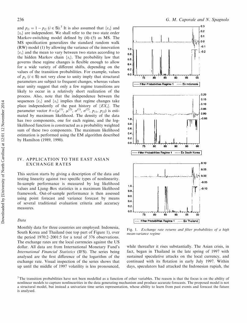
Data

Monthly data for three countries are employed: Indonesia,South Korea and Thailand (see top part of Figure 1), overthe period 1970:2–2001:5 for a total of 376 observations.The exchange rates are the local currencies against the USdollar. All data are from International Monetary Fund’sInternational Financial Statistics (IFS). The series beinganalysed are the first difference of the logarithm of theexchange rate. Visual inspection of the series shows thatup until the middle of 1997 volatility is less pronounced,

while thereafter it rises substantially. The Asian crisis, in

fact, began in Thailand in the late spring of 1997 with

sustained speculative attacks on the local currency, and

continued with its flotation in early July 1997. Within

days, speculators had attacked the Indonesian rupiah, the

3 The transition probabilities have not been modelled as a function of other variables. The reason is that the focus is on the ability ofnonlinear models to capture nonlinearities in the data generating mechanism and produce accurate forecasts. The proposed model is nota structural model, but instead a univariate time series representation, whose ability to learn from past events and forecast the futureis analysed.

Fig. 1. Exchange rate returns and filter probabilities of a highmean-variance regime

236 G. M. Caporale and N. Spagnolo

Dow

nloa

ded

by [

Uni

vers

ity o

f N

orth

Car

olin

a] a

t 12:

01 1

2 N

ovem

ber

2014

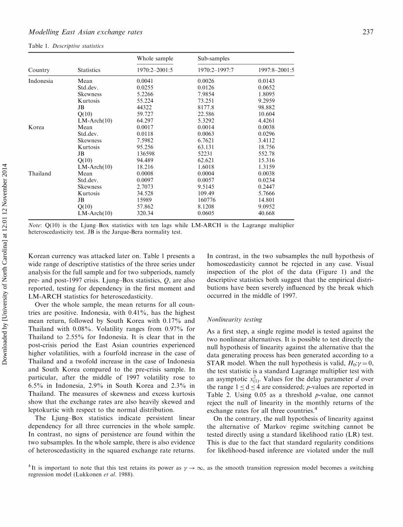
Korean currency was attacked later on. Table 1 presents a

wide range of descriptive statistics of the three series under

analysis for the full sample and for two subperiods, namely

pre- and post-1997 crisis. Ljung–Box statistics, Q, are also

reported, testing for dependency in the first moment and

LM-ARCH statistics for heteroscedasticity.

Over the whole sample, the mean returns for all coun-

tries are positive. Indonesia, with 0.41%, has the highest

mean return, followed by South Korea with 0.17% and

Thailand with 0.08%. Volatility ranges from 0.97% for

Thailand to 2.55% for Indonesia. It is clear that in the

post-crisis period the East Asian countries experienced

higher volatilities, with a fourfold increase in the case of

Thailand and a twofold increase in the case of Indonesia

and South Korea compared to the pre-crisis sample. In

particular, after the middle of 1997 volatility rose to

6.5% in Indonesia, 2.9% in South Korea and 2.3% in

Thailand. The measures of skewness and excess kurtosis

show that the exchange rates are also heavily skewed and

leptokurtic with respect to the normal distribution.

The Ljung–Box statistics indicate persistent linear

dependency for all three currencies in the whole sample.

In contrast, no signs of persistence are found within the

two subsamples. In the whole sample, there is also evidence

of heteroscedasticity in the squared exchange rate returns.

In contrast, in the two subsamples the null hypothesis ofhomoscedasticity cannot be rejected in any case. Visualinspection of the plot of the data (Figure 1) and thedescriptive statistics both suggest that the empirical distri-butions have been severely influenced by the break whichoccurred in the middle of 1997.

Nonlinearity testing

As a first step, a single regime model is tested against thetwo nonlinear alternatives. It is possible to test directly thenull hypothesis of linearity against the alternative that thedata generating process has been generated according to aSTAR model. When the null hypothesis is valid, H0:�¼ 0,the test statistic is a standard Lagrange multiplier test withan asymptotic x2ð1Þ. Values for the delay parameter d overthe range 1� d� 4 are considered; p-values are reported inTable 2. Using 0.05 as a threshold p-value, one cannotreject the null of linearity in the monthly returns of theexchange rates for all three countries.4

On the contrary, the null hypothesis of linearity againstthe alternative of Markov regime switching cannot betested directly using a standard likelihood ratio (LR) test.This is due to the fact that standard regularity conditionsfor likelihood-based inference are violated under the null

4 It is important to note that this test retains its power as � ! 1, as the smooth transition regression model becomes a switchingregression model (Lukkonen et al. 1988).

Table 1. Descriptive statistics

Whole sample Sub-samples

Country Statistics 1970:2–2001:5 1970:2–1997:7 1997:8–2001:5

Indonesia Mean 0.0041 0.0026 0.0143Std.dev. 0.0255 0.0126 0.0652Skewness 5.2266 7.9854 1.8095Kurtosis 55.224 73.251 9.2959JB 44322 8177.8 98.882Q(10) 59.727 22.586 10.604LM-Arch(10) 64.297 5.3292 4.4261

Korea Mean 0.0017 0.0014 0.0038Std.dev. 0.0118 0.0063 0.0296Skewness 7.5982 6.7621 3.4112Kurtosis 95.256 63.131 18.756JB 136598 52231 552.78Q(10) 94.489 62.621 15.316LM-Arch(10) 18.216 1.6018 1.3159

Thailand Mean 0.0008 0.0004 0.0038Std.dev. 0.0097 0.0057 0.0234Skewness 2.7073 9.5145 0.2447Kurtosis 34.528 109.49 5.7666JB 15989 160776 14.801Q(10) 57.862 8.1208 9.0952LM-Arch(10) 320.34 0.0605 40.668

Note: Q(10) is the Ljung–Box statistics with ten lags while LM-ARCH is the Lagrange multiplierheteroscedasticity test. JB is the Jarque-Bera normality test.

Modelling East Asian exchange rates 237

Dow

nloa

ded

by [

Uni

vers

ity o

f N

orth

Car

olin

a] a

t 12:

01 1

2 N

ovem

ber

2014

hypothesis of linearity, as some parameters are unidentified

and scores are identically zero. However, appropriate test

procedures that overcome the former or both of these

difficulties do exist (Hansen, 1992, 1996; Garcia, 1998).

Hansen’s standardized likelihood ratio test is applied.

This procedure requires evaluation of the likelihood func-

tion across a grid of different values for the transition

probabilities and for each state-dependent parameter. The

value of the standardized likelihood ratio statistics and

related p-values under the null hypothesis (see Hansen,

1996, for details) provides strong evidence in favour of a

Markov mean-variance regime-switching specification for

all the countries.5 Given these results, next we compare the

in-sample and out-of-sample performance of a Markov

regime-switching model and a random walk specification.

Empirical results

The parameter estimates for Indonesia, South Korea and

Thailand together with standard errors, likelihood function

values and diagnostic statistics are presented in Table 3.

Specifically, we test for serial correlation, heteroscedasticity

and normality, in the standardized forecast residuals. The

two competing model residuals are also tested for neglected

nonlinearities. Table 3 reports the p-values of three nonli-

nearity tests, namely the RESET, the BDS and the Neural

test,6 under the null hypothesis that each of the three resi-

duals series is linear. The results confirm those obtained

using the Hansen test, namely it appears that for

Indonesia, South Korea and Thailand the simple random

walk hypothesis as in is not able to capture the features of

the data. There is clear evidence of serial correlation in the

levels, heteroscedasticity and non-normality (see Table 3).

Non-normality and the failure of the neglected nonlinearity

tests for the error term in Equation 1 motivate our use of

a Markov-switching mean-variance model.

In particular, the two-states Markov model (Equation 4)

is considered, where the process is allowed to switch

between two distributions, one corresponding to a low

volatility and the other to a high volatility sample. In par-

ticular, appreciation and depreciation of the local curren-

cies against the US dollar are modelled with volatility being

high during periods of crisis and low during periods of

stability. The likelihood values for this model are well

above the values that were obtained with the linear speci-

fication (see Table 3). The standard errors are all very

small, suggesting that both mean and variance are signifi-

cantly different in each regime. In particular, the high-

variance state is somewhere between 15 times (South

Korea) and 60 times (Indonesia) as volatile as the low-

variance state. Indeed, the two means and variances are

very different across regimes, being much higher in the

‘crisis’ regime than in the other one. In particular, in

the case of Indonesia, the standard deviation of returns

in the low volatility regime is equal to 0.0012 in the pre-

crisis period compared to 0.0740 in the highly volatile post-

crisis sample. The same general pattern emerges for South

Korea and Thailand (see Table 3). Based on the parameter

estimates of the high and low means and variances, the

filter probabilities can be estimated, which are the prob-

ability that each observation is in the high state or the

low state. As the filtering procedure of Hamilton (1990,

1994) shows, the sequence of past exchange rates contains

useful information for the identification of the current state

of the exchange rate. The filtered probabilities of a high

mean-variance state are displayed in the bottom part of

Figure 1. The separation into regimes is very clear-cut,

the probabilities being close to zero or one, and confirms

the impression given by visual inspection of the data. The

transition probabilities appear robust across regimes,

5Note that the two nonlinear models considered in the paper allow one to select the breakpoint endogenously rather than choosing ita priori and then modelling it with a dummy variable. The difference between the two approaches is substantial and makes the nonlinearapproach far more attractive and statistically correct. The point forecasts, in fact, will only depend on the breakpoints inferred from thedata rather that being arbitrarily chosen by the researcher.6 See Lee et al. (1993).

Table 2. Nonlinearity testing

Linearity against STAR model

Indonesia Korea Thailand

Delay1 2.2118 4.7197 4.9695

(0.3312) (0.0944) (0.0833)2 5.9191 2.4917 3.0256

(0.5113) (0.2878) (0.2203)3 6.8974 3.1174 6.1793

(0.0752) (0.3739) (0.1032)4 3.0677 1.7391 13.572

(0.3813) (0.6283) (0.0035)K 2 2 2

Linearity against Markov switching modelStandardized LR test

LR 8.9911 7.9415 8.7653M¼ 0 0.0001 0.0001 0.0001M¼ 1 0.0001 0.0001 0.0001M¼ 2 0.0001 0.0001 0.0001M¼ 3 0.0001 0.0001 0.0001M¼ 4 0.0001 0.0001 0.0001

Note: See Hansen (1996) for details of the test statistic, such as thedefinition of M. p-values are in parentheses. The selectionof the maximum lag order k of the AR was made using SBC.

238 G. M. Caporale and N. Spagnolo

Dow

nloa

ded

by [

Uni

vers

ity o

f N

orth

Car

olin

a] a

t 12:

01 1

2 N

ovem

ber

2014

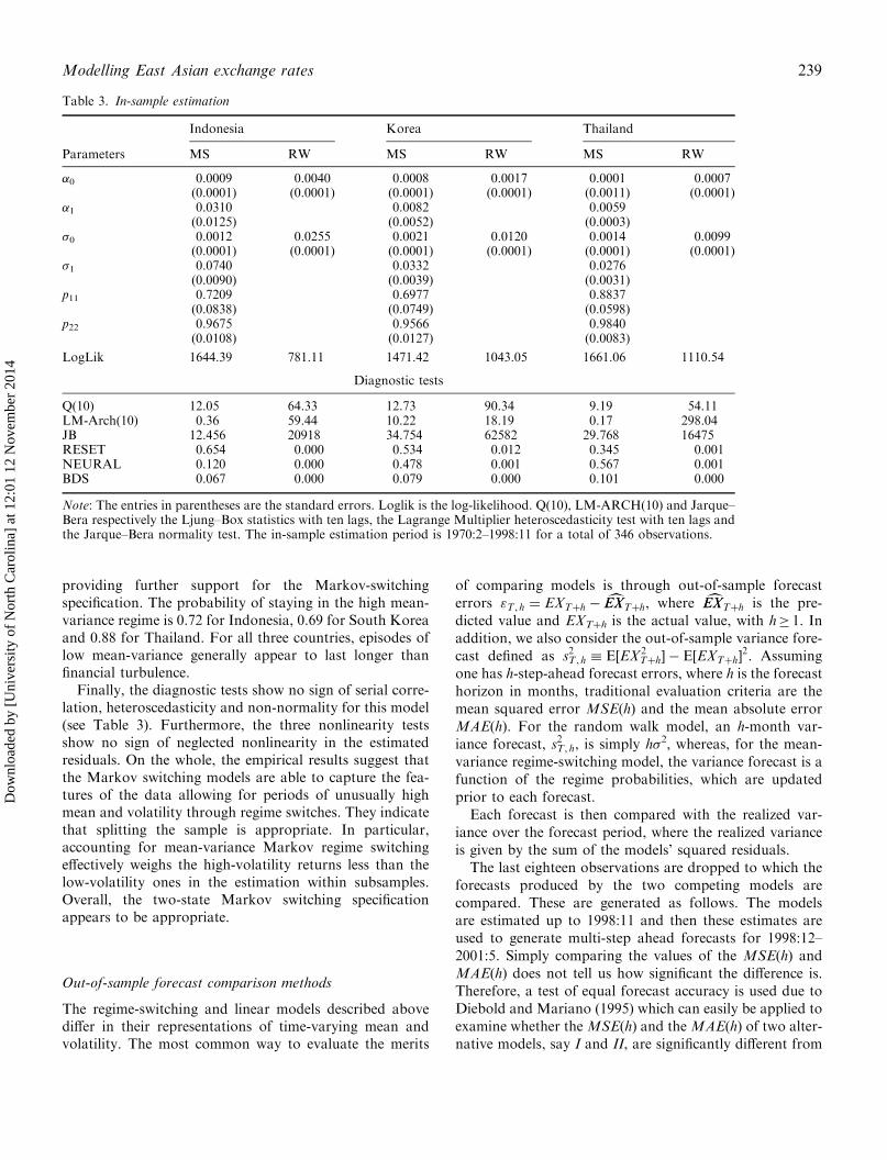
providing further support for the Markov-switchingspecification. The probability of staying in the high mean-variance regime is 0.72 for Indonesia, 0.69 for South Koreaand 0.88 for Thailand. For all three countries, episodes oflow mean-variance generally appear to last longer thanfinancial turbulence.

Finally, the diagnostic tests show no sign of serial corre-lation, heteroscedasticity and non-normality for this model(see Table 3). Furthermore, the three nonlinearity testsshow no sign of neglected nonlinearity in the estimatedresiduals. On the whole, the empirical results suggest thatthe Markov switching models are able to capture the fea-tures of the data allowing for periods of unusually highmean and volatility through regime switches. They indicatethat splitting the sample is appropriate. In particular,accounting for mean-variance Markov regime switchingeffectively weighs the high-volatility returns less than thelow-volatility ones in the estimation within subsamples.Overall, the two-state Markov switching specificationappears to be appropriate.

Out-of-sample forecast comparison methods

The regime-switching and linear models described abovediffer in their representations of time-varying mean andvolatility. The most common way to evaluate the merits

of comparing models is through out-of-sample forecast

errors "T , h ¼ EXTþh �cEXEXTþh, where cEXEXTþh is the pre-

dicted value and EXTþh is the actual value, with h� 1. In

addition, we also consider the out-of-sample variance fore-

cast defined as s2T , h � E½EX2Tþh� � E½EXTþh�

2. Assuming

one has h-step-ahead forecast errors, where h is the forecast

horizon in months, traditional evaluation criteria are the

mean squared error MSE(h) and the mean absolute error

MAE(h). For the random walk model, an h-month var-

iance forecast, s2T , h, is simply h�2, whereas, for the mean-

variance regime-switching model, the variance forecast is a

function of the regime probabilities, which are updated

prior to each forecast.

Each forecast is then compared with the realized var-

iance over the forecast period, where the realized variance

is given by the sum of the models’ squared residuals.

The last eighteen observations are dropped to which the

forecasts produced by the two competing models are

compared. These are generated as follows. The modelsare estimated up to 1998:11 and then these estimates are

used to generate multi-step ahead forecasts for 1998:12–

2001:5. Simply comparing the values of the MSE(h) and

MAE(h) does not tell us how significant the difference is.

Therefore, a test of equal forecast accuracy is used due to

Diebold and Mariano (1995) which can easily be applied to

examine whether the MSE(h) and theMAE(h) of two alter-

native models, say I and II, are significantly different from

Table 3. In-sample estimation

Indonesia Korea Thailand

Parameters MS RW MS RW MS RW

�0 0.0009 0.0040 0.0008 0.0017 0.0001 0.0007(0.0001) (0.0001) (0.0001) (0.0001) (0.0011) (0.0001)

�1 0.0310 0.0082 0.0059(0.0125) (0.0052) (0.0003)

�0 0.0012 0.0255 0.0021 0.0120 0.0014 0.0099(0.0001) (0.0001) (0.0001) (0.0001) (0.0001) (0.0001)

�1 0.0740 0.0332 0.0276(0.0090) (0.0039) (0.0031)

p11 0.7209 0.6977 0.8837(0.0838) (0.0749) (0.0598)

p22 0.9675 0.9566 0.9840(0.0108) (0.0127) (0.0083)

LogLik 1644.39 781.11 1471.42 1043.05 1661.06 1110.54

Diagnostic tests

Q(10) 12.05 64.33 12.73 90.34 9.19 54.11LM-Arch(10) 0.36 59.44 10.22 18.19 0.17 298.04JB 12.456 20918 34.754 62582 29.768 16475RESET 0.654 0.000 0.534 0.012 0.345 0.001NEURAL 0.120 0.000 0.478 0.001 0.567 0.001BDS 0.067 0.000 0.079 0.000 0.101 0.000

Note: The entries in parentheses are the standard errors. Loglik is the log-likelihood. Q(10), LM-ARCH(10) and Jarque–Bera respectively the Ljung–Box statistics with ten lags, the Lagrange Multiplier heteroscedasticity test with ten lags andthe Jarque–Bera normality test. The in-sample estimation period is 1970:2–1998:11 for a total of 346 observations.

Modelling East Asian exchange rates 239

Dow

nloa

ded

by [

Uni

vers

ity o

f N

orth

Car

olin

a] a

t 12:

01 1

2 N

ovem

ber

2014

each other. The loss differential, dT (h), for the h-step fore-cast is

dT ðhÞ ¼ ð"IT , hÞ2� ð"IIT , hÞ

2ð7Þ

for the MSE(h) and

dT ðhÞ ¼ "IT , h

�� ��� "IIT , h

�� �� ð8Þ

for the MAE(h). The null hypothesis of equal forecastaccuracy is E(dT (h))¼ 0.

Another useful criterion which is widely applied in eval-uations of ex-post forecasts is Theil’s inequality coefficient(Theil, 1966), defined as

UðhÞ ¼

ffiffiffiffiffiffiffiffiffiffiffiffiffiffiffiffiffiffiffiffiffiffiffiffiffiffiffiffiffiffiffiffiffiffiffiffiffiffiffiffiffið1=hÞðxTþh � xxTþhÞ

2q

ffiffiffiffiffiffiffiffiffiffiffiffiffiffiffiffiffiffiffiffiffiffiffiffiffiffið1=hÞðxTþhÞ

2q ð9Þ

where xTþh ¼ ð"T , h, s2T , hÞ and h is the number of periods

being forecasted. The scaling of the numerator/denomi-nator is such that U(h) will always fall between 0 and 1.If UðhÞ ¼ 0, xTþh ¼ xxTþh and there is a perfect predic-tion. On the other hand, when U(h)¼ 1 the predictiveperformance of the model is as bad as it could be.

Forecast comparisons are made in the following way.Each time series is composed of Tþh observations, andthe first T observations are used to estimate the linear andnonlinear models. In the two and half years out-of-sampleperiod (from 1998:12 to 2001:5) there are 30 monthsto predict. We generate from all the estimated models 1 toh-step-ahead forecasts. The forecast horizon h has been setequal to 12. A strategy of sequential estimation is employedby rolling over the sample one period at time andhence constructing different forecast series (18) for each

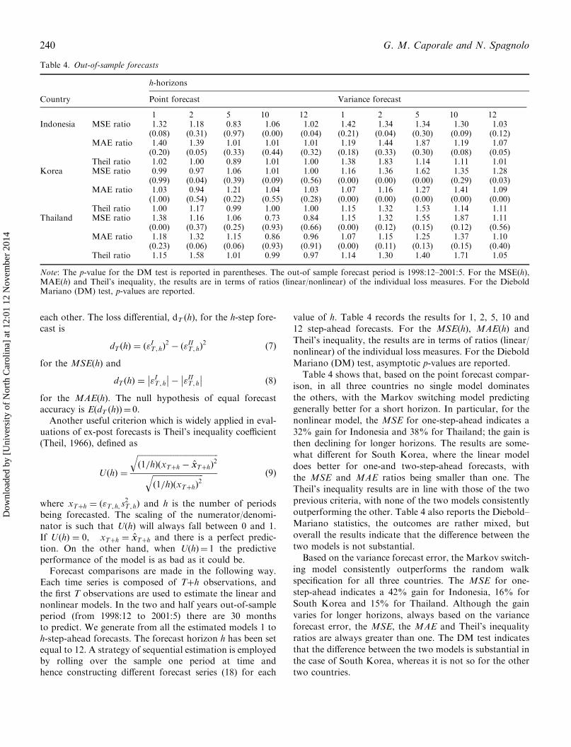
value of h. Table 4 records the results for 1, 2, 5, 10 and

12 step-ahead forecasts. For the MSE(h), MAE(h) and

Theil’s inequality, the results are in terms of ratios (linear/

nonlinear) of the individual loss measures. For the Diebold

Mariano (DM) test, asymptotic p-values are reported.

Table 4 shows that, based on the point forecast compar-

ison, in all three countries no single model dominates

the others, with the Markov switching model predicting

generally better for a short horizon. In particular, for the

nonlinear model, the MSE for one-step-ahead indicates a

32% gain for Indonesia and 38% for Thailand; the gain is

then declining for longer horizons. The results are some-

what different for South Korea, where the linear model

does better for one-and two-step-ahead forecasts, with

the MSE and MAE ratios being smaller than one. The

Theil’s inequality results are in line with those of the two

previous criteria, with none of the two models consistently

outperforming the other. Table 4 also reports the Diebold–

Mariano statistics, the outcomes are rather mixed, but

overall the results indicate that the difference between the

two models is not substantial.

Based on the variance forecast error, the Markov switch-

ing model consistently outperforms the random walk

specification for all three countries. The MSE for one-

step-ahead indicates a 42% gain for Indonesia, 16% for

South Korea and 15% for Thailand. Although the gain

varies for longer horizons, always based on the variance

forecast error, the MSE, the MAE and Theil’s inequality

ratios are always greater than one. The DM test indicates

that the difference between the two models is substantial in

the case of South Korea, whereas it is not so for the other

two countries.

Table 4. Out-of-sample forecasts

h-horizons

Country Point forecast Variance forecast

1 2 5 10 12 1 2 5 10 12Indonesia MSE ratio 1.32 1.18 0.83 1.06 1.02 1.42 1.34 1.34 1.30 1.03

(0.08) (0.31) (0.97) (0.00) (0.04) (0.21) (0.04) (0.30) (0.09) (0.12)MAE ratio 1.40 1.39 1.01 1.01 1.01 1.19 1.44 1.87 1.19 1.07

(0.20) (0.05) (0.33) (0.44) (0.32) (0.18) (0.33) (0.30) (0.08) (0.05)Theil ratio 1.02 1.00 0.89 1.01 1.00 1.38 1.83 1.14 1.11 1.01

Korea MSE ratio 0.99 0.97 1.06 1.01 1.00 1.16 1.36 1.62 1.35 1.28(0.99) (0.04) (0.39) (0.09) (0.56) (0.00) (0.00) (0.00) (0.29) (0.03)

MAE ratio 1.03 0.94 1.21 1.04 1.03 1.07 1.16 1.27 1.41 1.09(1.00) (0.54) (0.22) (0.55) (0.28) (0.00) (0.00) (0.00) (0.00) (0.00)

Theil ratio 1.00 1.17 0.99 1.00 1.00 1.15 1.32 1.53 1.14 1.11Thailand MSE ratio 1.38 1.16 1.06 0.73 0.84 1.15 1.32 1.55 1.87 1.11

(0.00) (0.37) (0.25) (0.93) (0.66) (0.00) (0.12) (0.15) (0.12) (0.56)MAE ratio 1.18 1.32 1.15 0.86 0.96 1.07 1.15 1.25 1.37 1.10

(0.23) (0.06) (0.06) (0.93) (0.91) (0.00) (0.11) (0.13) (0.15) (0.40)Theil ratio 1.15 1.58 1.01 0.99 0.97 1.14 1.30 1.40 1.71 1.05

Note: The p-value for the DM test is reported in parentheses. The out-of sample forecast period is 1998:12–2001:5. For the MSE(h),MAE(h) and Theil’s inequality, the results are in terms of ratios (linear/nonlinear) of the individual loss measures. For the DieboldMariano (DM) test, p-values are reported.

240 G. M. Caporale and N. Spagnolo

Dow

nloa

ded

by [

Uni

vers

ity o

f N

orth

Car

olin

a] a

t 12:

01 1

2 N

ovem

ber

2014

V. CONCLUSIONS

This study has investigated the ability of mean-variance

regime-switching models to capture the time series proper-

ties of exchange rate series that have been subject to a

severe depreciation. Monthly data have been employed

on the local currencies against the US dollar for three

countries, Indonesia, South Korea and Thailand, over the

period 1970:1–2001:5. The crisis which occurred in East

Asia in 1997 led to a massive depreciation of these curren-

cies and represented a major regime shift. As the analysis

shows, standard random walk models are not able to take

into account the structural break which occurred in the

data generating process. Instead, it is more appropriate,

under these circumstances, to employ a Markov regime-

switching model that allows for discrete shifts in the

mean and variance. Such a specification, in fact, provides

a better fit to the data than the competing models, and

captures well the features of the series. The estimated

Markov switching model passes all the diagnostic tests

and provides a satisfactory description of the nonlinearities

found in the data. The results show that there is persistence

of the two states, with the regime characterized by less

volatility exhibiting more persistence. As for the out-

of-sample point forecast results, no single model seems to

completely dominate the others. However, the insults indi-

cate that the mean-variance Markov switching model

reduces the variance forecast error relative to the linear

model. A possible explanation is that the difference

between the two regimes can mainly be put down to a

shift in volatility rather than in the mean, the former not

being taken into account by the point forecast criteria. On

the whole, these results can be interpreted as being consis-

tent with the multiple-equilibrium approach to currency

crises, which emphasizes the role of self-fulfilling expecta-

tions as opposed to fundamentals in explaining crises. In

fact, as shown by Jeanne and Masson (2000), an empirical

model of the type that has been estimated can be seen as a

linearized reduced form of a structural model with multiple

equilibria and sudden jumps from one equilibrium to

another. Surprisingly, to date no empirical studies had

used this framework to model exchange rates in emerging

economies. Our contribution fills this gap.

ACKNOWLEDGEMENTS

Financial assistance from Leverhulme grant F/711/A,

‘Volatility of share prices and the macroeconomy: real

effects of financial crises’, is gratefully acknowledged. We

are also grateful to an anonymous referee and to partici-

pants at the 2000 MMF Meeting, London, 6–8 September

2000, for useful comments.

REFERENCES

Bacon, D. W. and Watts, D. G. (1971) Estimating the transitionbetween two intersecting straight lines, Biometrika, 58,525–34.

Bekaert, C. and Hodrick, R. J. (1993) On biases in the measure-ment of foreign exchange risk premium, Journal ofInternational Money and Finance, 12, 115–38.

Chan, K. S. and Tong, H. (1986) On estimating thresholds inautoregressive models, Journal of Time Series Analysis, 7,179–90.

Corbett, J. and Vines, D. (1999) Asian currency and financialcrises: lessons from vulnerability, crises and collapse, in TheAsian Financial Crises: Causes, Contagion and Consequences(Eds) P. R. Agenos, M. Miller, D. Vines and A. Weber,Cambridge University Press, Cambridge.

Corsetti, G., Pesenti, P. and Roubini, N. (1999) The Asian crisis:an overview of the empirical evidence and policy debate,in The Asian Financial Crises: Causes, Contagion, andConsequences (Eds) P. R. Agenor, M. Miller, D. Vines andA. Weber, Cambridge University Press, Cambridge, pp. 127–163.

De Gooijer, J. G. and Kumar, K. (1992) Some recent develop-ments in nonlinear time series modeling, testing and forecast-ing, International Journal of Forecasting, 8, 135–56.

Diebold, F. X. and Mariano, R. S. (1995) Comparing predictiveaccuracy, Journal of Business and Economic Statistics, 13,253–63.

Diebold, F. X. and Nason, J. A. (1990) Nonparametric exchangerate prediction, Journal of International Economics, 28,315–22.

Engel, C. (1994) Can the Markov switching model forecastexchange rates?, Journal of International Economics, 36,151–65.

Engel, C. and Hakkio, K. (1997) The distribution of exchangerates in the EMS, International Journal of Finance andEconomics, 33, 15–32.

Engel, C. and Hamilton, J. D. (1990) Long swings in the dollar:are they in the data and do the markets know it?, AmericanEconomic Review, 80, 689–713.

Frankel, J. A. and Rose, A. K. (1994) A survey of empiricalresearch on nominal exchange rates, NBER Working Paper,4865.

Garcia, R. (1998) Asymptotic null distribution of the likelihoodratio test in Markov switching models, InternationalEconomic Review, 39, 763–88.

Granger, C. W. J. and Terasvirta, T. (1993) Modelling NonlinearEconomic Relationships, Oxford University Press, Oxford.

Hamilton, J. D. (1988) Rational expectations econometric analy-sis of changes in regime: an investigation of the term struc-ture of interest rates, Journal of Economic Dynamics andControl, 12, 385–423.

Hamilton, J. D. (1989) A new approach to the economic analy-sis of nonstationary time series and the business cycle,Econometrica, 57, 357–84.

Hamilton, J. D. (1990) Analysis of time series subject to changesin regime, Journal of Econometrics, 45, 39–70.

Hamilton, J. D. (1994) Time Series Analysis, Princeton UniversityPress, Princeton, NJ.

Hansen, B. E. (1992) The likelihood ratio test undernonstandard conditions: testing the Markov switchingmodel of GNP, Journal of Applied Econometrics, 7, 61–82.

Hansen, B. E. (1996) Erratum: The likelihood ratio testunder nonstandard conditions: testing the Markovswitching model of GNP, Journal of Applied Econometrics,11, 195–8.

Modelling East Asian exchange rates 241

Dow

nloa

ded

by [

Uni

vers

ity o

f N

orth

Car

olin

a] a

t 12:

01 1

2 N

ovem

ber

2014

Hsieh, D. A. (1989) Testing for nonlinear dependence in foreignexchange rate, Journal of Business, 62, 339–68.

Jeanne, O. and Masson, P. (2000) Currency crises, sunspotsand Markov-switching regimes, Journal of InternationalEconomics, 50, 327–50.

Krugman, P. (1991) Target zones and exchange rate dynamics,Quarterly Journal of Economics, 106, 669–82.

Lee, T.-H., White, H. and Granger, C. W. J. (1993) Testing forneglected nonlinearity in time series models: a comparisonof neural network methods and alternative tests, Journalof Econometrics, 56, 269–90.

Lukkonen, R., Saikkonen, P. and Terasvirta, T. (1988) Testinglinearity against smooth transition autoregressive models,Biometrika, 75, 491–9.

Meese, R. A. and Rogoff, K. (1983) Empirical exchange ratemodels of the seventies: do they fit out of sample?, Journalof International Economics, 14, 3–12.

Meese, R. A. and Rose, A. K. (1990) Nonlinear, nonparametric,nonessential exchange rate estimation, The AmericanEconomic Review, 80, 192–6.

Obstfeld, M. (1996) Models of currency crises with self-fulfillingfeatures, European Economic Review, 40, 1037–47.

Sarantis, N. (1999) Modeling non-linearities in real effectiveexchange rates, Journal of International Money and Finance,18, 27–45.

Stock, J. H. (1987) Measuring business cycle time, Journal ofPolitical Economy, 95, 132–54.

Taylor, M. P. and Peel, D. A. (2000) Nonlinear adjustment, long-run equilibrium and exchange rate fundamentals, Journal ofInternational Money and Finance, 19, 33–53.

Theil, H. (1966) Applied Economic Forecasts, North-Holland,Amsterdam.

242 G. M. Caporale and N. Spagnolo

Dow

nloa

ded

by [

Uni

vers

ity o

f N

orth

Car

olin

a] a

t 12:

01 1

2 N

ovem

ber

2014