modelling commodities for counterparty risk...

Modelling Commodities for Counterparty Risk Calculations

10 October 2012

Vinay KotechaVladimir Chorniy

Risk Methodology & Analytics

Group Risk Management

BNP Paribas

Quant Congress Europe 2012

Quant Congress 2012 2

Agenda

• Commodities Market

• Computing counterparty risk on commodity products

• Choosing a model: stylised features of the market

• Model in practice: correlation and calibration

• Simulation results

Quant Congress 2012

Map of Risk Quant - Real World Measure (a fragment)

LEM RegC CVA PFE

Exposure on defaultCorrelation (contagion) of default events (including reference entity) and market risk factorsConditionality on default vs. correlation/co-dependence of factors

Multiple assets modelling(“super hybrid”) stable and consistent

Sub-optimal exercise – PFE, CVAInstruments (e.g. Bermudan)Early termination agreements (ETO)Real world specials: Inflation,

Stochastic volatility (implied and realised),

Stochastic commodity including power

Predictors: variance and expectations

Dynamics of realised and forward asset values

Limitations of stochastic process(pricing vs. real world)

How to build real world asset modelHow to calibrate real world asset model

Limitation of methodsFast pricers, sparse data

Limitation of methodsAMC

Hedging CVA strategyCVA links to real world of cost:relation to EL, EC, funding cost,CVA as profitably measure(s)

3

Quant Congress 2012

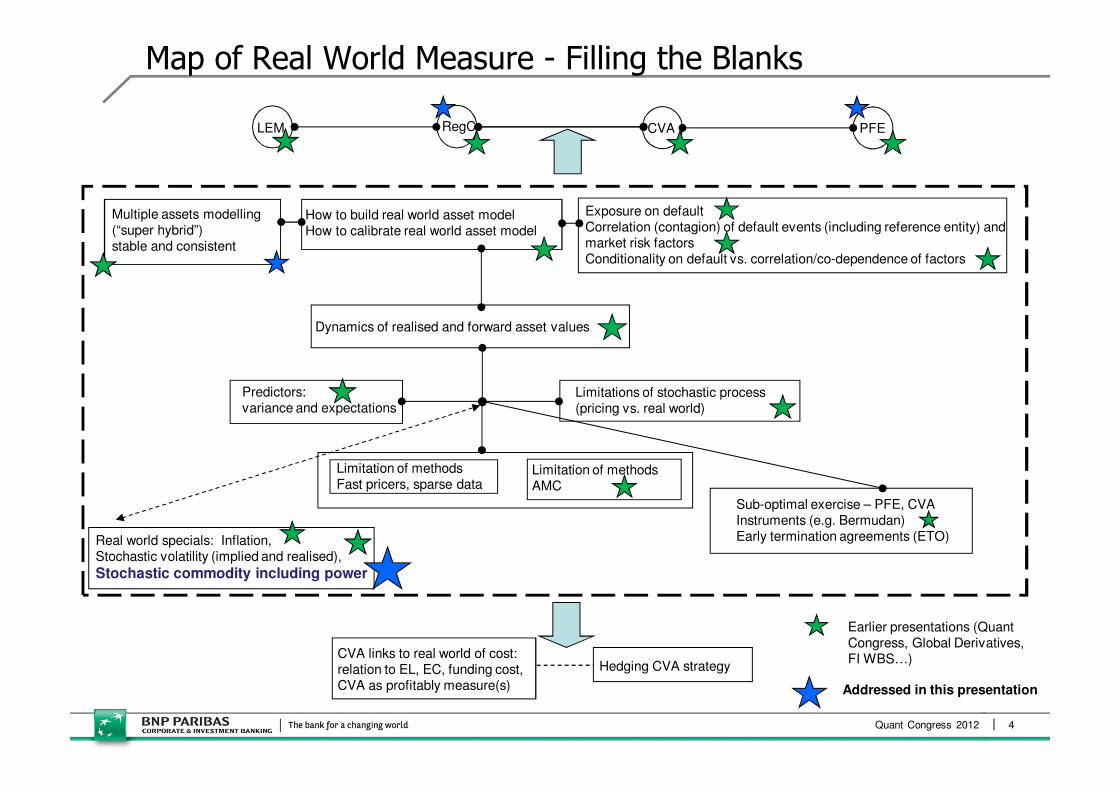
Map of Real World Measure - Filling the Blanks

LEM RegC CVA PFE

Exposure on defaultCorrelation (contagion) of default events (including reference entity) and market risk factorsConditionality on default vs. correlation/co-dependence of factors

Multiple assets modelling(“super hybrid”) stable and consistent

Sub-optimal exercise – PFE, CVAInstruments (e.g. Bermudan)Early termination agreements (ETO)Real world specials: Inflation,

Stochastic volatility (implied and realised),

Stochastic commodity including power

Predictors: variance and expectations

Dynamics of realised and forward asset values

Limitations of stochastic process(pricing vs. real world)

How to build real world asset modelHow to calibrate real world asset model

Limitation of methodsFast pricers, sparse data

Limitation of methodsAMC

Addressed in this presentation

Hedging CVA strategyCVA links to real world of cost:relation to EL, EC, funding cost,CVA as profitably measure(s)

Earlier presentations (Quant Congress, Global Derivatives, FI WBS…)

4


Background on Commodity Markets

• Major commodity markets:

� Energy: Crude Oil, Crack Products, Natural Gas, Coal, Electricity, …

� Base Metals: Copper, Aluminium, Zinc, …

� Agriculture: Wheat, Corn, Soybeans, …

� Freight: Clean, Dirty Tanker Routes, …

� Environmental: EU, UN Emission Rights, …

• Commonly traded products

� Predominately vanilla: financial swaps, basis swaps (calendar and crack), vanilla and asian options: both single period and monthly (averaged) strips

� Typical exotics include: crack or spark spread options, barriers, extendible swaps, gas storage, park & loan, etc

• Spot is not actively traded except in some markets, e.g. electricity

• Physical underlying is rarely traded by financial institutions

� Modelling physical can be complex as we need to consider storage costs, convenience yields, specific grades, etc


A Quick Primer on Risk Management

• Quantitative risk management encompasses models for the calculation of

� Market risk (e.g. Value at Risk)

� Counterparty exposure (closely related to CVA)

• Both involve the simulation of market variables using the real-world measureand a revaluation of positions

• Both focus on high percentiles

• Both affect regulatory capital

• Desirable model features:

� We want to correctly model the evolution of market variables

� We want to be able to accurately price products

� For exposure predictions this needs to be done to long time horizons

� Need to ensure risk factors are cross-correlated (potentially thousands)

� Also need to incorporate wrong-way or right-way effects

• Focus here is on scenario generation model for counterparty exposure calculation


Calculating Counterparty Credit Exposure

• Counterparty credit risk is linked to the replacement cost of a derivative in the event the counterpart defaults

� Measured by computing the potential future values of the derivative

• The potential future value of the derivative can result in exposure: positive values generate exposure as counterparts owe us; negative values generate

no exposure

• Typically, PFE on a derivative is computed using a Monte-Carlo simulation:

Step 1: simulate possible future evolution of the market parameters or ‘risk drivers’, e.g., commodity prices, spot FX, at various time-points

Step 2: calculate the future value of the transaction at each time-point under each future market scenario

Step 3: calculate the required measure from the distribution of deal PVs

• Various measures can be computed from the distribution of future deal PVs:

� high percentiles (e.g. 95th) for limit monitoring; effective expected positive exposure for regulatory capital; expected exposure for CVA


PFE Modelling - High-level Requirements from a Model

• Model should capture the right behaviour of commodities

� For Front Office (or pricing) needs are well understood: the primary requirement is that model matches market prices and allows for good hedging

� What is considered ‘right behaviour’ for counterparty risk?

� Require simulations to be in line with historically observed behaviour

• Model should be able to capture long-term behaviour of commodity forward curves

� At the same time, we need to pay attention to corresponding short term dynamics of prices, for example over 10 or 20 days: this is the driver of risk for trades under Credit Support Annexe (CSA)

• Ensure model captures the stylised features of the commodity markets

• Ideally require one model suitable for use across a range of commodity markets, both for storable and non-storable types

� Stick to reduced-form (exogenous) models over structural (endogenous) models. The latter for instance aim to capture price behaviour through modelling of the production processes themselves

� Calibration should be in the real-world measure


Stylised Features of the Market I

• How to choose a model for counterparty risk purposes?

• Rely on stylised features of the commodity markets

� Empirical analysis shows that there are a number of key features in the behaviour of commodity prices

1. Changing shape of the futures curves: the backwardation-contango duality

� Futures curves (non-seasonal) tend to be either in backwardation or contango

� This shape can change over time. For example, Brent crude oil futures curve was in backwardation on 03/10/2011, and in contango on 18/10/2010

� A multi-factor model is required to capture this effect in the simulations

2. Capture mean reversion:

� Tendency of prices to bounce back to long-term “average”

� Determined by cost of production; deviations are linked to supply and demand constraints

� Mean-reversion is linked to downward sloping volatility term-structure: volatility of short maturity futures is generally higher than long term maturities


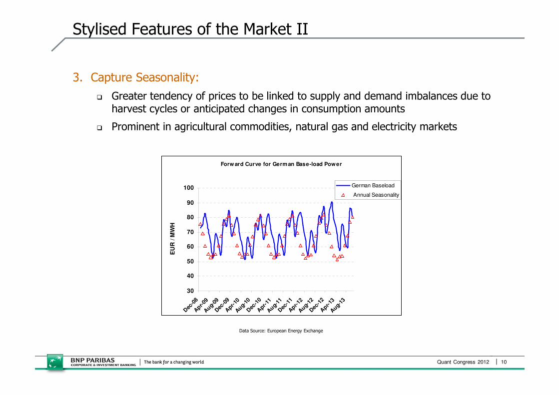
Stylised Features of the Market II

3. Capture Seasonality:

� Greater tendency of prices to be linked to supply and demand imbalances due to harvest cycles or anticipated changes in consumption amounts

� Prominent in agricultural commodities, natural gas and electricity markets

Forw ard Curve for German Base-load Power

30

40

50

60

70

80

90

100

Dec

-08

Apr-

09A

ug-09

Dec

-09

Apr-

10A

ug-10

Dec

-10

Apr-

11A

ug-11

Dec

-11

Apr-

12A

ug-12

Dec

-12

Apr-

13A

ug-13

EU

R / M

WH

German Baseload

Annual Seasonality

Data Source: European Energy Exchange


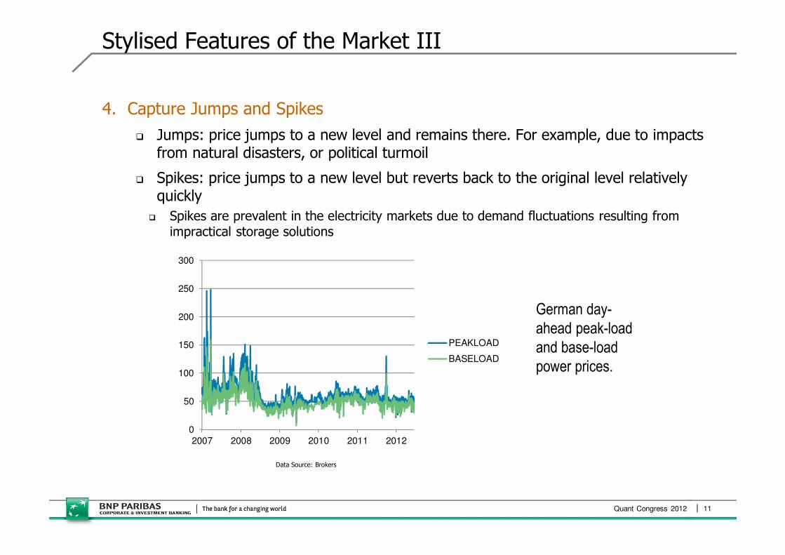
Stylised Features of the Market III

4. Capture Jumps and Spikes

� Jumps: price jumps to a new level and remains there. For example, due to impacts from natural disasters, or political turmoil

� Spikes: price jumps to a new level but reverts back to the original level relatively quickly

� Spikes are prevalent in the electricity markets due to demand fluctuations resulting from impractical storage solutions

German day-

ahead peak-load

and base-load

power prices.

0

50

100

150

200

250

300

2007 2008 2009 2010 2011 2012

PEAKLOAD

BASELOAD

Data Source: Brokers


Stylised Features of the Market IV

5. Capture regional idiosyncrasies of the market

� For example, US natural gas and power trading is very regional

� Main hubs are actively traded but most other pipelines traded at a spread to the Hubs

� For example, Louisiana, Texas HSC, Oklahoma are margined to Henry Hub

• Hubs versus pipeline gas prices tend to be co-integrated in the long term

� From modelling perspective, is it better to model the price of the pipeline or the spread?

Henry Hub

Nymex Fixing

RockiesCig

Sumas

CanadaAeco

EmpressAppalachian

Chicago

Colgas

OklahomaPanhand

Ventura

LouisianaTenn/La

TexasHsc

TetcWest

TexasEl Paso


Commodity Models in Literature

• There are numerous commodity models in the literature

• Models fall into two main classes:

� Spot-based models: for example Schwartz (1997), Gibson & Schwartz (1990)

� Forward-based models: Clewlow-Strickland (1999), Crosby (2006)

• From a counterparty risk calculation perspective, there are advantages and drawbacks with both frameworks

� For spot-based models:

� simulation is more tractable

� however, difficult to construct the exact initial market observed forward curve

� no-arbitrage relation between spot prices and forward price no longer valid

� For forward-based models:

� initial market observed forward curve is an input to the model

� simulation is less tractable

� these models rely, heavily, on a large data set

• Required to match the simulation time zero forward curve, so that PVs can match front office PVs, and the simulated collateral calculation is accurate

� Multi-factor spot models provide some control over forward curve (e.g. via convenience yield), but are typically not sufficient to match a forward curve with periodic seasonal structure

• This leads to the choice of a model of the forward curve. The extended Clewlow-Strickland (1999) model using two factors is chosen to capture the change in shape of forward curve over time

� The functional form of the volatility is the following:

� Explicit specification of the functional form improves analytic tractability – important for obtaining a fast Monte-Carlo simulation – and provides a means to constrain the calibration where required


Model Choice – ‘Primary’ Commodities

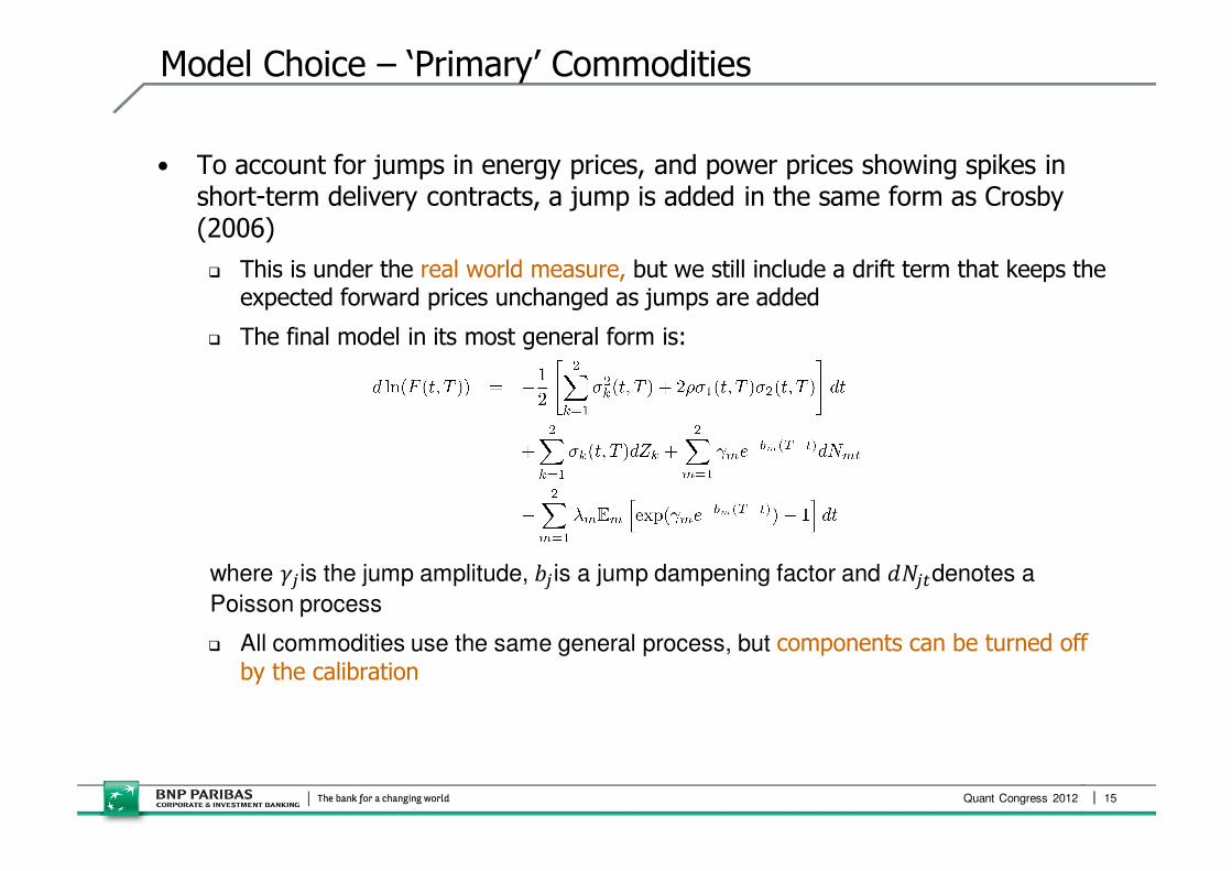
• To account for jumps in energy prices, and power prices showing spikes in short-term delivery contracts, a jump is added in the same form as Crosby (2006)

� This is under the real world measure, but we still include a drift term that keeps the expected forward prices unchanged as jumps are added

� The final model in its most general form is:

where ��is the jump amplitude, ��is a jump dampening factor and ��denotes a

Poisson process

� All commodities use the same general process, but components can be turned off

by the calibration


Model Choice – ‘Primary’ Commodities

Quant Congress 2012

Model Choice – Interdependence of Jumps & Spikes

• In the power markets, empirically, we see that if a spike occurs in one market then neighbouring markets are also influenced

� For example, if German Peak-load electricity (power) price spikes then French and Dutch Peak-load prices are influenced as well

� Chart and table below illustrates the distribution of German, French and Dutch peak-load spikes

� Spike here is defined as a daily move in price over 2 standard deviations

% Move over 2 standard deviations in Price for German, French

and Dutch Peak-load Power

0%

100%

200%

300%

400%

500%

600%

700%

800%

06-Oct-03 17-Feb-05 02-Jul-06 14-Nov-07 28-Mar-09

German

French

Dutch

Chart showing the distribution of moves (up and down) over 2

standard deviations for German, French and Dutch power markets:

Table illustrating the number of simultaneous

jump events for 3 Euro power markets as a

function of standard deviations:


• Given markets jump (or spike) together, what are the sizes of jumps in the various markets?

• Tables below illustrate the behaviour of price jumps in ‘neighbouring’ markets given a jump in one market:

� Consider the concept of a ‘driving’ market and a ‘neighbour’ market

• When a >2 std dev move occurs in one market, the probability of >1 std devmove is large in neighbouring markets

� Consider splitting the jump into a systemic and an idiosyncratic component


Tables illustrating the

behaviour of jump events of

neighbouring markets given a

large move is observed for

the ‘driving’ market

• Practically, to capture the ‘co-dependence’, jumps are modelled via two separate Poisson processes, one ‘systemic’ and another ‘idiosyncratic’

� Commodities which are known to jump together are grouped together and assigned the ‘systemic’ Poisson process

� Empirical (or fundamental market) analysis motivates which commodities are grouped together

� Arrival times for all commodities belonging to the ‘systemic’ process are the same

� There can be multiple systemic jump configurations: for example, a group for EURO Gas & Power, US Gas & Power, Crude Oil & Refined, etc

• At each universe and simulation time-point, the ‘driving market’ is randomly sampled from the group of commodities for the ‘systemic’ process

� The driving market has the largest jump size; the neighbour markets jump with a fixed ratio to the driving markets

� These ratios are empirically determined

� Under this set-up, the jump sizes are fixed (non-stochastic), although this assumption can be relaxed

� Idiosyncratic are non-propagating, unique to the assigned commodity or region




Example Simulation Envelopes

• Simulation envelopes (10,000 simulations). Effect of downward sloping volatility term structure leads to the mean reversion – flattening of the envelopes for Fuel Oil:

0

100

200

300

400

500

0 10 20 30

EU

R

Years

99%

90%

10%

1%

50%

Mean


Example Forward Curve Simulation Envelope

• 90th/10th percentile simulation envelopes for Euro Base-load power forward curve. The effects of spikes (jumps) can be seen in the short end delivery. The exponential jump dampening term ensures long end of the curve is unaffected.

ValRisk Tenor 6 Months

-

20

40

60

80

100

120

140

160

180

200

1D 3D 5D 1W 1M 3M 5M 7M 9M 11M

13M

15M

17M

19M

21M

23M 25M

27M

29M

Forward Maturity

Fo

rwa

rd P

ric

e

90%

10%

Initial

Base-load Power


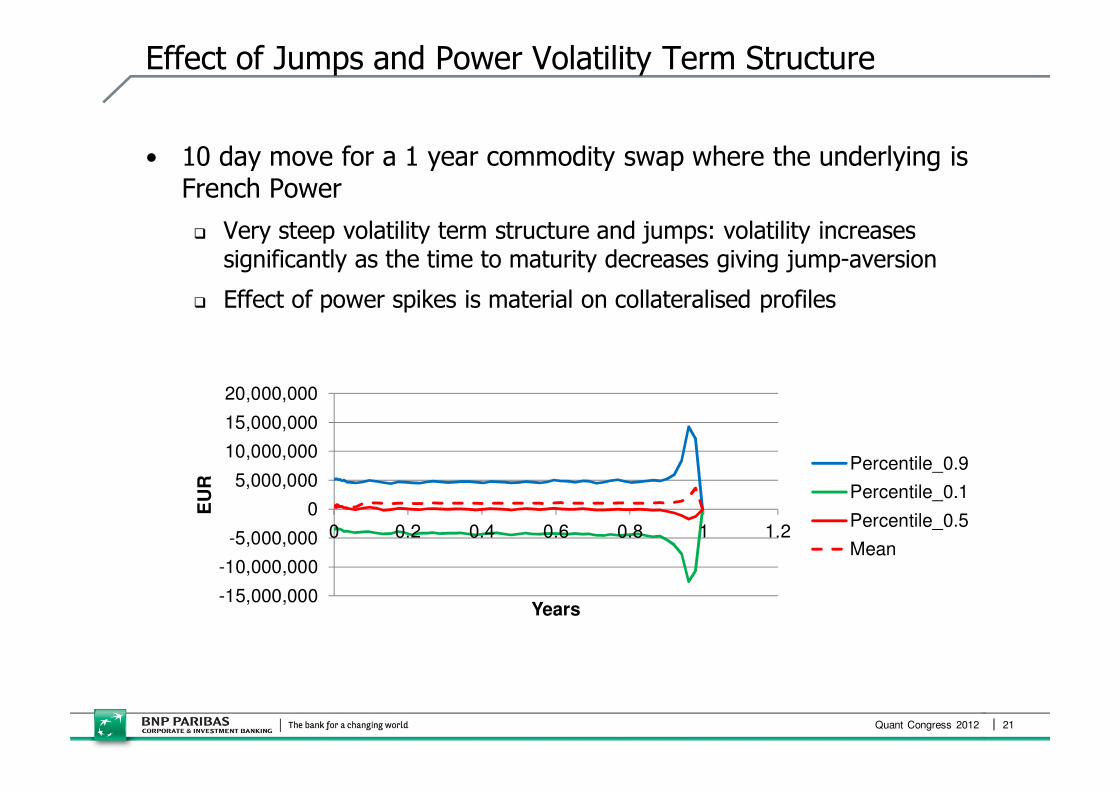
Effect of Jumps and Power Volatility Term Structure

• 10 day move for a 1 year commodity swap where the underlying is French Power

� Very steep volatility term structure and jumps: volatility increases significantly as the time to maturity decreases giving jump-aversion

� Effect of power spikes is material on collateralised profiles

-15,000,000

-10,000,000

-5,000,000

0

5,000,000

10,000,000

15,000,000

20,000,000

0 0.2 0.4 0.6 0.8 1 1.2

EU

R

Years

Percentile_0.9

Percentile_0.1

Percentile_0.5

Mean

• Modelling of pairs of commodities which are co-integrated requires separate consideration

� Such pairs are commonly traded as basis swaps, for example for US gas: the Henry Hub versus Houston Shipping Channel spread, or crack spread: WTI Nymex versus Fuel Oil

� The canonical simulation approach: model all commodities with the 2-factor model used for primaries

� But this does not work well as the distribution of spreads does not reach stationarityin the long-term

• An alternative is to make one of the factors common between the primary and secondary commodity, but this also fails to capture the correct dynamics

• Instead, we model the spread explicitly using a mean-reverting process

or where appropriate the log-normal mean-reverting process. So we have


Model Choice – ‘Secondary’ Commodities

• As illustration, below shows the distribution of the Crude Oil – Fuel Oil crack spread simulated using two approaches: (1) as two primaries, and (2) explicitly as spread:

• Using the primary model, the simulated distributions of Crude Oil and Fuel Oil both show mean-reversion in line with historical data, but the distribution of simulated spread does not

• The distribution of spreads simulated using the secondary model however, reverts in line with historical observations

� Modelling the basis using primaries would lead to much higher PFE for swaps, overcharging capital and CVA


Model Choice – ‘Secondary’ Commodities

-50

0

50

100

150

200

250

300

0 1 2 3 4

Sp

read

[$/M

T]

Simulation Time [years]

envelope usingprimaries model

envelope usingspread model

90th/10th percentile envelopes for simulated

Crude – Fuel Oil spread using two approaches:

the black line is generated using a mean-

reverting spread model whereas the red line is

using two primaries.

:

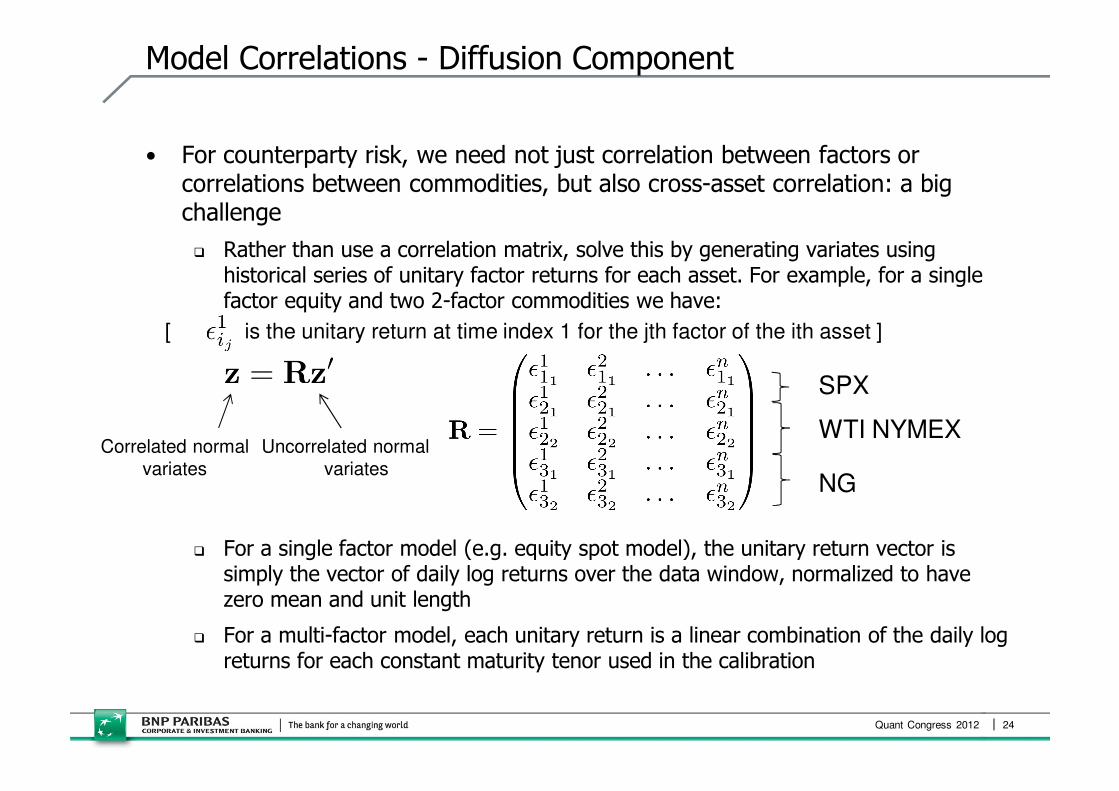
Model Correlations - Diffusion Component

• For counterparty risk, we need not just correlation between factors or correlations between commodities, but also cross-asset correlation: a big challenge

� Rather than use a correlation matrix, solve this by generating variates using historical series of unitary factor returns for each asset. For example, for a single factor equity and two 2-factor commodities we have:

[ is the unitary return at time index 1 for the jth factor of the ith asset ]

� For a single factor model (e.g. equity spot model), the unitary return vector is simply the vector of daily log returns over the data window, normalized to have zero mean and unit length

� For a multi-factor model, each unitary return is a linear combination of the daily log returns for each constant maturity tenor used in the calibration


SPX

WTI NYMEX

NG

Uncorrelated normal

variates

Correlated normal

variates

Model Calibration - Diffusion and Jump Components

• For diffusion component, fit to the covariance matrix of the historical daily log returns for a list of constant maturity tenors

� For example: 1D, 1M, 3M, 6M, 12M, 24M, 36M, 48M, 60M, giving 9x9 covariance matrix

• The fit is to each commodity individually

� This does not explicitly consider cross-underlying elements (e.g. 1M NG to 3M WTI NYMEX)

� This preserves the good scaling properties of the method: computation complexity scales linearly with number of commodities but still gives reasonable correlations cross-underlying / asset


Model Calibration - Diffusion and Jump Components

• A weighted fit of the covariance matrix can be performed

� This gives the ability to:

� Weight less strongly the tenors where the underlying historical data is bad.

� Apply weight to the volatility term structure (i.e. square root of diagonals) more strongly than correlation between different tenors of (invaluable, again, where data is bad)

• Jumps are identified (and removed) from the day-ahead and month-ahead prices:

� A jumps is defined to be a move above 2 standard deviations

• The size and positions of jumps are recorded and concurrent jumps are identified for each commodity group (where jumps occur on the same day) The driving market is identified as the market with the largest (relative) jump


Model Calibration - Diffusion Component

• Process can be summarised as:

1. Fit model parameters (i.e., parameters of volatility functional form, cross-factor correlation) for single underlying, so as to minimize weighted differences of elements of empirical and fitted covariance matrices, in least squares sense. This is a non-linear problem (but not strongly non-linear)

2. Obtain linear combination of tenors that satisfies the fitted parameters above (underdetermined problem) and thence unitary factor returns


1 3 6 12 24 36 60

1 100.0% 98.4% 96.5% 93.4% 87.6% 82.5% 73.4%

3 98.4% 100.0% 99.5% 97.4% 92.6% 87.5% 78.6%

6 96.5% 99.5% 100.0% 99.0% 95.2% 90.6% 82.1%

12 93.4% 97.4% 99.0% 100.0% 98.2% 94.7% 86.8%

24 87.6% 92.6% 95.2% 98.2% 100.0% 98.8% 93.1%

36 82.5% 87.5% 90.6% 94.7% 98.8% 100.0% 97.2%

60 73.4% 78.6% 82.1% 86.8% 93.1% 97.2% 100.0%

1 3 6 12 24 36 60

1 0.0% -1.5% -2.8% -3.6% -2.4% -1.3% -4.3%

3 -1.5% 0.0% -0.2% -0.5% 0.7% 1.4% -1.0%

6 -2.7% -0.2% 0.0% -0.1% 0.8% 1.1% -1.7%

12 -3.4% -0.5% -0.1% 0.0% 0.3% 0.1% -3.4%

24 -2.1% 0.7% 0.8% 0.3% 0.0% -0.4% -4.0%

36 -1.0% 1.4% 1.1% 0.1% -0.4% 0.0% -2.1%

60 -3.2% -1.0% -1.7% -3.4% -4.0% -2.1% 0.0%

0.15

0.2

0.25

0.3

0.35

0.4

0 10 20 30 40 50 60 70

Vo

latility

Tenor in months

Empirical

Fitted

Empirical correlation matrix

Difference between empirical and fitted correlation matrices


Conclusions

• For purposes of computing counterparty risk, a multi-factor model for forward prices is recommended

• Jumps and spikes observed in certain energy commodities prices can affect materially both uncollateralised and collateralised PFE profiles, less for regulatory capital or CVA

• Co-dependence of jumps can be introduced in modelling through a systemic jump process

• Modelling of basis such as crack spreads or US gas pipelines is better captured using a dedicated mean-reverting process

• The three components of the model (primary, secondary and jumps) are well suited to calibrating in the real world measure


References

• L. Clewlow and S. Strickland (1999): A Multi-Factor Model for Energy Derivatives

• R. Gibson & E. Schwartz (1990): Stochastic Convenience Yield and the Pricing of Oil Contingent Claims

• E. Schwartz (1997): The Stochastic Behaviour of Commodity Prices: Implications for Valuation and Hedging

• J. Crosby (2006): A Multi-factor Jump-Diffusion Model for Commodities

• V. Kotecha, V. Chorniy & J. Moorhouse (2012; forthcoming): Modelling Commodities for Counterparty Risk Calculations

Acknowledgement:

We are grateful to Joseph Moorhouse for contributions to this work.

Disclosure:

The views expressed by authors in this presentation are their own and do not necessarily reflect the views of BNP Paribas.


This presentation is for information and illustration purposes only. It does not, nor is it intended to, constitute an offer to acquire, or solicit an offer to acquire any securities or other financial instruments.

This document does not constitute a prospectus and is not intended to provide the sole basis for any evaluation of any

transaction, securities or other financial instruments mentioned herein. To the extent that any transactions is subsequently entered between the recipient and BNP Paribas, such transaction will be entered into upon such terms as may be agreed by the parties in the relevant documentation. Although the information in this document has been obtained from sources

which BNP Paribas believes to be reliable, BNP Paribas does not represent or warrant its accuracy and such information may be incomplete or condensed.

Any person who receives this document agrees that the merits or suitability of any transaction, security or other financial

instrument to such person’s particular situation will have to be independently determined by such person, including consideration of the legal, tax, accounting, regulatory, financial and other related aspects thereof. In particular, BNP Paribas

owes no duty to any person who receives this document (except as required by law or regulation) to exercise any judgement on such person’s behalf as to the merits or suitability of any such transaction, security or other financial instruments. All estimates and opinions included in this document may be subject to change without notice. BNP Paribas

will not be responsible for the consequences of reliance upon any opinion or statement contained herein or for any omission.

This information is not tailored for any particular investor and does not constitute individual investment advice. This document is confidential and is being submitted to selected recipients only. It may not be reproduced (in whole or in part) or delivered to any other person without the prior written permission of BNP Paribas.

© BNP Paribas. All rights reserved. BNP Paribas London Branch (registered office: 10 Harewood Avenue, London NW1 6AA; tel: [44 20] 7595 2000; fax: [44 20] 7595 2555) is authorised and supervised by the Autorité de Contrôle Prudentieland is authorised and subject to limited regulation by the Financial Services Authority. Details of the extent of our

authorisation and regulation by the Financial Services Authority are available from us on request. BNP Paribas London Branch is registered in England and Wales under no. FC13447. www.bnpparibas.com

Disclaimer

modelling commodities for counterparty risk...

Documents