modelling and simulation of standalone solar power … · modelling and simulation of standalone...

A. M. Dizqah, et al., Int. J. Comp. Meth. and Exp. Meas., Vol. 2, No. 1 (2014) 107–125

© 2014 WIT Press, www.witpress.comISSN: 2046-0546 (paper format), ISSN: 2046-0554 (online), http://journals.witpress.comDOI: 10.2495/CMEM-V2-N1-107-125

MODELLING AND SIMULATION OF STANDALONE SOLAR POWER SYSTEMS

A. M. DIZQAH, A. MAHERI, K. BUSAWON & A. KAMJOOFaculty of Engineering and Environment, Northumbria University, Newcastle, UK.

ABSTRACTIn the design of the controllers of hybrid renewable energy system (HRES), the system dynamics and constraints need to be modelled and simulated in conjunction with the controller itself. This paper presents mathematical and equivalent electrical models taking into consideration all system dynamics and constraints for the solar branch of HRES. This branch consists of photovoltaic (PV) array, load and battery connected through a boost-type DC–DC converter. The probabilistic behaviour of the solar irradiance, which intrinsically includes the effect of cloud shading, and the dynamics of the battery are also modelled. The platform developed for dynamic simulation of the solar branch of HRES can be employed for design of DC–DC converter controllers as well as design of energy management systems.Keywords: Battery, boost-type DC–DC converter, electrical load, energy management system, HRES, hybrid renewable energy system, photovoltaic, PV.

1 INTRODUCTIONA system including photovoltaic (PV), converter and battery cannot be modelled with a sys-tem of ordinary differential equations (ODEs). Due to considerable algebraic constraints, the system can only be modelled with a system of differential algebraic equations (DAEs). Moreover, in spite of using some indirect techniques, the current versions of available simulators are not able to solve systems with DAEs directly and this is one of the major challenges in simulating hybrid renewable energy system (HRES).

In order to design controllers and converters for a HRES, it is necessary to model the entire of the system. Altas and Sharaf [1] proposed a simplifi ed model for PV array in Simulink and employed it for simulation of the PV at a specifi c operating point powering constant alternating current and direct current (DC) loads. They used the linearization technique intro-duced by Buresch [2] to take into account the effect of solar irradiation on cell temperature. Villalva et al. [3] proposed two simulation scenarios, both based on equivalent electrical circuits, to simulate a PV module. They also proposed an algorithm for PV identifi cation to fi nd the parameters of equivalent electrical circuit of the PV module. The introduced param-eter identifi cation algorithm by Villalva is based on minimization of the norm of the difference between the calculated power at maximum power point (MPP) and the value provided by the manufacturer. Ishaque et al. [4] introduced a two-diode model for a PV array aiming at increasing the accuracy of the model at low solar radiation. However, their model does not take into account the thermodynamics of the PV panel and its effect on the cell temperature.

Guasch and Silvestre [5] proposed a comprehensive model for lead-acid batteries and an equivalent electrical circuit for simulations.

This paper proposes a comprehensive model of the solar branch of HRES considering the dynamics and constraints that arise due to connecting the components together. A platform for simulation of the solar branch of HRES for the entire of one day is also presented. The developed simulator extracts the required parameters for solar irradiance and PV module modelling from meteorological data and the module datasheet, respectively.

108 A. M. Dizqah, et al., Int. J. Comp. Meth. and Exp. Meas., Vol. 2, No. 1 (2014)

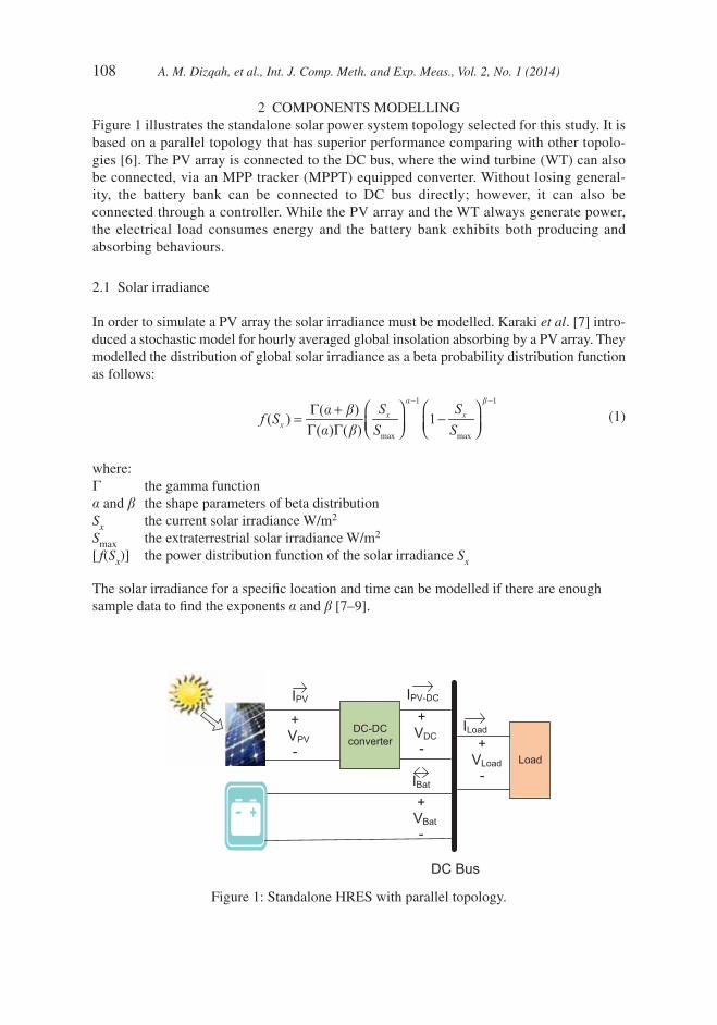
2 COMPONENTS MODELLINGFigure 1 illustrates the standalone solar power system topology selected for this study. It is based on a parallel topology that has superior performance comparing with other topolo-gies [6]. The PV array is connected to the DC bus, where the wind turbine (WT) can also be connected, via an MPP tracker (MPPT) equipped converter. Without losing general-ity, the battery bank can be connected to DC bus directly; however, it can also be connected through a controller. While the PV array and the WT always generate power, the electrical load consumes energy and the battery bank exhibits both producing and absorbing behaviours.

2.1 Solar irradiance

In order to simulate a PV array the solar irradiance must be modelled. Karaki et al. [7] intro-duced a stochastic model for hourly averaged global insolation absorbing by a PV array. They modelled the distribution of global solar irradiance as a beta probability distribution function as follows:

1 1

max max

( )( ) 1( ) ( )

x xx

S Sf S

S S

a b

a b

a b

− −⎛ ⎞ ⎛ ⎞Γ +

= −⎜ ⎟ ⎜ ⎟Γ Γ ⎝ ⎠ ⎝ ⎠ (1)

where:Γ the gamma functiona and b the shape parameters of beta distributionSx the current solar irradiance W/m2

Smax the extraterrestrial solar irradiance W/m2

[ f(Sx)] the power distribution function of the solar irradiance Sx

The solar irradiance for a specifi c location and time can be modelled if there are enough sample data to fi nd the exponents a and b [7–9].

Figure 1: Standalone HRES with parallel topology.

Load

DC Bus

IPV

-

+VPV

IPV-DC

-

+VDC

-

+VBat

IBat

ILoad

-

+VLoad

DC-DC converter

A. M. Dizqah, et al., Int. J. Comp. Meth. and Exp. Meas., Vol. 2, No. 1 (2014) 109

2.2 PV module and PV array

A PV cell is a P–N junction that can be modelled as an electrical circuit [10]. Normally, manufacturers produce PV modules consisting of several PV cells in series. In practice, a PV array which is a combination of several photovoltaic modules in series and parallel arrangement is used to provide appropriate power for a site. A PV panel is a mechanical framework encompasses the PV array. The structure of PV panel and the construction materials infl uence the performance of PV array due to the thermodynamics effects.

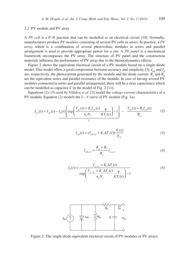
Figure 2 shows the equivalent electrical circuit of a PV module based on a single-diode model. This model offers a good compromise between accuracy and simplicity [3]. Iph and Id are, respectively, the photocurrent generated by the module and the diode current. Rs and Rp are the equivalent series and parallel resistance of the module. In case of having several PV modules connected in series and parallel arrangement, there will be a stray capacitance which can be modelled as capacitor C in the model of Fig. 2 [11].

Equations (2)–(5) used by Villalva et al. [3] model the voltage-current characteristics of a PV module. Equation (2) models the I – V curve of PV module (Fig. 3a).

(2)

,

( )( ) ( ( )) x

ph ph stc i cstc

S tI t I K T t

S= + Δ (3)

, ,

p sph stc sc stc

p

R RI I

R+

= (4)

,0

,

( )( )

( )exp 1

( )

sc stc i c

oc stc v c

d s c

I K T tI t

V K T t qn N KT t

+ Δ=

+ Δ⎛ ⎞−⎜ ⎟⎝ ⎠

(5)

Figure 2: The single-diode equivalent electrical circuit of PV modules or PV arrays.


where VPV and IPV are, respectively, the voltage and current of the PV module and all other symbols are defi ned as follows:

q The electron charge (1.602 × 10−19C)nd Diode ideally factor (−)K The Boltzmann constant (1.38 × 10−23 J/K)Io Reverse saturation current of diode at cell temperature Tx (A)Id The diode current (A)Iph,stc Photocurrent at STC (A)Iph Photocurrent at cell temperature Tx and solar irradiance Sx (A)Isc,stc Short circuit current of PV at STC (A)Voc,stc Open circuit voltage of PV at STC (V)Ns Number of PV cells in series to build PV module (−)Rs Series resistor of array (Ω)Rp Parallel resistor of array (Ω)Ki The factor of the slope of the change in photocurrent due to a change in the cell

temperature (−)Kv The slope of the change in PV voltage due to a change in the solar irradiance (−)Sstc The solar irradiance at STC W/m2

Sx Current amount of solar irradiance W/m2

Tc Current amount of cell temperature (K)ΔTc The difference between current cell temperature and cell temperature at STC (K)

The strictly controlled test conditions (STCs) are a series of metrics in which the performance of PV modules are measured. These test conditions are as follows:

• Cell temperature of 25°C

• Global solar irradiance of 1000 W/m2

• Air Mass of 1.5

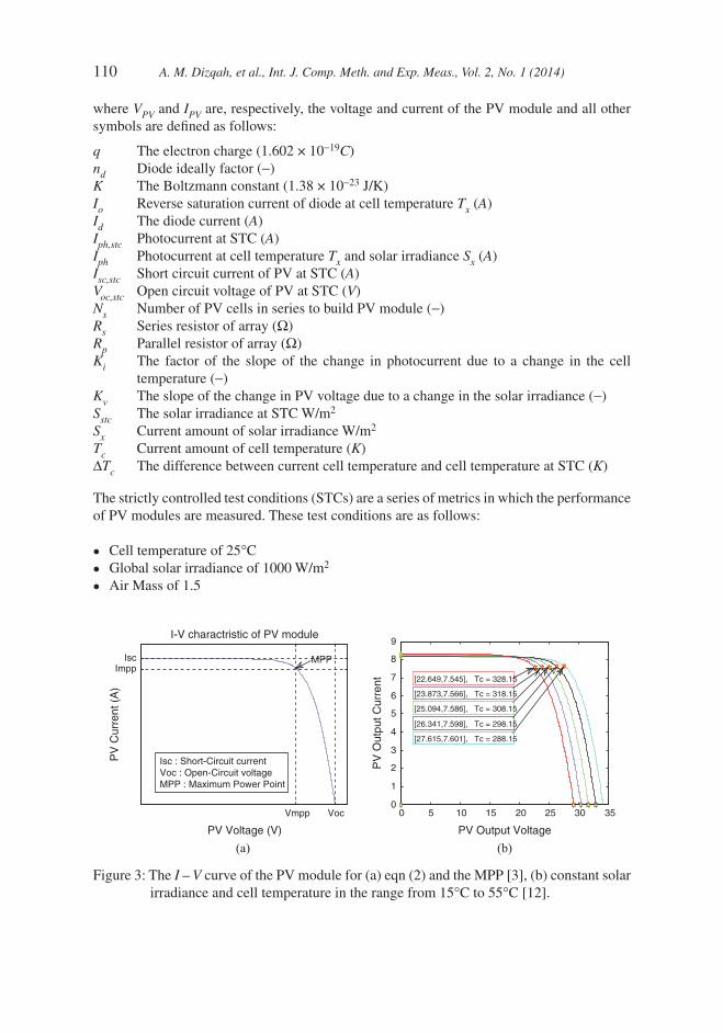
Figure 3: The I – V curve of the PV module for (a) eqn (2) and the MPP [3], (b) constant solar irradiance and cell temperature in the range from 15°C to 55°C [12].

VocVmpp

IscImpp

PV Voltage (V)

PV

Cur

rent

(A

)

I-V charactristic of PV module

Isc : Short-Circuit currentVoc : Open-Circuit voltageMPP : Maximum Power Point

MPP

0 5 10 15 20 25 30 350

1

2

3

4

5

6

7

8

9

PV Output Voltage

PV

Out

put C

urre

nt [22.649,7.545], Tc = 328.15

[25.094,7.586], Tc = 308.15

[26.341,7.598], Tc = 298.15

[27.615,7.601], Tc = 288.15

[23.873,7.566], Tc = 318.15

(a) (b)


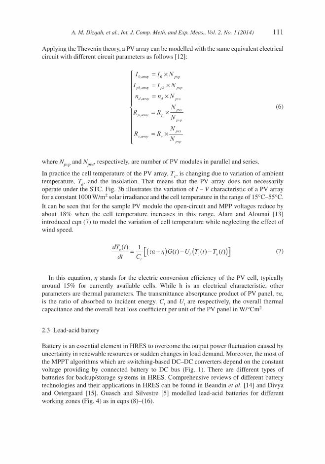
Applying the Thevenin theory, a PV array can be modelled with the same equivalent electrical circuit with different circuit parameters as follows [12]:

0, 0

,

,

,

,

array pvp

ph array ph pvp

d array d pvs

pvsp array p

pvp

pvss array s

pvp

I I N

I I N

n n N

NR R

N

NR R

N

= ×⎧⎪ = ×⎪⎪ = ×⎪⎪⎨

= ×⎪⎪⎪⎪ = ×⎪⎩

(6)

where Npvp and Npvs, respectively, are number of PV modules in parallel and series.

In practice the cell temperature of the PV array, Tc, is changing due to variation of ambient temperature, Ta, and the insolation. That means that the PV array does not necessarily operate under the STC. Fig. 3b illustrates the variation of I – V characteristic of a PV array for a constant 1000 W/m2 solar irradiance and the cell temperature in the range of 15°C–55°C.

It can be seen that for the sample PV module the open-circuit and MPP voltages reduce by about 18% when the cell temperature increases in this range. Alam and Alounai [13] introduced eqn (7) to model the variation of cell temperature while neglecting the effect of wind speed.

( ) ( )( ) 1 ( ) ( ) ( )c

l c at

dT tG t U T t T t

dt Cta h⎡ ⎤= − − −⎣ ⎦ (7)

In this equation, h stands for the electric conversion effi ciency of the PV cell, typically around 15% for currently available cells. While h is an electrical characteristic, other parameters are thermal parameters. The transmittance absorptance product of PV panel, ta, is the ratio of absorbed to incident energy. Ct and Ut are respectively, the overall thermal capacitance and the overall heat loss coeffi cient per unit of the PV panel in W/°Cm2

2.3 Lead-acid battery

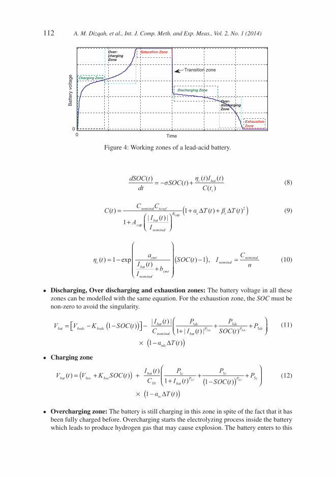
Battery is an essential element in HRES to overcome the output power fl uctuation caused by uncertainty in renewable resources or sudden changes in load demand. Moreover, the most of the MPPT algorithms which are switching-based DC–DC converters depend on the constant voltage providing by connected battery to DC bus (Fig. 1). There are different types of batteries for backup/storage systems in HRES. Comprehensive reviews of different battery technologies and their applications in HRES can be found in Beaudin et al. [14] and Divya and Ostergaard [15]. Guasch and Silvestre [5] modelled lead-acid batteries for different working zones (Fig. 4) as in eqns (8)–(16).


( ) ( )( ) ( )( )

c bat

i

t I tdSOC t SOC tdt C t

hs= − + (8)

( )a b= + Δ + Δ⎛ ⎞

+ ⎜ ⎟⎝ ⎠

2( ) 1 ( ) ( )| ( ) |

1cap

nominal tcoefc cB

batcap

nominal

C CC t T t T t

I tA

I

(9)

( )( ) 1 exp ( ) 1 , ( )cmt nominal

c nominalbat

cmtnominal

a Ct SOC t I

I t nbI

h

⎛ ⎞⎜ ⎟

= − − =⎜ ⎟⎜ ⎟+⎜ ⎟⎝ ⎠

(10)

• Discharging, Over discharging and exhaustion zones: The battery voltage in all these zones can be modelled with the same equation. For the exhaustion zone, the SOC must be non-zero to avoid the singularity.

(11)

• Charging zone

( )( )

( )a

⎛ ⎞= + + + +⎜ ⎟+ −⎝ ⎠

× − Δ

2 4

1 35

10

( )( ) ( )

1 ( ) 1 ( )

1 ( )

C C

bat c cbat boc boc cP P

bat

rc

I t P PV t V K SOC t P

C I t SOC t

T t

(12)

• Overcharging zone: The battery is still charging in this zone in spite of the fact that it has been fully charged before. Overcharging starts the electrolyzing process inside the battery which leads to produce hydrogen gas that may cause explosion. The battery enters to this

Figure 4: Working zones of a lead-acid battery.

00

Time

Bat

tery

vol

tage Charging Zone

ExhaustionZone

Discharging Zone

Over-dischargingZone

Saturation ZoneOver-chargingZone

Transition zone


zone when Vbat ≥ Vg, where Vg is the gassing voltage of the battery and the voltage of the battery increases up to the saturation voltage (Vec).

( ) ( ) ( ) ( )( ) ( ) ( ( ) ( )) 1 exp

( ) ( )

g

nominalV

nbat g ec g

bat

CSOC t C t SOC t C t

CV t V t V t V t

I t tt

⎡ ⎤⎛ ⎞−⎢ ⎥⎜ ⎟⎢ ⎥= + − × − ⎜ ⎟⎢ ⎥⎜ ⎟⎢ ⎥⎜ ⎟⎝ ⎠⎣ ⎦

(13)

( )( )

( ) ln 1 1 ( )batg gas gas gas

nominal

I tV t A B T t

Ca

⎡ ⎤⎛ ⎞= + + − Δ⎢ ⎥⎜ ⎟⎝ ⎠⎢ ⎥⎣ ⎦

(14)

( )( )

( ) ln 1 1 ( )batec fonsc fonsc fc

nominal

I tV t A B T t

Ca

⎡ ⎤⎛ ⎞= + + − Δ⎢ ⎥⎜ ⎟⎝ ⎠⎢ ⎥⎣ ⎦

(15)

( )( )( )

1 scbat

nominal

SCCI t

sc C

At

B t

t

t

t =+

(16)

where:Cnominal The rated battery capacity at nominal discharging current (h)Inominal The nominal discharge current corresponding to Cnominal (A)DT The temperature variation from the reference value of 25°C (K)n The time (h)ac The temperature coeffi cient (K−1)bc The temperature coeffi cient (K−2)Ctcoeff ,Acap,Bcap ,acmt ,bcmt The model constants (−)hc The charging effi ciency (−)I10 The nominal discharge current for the period of 10 hours (A)

P2dc ,P2c ,P5dc ,P5c The model constants (Vh)

P1dc ,P1c The model constants (VAh)

P2dc ,P2c ,P4dc ,P4c ,Ctsc The model constants (−)

Pbodc ,Kboc ,Vbodc ,Vboc

Agas ,Bgas ,Afonc ,Bfonc The model constants (V)

ardc , arc , agas , afc The temperature coeffi cient (K−1)t The time factor (−)Atsc , Btsc The model constants (h)Vg The nominal gassing voltage of the battery (V)Vec The saturation voltage of the battery (V)SOCVg The SOC of the battery at the gassing voltage (−)SOC The battery state of charge (–)Ibat The battery current (A)Vbat The battery voltage (V)s The self-discharge rate (0.2% per day)C The battery instantaneous capacity (Ah)C10 The battery 10-hour rated capacity (Ah)


2.4 Boost-type DC–DC converter

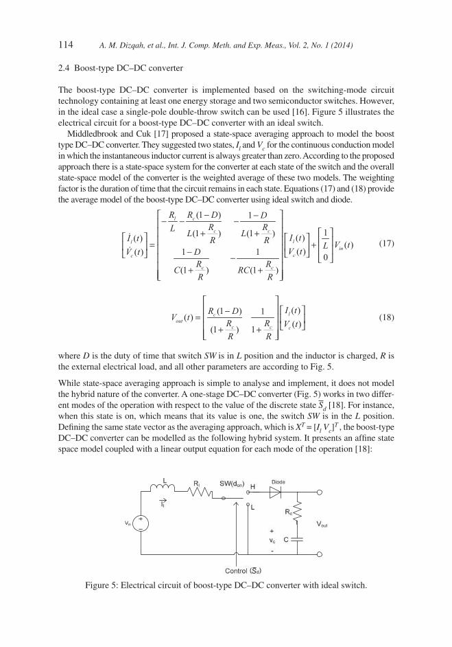
The boost-type DC–DC converter is implemented based on the switching-mode circuit technology containing at least one energy storage and two semiconductor switches. However, in the ideal case a single-pole double-throw switch can be used [16]. Figure 5 illustrates the electrical circuit for a boost-type DC–DC converter with an ideal switch.

Middledbrook and Cuk [17] proposed a state-space averaging approach to model the boost type DC–DC converter. They suggested two states, Il and Vc for the continuous conduction model in which the instantaneous inductor current is always greater than zero. According to the proposed approach there is a state-space system for the converter at each state of the switch and the overall state-space model of the converter is the weighted average of these two models. The weighting factor is the duration of time that the circuit remains in each state. Equations (17) and (18) provide the average model of the boost-type DC–DC converter using ideal switch and diode.

(1 ) 1

1(1 ) (1 ) ( )( )( )

( )( ) 1 1 0(1 ) (1 )

l c

c c

llin

cc

c c

R R D DR RL L L I tI t R R V tLV tV t D

R RC RC

R R

− −⎡ ⎤− − −⎢ ⎥⎢ ⎥ ⎡ ⎤+ +⎡ ⎤ ⎡ ⎤⎢ ⎥ ⎢ ⎥= +⎢ ⎥ ⎢ ⎥⎢ ⎥ ⎢ ⎥− ⎣ ⎦⎣ ⎦ −⎢ ⎥ ⎣ ⎦⎢ ⎥+ +⎢ ⎥⎣ ⎦

&

& (17)

( )(1 ) 1( )( )(1 ) 1

lcout

c c c

I tR DV t

R R V tR R

⎡ ⎤⎢ ⎥ ⎡ ⎤−

= ⎢ ⎥ ⎢ ⎥⎣ ⎦⎢ ⎥+ +⎢ ⎥⎣ ⎦

(18)

where D is the duty of time that switch SW is in L position and the inductor is charged, R is the external electrical load, and all other parameters are according to Fig. 5.

While state-space averaging approach is simple to analyse and implement, it does not model the hybrid nature of the converter. A one-stage DC–DC converter (Fig. 5) works in two differ-ent modes of the operation with respect to the value of the discrete state S d [18]. For instance, when this state is on, which means that its value is one, the switch SW is in the L position. Defi ning the same state vector as the averaging approach, which is XT = [Il Vc]

T , the boost-type DC–DC converter can be modelled as the following hybrid system. It presents an affi ne state space model coupled with a linear output equation for each mode of the operation [18]:

Figure 5: Electrical circuit of boost-type DC–DC converter with ideal switch.

S


1 1

2 2

( ) ( ); 1( )

( ) ( ); 0in d

in d

F X t f V t SX t

F X t f V t S⎧ + =

= ⎨ + =⎩& (19)

1

2

( ); 1( )

( ); 0

Td

out Td

g X t SV t

g X t S⎧ =

= ⎨ =⎩ (20)

1 2 1 2

1

0 11 (1 ), , 1 1 10 0

( )(1 ) (1 )

cl

l c c

c c c

RRR R RL LL R RF F f f L

C R R R RC RC

R R

⎡ ⎤− − −⎢ ⎥⎡ ⎤− ⎢ ⎥ ⎡ ⎤+ +⎢ ⎥⎢ ⎥ ⎢ ⎥⎢ ⎥= = = =⎢ ⎥ ⎢ ⎥⎢ ⎥− −⎢ ⎥ ⎣ ⎦⎢ ⎥+⎣ ⎦ ⎢ ⎥+ +⎢ ⎥⎣ ⎦

(21)

1 21 1 0 ,

1 1 1

T T

c

c c c

Rg g

R R RR R R

⎡ ⎤ ⎡ ⎤⎢ ⎥ ⎢ ⎥

= =⎢ ⎥ ⎢ ⎥⎢ ⎥ ⎢ ⎥+ + +⎢ ⎥ ⎢ ⎥⎣ ⎦ ⎣ ⎦

(22)

2.5 Load profi le

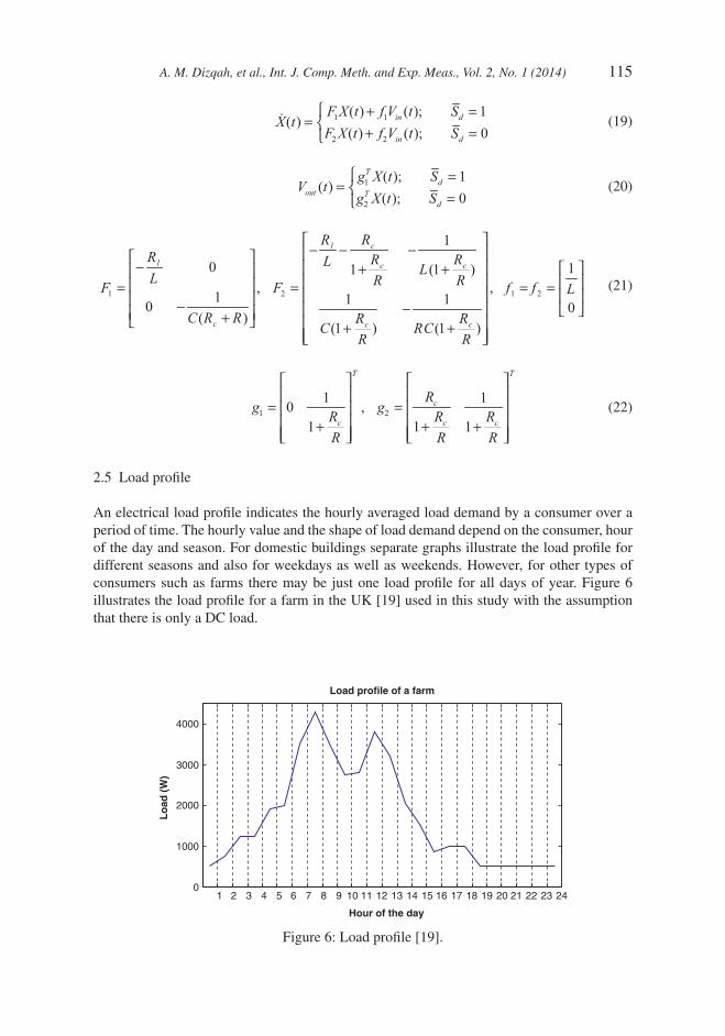
An electrical load profi le indicates the hourly averaged load demand by a consumer over a period of time. The hourly value and the shape of load demand depend on the consumer, hour of the day and season. For domestic buildings separate graphs illustrate the load profi le for different seasons and also for weekdays as well as weekends. However, for other types of consumers such as farms there may be just one load profi le for all days of year. Figure 6 illustrates the load profi le for a farm in the UK [19] used in this study with the assumption that there is only a DC load.

Figure 6: Load profi le [19].

1 2 3 4 5 6 7 8 9 10 11 12 13 14 15 16 17 18 19 20 21 22 23 240

1000

2000

3000

4000

Hour of the day

Lo

ad (

W)

Load profile of a farm


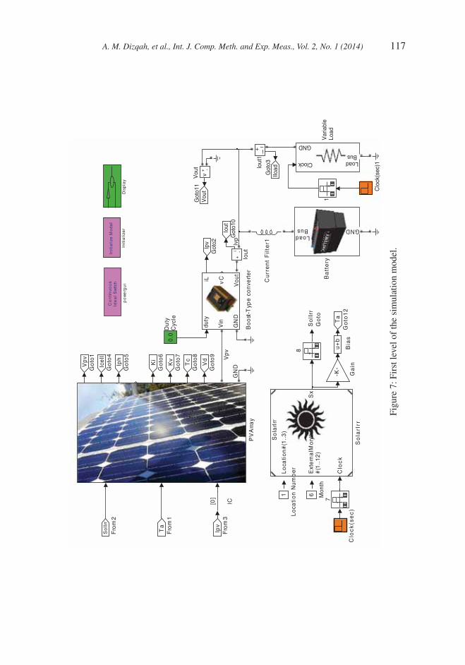
3 SIMULATIONDifferent components of the standalone solar site can be simulated with general blocks and equivalent electrical circuits. The fi rst level of the simulation model is given in Fig. 7. As it can be seen there are fi ve main blocks in this model. While SolarIrr simulates solar irradiance, PVArray simulates an array of PV modules. In addition, the block with the name of Boost-Type Converter provides the simulation of DC–DC converter. Battery and Load blocks, respectively, simulate a stack of lead-acid battery cells and the load profi le.

3.1 Solar irradiance simulation

The simulation proposed in this paper for solar irradiance is based on the hourly stochastic model of eqn (1). Although, there are inaccuracies in fi tting solar irradiance into beta distribution still there are two advantages the simulation can benefi t from stochastic modelling.

The main advantage of stochastic modelling of solar irradiance is its simplicity for simulation. Once the shape parameters are learned for all hours of the year, the value of insolation can be generated easily by using random generators. Another advantage of generating random values for solar irradiance is that uncertainties due to cloud shading or incident angle are intrinsically taken into account and the generated values of the solar irradiance are directly fed into the PV cell.

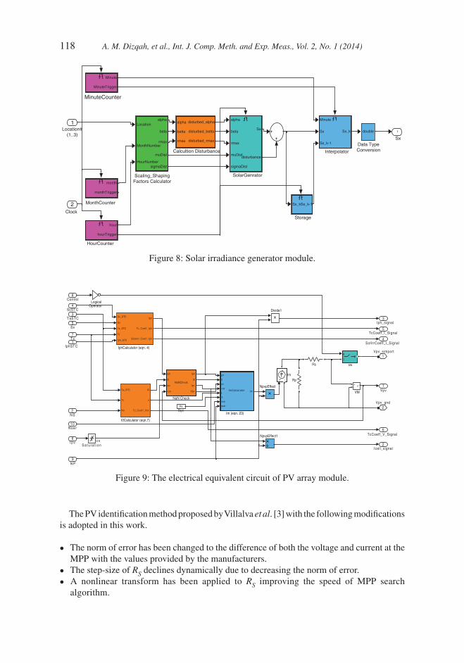
In calculation of the shape parameters for hourly solar irradiance, the meteorological sample data available from British Atmospheric Data Centre [20] between 1990 and 2010 have been used. The calculated shape parameters load into lookup tables and used to generate random values for hourly solar irradiance (Fig. 8).

There are two challenges in simulating the insolation coupled with other components. First, it causes the simulation to be multi-rate. While the time step for all components is small enough to simulate the system dynamics, the simulation rate of the solar irradiance is one hour, which is signifi cantly higher. In this study, this challenge has been overcome by feeding a separate clock to SolarIrr block (Fig. 7). Second, singularity can occur during simulation by hourly stepwise solar irradiance. An interpolator has been employed to solve this problem with linearizing the transition of solar irradiance between hours.

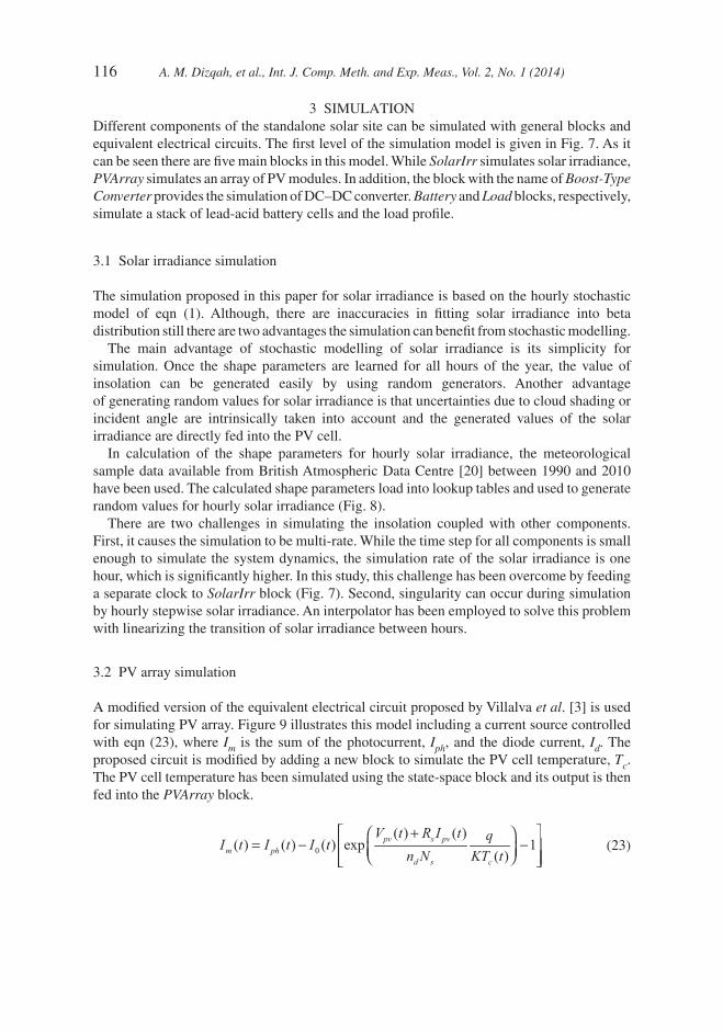
3.2 PV array simulation

A modifi ed version of the equivalent electrical circuit proposed by Villalva et al. [3] is used for simulating PV array. Figure 9 illustrates this model including a current source controlled with eqn (23), where Im is the sum of the photocurrent, Iph, and the diode current, Id. The proposed circuit is modifi ed by adding a new block to simulate the PV cell temperature, Tc. The PV cell temperature has been simulated using the state-space block and its output is then fed into the PVArray block.

0

( ) ( )( ) ( ) ( ) exp 1

( )pv s pv

m phd s c

V t R I t qI t I t I tn N KT t

⎡ ⎤+⎛ ⎞= − −⎢ ⎥⎜ ⎟⎝ ⎠⎢ ⎥⎣ ⎦

(23)


Figu

re 7

: Fir

st le

vel o

f th

e si

mul

atio

n m

odel

.

Co

ntin

uo

us

Ide

al

Sw

itch

po

we

rgu

i

v+ -

Vou

t

Clock

GND

LoadBus

Var

iabl

eLo

ad

So

larI

rr

Lo

cati

on

#(1

..3

)

Ext

ern

alM

on

th#

(1..

12

)

Clo

ck

Sx

So

larI

rr

PV

Arr

ay

6 Mon

th

1

Lo

cati

on

Nu

mb

er

i+ –

Iout

1

i+

-

IoutIn

itia

lize

Mo

de

l

Init

iali

zer

[0]

IC

Vd

Go

to9

Tc

Go

to8

Kv

Go

to7

Ki

Go

to6

Iph

Go

to5

Ice

llG

oto

4

Iload

Got

o3

Ipv

Got

o2

Ta

Go

to1

2

Vou

tG

oto1

1

Iout

Got

o10

Vp

vG

oto

1

So

lIrr

Go

to

-K-

Ga

in

Ipv

Fro

m3

So

lIrr

Fro

m2

Ta

Fro

m1

0.0

Du

tyC

ycle

Dis

pla

y

Cu

rre

nt

Fil

ter1

Clo

ck(s

ec)1

Clo

ck

(se

c)

duty

iL vC

Vin

GN

DV

out

Bo

ost

-Typ

e c

on

vert

er

u+

b

Bia

s

LoadBus GND

Ba

tte

ry

8

71

GN

DIv

p

Vpv


The PV identifi cation method proposed by Villalva et al. [3] with the following modifi cations is adopted in this work.

• The norm of error has been changed to the difference of both the voltage and current at the MPP with the values provided by the manufacturers.

• The step-size of RS declines dynamically due to decreasing the norm of error.

• A nonlinear transform has been applied to RS improving the speed of MPP search algorithm.

Figure 9: The electrical equivalent circuit of PV array module.

6TcCoeff_V_Signal

5TcCoeff_I_Signal

4SolIrrCoeff_I_Signal

3Iph_signal

2Icell_signal

1Vpv

2Vpv_gnd

1Vpv_simport

g

12

sw

v+-

VM

S a t u r a t i o n

Rs

Rs1

Rs

Rp

NpvpEffect1

NpvpEffect

iph

i0

ipv

v pv

Iph

I0

Ipv

Vpv

NaNCheck

NaN Check

LogicalOperator

Sc_STC

Sx

Ta_STC

Tc

Iph_STC

Iph

Tc_Coef f _Iph

SolarIrr_Coef f _Iph

IphCalculator (eqn. 4)

iph

i0

ipv

v pv

a

rs

nser

npar

ImImCalculator

Im (eqn. 23)

s -+

Im

Ta_STC

Tc

Ns

I0

a

Tc_Coef f _Voc

I0Calculator (eqn.7)

Divide1

1 0N s e r

9N P

8Control

7Tc

6I p v

5Sx

4ScSTC

3T aSTC

2N S

1IphST C

u u

Figure 8: Solar irradiance generator module.

1

Sx

Sx_kSx_k-1

Storage

alpha

beta

rmax

muDist

sigmaDist

Sx

disturbance

SolarGenrator

Location

MonthNumber

HourNumber

alpha

beta

rmax

muDist

sigmaDist

Scaling_ShapingFactors Calculatormonth

monthTrigger

MonthCounter

Minute

MinuteTrigger

MinuteCounter

Minute

Sx

Sx_k-1

Sx_k

Interpolator

hour

hourTrigger

HourCounter

double

Data TypeConversion

alpha

betta

rmax

disturbed_alpha

disturbed_betta

disturbed_rmax

Calcultion Disturbance

2Clock

1Location#

(1..3)


Although the PV array as a component can be simulated with its equivalent electrical circuit, there is still a challenge in its connection to DC–DC converter. Since the PV array is an instantaneous system [eqn (2)], its connection to the converter casts an algebraic constraint on the converter which is not solvable with ordinary ODE integrators. It requires employing a DAE integrator to simulate such a system directly. In the present study, however, a combination of an ordinary integrator coupled with a Newton type method, which solves the algebraic constraints, have been employed. It requires using a small step-size for the simulation (i.e. 10−8 sec.) and setting manually a consistent initial value.

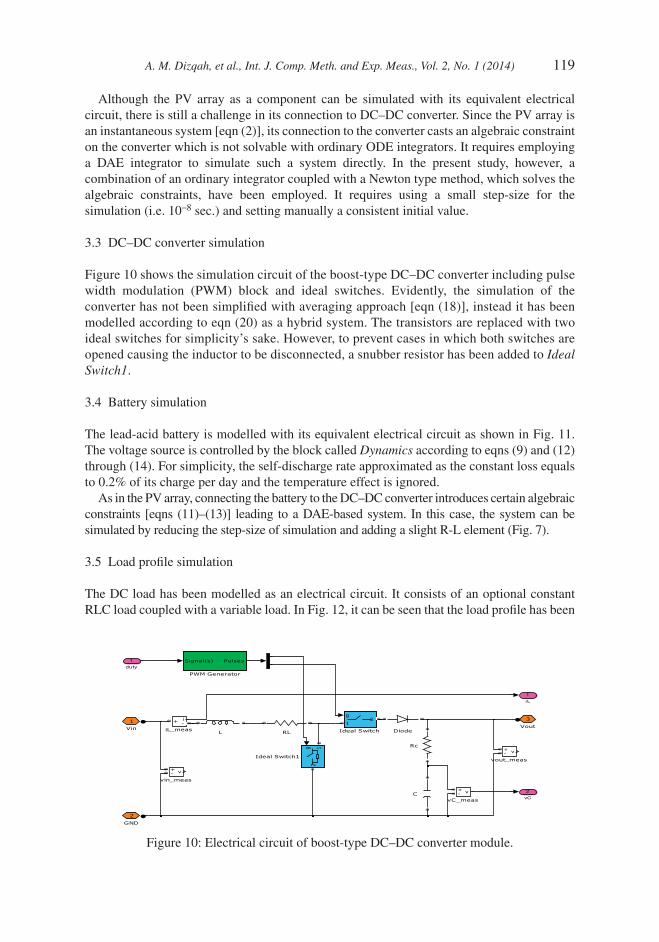
3.3 DC–DC converter simulation

Figure 10 shows the simulation circuit of the boost-type DC–DC converter including pulse width modulation (PWM) block and ideal switches. Evidently, the simulation of the converter has not been simplifi ed with averaging approach [eqn (18)], instead it has been modelled according to eqn (20) as a hybrid system. The transistors are replaced with two ideal switches for simplicity’s sake. However, to prevent cases in which both switches are opened causing the inductor to be disconnected, a snubber resistor has been added to Ideal Switch1.

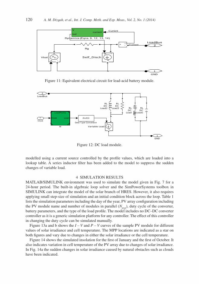
3.4 Battery simulation

The lead-acid battery is modelled with its equivalent electrical circuit as shown in Fig. 11. The voltage source is controlled by the block called Dynamics according to eqns (9) and (12) through (14). For simplicity, the self-discharge rate approximated as the constant loss equals to 0.2% of its charge per day and the temperature effect is ignored.

As in the PV array, connecting the battery to the DC–DC converter introduces certain algebraic constraints [eqns (11)–(13)] leading to a DAE-based system. In this case, the system can be simulated by reducing the step-size of simulation and adding a slight R-L element (Fig. 7).

3.5 Load profi le simulation

The DC load has been modelled as an electrical circuit. It consists of an optional constant RLC load coupled with a variable load. In Fig. 12, it can be seen that the load profi le has been

Figure 10: Electrical circuit of boost-type DC–DC converter module.

2vC

1iL

3

Vout

2

GND

1

Vin

v+-

vout_meas

v+-

vin_meas

v+-

vC_meas

i+ -

iL_meas

Rc

RL

Signal(s) Pulses

PWM Generator

L

g 12

Ideal Switch1

g

12

Ideal Switch Diode

C

1duty


modelled using a current source controlled by the profi le values, which are loaded into a lookup table. A series inductor fi lter has been added to the model to suppress the sudden changes of variable load.

4 SIMULATION RESULTSMATLAB/SIMULINK environment was used to simulate the model given in Fig. 7 for a 24-hour period. The built-in algebraic loop solver and the SimPowerSystems toolbox in SIMULINK can integrate the model of the solar branch of HRES. However, it also requires applying small step-size of simulation and an initial condition block across the loop. Table 1 lists the simulation parameters including the day of the year, PV array confi guration including the PV module name and number of modules in parallel (Npvp), duty cycle of the converter, battery parameters, and the type of the load profi le. The model includes no DC–DC converter controller as it is a generic simulation platform for any controller. The effect of this controller in changing the duty cycle can be simulated manually.

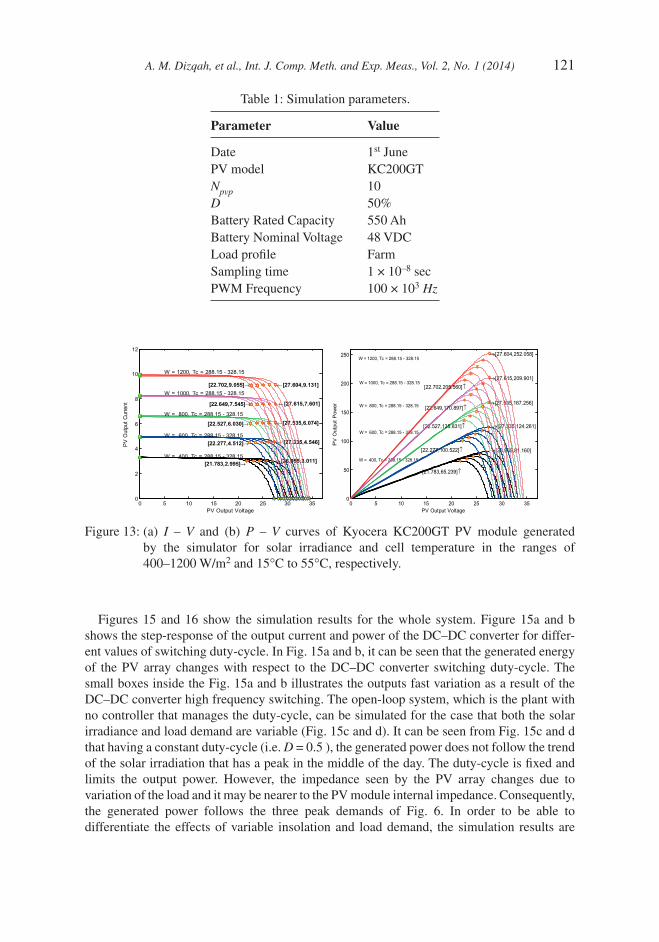
Figure 13a and b shows the I – V and P – V curves of the sample PV module for different values of solar irradiance and cell temperature. The MPP locations are indicated as a star on both fi gures and vary due to changes in either the solar irradiance or the cell temperature.

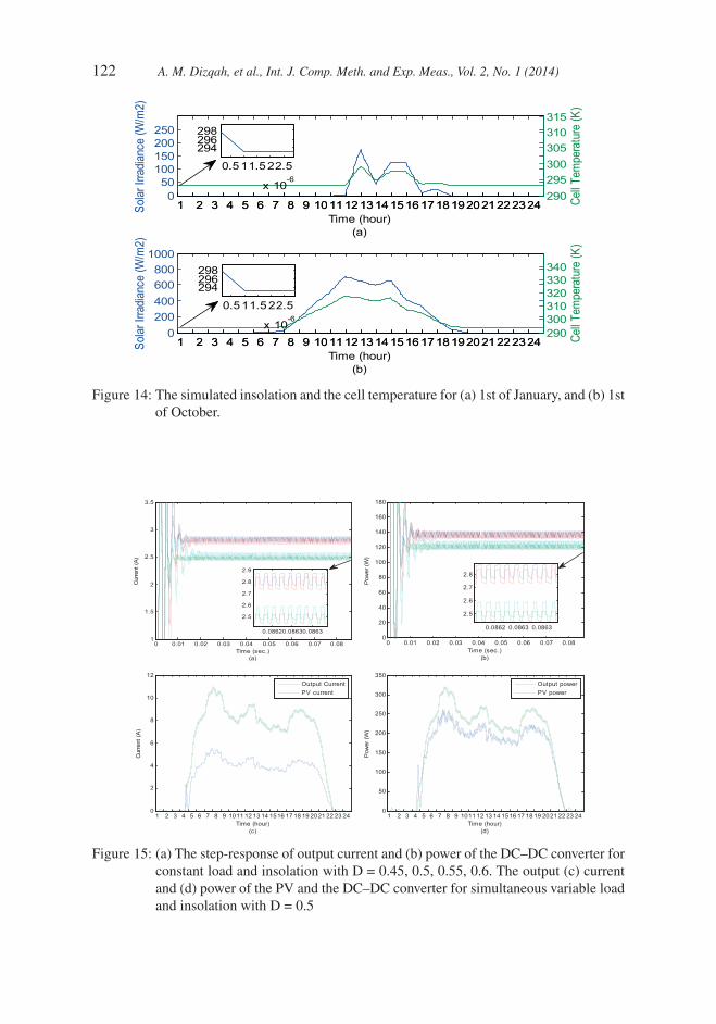
Figure 14 shows the simulated insolation for the fi rst of January and the fi rst of October. It also indicates variation in cell temperature of the PV array due to changes of solar irradiance. In Fig. 14a the sudden changes in solar irradiance caused by natural obstacles such as clouds have been indicated.

Figure 11: Equivalent electrical circuit for lead-acid battery module.

Rg

Vbat

2LoadBus

1

GND

s -+

Self_Disch

currentV

Isd

Dynamics (Eqns. 9, 12, 13, 14)

i+ -

s -+

Current

Current

Figure 12: DC load module.

2LoadBus

1GND

s -+

Variable Load

RLDC

Load3

RLDC

Load2 RLDC

Load1

RLDC

LoadLoadProfile

Clock Load

M

double

Data Type Conversion

1Clock


Table 1: Simulation parameters.

Parameter Value

Date 1st JunePV model KC200GTNpvp 10D 50%Battery Rated Capacity 550 AhBattery Nominal Voltage 48 VDCLoad profi le FarmSampling time 1 × 10–8 secPWM Frequency 100 × 103 Hz

Figure 13: (a) I – V and (b) P – V curves of Kyocera KC200GT PV module generated by the simulator for solar irradiance and cell temperature in the ranges of 400–1200 W/m2 and 15°C to 55°C, respectively.

0 5 10 15 20 25 30 350

2

4

6

8

10

12

¨[26.955,3.011]W = 400, Tc = 288.15 - 328.15

[21.783,2.995]Æ

¨[27.335,4.546]W = 600, Tc = 288.15 - 328.15

[22.277,4.512]Æ

¨[27.535,6.074]W = 800, Tc = 288.15 - 328.15

[22.527,6.030]Æ

¨[27.615,7.601]

W = 1000, Tc = 288.15 - 328.15

[22.649,7.545]Æ

¨[27.604,9.131]

W = 1200, Tc = 288.15 - 328.15

[22.702,9.055]Æ

PV Output Voltage

PV

Out

put C

urre

nt

0 5 10 15 20 25 30 350

50

100

150

200

250

→[26.955,81.160]

W = 400, Tc = 288.15 - 328.15

[21.783,65.239]↑

→[27.335,124.261]W = 600, Tc = 288.15 - 328.15

[22.277,100.522]↑

→[27.535,167.256]W = 800, Tc = 288.15 - 328.15

[22.527,135.831]↑

→[27.615,209.901]W = 1000, Tc = 288.15 - 328.15

[22.649,170.897]↑

→[27.604,252.058]W = 1200, Tc = 288.15 - 328.15

[22.702,205.560]↑

PV Output Voltage

PV

Out

put P

ower

Figures 15 and 16 show the simulation results for the whole system. Figure 15a and b shows the step-response of the output current and power of the DC–DC converter for differ-ent values of switching duty-cycle. In Fig. 15a and b, it can be seen that the generated energy of the PV array changes with respect to the DC–DC converter switching duty-cycle. The small boxes inside the Fig. 15a and b illustrates the outputs fast variation as a result of the DC–DC converter high frequency switching. The open-loop system, which is the plant with no controller that manages the duty-cycle, can be simulated for the case that both the solar irradiance and load demand are variable (Fig. 15c and d). It can be seen from Fig. 15c and d that having a constant duty-cycle (i.e. D = 0.5 ), the generated power does not follow the trend of the solar irradiation that has a peak in the middle of the day. The duty-cycle is fi xed and limits the output power. However, the impedance seen by the PV array changes due to variation of the load and it may be nearer to the PV module internal impedance. Consequently, the generated power follows the three peak demands of Fig. 6. In order to be able to differentiate the effects of variable insolation and load demand, the simulation results are


Figure 14: The simulated insolation and the cell temperature for (a) 1st of January, and (b) 1st of October.

1 2 3 4 5 6 7 8 9 10 11 12 13 14 15 16 17 18 19 20 21 22 23 240

50100150200250

Solar

Irra

dianc

e (W

/m2)

Time (hour)(a)

1 2 3 4 5 6 7 8 9 10 11 12 13 14 15 16 17 18 19 20 21 22 23 24290295300305310315

Cell T

empe

ratu

re (K

)

1 2 3 4 5 6 7 8 9 10 11 12 13 14 15 16 17 18 19 20 21 22 23 240

200400600800

1000

Solar

Irra

dianc

e (W

/m2)

Time (hour)(b)

1 2 3 4 5 6 7 8 9 10 11 12 13 14 15 16 17 18 19 20 21 22 23 24290300310320330340

Cell T

empe

ratu

re (K

)

0.511.522.5

x 10-6

294296298

0.511.522.5

x 10-6

294296298

Figure 15: (a) The step-response of output current and (b) power of the DC–DC converter for constant load and insolation with D = 0.45, 0.5, 0.55, 0.6. The output (c) current and (d) power of the PV and the DC–DC converter for simultaneous variable load and insolation with D = 0.5

0 0.01 0.02 0.03 0.04 0.05 0.06 0.07 0.081

1.5

2

2.5

3

3.5

Cur

rent

(A)

Time (sec.)(a)

0.08620.08630.0863

2.5

2.6

2.7

2.8

2.9

0 0.01 0.02 0.03 0.04 0.05 0.06 0.07 0.080

20

40

60

80

100

120

140

160

180

Pow

er (W

)

Time (sec.)(b)

0.0862 0.0863 0.0863

2.5

2.6

2.7

2.8

1 2 3 4 5 6 7 8 9 10 11 12 13 14 15 16 17 18 19 20 21 22 23 240

2

4

6

8

10

12

Cur

rent

(A)

Time (hour)(c)

Output CurrentPV current

1 2 3 4 5 6 7 8 9 10 11 12 13 14 15 16 17 18 19 20 21 22 23 240

50

100

150

200

250

300

350

Pow

er (W

)

Time (hour)(d)

Output powerPV power


organized into two separate cases: (i) a constant load coupled with varying insolation, and (ii) a constant insolation with variable load.

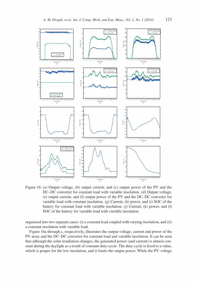
Figure 16a through c, respectively, illustrates the output voltage, current and power of the PV array and the DC–DC converter for constant load and variable insolation. It can be seen that although the solar irradiation changes, the generated power (and current) is almost con-stant during the daylight as a result of constant duty-cycle. The duty-cycle is fi xed to a value, which is proper for the low insolation, and it limits the output power. While the PV voltage

Figure 16: (a) Output voltage, (b) output current, and (c) output power of the PV and the DC–DC converter for constant load with variable insolation. (d) Output voltage, (e) output current, and (f) output power of the PV and the DC–DC converter for variable load with constant insolation. (g) Current, (h) power, and (i) SOC of the battery for constant load with variable insolation. (j) Current, (k) power, and (l) SOC of the battery for variable load with variable insolation.

1 2 3 4 5 6 7 8 9 10 11 12 13 14 15 16 17 18 19 20 21 22 23 240

5

10

15

20

25

30

35

40

45

50

55

Vol

tage

(V)

Time (hour)(a)

Output voltagePV voltage

1 2 3 4 5 6 7 8 9 10 11 12 13 14 15 16 17 18 19 20 21 22 23 240

2

4

6

8

10

12

Cur

rent

(A)

Time (hour)(b)


1 2 3 4 5 6 7 8 9 10 11 12 13 14 15 16 17 18 19 20 21 22 23 240

50

100

150

200

250

300

350

Pow

er (W

)

Time (hour)(c)


1 2 3 4 5 6 7 8 9 10 11 12 13 14 15 16 17 18 19 20 21 22 23 240

5

10

15

20

25

30

35

40

45

50

55

Vol

tage

(V)

Time (hour)(d)

Output voltagePV voltage

1 2 3 4 5 6 7 8 9 10 11 12 13 14 15 16 17 18 19 20 21 22 23 240

2

4

6

8

10

12

Cur

rent

(A)

Time (hour)(e)


1 2 3 4 5 6 7 8 9 10 11 12 13 14 15 16 17 18 19 20 21 22 23 240

50

100

150

200

250

300

350

Pow

er (W

)

Time (hour)(f)


1 2 3 4 5 6 7 8 9 10 11 12 13 14 15 16 17 18 19 20 21 22 23 24-2

-1

0

1

2

3

4

5

Cur

rent

(A)

Time (hour)(g)

1 2 3 4 5 6 7 8 9 10 11 12 13 14 15 16 17 18 19 20 21 22 23 24-100

-50

0

50

100

150

200

250

Pow

er (W

)

Time (hour)(h)

1 2 3 4 5 6 7 8 9 10 11 12 13 14 15 16 17 18 19 20 21 22 23 2476

76.5

77

77.5

78

78.5

79

79.5

80

80.5

81

SO

C (%

)

Time (hour)(i)

1 2 3 4 5 6 7 8 9 10 11 12 13 14 15 16 17 18 19 20 21 22 23 24

0

5

10

15

20

25

30

Cur

rent

(A)

Time (hour)(j)

Battery CurrentLoad Current

1 2 3 4 5 6 7 8 9 10 11 12 13 14 15 16 17 18 19 20 21 22 23 24-100

0

100

200

300

400

500

600

700

800

Pow

er (W

)

Time (hour)(k)

1 2 3 4 5 6 7 8 9 10 11 12 13 14 15 16 17 18 19 20 21 22 23 2450

55

60

65

70

75

80

SO

C (%

)

Time (hour)(l)


changes during the day, the output voltage of the DC–DC converter, which is connected directly to the battery terminal, is almost constant (Fig. 16a). Moreover, there is around 20% difference between the PV and the DC–DC output powers which is a power loss due to the internal resistor of the solenoid, Rl (Fig. 5). It is assumed that there is excess of energy dur-ing the daylight that is stored into the connected battery. Figure 16g through l shows the current, power, and the state of charge (SOC) of the battery. The direction of the battery current in Fig. 16g shows that the battery is charged and the battery SOC increases during the daylight.

On the other hand, Fig. 16d through f, respectively, depicts the system variables for the constant insolation and variable load. Although the solar irradiation is constant, any load demand fl uctuation leads to the change in the input impedance seen by the PV module (Fig. 1) when the duty-cycle is constant. Therefore, the generated power by the PV array slightly changes. Figure 16g through l shows the current, power, and the SOC of the battery. Unlike the previous case, this scenario introduces defi cit of energy that is supplied by the battery. The direction of the battery current and power in Fig. 16j and k, respectively, indicates that battery is in discharging mode. Moreover, Fig. 16l shows that the battery SOC continuously declines with different rates corresponding to the amount of the supplied energy.

5 CONCLUSIONTo design different controllers of DC–DC converter as well as energy management system (EMS) for HRES, modelling and simulating of HRES as the plant are essential. The model needs to include not only the system dynamics of each component but also the algebraic con-straints rising from connecting these components all together. The simulation must be stable for at least 24 hours to be able to cover the variation of solar irradiance and load demands.

This paper demonstrates a model for the solar branch of HRES including different system dynamics and algebraic constraints. It also proposes a fl exible platform to simulate standalone solar power systems which is capable to propose simultaneous accuracy in both electronic components and coarse time-scale phenomena like cloud shading, load demand, and battery behaviour. It simulates the complete system with constant and variable loads for 24 hours or more which is used as the platform to study different controllers as well as EMS of HRES. The results of the simulation with different scenarios including variable and constant solar irradiance or electrical load besides operational characteristic curves have also been presented.

ACKNOWLEDGEMENTThis research was partially funded by Synchron Technology Ltd.

REFERENCES [1] Altas, I.H. & Sharaf, A.M., A photovoltaic array simulation model for Matlab- Simulink

GUI environment. In Proc. IEEE Int. Conf. Clean Elect. Power (ICCEP) IEEE, pp. 341–345, 2007.

[2] Buresch, M., Photovoltaic Energy Systems Design and Installation, McGraw-Hill: New York, 1983.

[3] Villalva, M.G., Gazoli, J.R. & Filho, E.R., Comprehensive approach to modelling and simulation of photovoltaic arrays. IEEE Transaction on Power Electronics, 24, pp. 1198–1208, 2009. doi: http://dx.doi.org/10.1109/TPEL.2009.2013862

[4] Ishaque, K., Salam, Z. & Taheri, H., Accurate MATLAB simulink PV system simulator based on a two-diode model. Journal Power Electronics, 11, pp. 179–187, 2011. doi: http://dx.doi.org/10.6113/JPE.2011.11.2.179


[5] Guasch, D. & Silvestre, S., Dynamic battery model for photovoltaic applications. Journal Progress in Photovoltaics: Research and Applications, 11, pp. 193–206, 2003. doi: http://dx.doi.org/10.1002/pip.480

[6] Ashari, M. & Nayar, C.V., An optimum dispatch strategy using set points for a photovoltaic-diesel-battery hybrid power system. Journal Solar Energy, 66, pp. 1–9, 1999. doi: http://dx.doi.org/10.1016/S0038-092X(99)00016-X

[7] Karaki, S.H., Chedid, R.B. & Ramadan, R., Probabilistic performance assessment of autonomous solar-wind energy conversion systems. IEEE Transaction on Energy Conversion, 14(3), pp. 766–772, 1999. doi: http://dx.doi.org/10.1109/60.790949

[8] Sulaiman, M.Y., Oo, W.M.H., Wahab, M.A. & Zakaria, A., Application of beta distribution model to Malaysian sunshine data. Journal Renewable Energy, 18, pp. 573–579, 1999. doi: http://dx.doi.org/10.1016/S0960-1481(99)00002-6

[9] Dizqah, A.M., Maheri, A. & Busawon, K., An assessment of solar irradiance stochastic model for the UK. In 2nd International Symposium on Environment Friendly Energies and Applications (EFEA) Newcastle Upon Tyne, 2012.

[10] Deshmukh, M.K. & Deshmukh, S.S., Modelling of hybrid renewable energy systems. Journal Renewable & Sustainable Energy Reviews, 12, pp. 235–249, 2008. doi: http://dx.doi.org/10.1016/j.rser.2006.07.011

[11] Martinez, J., A state space model for the dynamic operation representation of small-scale wind-photovoltaic hybrid systems. Journal Renewable Energy, 35, pp. 1159–1168, 2010. doi: http://dx.doi.org/10.1016/j.renene.2009.11.039

[12] Chatterjee, A., Keyhani, A. & Kapoor, D., Identifi cation of photovoltaics source models. IEEE Transactions on Energy Conversion, 26(3), pp. 883–889, 2011. doi: http://dx.doi.org/10.1109/TEC.2011.2159268

[13] Alam, M.S. & Alounai, A.T., Dynamic modeling of photovoltaic module for real-time maximum power tracking. Journal of Renewable and Sustainable Energy, 2, pp. 1–16, 2010. doi: http://dx.doi.org/10.1063/1.3435338

[14] Beaudin, M., Zareipour, H., Schellenberglabe, A. & Rosehart, W., Energy storage for mitigating the variability of renewable electricity sources: an updated review. Jour-nal Energy for Sustainable Development, 14, pp. 302–314, 2010. doi: http://dx.doi.org/10.1016/j.esd.2010.09.007

[15] Divya, K.C. & Ostergaard, J., Battery energy storage technology for power systems – an overview. Journal Electric Power Systems Research, 79, pp. 511–520, 2009. doi: http://dx.doi.org/10.1016/j.epsr.2008.09.017

[16] Su, J.H., Chen, J.J. & Wu, D.S., Learning feedback controller design of switching converters via MATLAB/SIMULINK. IEEE Trans on Education, 45, pp. 307–315, 2002. doi: http://dx.doi.org/10.1109/TE.2002.803403

[17] Middledbrook, R.D. & Cuk, S., A general unifi ed approach to modelling switching- converter power stages. In Proc. of IEEE Power Electronics Specialist Conference, 1976.

[18] Mariethoz, S., Almer, S., Baja, M., Beccuti, A.G., Patino, D., et al., Comparison of hybrid control techniques for buck and boost DC–DC converters. IEEE Trans on Control Systems Technology, 18, pp. 1126–1145, 2010. doi: http://dx.doi.org/10.1109/TCST.2009.2035306

[19] Lopez, R.D., Agustin, J.L.B., Uson, L.C. & Aguarta, I.A., Demand side management in hybrid systems with hydrogen storage in several demand. In 17th World Hydrogen Energy Conference Brisbane, 2008.

[20] BADC, British Atmosphere Data Centre (BADC), 2011.

modelling and simulation of standalone solar power … · modelling and simulation of standalone...

Documents