modelling and optimisation for sustainable development policy assessment

European Journal of Operational Research 164 (2005) 475–490

www.elsevier.com/locate/dsw

O.R. Applications

Modelling and optimisation for sustainabledevelopment policy assessment

M. Cannon *, B. Kouvaritakis, G. Huang

Department of Engineering Science, University of Oxford, Parks Road, Oxford OX1 3PJ, UK

Received 9 May 2003; accepted 12 December 2003

Available online 26 February 2004

Abstract

Earlier work on sustainable development devised a policy assessment tool that was based on a static optimisation

formulation. Key ingredients in sustainable development problems are the presence of random effects and the conflict

between different objectives. To accommodate these, the earlier formulation was strongly stochastic and was posed in a

multi-objective framework. The purpose of this paper is to consider the extension of the work to a formulation that

deploys dynamic optimisation. In particular it is the aim here to use simulations based on a large scale model to derive

dynamic rather than static representations, to integrate these into the optimisation scheme and to assess the benefits.

� 2004 Elsevier B.V. All rights reserved.

Keywords: Sustainable development; Modelling; Stochastic systems; Optimisation

1. Introduction

Sustainable development is progressively becoming an issue of universal concern and of paramount

importance in many aspects of human endeavour. It is therefore not surprising to see an exponential growth

in the amount of research effort, yet the unpredictable nature of the problem has meant that most of this

research tends to be qualitative and often obtuse. It is of course possible to cast the problem in a proba-bilistic setting and then perform an optimisation of expected values, but that can often lead to meaningless

results given the strongly stochastic nature of the problem. Optimisation is used in this context to obtain the

‘‘best’’ strategy, yet given the many conflicting objectives and political priorities, often the concept of ‘‘best’’

is itself meaningless.

Recent work [1,2] proposed a formulation which overcame these problems by considering an optimi-

sation that retained both the stochastic and multi-objective nature of policy making/assessment for sus-

tainable development. The key to this approach was a static model describing the cumulative effects, at the

end of a forecast horizon, of a single adjustment in the values of ‘‘actions’’ on ‘‘performance indicators’’.

* Corresponding author. Tel.: +44-1865-273000/273189; fax: +44-1865-273906.

E-mail address: [email protected] (M. Cannon).

0377-2217/$ - see front matter � 2004 Elsevier B.V. All rights reserved.

doi:10.1016/j.ejor.2003.12.018

mail to: [email protected]

476 M. Cannon et al. / European Journal of Operational Research 164 (2005) 475–490

Common sense suggests that a dynamic model which anticipates the possibility of future adjustments of thevalues of actions would introduce extra degrees of freedom to be deployed in the optimisation problem. The

viability of such an extension is supported by a feasibility study in [3]. However the concern in [3] was with

the salient features of the receding horizon use of dynamic models in general stochastic control problems,

which implies a different set of objectives more appropriate to tracking/regulation problems.

The aim of this paper is to explore the benefits of dynamic modelling in policy assessment for sustainable

development problems relating to Research and Development budget allocation between alternative

technologies. The system is defined by a detailed multiplicative economic model, PROMETHEUS [4],

comprising hundreds of random coefficients and random exogenous variables; a brief description ofPROMETHEUS together with the earlier static optimisation is undertaken in Section 2. As in the feasi-

bility study of [3], it is assumed here that the behaviour of PROMETHEUS can be modelled adequately by

linear time invariant Weighting Sequence (WS) models. In order to effect a comparison with the earlier

static approach, the appropriate prediction equations are developed in Section 3. This development enables

the determination of the extra degrees of freedom that are introduced through the use of dynamics. The

prediction equations of Section 3 are deployed in Section 4 to explore the benefits of discounting and to

suggest a systematic procedure for the selection of discounting rates. The modelling objective of the paper is

undertaken in Section 5 where the earlier assumption concerning the validity of finite length linear time-invariant WS models is tested by means of Monte Carlo simulations on PROMETHEUS. The end product

of these simulations is the computation of the expected values and covariance matrices for the distributions

of such WS models. These are used to perform the optimisation of the predicted trajectories for the current

and future Research and Development budget allocation and the results thus obtained are compared with

those possible through the static optimisation of approach of [1,2]. The paper ends with a set of conclusions

in Section 6.

2. Earlier work

The system to be considered in this paper is that described by the stochastic multiplicative self-contained

energy model PROMETHEUS (for details see [4]), developed by ICCS-NTUA for the European Com-

mission SAPIENT project (Contract no. ENG2-CT1999-0003) and implemented using EVIEWS. It

comprises variables that relate to demographic and economic indicators, energy (fuel) consumption, fuel

resources and prices, CO2 emissions, technology uptake, and two-factor learning curves describing tech-

nology improvement in terms of research and experience gained through application. A summary of thespecification for PROMETHEUS [4] is given in Fig. 1 in the form of a flow chart.

Exogenous variables, parameters and error terms are modelled as random variables with given distri-

butions derived through extensive use of Monte Carlo simulations and econometric techniques involving a

process of variance estimation, normalization, decomposition, and rescaling [4]. Implicit in this is a nor-

mality assumption on the error terms which lead to results that contradict economic theory (e.g. parameter

non-sign-definiteness) with non-trivial probability (given the large size of variances in PROMETHEUS).

The compounded effect of such contradictions could be unacceptable, and for this reason illegal values

(together with associated parameter values, whether illegal or not) are rejected, thereby necessitating theperformance of further Monte Carlo simulations.

PROMETHEUS has been used in the derivation of static models that form the basis of a tool for policy

assessment with regard to research and development (R&D) budget allocations. Orthogonal shocks of up

to 10% were applied at the beginning of a forecast horizon to the different actions, namely R&D budget

allocation in technologies such as Biomass Gasification Gas Turbines (BGGT), Gas Turbine in Combined

Cycle (CCGT), Wind Turbines (WIND). Their effects on targets such as cumulative CO2 emissions (CO2),

or averaged and discounted energy cost (EC), were modelled through equations such as

PROMETHEUS SPECIFICATION (Summary Flow Chart)

Demographic and Macro Reduced Form Sub-Model

Final Demand Sub-Model

Natural Fossil Fuel Endowments Reserves

Consumer Prices

Primary Prices

Excess Demand Supply Measure

Power Generation Sub-Model Primary Fuel

Demand

Technology Costs

Generating Capacity by Technology

TARGETS: Market Impact CO2 Emissions Employment Total En. Cost Security of Supply ……..

R&D Expenditure by Technology 2 Factor Learning Curves

Fig. 1. PROMETHEUS specification.

M. Cannon et al. / European Journal of Operational Research 164 (2005) 475–490 477

yi ¼ rTi x; ð2:1Þ
where yi is a measure associated with the various targets (e.g. CO2, EC), ri is a vector of impact coefficients
associated with yi and x is the vector of actions (budget allocations), xj, associated with the different

technologies. The individual elements of ri, denoted rij, are computed as the ratio of the change in the ithobjective measured in specific units to the size of the shock (change in R&D expenditure in euro) applied to

the jth action. The above calculation also involves discounting (taken to be 4%) as a means of differenti-

ating between the emphasis on cost/benefit now and the cost/benefit sometime in the future (up to say 30

years ahead). Discounting is common practice in economic and sustainable development modelling and will

be applied throughout the sequel. Given the stochastic nature of PROMETHEUS, the impacts ri arerandom variables whose distribution is taken to be normal:

ri �Nðqi; ViÞ; ð2:2Þ

where qi, Vi are the mean and covariance matrix of the distribution and are computed on the basis of Monte

Carlo simulations (involving approximately 1000 runs each). In reality none of the distributions turn out to

be normal, but this assumption will be endorsed because it has a minimal effect on the results of the

optimisation problem to be discussed below.

Suppose now that a particular target y1 represents cumulative benefit (say at the end of a forecast

horizon of 30 years) and the other targets yi, i > 1, represent ()1) times the value of cumulative costs (over

the same horizon). Then a sensible policy would aim at the maximization of y1 under the constraint that yiremain above some desired bounds, Ai:

max y1 subject to yi > Ai; ð2:3Þ
x


where x here denotes a vector of shocks applied to the actions (budget allocations) at the beginning of the

forecast horizon. Clearly all the elements of x must be positive, and the sum of the elements of x must

respect a total budget allocation constraint. These two constraints on x are rather obvious and therefore

will be assumed throughout the paper (without explicit mention). However, given the random nature of ri,the optimisation in this form could only be applied to the expected values of yj, and this would ignore the

significant stochastic character of problems in sustainable development. Instead the problem can be recast

in a stochastic framework as [1,2]:

maxx

Prfy1 > A1g subject to Prfyi > AigP pi ð2:4Þ

for a set of thresholds Ai and probabilities pi. Note that this formulation preserves the multi-objective

nature of the problem in that y1 can be interchanged with any particular yi. Furthermore, exploration of the

effect of different choices for Ai, pi provides the flexibility required by a tool for policy assessment. However

to remain within a scenario of hedging rather than gambling, all the probabilities have to be chosen to be

greater than 0.5; a very desirable consequence of this restriction is that it ensures that the optimisation of

(2.4) is convex and therefore has a unique optimum which can be computed reliably and efficiently using

Second-Order Conic Programming (SOCP) [8]. The optimisation of (2.4) is in essence ‘‘open-loop’’ in that itonly uses information up to current time to improve performance in the future. At subsequent times

however, more information will be available and the way that this can be exploited is through a receding

horizon application of (2.4). Under this scheme (2.4) is repeated at each new instant of ‘‘real’’ (as opposed

to ‘‘prediction’’) time and although the budget allocation is assumed constant over the forecast horizon it

will be updated as dictated by the current optimal. This will result in closed-loop performance which will

differ from the open-loop optimal, and provides the feedback mechanism required for correction due to

model mismatch. Clearly, open-loop optimality does not imply closed-loop optimality, but the latter would

require the use of an infinite forecast horizon which, given uncertainty would be meaningless and wouldresult in an infinite-dimensional optimisation problem.

The formulation of (2.4) produces useful insights but involves a static optimisation in that budget

allocation adjustments are applied only once at the beginning of the forecast horizon and what is being

optimised is the cumulative effect of this adjustment at some future points which lies well beyond the

transient behaviour of the targets yi. This restriction is apparent from the form of (2.1), which takes no

explicit account of the dimension of time, as measured, for example, in terms of number of years within the

forecast horizon. It is intuitively obvious that an optimisation of the sort described by (2.4), which con-

sidered the same objective function, but which allowed for the possibility that budget allocations can beadjusted in the future (within the forecast horizon), would introduce extra degrees of freedom that could

therefore lead to improved optimal solutions. The incorporation of these extra degrees of freedom requires

the development of a dynamic model which considers the dependence of on yiðk þ ijkÞ, the i-steps-aheadprediction for yi at time k, on the current, past and future (predicted) values of x. A preliminary feasibility

study [3] speculated that it may be possible to achieve this through the use of Autoregressive Moving

Average (ARMA) or Weighting Sequence (WS) models. Of these, the latter is preferable because it is then

possible to preserve the assumption of normal distributions for the predicted values of yi. The approach

taken in [3] considered the connections that may exist between the receding horizon optimisation strategy asa tool for assessment of sustainable development policy and a general stochastic model predictive control

problem. Accordingly there was concern for converting the sustainable development problem into one of

set-point tracking, using an equality constraint to guarantee closed-loop stability, and illustrating the

efficacy of the proposed scheme in terms of closed-loop responses.

The purpose of the current paper is to use PROMETHEUS and test the feasibility of approximating

the prediction of suitably discounted dynamics by those of linear time-invariant WS models and to use


such models in order to explore the benefits of dynamic optimisation. As explained earlier there is no directrelationship between open-loop and closed-loop results, though of course open-loop optimisation

should in most cases lead to improvements of closed-loop performance. To avoid this ambiguity,

the advantages of dynamic versus static optimisation will be examined entirely in the context of an open-

loop optimisation. The WS models used in [3] were hypothetical and related to the case of a single action

x, in the presence of two yi variables. Here consideration is focused on the assessment of sustain-

able development policy in connection with two targets: EC and CO2, and two technologies: CCGT and

WIND.

3. Dynamic prediction models and their benefits

Given linearity, it has been argued [3] that ARMA and WS models provide convenient representation of

system dynamics for the purposes of introducing further degrees of freedom into the optimisation problem

of (2.4). Due to the stochastic nature of the PROMETHEUS parameters and exogenous variables, the

coefficients of either the ARMA or WS models will be random variables, and this suggests that WS models

are to be preferred. The reason for this is that output predictions are by definition random and regressionon the predictions therefore involves the multiplication of random predicted values by random model

coefficients. By contrast WS models involve the multiplication by random model coefficients of predicted

values of inputs that represent deterministic degrees of freedom.

The testing of the linearity hypothesis and the computation of WS models for the Sustainable Devel-

opment Integrated Policy Assessment will be undertaken in Section 5. The aim of this section is to consider

the type of prediction equations implied by WS models in the presence of discounting, and to investigate the

potential benefits of dynamic modelling versus the static formulation described in Section 2. Thus let an

impulsive shock applied to the jth input produce, at successive time instants (measured in years), a changein the ith output response:

f gijð0Þ gijð1Þ � � � gijðqÞ 0 0 � � � g;

where it is implicitly assumed that after q years the response becomes insignificant and can thus be assumed

to be zero. As discussed in Section 4, this assumption is made possible through the use of discounting. Then

linearity suggests the following dynamic dependence of the output y on the input u:

ykþ1 ¼ g0uk þ g1uk�1 þ � � � þ gquk�q; ð3:1Þ

where, for clarity of presentation, we have suppressed the subscripts i; j and instead have used subscripts toindicate time dependencies. This is done with the understanding that similar equations can be written for

each i; j pair. However the values generated by PROMETHEUS can be represented by:

ykþ1 ¼ g0uk þ g1uk�1 þ � � � þ gquk�q þ ekþ1; ð3:2Þ

where ekþ1 is introduced to account for model mismatch and for the stochastic nature of PROMETHEUS.

Under the assumption that ekþ1 is normally distributed with zero mean and given variance, it is possible to

use a least squares procedure to obtain the best estimates for the parameters gi of the WS model. Of course

these estimates would themselves be random, normally distributed, and statistical analysis (e.g. [5]) can bedeployed to derive the mean and variance:

g �Nð�g; V Þ: ð3:3Þ


At time k ¼ 0, the WS model of (3.1) implies a set of prediction equations:

y1y2y3

..

.

yNyNþ1

..

.

266666666666664

377777777777775

¼

g0u0 þ g1u�1 þ � � � þ gqu�qg0u1 þ g1u0 þ � � � þ gqu�qþ1g0u2 þ g1u1 þ � � � þ gqu�qþ2

..

.

g0uN�1 þ g1uN�2 þ � � � þ gquN�qg0uN þ g1uN�1 þ � � � þ gquN�qþ1

..

.

266666666666664

377777777777775

¼ g0

u0u1u2u3u4u5

..

.

26666666666664

37777777777775

þ g1

u�1u0u1u2u3u4

..

.

26666666666664

37777777777775

þ � � � þ gq

u�qu�qþ1u�qþ2u�qþ3u�qþ4u�qþ5

..

.

26666666666664

37777777777775

: ð3:4Þ

Thus defining wi as the sum of the first i values of y, we have:

wN ¼ ðg0eTN u! þ g1eTN�1u!þ � � � þ gqeTN�q u!

Þ þ ðg1f T1 u þ g2f T

2 u þ � � � þ gqf T

q u Þ; ð3:5Þ

where

u!¼ u0 u1 u2 u3 � � � uN�1½ �T ; u

¼ u�1 u�2 � � � u�qþ1½ �T ð3:6Þ

and where eTN�i is the row vector of 1�s, with the last i being replaced by 0�s, and f Ti is the vector of 0�s with

the first i being replaced by 1�s. The above can be written more compactly as

wN ¼ gTUu!þ gTLu

; ð3:7Þ

where U ; L have the form:

U ¼

1 1 � � � 1 1 1 � � � 1

1 1 � � � 1 ... ..

. ...

0

..

. ... ..

. ...

1 0 ... ..

.

1 1 � � � 1 0 0 � � � 0

26664

37775; L ¼

1 0 � � � 0

1 1 � � � 0

..

. ... ..

. ...

1 1 � � � 1

2664

3775: ð3:8Þ

Thus L is a ðq� 1Þ � ðq� 1Þ lower triangular matrix of 1�s, whereas U comprises the columns of L taken in

reverse order, preceded by a q� ðN � qÞ matrix of 1�s.Before exploring the available degrees of freedom, it is necessary to ensure that y reaches a steady state

by the end of the forecast horizon, otherwise the maximization of wN would provide an unreliable indicator

of ‘‘benefit/cost’’. This can only be achieved by fixing all predicted inputs after the first m ðm6N � qÞ to a

constant value, which will be denoted by uss, the subscript indicating steady state. Under such circum-

stances, the prediction equation for wN becomes:

wN ¼ gT ðMxþ Lu Þ; M ¼

1 N � m

1 N � m� 1

..

. ...

1 N � m� q

266664

377775;

x ¼ x1 x2½ �T ; x1 ¼Xm�1i¼0

ui; x2 ¼ uss:

ð3:9Þ

Thus re-introducing the subscripts i; j, it is possible to write separate prediction equation for each of the

cumulative outputs as:


wiðk þ N þ 1jkÞ ¼Xmj¼1

gTj ðMxj þ Lu jðkÞÞ; xj ¼ x1j x2j½ �T ; x1j ¼

Xm�1l¼0

ujðk þ ljkÞ; x2j ¼ ujðssjkÞ;

ð3:10Þ

where the denotation ‘‘k þ ljk’’ has been used to emphasise the fact that the values above refer to pre-

dictions based on information up to time k; for simplicity only it has been assumed that the values for q; mare the same for each i; j pair. The above can be written more compactly as:

wiðk þ N þ 1jkÞ ¼ hTi xþ biðkÞ;

hTi ¼ gTi1M � � � gTimM� �

; x ¼ xT1 � � � xTm� �T

; biðkÞ ¼Xq

j¼1gTijLu j

ðkÞ: ð3:11Þ

This form of the prediction equations is similar to that of (2.1) with two important differences noted in the

remarks below.

Remark 3.1. Eq. (2.1) is linear in the degrees of freedom, whereas, on account of dynamics which involvepast values of inputs (accounted for by biðkÞ), Eq. (3.11) is affine rather than linear; this difference does not

apply to the case of ‘‘open-loop optimisation’’ considered in this paper, because what is being considered is

incremental behaviour and this implies zero initial conditions (i.e. biðkÞ ¼ 0).

Remark 3.2. The vector of degrees of freedom in (3.11) is twice as long as that of (2.4). This observation

may appear surprising given the fact that each input is now allowed to assume different values over the

whole of the forecast horizon; this would imply (3.11) contains significantly more than just twice the

number of degrees of freedom present in (2.4). However, as explained above the requirement to reachsteady state within the forecast horizon removes q degrees of freedom and replaces them by just one,

uiðssjkÞ, for each of the inputs. In addition, given the cumulative nature of wi, their values are affected by the

sum (rather than the individual choice) of the first m predicted values of each input.

As indicated above, the vector of WS parameters for each pair i; j is random, and the least squares

identification procedure implies a normal distribution as indicated in (3.3). As a consequence, the vectors hiwill also be random and normally distributed and simple analysis can be used to compute the mean and

covariance matrix:

hi �Nð�hi; ViÞ ð3:12Þ
from the mean and covariance matrices for the vector of parameters for each i; j pair, or more directly (as is
done in Section 5) from Monte Carlo simulations performed on PROMETHEUS directly. Therefore it is

possible to formulate the ‘‘dynamic’’ equivalent of the ‘‘static’’ optimisation problem of (2.4) as:

maxx

Prfw1ðk þ N þ 1jkÞ > A1g subject to Prfwiðk þ N þ 1jkÞ > AigP pi ð3:13Þ

or more conveniently:

minx

A1 � �hT1 xffiffiffiffiffiffiffiffiffiffiffixT V1xp subject to

Ai � �hTi xffiffiffiffiffiffiffiffiffiffiffixT Vixp 6 � ai; ð3:14Þ

where ai is such that Prfz6 aig ¼ pi, for z �Nð0; 1Þ.In Section 5 suitable models are derived (together with their mean and covariance matrices) describing

the dynamic effects of two inputs, u1, u2 (constituting actions on the R&D allocation between two tech-

nologies, CCGT and WIND) on two outputs, y1, y2 (measuring performance of two indicators, one


concerning CO2 and the other EC). First however, consideration will be given to the effect of discountingwith particular reference to the justification of using Finite Impulse Response (FIR) models, namely WS

models with a finite number of non-zero parameters. For clarity, once again the i; j subscripts will be

dropped and instead subscripts will denote time-dependence; the understanding being that the whole

procedure can be repeated for each i; j pair, using the appropriate WS model fgijðkÞg.

4. Discounting and FIRs

Sustainability refers to the strategy of aiming for the attainment of development at current time while

retaining some potential for development for future generations, hence the selection of a 30 year forecast

horizon. However the present and the future are not given equal weighting, it being deemed that benefit/

cost now is far more important than benefit/cost 30 years in the future. The mechanism for shifting the

emphasis from the future to the current time is discounting, according to which the i-step-ahead prediction

for y is scaled by qi, where q is a positive number strictly less than one (often in the range of 0.9–0.96). Thus

denoting the discounted output values by ~y, the predictions of (3.4) become:

~y1~y2~y3...

~yN

2666664

3777775¼

g0 0 0 � � � 0

qg1 qg0 0 � � � 0

q2g2 q2g1 q2g0 � � � 0

..

. ... ..

.� � � ..

.

qN�1gN�1 qN�1gN�2 qN�1gN�3 � � � qN�1g0

2666664

3777775

u0u1u2...

uN�1

2666664

3777775; ð4:1Þ

where, as explained earlier, due to the open-loop nature of the result considered in this paper the effects of

the past have been set equal to zero. The prediction equations above are not in convenient form in that they

cannot be generated by a linear time-invariant WS model. A convenient solution to this, which concur-

rently makes sense within the Sustainable Development framework, is to discount the inputs as well as the

outputs. In this case the above becomes:

~y1~y2~y3...

~yN

2666664

3777775¼

g0 0 0 � � � 0

qg1 g0 0 � � � 0

q2g2 qg1 g0 � � � 0

..

. ... ..

.� � � ..

.

qN�1gN�1 qN�2gN�2 qN�3gN�3 � � � g0

2666664

3777775

~u0~u1~u2...

~uN�1

2666664

3777775

ð4:2Þ

thereby yielding the prediction equations for a linear time-invariant system with WS model:

~g0 ~g1 ~g2 � � ��

¼ g0 qg1 q2g2 � � ��

: ð4:3Þ

This forms the basis for the justification that the PROMETHEUS dynamics can be represented by WS

models with a finite number, q, of non-zero terms: the discounting sequence f1; q; q2; . . .g converges to zero,

and q can always be chosen to be small enough so that the discounted WS above will itself converge to zero.

Under such circumstances, the discounted WS can be truncated (incurring a sufficiently small approxi-

mation error) after a finite number of terms, i.e. q, where the choice of q clearly depends on the choice of q.Thus consideration of the requirement that steady state should be reached within the forecast horizon, N ,

implies that q6N � m6N � 1 and this in turn implies an upper bound on q. Of course, if there is noconcern about whether or not the steady state is reached within the forecast horizon, then q could be taken

to be as long as the forecast horizon ðq ¼ NÞ, and in this case the role of discounting is not so vital in the

definition of FIR�s. This is particularly relevant to CO2 emissions, which are normally not discounted.

Mixing discounted inputs with undiscounted outputs would contradict the use of a time-invariant WS


prediction model; instead one would have to resort to multi-model prediction equations [7]. For simplicity,

in this paper all inputs and outputs will be discounted.

5. Computation of dynamic models and optimisation

It was assumed in the earlier sections that the system behaviour (i.e. the behaviour of PROMETHEUS)

can be represented (to within reasonable accuracy) by linear dynamic models. This hypothesis was testedfor a variety of inputs that remained within a total budget constraint corresponding to a 10% increase, and

was found to be true. It is not claimed here that there was no evidence of non-linear behaviour and that one

could not do better through the use of non-linear models (e.g. Hammerstein models), but rather that for

actions within the given budget allocation, the system was sufficiently weakly non-linear so as to justify the

use of linear WS models. Fig. 2 provides the results of a typical test where an input sequence varying

randomly from 0 to 1 over the entire forecast horizon, scaled so as to be on the limit of the total budget

allocation, was applied to CCGT; for convenience, such input sequences will be referred to as FPRBS

(Feasible Pseudo Random Binary Sequences). The same input sequence after scaling by a factor 0.75 wasalso applied to CCGT, and the ratios of the corresponding responses (CO2 and EC) computed at each

instant of forecast time were plotted, and the whole procedure was repeated 5 times (in total) with respect to

both CCGT and WIND inputs. From Fig. 2, it is apparent that these ratios were close to the input scaling

of 0.75. The spikes in the fourth plot are outliers corresponding to zero crossings when the ratios involve

0 10 20 300.74

0.75

0.76

0.77

0.78

0.79

0.8y11

0 10 20 300.66

0.68

0.7

0.72

0.74

0.76y12

0 10 20 300.74

0.76

0.78

0.8

y21

0 10 20 30-1

0

1

2

3

4y22

Fig. 2. Linearity test.


division by values close to zero. The same effect (but to a lesser extent) is observed for the first few forecastinstants and is due to immediate transients during which some of the responses are close to zero.

The WS model in Eqs. (4.2) and (4.3) can be rewritten in the form:

~y1~y2~y3...

~yN

2666664

3777775¼ D~hþ ~e; D ¼

~u0 0 0 � � � 0~u1 ~u0 0 � � � 0~u2 ~u1 ~u0 � � � 0

..

. ... ..

.� � � ..

.

~uN�1 ~uN�2 ~uN�3 � � � ~u0

2666664

3777775; ~h ¼

~g0~g1~g2...

~gN�1

2666664

3777775; ð5:1Þ

where ~e is a vector of residuals introduced to account for the mismatch between the behaviour of the system

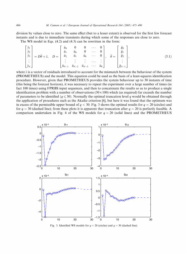
(PROMETHEUS) and the model. This equation could be used as the basis of a least-squares identificationprocedure. However, given that PROMETHEUS provides the system behaviour up to 30 instants of time

(this being the forecast horizon), it was necessary to repeat the experiment over a large number of times (in

fact 100 times) using FPRBS input sequences, and then to concatenate the results so as to produce a single

identification problem with a number of observations (30 · 100) which (as required) far exceeds the number

of parameters to be identified ðq6 30Þ. Normally the optimal truncation level q would be obtained through

the application of procedures such as the Akaike criterion [6], but here it was found that the optimum was

in excess of the permissible upper bound of q < 30. Fig. 3 shows the optimal results for q ¼ 20 (circles) and

for q ¼ 30 (dashed line); from these plots it is apparent that truncation after q ¼ 20 is perfectly feasible. Acomparison undertaken in Fig. 4 of the WS models for q ¼ 20 (solid lines) and the PROMETHEUS

0 10 20 30–2.5

–2

–1.5

–1

–0.5

0

0.5x 10–3 g11

0 10 20 30–4

–3

–2

–1

0

1x 10–3 g12

0 10 20 30

–4

–2

0

2x 10–4

g21

0 10 20 30–1.5

–1

–0.5

0

0.5

1

1.5x 10–4

g22

Fig. 3. Identified WS models for q ¼ 20 (circles) and q ¼ 30 (dashed line).

0 10 20 30–25

–20

–15

–10

–5

0

5y 1

1(k)

k0 10 20 30

–5

–4

–3

–2

–1

0

1

y 12(

k)

k

0 10 20 30–5

–4

–3

–2

–1

0

1

y 21(

k)

k0 10 20 30

–0.3

–0.2

–0.1

0

0.1

0.2

y 22(

k)

k

Fig. 4. Impulse responses: WS model (solid line), PROMETHEUS (dashed line).


impulse responses (dashed lines) obtained upon the application of orthogonal shocks, shows that with the

exception of the pair i ¼ 1, j ¼ 2, agreement is good, the differences reflecting the non-linear and time-

varying behaviour of PROMETHEUS. A more meaningful comparison would be to contrast the response

of the WS models (dashed lines) against that of PROMETHEUS (solid lines) for the same input sequences

and this is undertaken in Fig. 5 where two randomly selected FPRBS are applied, one for CCGT and the

other for WIND. Agreement here is seen to be very good and the plots provide convincing evidence as to

the suitability of the WS approximations.

The formulation of the optimisation problem of (3.14) requires the expected values and covariancematrices for hi. The former can be computed from (3.11) when vectors gTi are replaced by the vectors of the

elements of the identified WS shown in Fig. 3. Alternatively, both the expected values and covariance

matrices for hi can be computed from Monte Carlo simulations of (3.11) on PROMETHEUS; as explained

earlier, biðkÞ is to be taken to be zero. It is noted that such simulations will model the incremental effect of

the predicted shocks uiðkj0Þ and as such will include the effects of the random PROMETHEUS coefficients,

but not those of the exogenous variables. This is fortuitous because, depending on the size of the total

budget, the effects of exogenous variables could dominate the behaviour of the various performance

indicators thereby obscuring any beneficial effects that the policy of optimising the predicted allocationsuiðkj0Þ might have. It is emphasised that the purpose of the tool being developed is policy assessment, not

the minimization of the effect random exogenous variables (which after all could only be effected through

the use of feedback and would therefore concern a receding horizon implementation of the optimisation

strategy). The results of the Monte Carlo simulations are summarised below.

MT ~g11 �N�9:7249e� 3

�8:0158e� 2

� �;

2:9901e� 5 2:3382e� 4

2:3382e� 4 1:8340e� 3

� �� ; ð5:2Þ

0 10 20 30–200

–150

–100

–50

0

k

y 11(

k)

0 10 20 30–80

–60

–40

–20

0

k

y 12(

k)

0 10 20 30–20

–15

–10

–5

0

k

y 21(

k)

0 10 20 30–1.5

–1

–0.5

0

0.5

1

k

y 22(

k)

Fig. 5. Responses to FPRBS: WS model (solid line), PROMETHEUS (dashed line).


MT ~g12 �N�2:6021e� 2�1:9682e� 1

� �;

1:9301e � 4 1:4977e� 31:4977e � 3 1:1875e� 2

� �� ; ð5:3Þ

MT ~g21 �N�1:1327e� 3�9:4616e� 3

� �;

2:6544e � 7 2:1270e� 62:1270e � 6 1:7212e� 5

� �� ; ð5:4Þ

MT ~g22 �N�1:2517e� 4

�6:6997e� 4

� �;

1:3508e � 6 9:6789e� 6

9:6789e � 6 7:0022e� 5

� �� : ð5:5Þ

Introducing (5.2)–(5.4) into the static optimisation of (2.4), which can be implemented through the

formulation of (3.14) provided that that x1i and x2i are constrained to be equal to one another for all i,results in the optimal discounted input sequences shown in Fig. 6. The data for this figure, and for Figs. 7–9

was: A1 ¼ �2000, p1 ¼ 0:7, and A2 ¼ �200 with p2 being the probability that is being maximised. The

corresponding output sequences are shown in Fig. 7, where the results are shown as obtained from the WS

models (solid lines) as well as through PROMETHEUS (dashed lines) when this is used in its deterministic(expected values) form. The respective results for the dynamic formulation of (3.14) are shown in Figs. 8

and 9 and can be seen to be vastly different, despite the fact that the improvement in the probability that is

being maximised is somewhat modest (the static optimal was p2 ¼ 0:5646, and the dynamic optimal

p2 ¼ 0:5825, representing an improvement of 3.2%). The significant difference in input sequences is also

reflected in the resulting output sequences, and indeed the expected cumulative effect on EC, as computed

by PROMETHEUS, is )208.3 for the static formulation and )233.7 for the dynamic; these figures rep-

resent reductions (with respect to a baseline) on energy costs, and it is clear that the dynamic results

outperform (by about 12%) the static results.

0 5 10 15 20 25 300

2000

4000

6000

8000

10000

12000

u 1(k

)

0 5 10 15 20 25 300

500

1000

1500

2000

2500

k

u 2(k

)

Fig. 6. Inputs for static optimisation.

0 5 10 15 20 25 30–200

–150

–100

–50

0

y 1(k

)

0 5 10 15 20 25 30–14

–12

–10

–8

–6

–4

–2

0

k

y 2(k

)

Fig. 7. Outputs for static optimisation: WS (solid), PROMETHEUS (dashed).


The modest improvement in maximised probability can be made a great deal more significant (rising byabout 12% from 0.5646 for the static to 0.6311 for the dynamic) through the use of all degrees of freedom

that are available in the dynamic formulation. However this improvement is achieved through input

sequences that become very active towards the end of the forecast horizon. From a sustainable development

0 5 10 15 20 25 300

0.5

1

1.5

2

2.5

3

3.5x 104

u 1(k

)

0 5 10 15 20 25 300

2000

4000

6000

8000

10000

k

u 2(k

)

Fig. 8. Inputs for dynamic optimisation.

0 5 10 15 20 25 30–300

–250

–200

–150

–100

–50

0

50

y 1(k

)

0 5 10 15 20 25 30–25

–20

–15

–10

–5

0

5

k

y 2(k

)

Fig. 9. Outputs for dynamic optimisation: WS (solid), PROMETHEUS (dashed).


perspective, such behaviour may be less useful and for this reason the corresponding input and output

sequences will not be included in this paper.

Fig. 10 summarises the benefits possible in terms of the maximised probability p2 as the threshold A2 of

the cumulative sum of y2 is allowed to vary; the results for the static, dynamic with 2 degrees of freedom and

dynamic with all the degrees of freedom are plotted in dashed, solid and dotted lines respectively. Clearly

–250 –200 –150 –100 –50 0 50 1000.5

0.55

0.6

0.65

0.7

0.75

0.8

0.85

0.9

0.95

1

A2

max

p2

Fig. 10. The effect of A2 on the optimal values of p2.


the effect of A2 is significant and this is in direct contrast to the effects of p1 and A1 which are small; for this

reason no further plots have been included.Whereas the variation of the maximised p2 probability shown in Fig. 10 is continuous, the effect of this

variation on the optimising input trajectories for the dynamic formulation with 2 degrees of freedom is

0.5 0.55 0.6 0.65 0.7 0.75 0.8 0.85 0.9 0.95 10

0.5

1

1.5

2

2.5x 104

u 1(a

v,k<

10)

u 1(s

s)

0

1000

2000

3000

4000

5000

p2

u 2(a

v,k<

10)

u 2(s

s)

0.5 0.55 0.6 0.65 0.7 0.75 0.8 0.85 0.9 0.95 1

Fig. 11. The effect on input trajectories of variations in the optimal p2.


discontinuous, as shown in Fig. 11. Indeed, in particular ranges of values of p2 (e.g. between 0.92 and 0.955,or between 0.96 and 0.99), there is a complete reversal of strategy as illustrated by the switch in the values of

x2;i (dashed lines) and the average (over the ten forecast steps) values of x1;i (solid lines). As the probability

becomes large and hence the implied constraint on y2 becomes more stringent, so the optimisation tends to

place most of the emphasis of x2i which does not come into effect until the 11th forecast time instant. This

may be of no consequence in respect to the open-loop optimisation considered in this paper, but it is

conjectured that it would be of crucial importance in a receding horizon implementation of the optimisation

strategy.

6. Conclusions

The paper describes a dynamic extension to an earlier static optimisation approach to policy assessment

in sustainable development. This is achieved through the introduction of WS models and the derivation of

appropriate prediction equations that exploit the presence of discounting. The WS models and associated

statistics were derived through Monte Carlo simulations performed on a detailed and self-contained eco-

nomic model and are embedded into the optimisation problem to demonstrate the benefits of dynamicversus static modelling. As expected the improvements are significant and thus suggest the need for further

research into the effects of a receding horizon application of the optimisation strategy. It is envisaged that

this will require a re-examination of the objectives as well as careful examination of the difference between

open- and closed-loop results, especially in respect of respecting constraints (e.g. keeping actual cumulative

CO2 emissions below prescribed limits). It is expected that the requirement that steady state is reached

within the forecast horizon could be relaxed through the introduction of probabilistic inequality con-

straints; this in turn will allow the use of q ¼ 30, which could bring about better agreement between the WS

model and the PROMETHEUS results. It is also anticipated that techniques used in predictive control forthe guarantee of closed-loop stability will prove useful, but will have to be substantially modified before

they can be applied to meet objectives particular to sustainable development.

Acknowledgements

The European Commission is thanked for financial support under grant contract EVG1-2002-00082.

References

[1] N. Kouvaritakis, The ISPA meta-model, Technical report, ICCS, National Technical University of Athens, Greece, 2000.

[2] N. Kouvaritakis, (co-ordinator) European Commission project EVG1-CT-2002-00082: Methodologies for Integrating Impact

Assessment in the Field of Sustainable Development (MINIMA-SUD), 2002–2004.

[3] B. Kouvaritakis, M. Cannon, G. Huang, MPC as a tool for sustainable development integrated policy assessment, In: Proceedings

of the IFAC Conference on Control Systems Design, Bratislava, 2003.

[4] N. Kouvaritakis, Prometheus: A tool for the generation of stochastic information for key energy, environment and technology

variables, Technical report, ICCS, National Technical University of Athens, Greece, 2000.

[5] D.J. Cloud, B. Kouvaritakis, Statistical bounds on multivariable frequency response: An extension of the generalized Nyquist

criterion, Proceedings of IEE Part D 133 (3) (1986) 97–110.

[6] H. Akaike, New look at the statistical model identification, IEEE Transactions on Automatic Control 19 (6) (1974) 716–723.

[7] J.A. Rossiter, B. Kouvaritakis, Modelling and implicit modelling for predictive control, International Journal of Control 74 (11)

(2001) 1085–1095.

[8] M.S. Lobo, L. Vandenberghe, S.P. Boyd, H. Lebret, Applications of second-order cone programming, Linear Algebra and its

Applications 284 (1998) 193–228.

modelling and optimisation for sustainable development policy assessment

Documents