modelling and a tabu search solution for the slab reallocation

Modelling and a tabu search solution for the slab reallocation problem in the steel industry

Lixin Tanga*, Jiaxiang Luob and Jiyin Liuc

aLiaoning Key Laboratory of Manufacturing System and Logistics, The Logistics Institute, Northeastern University, Shenyang 110819,China; bSchool of Automation Science and Engineering, South China University of Technology, Guangzhou 510640, China; cTheLogistics Institute, Northeastern University, Shenyang, China; School of Business and Economics, Loughborough University,

Leicestershire, LE11 3TU, UK

(Received 3 May 2012; final version received 18 March 2013)

This paper considers a slab reallocation problem arising from operations planning in the steel industry. The probleminvolves reallocating steel slabs to customer orders to improve the utilisation of slabs and the level of customer satisfac-tion. It can be viewed as an extension of a multiple knapsack problem. We firstly formulate the problem as an integernonlinear programming (INLP) model. With variable replacement, the INLP model is then transformed into a mixed inte-ger linear programming (MILP) model, which can be solved to optimality by MILP optimisers for very small instances.To obtain satisfactory solutions efficiently for practical-sized instances, a heuristic algorithm based on tabu search (TS) isproposed. The algorithm employs multiple neighbourhoods including swap, insertion and ejection chain in local search,and adopts solution space decomposition to speed up computation. In the ejection chain neighbourhood, a new and moreeffective search method is also proposed to take advantage of the structural properties of the problem. Computationalexperiments on real data from an advanced iron and steel company in China show that the algorithm generates verygood results within a short time. Based on the model and solution approach, a decision support system has been devel-oped and implemented in the company.

Keywords: steel production; slab reallocation; tabu search; ejection chain neighbourhood; solution space decomposition

1. Introduction

Steel production consists of several main processing stages of iron making, steel making, casting, rolling and finishing,as shown in Figure 1. Slabs are produced on continuous casters in the casting stage and then rolled into coils throughhot rolling mills.

Slab production is planned based on customer orders and each slab matches a customer order in the plan. However,the slabs actually coming out of the steelmaking–casting process may not perfectly match with their customer ordersdue to the following reasons: (1) surplus slabs are compulsorily created for some orders to achieve the capacity require-ments of the steel-making furnace which must process fixed tonnes of molten steel at one time; (2) intermediate slabs,connecting two casts with different quality levels of molten steel or different geometrical dimensions in the castingstage, do not satisfy the required quality levels or dimension requirements of their orders since it is hard to control thequality and dimensions of these slabs by the casting technology; and (3) some orders are cancelled after the slabs forthem have been produced.

The unsatisfactory matching relationships between slabs and orders affect the company’s performance in a numberof ways: the level of customer satisfaction may be lowered because some orders may include non-first-choice slabs;steel material may be wasted as some slabs may need to be cut to satisfy the geometrical requirements of their orders;and the company’s profit may be reduced since customers usually pay a lower price for the surplus product weight overtheir requirement in accordance with the agreement between the customers and the company. While some matching rela-tionships between the slabs and their orders are not satisfactory, new orders are continuously arriving, which brings theprobability of improving the matching relationships to the slabs. Therefore, a natural idea for improving matching rela-tionships is to reallocate the slabs among all the orders on hand.

In this paper, the problem of reallocating slabs to orders is considered to optimise the matching relationships betweenslabs and orders. Since we need to adjust the matching relationship between the slabs and their orders based on theiroriginal matching relationships, the focus problem is named the slab reallocation problem, or the reallocating slabs to

*Corresponding author. Email: [email protected]

International Journal of Production Research, 2013Vol. 51, No. 14, 4405–4420, http://dx.doi.org/10.1080/00207543.2013.788796

� 2013 Taylor & Francis

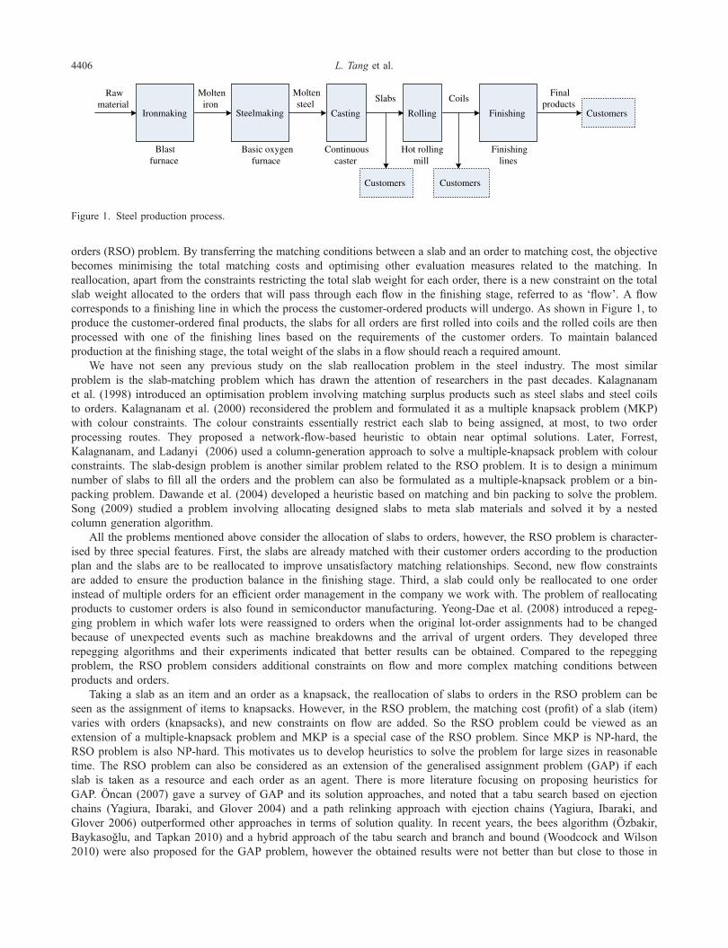
orders (RSO) problem. By transferring the matching conditions between a slab and an order to matching cost, the objectivebecomes minimising the total matching costs and optimising other evaluation measures related to the matching. Inreallocation, apart from the constraints restricting the total slab weight for each order, there is a new constraint on the totalslab weight allocated to the orders that will pass through each flow in the finishing stage, referred to as ‘flow’. A flowcorresponds to a finishing line in which the process the customer-ordered products will undergo. As shown in Figure 1, toproduce the customer-ordered final products, the slabs for all orders are first rolled into coils and the rolled coils are thenprocessed with one of the finishing lines based on the requirements of the customer orders. To maintain balancedproduction at the finishing stage, the total weight of the slabs in a flow should reach a required amount.

We have not seen any previous study on the slab reallocation problem in the steel industry. The most similarproblem is the slab-matching problem which has drawn the attention of researchers in the past decades. Kalagnanamet al. (1998) introduced an optimisation problem involving matching surplus products such as steel slabs and steel coilsto orders. Kalagnanam et al. (2000) reconsidered the problem and formulated it as a multiple knapsack problem (MKP)with colour constraints. The colour constraints essentially restrict each slab to being assigned, at most, to two orderprocessing routes. They proposed a network-flow-based heuristic to obtain near optimal solutions. Later, Forrest,Kalagnanam, and Ladanyi (2006) used a column-generation approach to solve a multiple-knapsack problem with colourconstraints. The slab-design problem is another similar problem related to the RSO problem. It is to design a minimumnumber of slabs to fill all the orders and the problem can also be formulated as a multiple-knapsack problem or a bin-packing problem. Dawande et al. (2004) developed a heuristic based on matching and bin packing to solve the problem.Song (2009) studied a problem involving allocating designed slabs to meta slab materials and solved it by a nestedcolumn generation algorithm.

All the problems mentioned above consider the allocation of slabs to orders, however, the RSO problem is character-ised by three special features. First, the slabs are already matched with their customer orders according to the productionplan and the slabs are to be reallocated to improve unsatisfactory matching relationships. Second, new flow constraintsare added to ensure the production balance in the finishing stage. Third, a slab could only be reallocated to one orderinstead of multiple orders for an efficient order management in the company we work with. The problem of reallocatingproducts to customer orders is also found in semiconductor manufacturing. Yeong-Dae et al. (2008) introduced a repeg-ging problem in which wafer lots were reassigned to orders when the original lot-order assignments had to be changedbecause of unexpected events such as machine breakdowns and the arrival of urgent orders. They developed threerepegging algorithms and their experiments indicated that better results can be obtained. Compared to the repeggingproblem, the RSO problem considers additional constraints on flow and more complex matching conditions betweenproducts and orders.

Taking a slab as an item and an order as a knapsack, the reallocation of slabs to orders in the RSO problem can beseen as the assignment of items to knapsacks. However, in the RSO problem, the matching cost (profit) of a slab (item)varies with orders (knapsacks), and new constraints on flow are added. So the RSO problem could be viewed as anextension of a multiple-knapsack problem and MKP is a special case of the RSO problem. Since MKP is NP-hard, theRSO problem is also NP-hard. This motivates us to develop heuristics to solve the problem for large sizes in reasonabletime. The RSO problem can also be considered as an extension of the generalised assignment problem (GAP) if eachslab is taken as a resource and each order as an agent. There is more literature focusing on proposing heuristics forGAP. Öncan (2007) gave a survey of GAP and its solution approaches, and noted that a tabu search based on ejectionchains (Yagiura, Ibaraki, and Glover 2004) and a path relinking approach with ejection chains (Yagiura, Ibaraki, andGlover 2006) outperformed other approaches in terms of solution quality. In recent years, the bees algorithm (Özbakir,Baykasoğlu, and Tapkan 2010) and a hybrid approach of the tabu search and branch and bound (Woodcock and Wilson2010) were also proposed for the GAP problem, however the obtained results were not better than but close to those in

Ironmaking Casting Rolling Finishing

Rawmaterial

Molteniron

Moltensteel

Slabs CoilsFinal

products

Customers Customers

Customers

Blastfurnace

Basic oxygenfurnace

Continuouscaster

Hot rollingmill

Finishinglines

Steelmaking

Figure 1. Steel production process.

4406 L. Tang et al.

Yagiura, Ibaraki, and Glover (2004, 2006). Considering the similarities and the differences among the RSO problem,MKP and GAP, we propose a tabu search approach with an ejection chain neighbourhood to solve the RSO problem.

In this paper we first formulate an integer nonlinear programming (INLP) model for the RSO problem and transformit into a mixed integer linear programming (MILP) model. A heuristic based on a tabu search with multiple neighbour-hoods defined by swap, insertion and ejection chain is developed to solve it. In the ejection chain neighbourhood, anew and more effective search method based on the shortest path is also proposed taking advantage of the structuralproperties of the problem. Moreover, the solution space decomposition strategy, which separates the slabs from theorders they have no possibility of matching, is adopted to speed up computation. Finally, a decision support system isimplemented based on the models and the proposed heuristic.

The rest of the article is organised as follows. Section 2 provides a detailed description of the RSO problem includ-ing the matching conditions of slabs and orders, the reallocation constraints and the components in the objective. Theinteger nonlinear programming model is presented and transformed into a mixed integer linear programming model inSection 3. In Section 4, a solution space decomposition strategy, multiple neighbourhoods and the tabu search algorithmare presented. The implementation issues are discussed and computational results are presented in Section 5. The slabreallocation decision support system based on the models and the proposed heuristic is introduced in Section 6.Concluding remarks are made in Section 7.

2. Problem description

The RSO problem is to reallocate slabs to orders in order to optimise the original matching relationships. The matchingconditions are first transferred to and quantified as matching costs which will then be minimised.

2.1 Transferring matching conditions of slabs and orders to matching costs

Most slabs are rectangle, others trapezoid, in shape. A slab i is characterised by a number of attributes: quality level(represented by steel grade SGi), widths at the two ends (twi and bwi, twi= bwi if slab i is rectangular), length (li), thick-ness (ti) and weight (wi). Slab i could be allocated to an order j if the slab meets all the order’s requirements.

(1) Quality level requirements:The steel grade of slab i should be the same as that required by order j, or be one of those with which the required

steel grade can be substituted. The substitution relationships among the steel grades are suggested by the materialexperts and are agreed upon by the customers in advance.

(2) Geometrical specification requirements:The width, length and weight of slab i should be in the ranges required by order j, with the width range being [SLBj,

SUBj], the length range being [LLBj, LUBj], the weight range being [WLBj, WUBj] and the extreme weight range being(0, WMBj]. If the width, length or weight of slab i is out of the range required by order j, the slab can still be allocatedto the order under the following situations: (1) the slab could be cut to the required size and weight if the cut-off weightdoes not exceed a maximum tonnage (MCW), for example, under our consideration MCW=5; or (2) the slab weightcan be divided into several units with each unit in the range of [WULBj, WUUBj] if the size of the slab is within thewidth, length and extreme weight ranges.

Obviously, slab cutting reduces slab utilisation and causes waste of steel material while steel grade substitutionreduces the level of customer satisfaction. A good match between a slab and an order should be the one without slabcutting or steel grade substitution. Notice that the matching conditions are cumbersome. So, to evaluate the matchbetween slab i and order j, a matching cost cij is defined as follows.

cij ¼ k1 maxfcw1ij; cw2ij; cw3ij; cw4ijg þ k2vij þ k3rij; if slab i is available to order jM ; otherwise

�(1)

where cw1ij, cw2ij, cw3ij and cw4ij are the cut-off weights as slab i is cut to width, length, weight and extreme weightrespectively, and vij is a quantified value of steel grade substitution, which is determined with practitioner experience.Considering that the original match between a slab and an order is not expected to change unless significant improve-ments can be made because the changes may cause extra logistics operations such as stock, an extra cost k3rij is addedto cij to avoid unnecessary changes of the original matching relationship of slab i and order j. Furthermore, we set cij toa very large number M if slab i is unavailable for order j.

International Journal of Production Research 4407

2.2 Reallocation constraints

(1) Each order j has a target weight Atj of slabs. It is rare to have the total weight of several slabs exactly equal to the

target weight. Thus, it is acceptable if the total slab weight allocated to the order is in a range of [Aminj ; Amax

j ], around

the target weight. Order j is said to be complete if the slab weight allocated to it is not less than Aminj , and is incomplete

otherwise. If the total weight of slabs allocated to order j is larger than Amaxj , it can also be accepted under the condition

that removing the lightest slab from those allocated to the order would make the order incomplete. Hence, in the modelformulation, the total weight of slabs allocated to order j is forced not to exceed Amin

j plus the minimum weight of slabs

allocated to order j.(2) As mentioned earlier, there is a restriction on the total slab weight allocated to the orders in each flow. In practi-

cal production, the equipment for the finishing operations cannot wait for materials, while materials can wait for equip-ment. So, to ensure the continuality of equipment running and to keep a balanced production, it is required that the totalslab weight for each flow k (k = 1, 2, …, K) should be at least Bk. There is also a guided upper bound for the total slabweight of each flow to limit the work-in-process inventory. As this is only a guide, the total weight may exceed it, buta penalty will be introduced for this.

(3) Slabs cannot be released from their originally matched orders if they are not reallocated to other orders. Thisactually requires that each slab must be allocated to an order. A slab is allowed to be reallocated to a new order, not theone to which it originally was matched, only if it does not violate the total weight restriction for the original order afterreallocation. If there is no such order for a slab, the slab must be allocated to the order to which it was originallymatched. Therefore, an order originally having surplus slabs may still remain so after reallocation. In this case, the orderis permitted to have surplus slabs and can disobey the constraint on slab weight for the order.

2.3 Aim and objectives

The goal of the RSO problem is to optimise the matching relationships between slabs and orders by reallocating theslabs to orders. The following factors are included to evaluate the reallocation of slabs: the number of incompleteorders, the amount of slab weight shortage in orders, the amount of surplus slab weight in orders, the sum of matchingcosts, the priority of orders with reallocated slabs and the amount of slab weight beyond the guided upper bound forflows.

The orders having the following features are given higher priority. (1) Priority is given to the orders with specialrequirements, and the slab allocation to them should be made first. (2) Priority is given to urgent orders with tight slacktimes over others where the slack time of an order is the time period from the current time to the latest start time to rollthe slabs for the order. (3) Priority is given to the orders in a later state. Here, a state of an order indicates the process-ing stage of handling the order. There are three states, state S1, S2 and S3, indicating that the molten steel, slabs androlled coils for an order have been respectively produced according to production plan. The orders in later states aregiven priority over the ones in earlier states. (4) Priority is given to the orders of a special type. According to a marketstrategy of a company to customers, type A1, A2 and A3 of orders indicate three kinds of strategic customers and typeA1 orders have the highest priority. The above four factors are quantified and integrated into a priority prize usingweighing coefficients, which is further explained in Section 3.4.

Using weighing coefficients and transferring the evaluation factors to quantified prizes or penalties, a single objectiveof the RSO problem is formed, which consists of the following components: minimising the sum of matching costs,maximising the prize for matching slabs to orders with priority, minimising the number of incomplete orders and mini-mising the penalties for the slab weight shortage in orders, the surplus slab weight in orders and the slab weight beyondthe guided upper value for flows.

3. Problem formulation

3.1 Notation

Parameters:I= {1, 2, …, N}: the set of N slabs to be reallocated;J= {1, 2, …, M}: the set of M orders to be considered;i index of slabs (i 2 I);j index of orders (j 2 J);k index of flows (k= 1, 2, …, K);

4408 L. Tang et al.

Oi the order to which slab i was originally allocated;ai the weight of slab i;Rj the quantified priority of order j;Aminj the minimum total slab weight required by order j;

Amaxj the maximum total slab weight required by order j that should preferably not exceed;

Pj the penalty if order j is incomplete;cij the matching cost when slab i is allocated to order j;Hk the set of orders in flow k;Bk the required minimum total slab weight for flow k;Tk the guided upper bound for the total slab weight of flow k;F1 the weighing coefficient of matching costs;F2 the weighing coefficient of the prizes for orders with priority;F3 the weighing coefficient of the penalties for incomplete orders;F4 the weighing coefficient of penalties for the slab weight shortage in orders;F4′ the weighing coefficient of penalties for surplus slab weight of orders;F5 the weighing coefficient of penalties for the slab weight beyond the guided upper limits of flows;UW a slab weight limit, beyond which the penalties for the slab weight shortage in orders is set at the same;u1 the unit penalty for the slab weight shortage in orders;u2 the unit penalty for the slab weight beyond the weight upper bound of orders;L a very large number.Variables:

xij ¼ 1; if slab i is reallocated to order j;0; otherwise:

�

dj ¼ 1; if at least one slab allocated to other orders is now reallocated to order j;0; otherwise:

�

3.2 The model

With the above parameters and variables, the RSO problem can be formulated as the model below.

Minimise

Z ¼ F1

XMj¼1

XNi¼1

cijxij � F2

XMj¼1

XNi¼1

Rjxij þ F3

XMj¼1

Pjsgn max Aminj �

XNi¼1

aixij; 0

( ) !þ F4

XMj¼1

u1 min max 0;Aminj �

XNi¼1

aixij

( );UW

( )

þ F 04

XMj¼1

u2 max 0;XNi¼1

aixij � Amaxj

( )þ F5

XKk¼1

Xj2Hk

maxXNi¼1

aixij � Tk ; 0

( )

Subject to

XMj¼1

xij ¼ 1; i ¼ 1; 2; . . . ;N (2)

Xj2Hk

XNi¼1

aixij � Bk ; k ¼ 1; 2; . . . ;K (3)


XNi¼1;Oi–j

xij � Ldj; j ¼ 1; 2; . . . ;M (4)

dj �XN

i¼1;Oi–j

xij; j ¼ 1; 2; . . . ;M (5)

XNi0¼1

ai0xi0j � Aminj þ ai þ L(1� xij)þ L(1� dj); i ¼ 1; 2; . . . ;N ; j ¼ 1; 2; . . . ;M (6)

xij; dj 2 f0; 1g; i ¼ 1; 2; . . . ;N ; j ¼ 1; 2; . . . ;M (7)

The objective function includes six components.PM

j¼1

PNi¼1 cijxij is the sum of matching costs.

PMj¼1

PNi¼1 Rjxij is

the sum of prizes for reallocating slabs to orders with priority. As the whole objective is to be minimised, a negative

sign is added to this prize term.PM

j¼1 Pjsgn(maxfAminj �PN

i¼1 aixij; 0g) is the sum of penalties for incomplete orders.PMj¼1 u1 minfmaxf0;Amin

j �PNi¼1 aixijg;UWg is the sum of penalties for the slab weight shortages in all orders. Consid-

ering that many orders, especially new ones arriving to the order pool, lack slabs, the penalty for each order is bound

by u1UW.PM

j¼1 u2 maxf0;PNi¼1 aixij � Amax

j g is the sum of penalties for the surplus slab weight in orders.PKk¼1

Pj2Hk

maxfPNi¼1 aixij � Tk ; 0g is the sum of penalties for the slab weight beyond the guided upper limits of

flows.Constraints (2) require that each slab must be allocated to an order. Constraints (3) state that the total slab weight

for each flow k should be at least Bk (k = 1, 2, …, K). Constraints (4) and (5) define the variable dj which indicateswhether there are new slabs allocated to order j. Constraints (6) indicate the total slab weight for an order is less thanthe minimum acceptable slab weight plus each slab reallocated to the order. If no new slab is allocated to an order, theconstraint for this order becomes redundant. Constraints (7) set the ranges of the variable values. It can be seen fromthe model that the original allocation determines the variables in constraints (4) and (5), and further has an influence onconstraints (7). So, the optimal solution of the model is related to the original allocation of slabs, which distinguishesthe slab reallocation problem from the general allocation or assignment problem.

The problem can be viewed as an extension of an MKP. However, in this problem, the profit of an item (slab) varieswith knapsacks (orders), which can be seen from the first part of the objective, and new flow constraints, constraints(3), are added. The problem can also be taken as an extension of a GAP. But the resources of a task (slab) occupyingdifferent agents (orders) are the same, which can be seen from constraints (6), and also the problem involves new con-straints, constraints (3), on flows.

3.3 Linearised model

The model is nonlinear because of the terms such as max{x, y} and min{x, y}. By introducing new variables and newconstraints, the model could be transformed to a linear one. A term in the form of max{x, y} in the objective can bereplaced by a new variable w with additional constraints w � x and w � y. A term in the form of min{x, y} can bereplaced by a variable v. To achieve the purpose of the original formulation, a new 0–1 variable q and the followingadditional constraints are introduced: vþ L(1� q) � x; vþ Lq � y; x� y � L(1� q) and y� x � Lq. In this way, we

can replace the expression sgn(maxfAminj �PN

i¼1 aixij; 0g) by a variable yj;minfmaxf0;Aminj �PN

i¼1 aixijg;UWg by

wj; and maxf0;PNi¼1 aixij � Amax

j g by vj; andmaxfPj2Hk

PNi¼1 aixij � Tk ; 0g by sk. The model can be transformed into

the following linear one.

Minimise Z ¼XMj¼1

XNi¼1

(F1cij � F2Rj)xij þXMj¼1

F3Pjyj þXMj¼1

F4u1wj þXMj¼1

F 04u2vj þ

XKk¼1

F5sk (8)

Subject to constraints (2) to (7) and to the following constraints:

4410 L. Tang et al.

Aminj �

XNi¼1

aixij � Lyj; j ¼ 1; 2; . . . ;M (9)

wj � qjUW � 0; j ¼ 1; 2; . . . ;M (10)

Aminj �

XNi¼1

aixij � UW � Lqj; j ¼ 1; 2; � � � ;M (11)

Aminj �

XNi¼1

aixij � Lqj � wj; j ¼ 1; 2; � � � ;M (12)

XNi¼1

aixij � vj � Amaxj ; j ¼ 1; 2; . . . ;M (13)

Xj2Hk

XNi¼1

aixij � sk � Tk ; k ¼ 1; 2; . . . ;K; (14)

0 � wj � UW ; vj � 0; sk � 0; k ¼ 1; 2; . . . ;K; j ¼ 1; 2; . . . ;M (15)

yj; qj 2 f0; 1g; j ¼ 1; 2; . . . ;M (16)

The original nonlinear model has NM xij variables and M δj variables while the equivalent mixed integer linear pro-gramming model adds M new variables for each variable type yj, wj, vj and qj and K sk variables. If all the modelparameters are given, the model could be solved to optimality by an MILP optimiser in reasonable time for smallinstances.

3.4 Model parameter setting

In the model, an important matter is to set the model parameters including weighting coefficients and all the quantifiedprizes and penalties. To ensure the model’s effectiveness, all parameters should reflect real situations in production. Sowe have worked with practitioners in the company we work with to tune these parameters iteratively. First, the parame-ters were set roughly according to the suggestions of practitioners. Then we solved the model and provided the resultsto the practitioners. The practitioners gave their feedback, according to which we modified the parameters and solvedthe model again. The process was repeated until the practitioners were satisfied with the results obtained using the fol-lowing parameters.

(1) Matching cost: cij = k1max{cw1ij, cw2ij, cw3ij, cw4ij} + k2vij+ k3rij. The parameters are set as follows:k1 = k2 = k3 = 1; vij= ld�Cv where ld = 10 and Cv is the grade difference between the steel grade of slab i and thatrequired by order j; rij= 50 if j=Oi, 0 otherwise.

(2) Quantified priority of order j :Rj ¼ Rj1 þ Rj2 þ Rj3 þ Rj4.

Rj1 ¼ p1; if order j is special;0; otherwise;

�

Rj2 is set to be a step function of slack time st (days) as follows:


Rj2 ¼

p2; if st\0;p3; if st ¼ 0;p4; if st ¼ 1;p5; if st ¼ 2;p6; if st ¼ 3;0; if st � 4:

8>>>>>><>>>>>>:

Rj3 = p7, p8 and p9 for states S1, S2 and S3 of orders respectively;Rj4 = p10, p11 and p12 for types A1, A2 and A3 of orders respectively.

All the prizes, p1 to p12, are measured in terms of profit on reallocating slabs to priority orders. For example,p10 = 50 means that a slab’s match to an order with type A1 is converted into ¥50 of additional profit. In a similar way,the values of all other parameters related to order priority are set and shown in Table 1. To improve the flexibility ofthe algorithm, they are adjustable in implementation.

(3) Other coefficients are as follows: (a) the penalty for order j if it is incomplete: Pj= 50, (b) the unit costs: u1 = 1and u2 = 10, where u2 is larger than u1 as it is common that most orders lack slabs, (c) weighting coefficientsF1 =F2 =F3 =F4 =F4′ =F5 = 1, and (d) UW= 50.

The values of the parameters imply the importance of the factors to evaluate the matches between slabs and orders.Since they are adjustable in implementation, the importance of the factors could be changed according to market needs.

4. The solving approach based on tabu search

The fact that the RSO problem is NP-hard implies that it is difficult to find its optimal solutions within a reasonable timeand a heuristic is necessary to generate near-optimal solutions in a very short time. Therefore, a heuristic based on tabusearch (TS) is designed. There are three considerations for the heuristic: (1) the slabs and orders can be grouped into dif-ferent parts according to their steel grades, which could be used to speed up computation, (2) all the slabs are originallyallocated to orders, and their matching relationships comprise a feasible solution to the problem and could be utilised inthe algorithm, and (3) as it has been mentioned, an order is permitted to have surplus slabs and can disobey the slabweight constraint if all the slabs reallocated to it were originally matched with it. Based on these considerations, the TS-based heuristic designed for the RSO problem includes three main steps. In the first step, the solution space is decom-posed into different parts according to steel grades. In the second step, TS is used to search for near-optimal solutions ineach solution space part, utilising the original matching relationships between slabs and orders to generate an initial solu-tion while allowing the weight of slabs reallocated to each order to be larger than required during the search since not allorders need to obey the slab weight constraints. In the last step, the resulting solution is modified to a feasible one.

4.1 Domain decomposition of the solution space

As mentioned in Section 2, the matching condition on quality level requires that the slab’s steel grade should be thesame as or could substitute for that required by its matched order. It is true that steel grades can be grouped into dis-jointed subsets such that no substitution can be made between any two steel grades from distinct subsets in steel produc-tion. The slabs and orders can also be grouped into distinct subsets according to steel grades, as show in Figure 2,where G groups of slabs and orders are assumed.

Distinct subsets of slabs and orders make it possible to decompose the objective function, slab allocation constraints(2) and weight constraints (3) into distinct parts accordingly. However, the orders from different subsets may belong to thesame flow, so the flow constraints cannot be decomposed in the same way. Considering that fast algorithms and satisfac-tory solutions are often sought in real application, we turn to decompose the flow constraints approximately as follows.

Table 1. Values of parameters in Rj.

Parameters

Rj1 Rj2 Rj3 Rj4

p1 p2 p3 p4 p5 p6 p7 p8 p9 p10 p11 p12

Profit (¥) 10 5000 4000 2000 800 200 1000 800 0 50 0 0

4412 L. Tang et al.

Xj2Hkg

XNi¼1

aixij � Bkg; g ¼ 1; 2; . . . ;G; k ¼ 1; 2; . . . ;K: (17)

where Hkg is the subset of orders with flow k in group g and Bkg is the lower limit on slab weight for flow k in groupg. The guided upper limit Tk for flow k is also decomposed into G parts as Tkg is the one for group g. Obviously, Bkg

and Tkg satisfy the following constraints.

XGg¼1

Bkg ¼ Bk; k ¼ 1; 2; . . . ;K: (18)

XGg¼1

Tkg ¼ Tk ; k ¼ 1; 2; . . . ;K: (19)

So, the solution space of the RSO problem is approximately divided into G different parts. The TS described insubsection 4.2 could be carried out G times and each time only one group of slabs and orders is considered. Thedecomposition makes the size of the instance solved each time by the TS much smaller, which is helpful in reducingthe total computation time. The feasible solution space after the decomposition may be reduced because of the addi-tional flow constraints for each group. However, to achieve fast algorithms and seek satisfactory solutions in a shorttime, such approximation decomposition may be worthwhile. The depth of decomposition approximation is affected bythe values of Bkg and Tkg since they determine the reduced feasible solution space. To set appropriate values for the twoparameters, we utilise the original matching relationships and the details are described in Section 4.3.

4.2 The main components of TS

4.2.1 Initial solution

Usually, there are advantages if the initial solution for TS is of good quality. Obviously, the original matching relation-ships of slabs and orders comprise a feasible solution to the RSO problem in spite of some matching relationships beingunsatisfactory and some orders having surplus slabs. Based on this, three heuristics have been constructed to generateinitial solutions by utilising the original feasible matching relationships. The first one reallocates only the surplus slabsof orders. The second one gradually releases and reallocates parts of slabs according to reference costs. The third onereleases and reallocates all the slabs according to reference costs. For slab i and order j, the reference cost is defined as:

c0ij ¼ F1cij � F2Rj þ F4u1 minfmaxf0;Aminj � Ajg;UWg þ F 0

4u2 maxf0;Aj � Amaxj g (20)

where Aj denotes the total weight of slabs currently allocated to order j. c0ij denotes the contribution to the objective ifslab i is allocated to order j. The contribution does not include the penalties for incomplete orders since it does notmean much as most orders are incomplete during the reallocation. Besides, it does not include the penalties for the slabweight beyond the guided upper limits of flows since a single matching relationship should not be responsible for theslab weight beyond the guided upper limits of flows. Computational test shows that the best heuristic is the second one,which is described as follows. Let ~I and ~J respectively denote the slab and order subsets considered.

Steel grade subset 1

Steel grade subset 2

Steel grade subset G

Slab subset 1

Order subset 1

All steel grades

Slab subset 2

Order subset 2

Slab subset G

Order subset G

Figure 2. Group slabs and orders into different subsets according to steel grades.


Step 1. Sort the orders in ~J in decreasing quantified priority as [1], … [j~J j];Step 2. (Release surplus slabs from orders) For order j= 1 to j~J j: if order [j] has surplus slabs, repeatedly select a

slab randomly and release it from order [j] as long as the order is still complete and the flow constraints arestill satisfied.

Step 3. (Release slabs according to reference cost)Let Lcost1 =max{c0ij; i 2 ~I ; j 2 ~J}-D1 where D1 is a predetermined parameter. Set i= 1.While (Lcost1 � 0)

While (i � j~I j)Let j=Oi, release slab i if c0ij � Lcost1 and the flow constraints are stillsatisfied after release. Set i= i+1.

EndSet Lcost1 = Lcost1-D1 and i= 1.

End

Step 4. (Reallocate slabs to orders)Set Lcost2 =D2 where D2 is a predetermined parameter. Set j= 1 and i= 1.While (Lcost2 <max{c0ij; i 2 ~I ; j 2 ~J}+D2)While (j � j~J j)

While (order [j] is incomplete and i � j~I j)If slab i is unallocated and c0i½j� � Lcost2, allocate it to order [j].

Set i= i+1.EndSet j= j+1 and i= 1.EndSet Lcost2 = Lcost2 +Δ2 and j= 1.

End

Step 5. (Modifying procedure) For i= 1 to j~I j: if slab i is new to its matched order which has surplus slabs or if slab i isreleased but not reallocated to any order, reallocate it to its original order Oi. Repeat this step until no such a slab isfound.

First, the surplus slabs on orders are released in Step 2. Second, each slab i, selected by c0ij � Lcost1, is releasedfrom its order j in the stage identified by Lcost1 if the flow constraints are not violated. Third, each released slab i, sat-isfying c0i½j� � Lcost2, is reallocated to order [j] in the stage identified by Lcost2. Lastly, the solution obtained is made

feasible in Step 5. Since D1 and D2 control the values of Lcost1 and Lcost2, they further control the numbers of stagesand the speeds of releasing and reallocating slabs. If D1[ maxfc0ij; i 2 ~I ; j 2 ~Jg, all possible slabs are released at the

first stage. If D2[ maxfc0ij; i 2 ~I ; j 2 ~Jg, the reallocation of slabs are also completed in the first stage. With smaller val-

ues of D1 and D2, the heuristic is more likely to release the slabs with unsatisfactory matching in the current solutionthan those with satisfactory matching and is more likely to get satisfactory matching than unsatisfactory matching in thereallocation of slabs to orders. However, too small of values for D1 and D2 will increase the computation burden. Inour implementation, the values of D1 and D2 are set by experiments.

4.2.2 Local search and basic neighbourhoods

Local search starts its search from an initial solution S and replaces the current solution with a better solution in itsneighbourhood N(S) repeatedly until no better solution is found in N(S). The resulting solution S is local optimal. Swapneighbourhood Nswap and insertion neighbourhood Ninsertion are usually used in local searches for their simplicity andeffectiveness. For the RSO problem, Nswap(S) is the solution subset including all the solutions obtained from S byexchanging the allocations of two slabs and Ninsertion(S) is the solution subset including all the solutions obtained from Sby changing the allocation of one slab. Besides the two neighbourhoods, ejection chain neighbourhood, a large neigh-bourhood, is also adopted to improve the solution quality for the problem considered and is described in Section 4.2.3.

4.2.3 Ejection chain neighbourhood and its search method

To describe ejection chain move and neighbourhood more clearly, we describe them through MKP. For an MKP with nitems and m knapsacks, an ejection chain move is a series of shift moves of items, denoted as the sequence of the items

4414 L. Tang et al.

involved (i0, i1, …, il). For any two adjacent items, the succeeding item is always shifted from its current knapsack to thepreceding item’s knapsack. The first item i0 is shifted to an arbitrary knapsack. Based on ejection chain move, the ejectionchain neighbourhood is defined as the set of solutions S0 obtained from the current solution S by an ejection chain move.

The neighbourhood size equals (m� 1)Pn

l¼1ln

� �, which is very large. So, Yagiura, Ibaraki, and Glover (2004)

restricted the neighbourhood search and proposed an algorithm to search in part of the neighbourhood. In the algorithmthe best neighbour is found through searching guided by the information obtained via Lagrangian Relaxation.

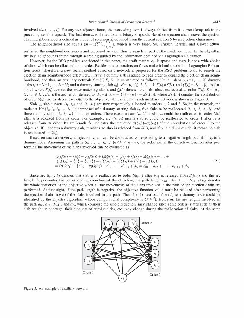
However, for the RSO problem considered in this paper, the profit matrix, cij, is sparse and there is not a wide choiceof slabs which can be allocated to an order. Besides, the constraints on flows make it hard to obtain a Lagrangian Relaxa-tion result. Therefore, a new search method based on a network is proposed for the RSO problem to try to search theejection chain neighbourhood effectively. Firstly, a dummy slab is added to each order to expand the ejection chain neigh-bourhood, and then an auxiliary network G = {V, E, D} is constructed as follows. V= {all slabs il, l= 1, …, N; dummyslabs il, l=N + 1, …, N +M; and a dummy starting slab i0}. E = {(il, ih): il, ih 2 V, S(il) ≠ S(ih), and Q(il) + {ih}�{il} is fea-sible} where S(il) denotes the order matching slab il and Q(il) denotes the slab subset reallocated to order S(il). D = {dlh:(il, ih) 2 E}. dlh is the arc length defined as dlh= z(Q(il) � {il} + {ih}) � z(Q(il)), where z(Q(il)) denotes the contributionof order S(il) and its slab subset Q(il) to the objective. An example of such auxiliary network is shown in Figure 3.

Slab i5, slab subsets {i1, i2} and {i3, i4} are now respectively allocated to orders 1, 2 and 3. So, in the network, thenode set V= {i0, i1, i2, …, i8} is composed of a dummy starting slab i0, five slabs to be reallocated {i1, i2, i3, i4, i5} andthree dummy slabs {i6, i7, i8} for three orders. There exists an arc (il, ih) if slab ih could be reallocated to order S(il)after il is released from its order. For example, arc (i3, i5) means slab i3 could be reallocated to order 1 after i5 isreleased from its order. Its arc length d35 indicates the reduction z({i3})�z({i5}) of the contribution of order 1 to theobjective. If il denotes a dummy slab, it means no slab is released from S(il), and if ih is a dummy slab, it means no slabis reallocated to S(il).

Based on such a network, an ejection chain can be constructed corresponding to a negative length path from i0 to adummy node. Assuming the path is (i0, i1, …, il, ih) (n< h � n +m), the reduction in the objective function after per-forming the movement of the slabs involved can be evaluated as

(z(Q(i1)� fiig)� z(Q(i1))þ (z(Q(i2)� fi2g þ fi1g)� z(Q(i2))þ . . .þ(z(Q(il)� filg þ fil�1g)� z(Q(il))þ (z(Q(ih)þ filg)� z(Q(ih))¼ (z(Q(i1)� fi1g)� z(Q(i1))þ d12 . . .þ dl�1;l þ dlh ¼ d01 þ d12 þ . . .þ dl�1;l þ dlh

(21)

Since arc (il�1, il) denotes that slab il is reallocated to order S(il�1) after il�1 is released from S(il�1) and the arclength dl�1,l denotes the corresponding reduction of the objective, the path length d01 + d12 +…+ dl�1, l+ dlh denotesthe whole reduction of the objective when all the movements of the slabs involved in the path or the ejection chain areperformed. At first sight, if the path length is negative, the objective function value must be reduced after performingthe ejection chain move of the slabs involved in the path. Then the shortest path from i0 to a dummy node could beidentified by the Dijkstra algorithm, whose computational complexity is O(|V|2). However, the arc lengths involved inthe path d01, d12, dl�1, l and dlh, which compose the whole reduction, may change since some orders’ states such as theirslab weight in shortage, their amounts of surplus slabs, etc. may change during the reallocation of slabs. At the same

i5

i8

i3

i4

i2i1

i0

i7

i6

Order 1

Order 2

Order 3

Figure 3. An example of auxiliary network.


time, the Dijkstra algorithm does not always yield optimal results if there are negative arc lengths in the network. Forthese two reasons, the following search strategy is adopted to search for an improved ejection chain: (1) Adopt the Dijk-stra algorithm repeatedly to search for the shortest path from i0 to each dummy node; (2) Sort the paths by increasingorder of their lengths; (3) Beginning from the first path sorted, check whether the objective is improved when the ejec-tion chain move of the slabs involved in the path is performed. Repeat the check procedure until the first improved ejec-tion chain is found or all the paths with negative lengths have been checked.

4.3 The whole tabu search approach

As mentioned in Section 4.1, the TS-based heuristic includes three stages: the solution space of the RSO problem isdecomposed into different parts in the first stage; then in each solution space part, the TS is adopted to search for bettersolutions in the second stage, allowing the weight of slabs reallocated to each order to be larger than required during thesearch since not all orders need to obey the slab weight constraints; and the final solution is modified to obtain a feasibleone after all the solution space parts are searched in the last stage. During the search in each solution space part, TS isapplied to solve the sub-instance composed of the slabs and orders in the corresponding group and the involved slabs andorders are said to be active. For TS, aside from the initial solution generation method and local search we have describedin the previous section, another important component is the tabu list. In the tabu list of the implementation of TS for theproblem, we record the slabs, which are involved in the current swap move. All the solutions involving a slab in the tabulist are tabooed during the swap neighbourhood search. What’s more, to encourage the search to work in a feasiblesolution space, all moves involved in the neighbourhood search are restricted in the following ways: moves which willcause the current solution to violate the flow constraints or will make a feasible solution into an infeasible one are notpermitted. We set x0ij = 1 if j=Oi, 0 otherwise; set xij = 1 if slab i is reallocated to order j, 0 otherwise; and let ~I and ~Jdenote the active slab and order subsets respectively. The heuristic based on TS is as follows.

Step 1. Group slabs and orders into G groups according to their steel grades. For each group g (g = 1, 2, …, G), letIg and Jg denote the slab and order subsets respectively. Set g = 1.

Step 2. Set ~I ¼ Ig and ~J ¼ Jg. Set Bkg=Bk �Pj2 [g�1

h¼1Hkh

Pi2I aixij �

Pj2 [G

h¼gþ1Hkh

Pi2I aix

0ij and

Tkg ¼ Tk �P

j2 [g�1

h¼1Hkh

Pi2I aixij �

Pj2 [G

h¼gþ1Hkh

Pi2I aix

0ij: Generate initial allocation Sc using the heuristic

presented in Section 4.2.1. Set Sb = Sc, iteration number Itr = 0 and number of iterations without improvementoutItr= 0. Let tabu list T = Ø.

Step 3. Search the best non-tabooed swap (SWAP) and the best tabooed swap (TSWAP) in the swap neighbourhoodof Sc. Perform SWAP and TSWAP on the current solution Sc and solutions Snt and St are obtainedrespectively.

Step 4. (Uses of aspiration level function) If Z(St) < Z(Sb) and Z(St) < Z(Snt), set Sb= St and Sc= St. Otherwise setSc= Snt, update Sb= Snt if Z(Sb) > Z(Snt). Move the slabs involved in SWAP if Sc= Snt or in TSWAP if Sc= Stto tabu list T and release the slabs which have been tabooed for Tl (tabu length) iterations. If Sb isimproved, set outItr = 0.

Step 5. (Insertion) Search and perform the best insertion in the insertion neighbourhood of Sc and solution Sit isobtained. Set Sc= Sit if Z(Sit) < Z(Sc) and set Sb= Sit if Z(Sit) < Z(Sb). If Sb is improved, set outItr= 0.

Step 6. (Ejection chain) The search in ejection chain neighbourhood, which has been presented in Section 4.2.3, is acti-vated after outItr is larger than Tr for the first time. Update Sc and Sb if possible. If Sb is improved, set outItr = 0.

Step 7. (Stopping criterion) Set Itr = Itr + 1 and outItr= outItr + 1. If Itr >maxItr or outItr >maxoutItr, the search ter-minates for group g, update xij and set g= g+ 1. Otherwise return to Step 3.

Step 8. Return to Step 2 if g � G, otherwise modify the final solution, denoted by xij, to a feasible one through themodifying procedure descried in the initial solution generation method and terminate the algorithm.

5. Algorithm implementation and computational experiment

The algorithm is programmed in C++ and executed on an i5–2.67G personal computer. The parameters for the heuristicare set as: D1 = 50, D2 = 50, tabu list length Tl = 7, maxItr = 100, maxoutItr = 20 and Tr= 10. Twenty sets of data are col-lected from real production to test the algorithms. To verify the algorithm efficiency and the model effectiveness, threeexperiments have been carried out as reported below.

4416 L. Tang et al.

(1) Comparisons of different versions of the algorithms.The objective function values obtained by the algorithms are transferred to relative measures with 1þ jZ�Z�j

jZ�j where Zis the objective value compared and Z� is the best one among them. The computational results are shown in Table 2. Inthe table, ‘TS’ and ‘TS-I’ respectively denote the TS with swap neighbourhood and the TS with swap and insertionneighbourhoods. Both TS-IC and TS-ILC adapt swap, insertion and ejection chain neighbourhoods, but the ejectionchain in TS-IC is constructed by the Dijkstra algorithm while in TS-ILC it is constructed by selecting slabs randomlyfrom orders.

It can be seen from Table 2 that the TS-IC algorithm performs best. The results indicate that the ejection chain couldhelp the algorithm find better solutions. Although TS-IC has a longer computation time than the others, the longest com-putation time is about 2 minutes and is acceptable in real production.

(2) Comparisons of the results obtained by TS-IC and an MILP solver for small-sized instances.An MILP solver, Cplex, is used to solve small-sized instances. For most instances, the MILP solver could obtain

optimal solutions in a very short time, as shown in column ‘MILP solver’ in Table 3. However, the solver, even run bya high-configuration computer, cannot handle instances 14 and 17 as they have too many variables and constraints.Compared with the MILP solver, the TS-IC algorithm could obtain near-optimal solutions for these instances, whichindicates the effectiveness of the algorithm.

(3) Comparison of the results obtained by TS-IC with the original matches.The following major factors are selected to evaluate the performance of the new matches obtained by the TS-IC

algorithm: the total number of slabs needed to be cut (CN), the total cut-off slab weight (CW), the numbers of completeorders (FON) and complete urgent orders (UFON), and the total surplus slab weight of orders (SW). The improvementby the TS-IC and the values of the original matches for each factor are presented in Table 4.

The results obtained by our approach represent considerable improvements over the original matches in the measuresconsidered. On average, the cut-off slab weight and the number of slabs needed to be cut are reduced by 26.67% and2.25% respectively, the numbers of complete orders and the complete urgent orders are increased by 6.36% and 12.63%respectively, and the total surplus slab weight is reduced by 28.84%. These improvements have positive consequencesfor the company and verify the model effectiveness. First, less cut-off slab weight and a smaller number of slabs need-ing to be cut reduce the burden of the cut machines as well as save resources. Second, the increased numbers of com-plete orders and complete urgent orders imply a better delivery performance and a higher customer satisfaction level.Third, the decreased total surplus slab weight for orders helps to make better use of slabs.

Table 2. Results of different algorithms.

No.Problem size

Transferred values Computation time (s)

(slabs � orders) TS-IC TS-ILC TS-I TS TS-IC TS-ILC TS-I TS

1 932 � 3865 1.0000 1.0912 1.0911 1.1053 61.50 31.42 27.41 30.672 800 � 3460 1.0000 1.2026 1.2026 1.2150 59.73 22.65 22.25 23.813 936 � 3367 1.0000 1.1137 1.1137 1.1138 52.93 26.90 23.48 26.104 998 � 3407 1.0000 1.0429 1.0447 1.0448 60.25 24.76 23.88 23.825 986 � 3438 1.0000 1.0289 1.0289 1.0410 49.86 27.41 23.21 26.576 613 � 3384 1.0000 1.0756 1.0672 1.0915 36.17 19.98 19.33 21.347 1021 � 3253 1.0000 1.0450 1.0435 1.0527 48.29 22.14 20.78 23.658 1040 � 3240 1.0000 1.0680 1.0661 1.0657 45.90 24.01 21.40 22.269 706 � 3191 1.0000 1.0392 1.0393 1.0546 50.22 19.48 18.47 19.1610 1017 � 3190 1.0000 1.0375 1.0378 1.0406 46.22 21.98 20.48 20.3711 990 � 3010 1.0000 1.0440 1.0427 1.0528 64.00 20.37 19.17 20.5812 899 � 3294 1.0000 1.0630 1.0612 1.0714 39.68 49.78 22.98 22.6713 1121 � 3524 1.0000 1.0727 1.0705 1.0706 75.73 56.72 27.30 29.8914 1105 � 4001 1.0000 1.0945 1.0962 1.0990 77.77 70.98 33.40 33.9815 1188 � 4057 1.0000 1.0673 1.0855 1.0938 98.38 69.55 34.59 36.9116 1278 � 4158 1.0000 1.0578 1.0620 1.0573 72.92 75.44 36.66 36.2517 1053 � 4185 1.0000 1.0348 1.0310 1.0471 59.17 66.61 33.98 33.6018 929 � 4192 1.0000 1.0619 1.0629 1.0813 110.18 69.03 34.87 34.6219 887 � 3705 1.0000 1.0727 1.0727 1.1040 69.30 59.33 27.49 28.1620 980 � 3296 1.0000 1.0276 1.0276 1.0512 86.71 52.21 25.21 25.21Average 1.0000 1.0670 1.0674 1.0777 63.24 41.54 25.82 26.98


6. The slab reallocation decision support system

A slab reallocation decision support (SRDS) system has been developed based on the model and the TS-IC algorithmwe developed in this paper using Microsoft Visual C++ programming and Microsoft SQL Server database. It is as areinforced part to the Material Requirement Planning (MRP) system for the whole steel production, so the SRDS systemand the MRP system are interactive, as shown in Figure 4.

The major steps of using the decision support system to generate a solution and upload the solution to the MRP sys-tem are as follows.

Table 3. Deviation of the results of TS-IC from the lower bounds.

No.Problem size

Objective

Deviation (%)(slabs � orders) MILP solver TS-IC

1 6 � 29 3710.07 3710.08 0.002 6 � 46 1012.37 1012.48 0.013 8 � 10 330.55 330.55 0.004 9 � 32 3457.49 3457.50 0.005 9 � 48 �7363.23 �7166.88 2.676 10 � 7 394.90 394.90 0.007 10 � 25 �6998.90 �6994.76 0.068 13 � 13 4339.13 4339.13 0.009 16 � 85 920.26 920.90 0.0710 21 � 17 �56,126.90 �53,630.53 4.4511 21 � 5 �10,301.20 �10,301.18 0.0012 22 � 6 �6973.86 �6973.78 0.0013 25 � 8 �14,851.30 �14,851.26 0.0014 32 � 437 Unsolved 21,260.0815 39 � 70 �29,482.2 �26,365.75 10.5716 84 � 24 �88,359.2 �84,459.20 4.4117 102 � 1651 Unsolved 50,399.50

Table 4. The improvement over the original allocations.

No.Problem size

CW CN FON UFON SW

(slabs � orders) reduced O. reduced O. increased O. increased O. reduced O.

1 932 � 3865 65.94 165.05 50 228 63 664 19 129 1246.69 2706.742 800 � 3460 62.65 164.18 50 211 25 723 12 104 773.96 2349.693 936 � 3367 87.58 224.08 34 206 38 712 �2 176 646.58 2355.204 998 � 3407 97.92 213.61 44 224 63 661 10 116 877.08 2794.335 986 � 3438 83.71 200.48 43 217 50 730 8 74 722.33 2184.376 613 � 3384 44.70 130.27 6 118 33 685 4 54 218.85 1017.627 1021 � 3253 58.97 193.15 25 195 47 779 10 59 650.71 2269.598 1040 � 3240 56.91 174.88 18 195 52 713 7 54 477.13 2270.139 706 � 3191 57.24 207.64 5 197 33 676 6 61 167.78 1453.6310 1017 � 3190 48.70 257.66 23 229 48 750 13 56 444.84 2156.8011 990 � 3010 29.30 196.93 37 247 53 703 15 106 684.94 2390.6412 899 � 3294 19.07 154.60 9 190 60 697 5 58 459.99 1534.8613 1121 � 3524 21.91 191.60 15 244 55 782 9 43 780.44 2560.3314 1105 � 4001 23.47 162.91 14 206 50 827 11 152 818.91 2632.0915 1188 � 4057 28.17 184.25 33 249 43 803 21 139 907.45 3092.3016 1278 � 4158 44.82 189.26 30 235 46 801 23 134 925.19 3044.4217 1053 � 4185 32.21 134.01 15 158 37 724 7 46 461.76 1961.9718 929 � 4192 34.43 148.28 12 169 50 754 4 65 953.54 2538.5919 887 � 3705 33.58 159.30 25 179 39 792 16 99 767.66 2511.3120 980 � 3296 40.52 165.69 31 214 49 796 16 94 831.94 2682.42

Average improvements(%)

26.67 12.25 6.36 12.63 28.84

4418 L. Tang et al.

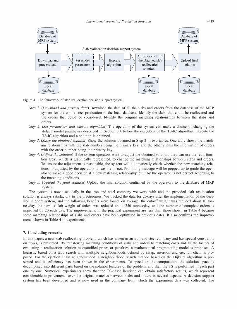
Step 1. (Download and process data) Download the data of all the slabs and orders from the database of the MRPsystem for the whole steel production to the local database. Identify the slabs that could be reallocated andthe orders that could be considered. Identify the original matching relationships between the slabs andorders.

Step 2. (Set parameters and execute algorithm) The operators of the system can make a choice of changing thedefault model parameters described in Section 3.4 before the execution of the TS-IC algorithm. Execute theTS-IC algorithm and a solution is obtained.

Step 3. (Show the obtained solution) Show the solution obtained in Step 2 in two tables. One table shows the match-ing relationships with the slab number being the primary key, and the other shows the information of orderswith the order number being the primary key.

Step 4. (Adjust the solution) If the system operators want to adjust the obtained solution, they can use the ‘edit func-tion area’, which is graphically represented, to change the matching relationships between slabs and orders.To ensure the adjustment is reasonable, the system will automatically check whether the new matching rela-tionship adjusted by the operators is feasible or not. Prompting message will be popped up to guide the oper-ator to make a good decision if a new matching relationship built by the operator is not perfect according tothe matching conditions.

Step 5. (Upload the final solution) Upload the final solution confirmed by the operators to the database of MRPsystem.

The system is now used daily in the iron and steel company we work with and the provided slab reallocationsolution is always satisfactory to the practitioners. We tracked the data for 20 days after the implementation of the deci-sion support system, and the following benefits were found: on average, the cut-off weight was reduced about 10 ton-nes/day, the surplus slab weight of orders was reduced about 250 tonnes/day, and the number of complete orders isimproved by 20 each day. The improvements in the practical experiment are less than those shown in Table 4 becausesome matching relationships of slabs and orders have been optimised in previous dates. It also confirms the improve-ments shown in Table 4 in experiments.

7. Concluding remarks

In this paper, a new slab reallocating problem, which has arisen in an iron and steel company and has special constraintson flows, is presented. By transferring matching conditions of slabs and orders to matching costs and all the factors ofevaluating a reallocation solution to quantified prizes or penalties, a mathematical programming model is proposed. Aheuristic based on a tabu search with multiple neighbourhoods defined by swap, insertion and ejection chain is pro-posed. For the ejection chain neighbourhood, a neighbourhood search method based on the Dijkstra algorithm is pre-sented and its efficiency has been shown in the experiments. To speed up the computation, the solution space isdecomposed into different parts based on the solution features of the problem, and then the TS is performed in each partone by one. Numerical experiments show that the TS-based heuristic can obtain satisfactory results, which representconsiderable improvements over the original matches between slabs and orders in several aspects. A decision supportsystem has been developed and is now used in the company from which the experiment data was collected. The

Database ofMRP system

Download and process data

Execute algorithm

Adjust or confirm the obtained slab

reallocationsolution

Set model parameters

Upload final solution

Database of MRP system

Local database

Local database

Local database

Slab reallocation decision support system

Figure 4. The framework of slab reallocation decision support system.


TS-based heuristic with solution space decomposition and multiple neighbourhoods shows the potential to solve typesof problems such as slab matching problems, slab-design problems and so on.

AcknowledgementsThis work is partly supported by the State Key Program of National Natural Science Foundation of China (grant number 71,032,004),the National Natural Science Foundation of China Grant for Distinguished Young Scholars (grant number 70,728,001) and theNational Natural Science Foundation of China (grant number 60,804,053).

References

Dawande, M., J. Kalagnanam, H. S. Lee, C. Reddy, S. Siegel, and M. Trumbo. 2004. “The Slab-Design Problem in the SteelIndustry.” Interfaces 34 (2): 215–225.

Forrest, J. J. H., J. Kalagnanam, and L. Ladanyi. 2006. “A Column-generation Approach to the Multiple Knapsack Problem withColor Constraints.” INFOMS Journal on Computing 18 (1): 129–136.

Kalagnanam, J. R., M. W. Dawande, M. Trumbo, and H. S. Lee, 1998. “Inventory Matching Problems in the Steel Industry.” IBMResearch Report, Computer Science/Mathematics, RC 21171(94615) May 4, 1998.

Kalagnanam, J. R., M. W. Dawande, M. Trumbo, and H. S. Lee. 2000. “The Surplus Inventory Matching Problem in the ProcessIndustry.” Operations Research 48 (4): 505–516.

Öncan, T. 2007. “A Survey of the Generalized Assignment Problem and Its Applications.” INFOR 45 (3): 123–141.Özbakir, L., A. Baykasoğlu, and P. Tapkan. 2010. “Bees Algorithm for Generalized Assignment Problem.” Applied Mathematics and

Computation 215: 3782–3795.Song, S. H. 2009. “A Nested Column Generation Algorithm to the Meta Slab Allocation Problem in the Steel Making Industry.”

International Journal of Production Research 47 (13): 3625–3638.Woodcock, A. J., and J. M. Wilson. 2010. “A Hybrid Tabu Search/Branch & Bound Approach to Solving the Generalized

Assignment Problem.” European Journal of Operational Research 207: 566–578.Yagiura, M., T. Ibaraki, and F. Glover. 2004. “An Ejection Chain Approach for the Generalized Assignment Problem.” INFORMS

Journal on Computing 16 (2): 133–151.Yagiura, M., T. Ibaraki, and F. Glover. 2006. “A Path Relinking Approach with Ejection Chains for the Generalized Assignment

Problem.” European Journal of Operational Research 169: 548–569.Yeong-Dae, K., B. June-Young, A. Kwee-Yeon, and L. Seung-Kil. 2008. “A Due-date-based Algorithm for Lot-order Assignment in a

Semiconductor Wafer Fabrication Facility.” IEEE Transactions on Semiconductor Manufacturing 21 (2): 209–216.

4420 L. Tang et al.

modelling and a tabu search solution for the slab reallocation

Documents