modeling the nitrogen cycling and plankton productivity in ... · continental shelf regions (depth
TRANSCRIPT

Modeling the nitrogen cycling and plankton productivity in the Black
Sea using a three-dimensional interdisciplinary model
M. Gregoire1
F.N.R.S. Research Associate, Laboratory of Oceanology, Interfaculty Center for Marine Research, University of Liege,Liege, Belgium
K. SoetaertCentre for Estuarine and Marine Ecology, Netherlands Institute of Ecology, Yerseke, Netherlands
N. Nezlin and A. KostianoyP.P. Shirshov Institute of Oceanology, Academy of Sciences of Russia, Moscow, Russia
Received 11 June 2001; revised 7 January 2004; accepted 9 February 2004; published 5 May 2004.
[1] A six-compartment ecosystem model defined by a simple nitrogen cycle is coupledwith a general circulation model in the Black Sea so as to examine the seasonal variabilityof the ecohydrodynamics. Model results show that the annual cycle of the biologicalproductivity of the whole basin is characterized by the presence of a winter–early springbloom. In all the regions this bloom precedes the onset of the seasonal thermoclineand occurs as soon as the vertical winter mixing decreases. Phytoplankton developmentstarts in winter in the central basin, while in coastal areas (except in the river dischargearea) it begins in early spring. In the Danube’s discharge area and along the western coast,where surface waters are almost continuously enriched in nutrient by river inputs, thephytoplankton development is sustained during the whole year at the surface. The seasonalvariability of the northwestern shelf circulation induced by the seasonal variations inthe Danube discharge and the wind stress intensity has been found to have a major impacton the primary production repartition of the area. In the central basin the primaryproduction in the surface layer relies essentially on nutrients being entrained in the upperlayer from below. Simulated phytoplankton concentrations are compared with satelliteand field data. It has been found that the model is able to reproduce the maincharacteristics of the space-time evolution of the Black Sea’s biological productivity butunderestimates the phytoplankton biomass especially in regions extremely rich in nutrientssuch as the Danube discharge area. INDEX TERMS: 4842 Oceanography: Biological and Chemical:
Modeling; 1615 Global Change: Biogeochemical processes (4805); 4815 Oceanography: Biological and
Chemical: Ecosystems, structure and dynamics; 4845 Oceanography: Biological and Chemical: Nutrients and
nutrient cycling; KEYWORDS: mathematical modeling, ecosystem, Black Sea
Citation: Gregoire, M., K. Soetaert, N. Nezlin, and A. Kostianoy (2004), Modeling the nitrogen cycling and plankton productivity in
the Black Sea using a three-dimensional interdisciplinary model, J. Geophys. Res., 109, C05007, doi:10.1029/2001JC001014.
1. Introduction
[2] The Black Sea is known as one of the best examplesof highly stratified marginal seas constituting one of theworld’s largest stable anoxic basin. It is by large a landlocked basin with only restricted exchanges with the Med-iterranean Sea through the Bosphorus Strait (Figure 1).Therefore its overall mass budget and hydrochemical struc-ture critically depend on elements of the hydrologicalbalance. Its hydrographic regime is characterized by low-salinity surface waters of river origin overlying high-salinity
deep waters of Mediterranean origin. As a result, a perma-nent pycnocline (or more precisely a halocline) developswith a depth varying horizontally according to the localhydrodynamics and inhibits the exchanges between thesurface and deep waters.
1.1. Biogeochemical Vertical Structure
[3] The Black Sea possesses a distinct vertical biogeo-chemical structure representing major characteristic featuresof the oxygen deficient pelagic waters of the world’s oceans(Figure 2). The poor ventilation of the deep waters by thevertical mixing and by lateral influxes conjointly with thedegradation of the huge biological production have madethe Black Sea almost completely anoxic with oxygen onlyin the upper 150 m depth (13% of the sea volume) andhydrogen sulfide in the deep waters. The predominant
JOURNAL OF GEOPHYSICAL RESEARCH, VOL. 109, C05007, doi:10.1029/2001JC001014, 2004
1Now at Centre for Estuarine and Marine Ecology, Netherlands Instituteof Ecology, Yerseke, Netherlands.
Copyright 2004 by the American Geophysical Union.0148-0227/04/2001JC001014
C05007 1 of 28

vertical gradients of biogeochemical properties are confinedwithin the strongly stratified upper 100 m layer, in whichthe density changes by about 5 kg/m3 from st � 11.0 kg/m3
at the surface to st � 16.0 kg/m3 at 100 m depth.[4] The water column of the open sea consists of four
biogeochemically distinct layers: (1) the surface layer welloxygenated by the seasonal mixing and by active plank-tonic processes, (2) the oxycline/upper nitracline layercharacterized by a steep decrease of the oxygen concen-tration to about 10mmol O2m
�3 and an increase in the nitrateconcentration to about 6–9mmol Nm�3 due to the oxidationof regenerated ammonium, (3) the transitional layer, the so-called suboxic zone [e.g., Murray et al., 1995], with athickness of about 20–40 m where the oxygen and sulphideconcentrations are low (�<1–5 mmol m�3) with no over-lapping, and (4) the deep anoxic layer of hydrogen sulphideand ammonium pools. In the transitional layer, the oxidation-reduction potential of the water decreases sharply because ofoxygen deficiency and the appearance of hydrogen sulphideat its lower boundary. As a result, this layer contains a rich setof bacterially mediated redox reactions involving oxygen,nitrogen, sulphur, carbon, manganese and iron and so, itslower and upper interfaces are characterized by importantgradients of biological and chemical variables. These reac-
tions control the downward transport of nitrate and theupward transport of ammonium and sulfide near theinterface zone [Oguz et al., 2000]. Also, according tothe chemical model developed by Brewer and Murray[1973], the chemiosynthetic bacterial population at theinterface between oxic and anoxic waters would seem toact as a fairly effective ‘lid’ for the anoxic basin, trappingmuch of the upward flux of carbon dioxide, ammonia andphosphate and returning it to the deep water in particulateform, perhaps forming one of the mechanisms wherebythe Black Sea basin acts as a ‘nutrient trap’. For instance,it was proposed that the upward fluxes of sulfide andammonium may be oxidized by Mn(III, IV) and Fe(III),whereas the downward flux of nitrate may be reduced bydissolved manganese and ammonium [e.g., Murray et al.,1995; Oguz et al., 2000]. The oxidation of ammonium bymanganese into nitrogen gas, which is lost to the atmo-sphere, therefore completely decouples the subpycnoclineammonium source from the near surface nitrogen sourceused for new production. Therefore no new nitrogenwould reach the euphotic zone from the deep watersand so, the nitrogen cycle of the surface layer is inde-pendent of the chemical processes occurring in the deepwaters [e.g., Sorokin, 1983; Yakushev and Neretin, 1997].
Figure 1. Layout and bathymetry of the Black Sea basin (surface = 426,000 km2; volume =534,000 km3). Depth contours are labeled in meters. (Reprinted from Ozsoy and Unluata [1997] withpermission from Elsevier Science.). The northwestern part of the basin is occupied by a wide shelf with amean depth of about 50 m. The middepth at the shelf break is around 150 m. The slope area located at thesouth of the northwestern shelf is defined as the zone with depth between 150 and 2000 m. The bottomtopography used in the model is not the topography shown on this figure but is taken from the UNESCObathymetric map and discretized with the model resolution. The numbers indicate the positions ofdifferent stations chosen according to their particular hydrodynamical and biogeochemical properties toillustrate in more detail the results of the coupled model.
C05007 GREGOIRE ET AL.: MODELING THE BLACK SEA ECOSYSTEM
2 of 28
C05007
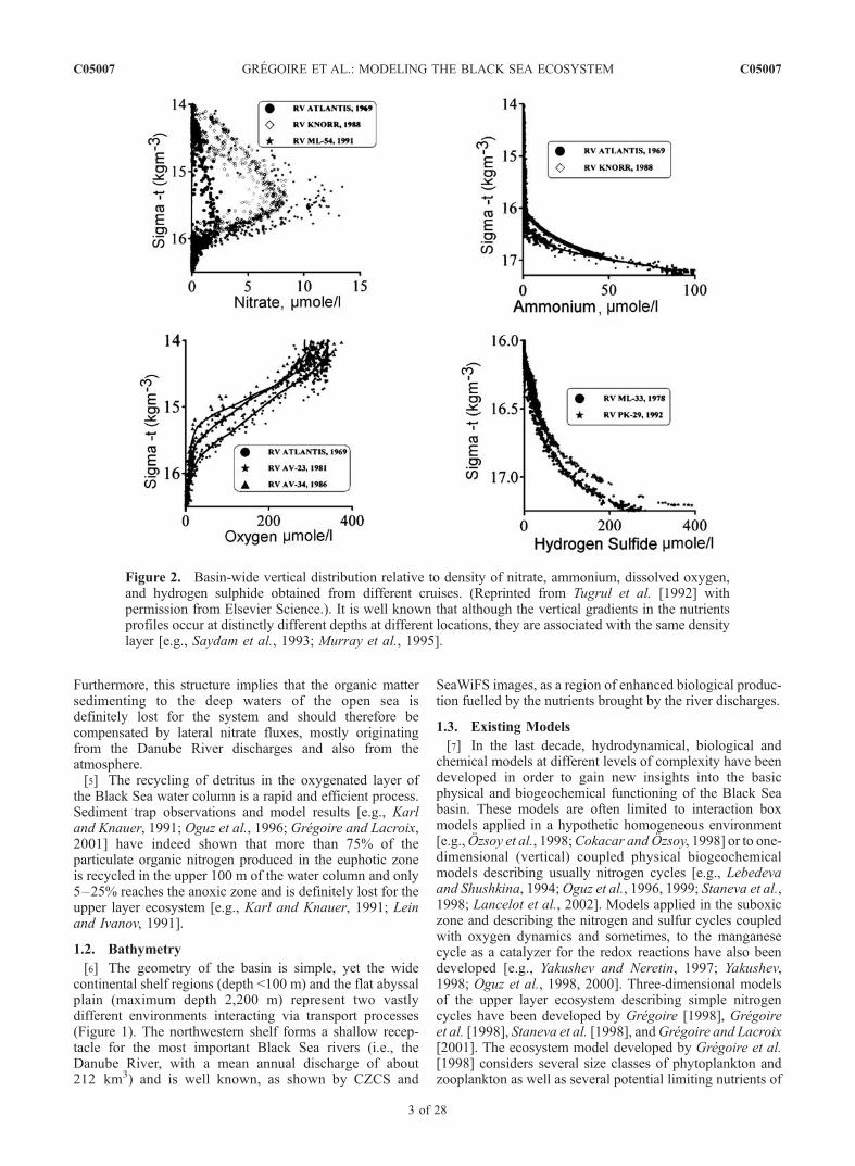
Furthermore, this structure implies that the organic mattersedimenting to the deep waters of the open sea isdefinitely lost for the system and should therefore becompensated by lateral nitrate fluxes, mostly originatingfrom the Danube River discharges and also from theatmosphere.[5] The recycling of detritus in the oxygenated layer of
the Black Sea water column is a rapid and efficient process.Sediment trap observations and model results [e.g., Karland Knauer, 1991; Oguz et al., 1996; Gregoire and Lacroix,2001] have indeed shown that more than 75% of theparticulate organic nitrogen produced in the euphotic zoneis recycled in the upper 100 m of the water column and only5–25% reaches the anoxic zone and is definitely lost for theupper layer ecosystem [e.g., Karl and Knauer, 1991; Leinand Ivanov, 1991].
1.2. Bathymetry
[6] The geometry of the basin is simple, yet the widecontinental shelf regions (depth <100 m) and the flat abyssalplain (maximum depth 2,200 m) represent two vastlydifferent environments interacting via transport processes(Figure 1). The northwestern shelf forms a shallow recep-tacle for the most important Black Sea rivers (i.e., theDanube River, with a mean annual discharge of about212 km3) and is well known, as shown by CZCS and
SeaWiFS images, as a region of enhanced biological produc-tion fuelled by the nutrients brought by the river discharges.
1.3. Existing Models
[7] In the last decade, hydrodynamical, biological andchemical models at different levels of complexity have beendeveloped in order to gain new insights into the basicphysical and biogeochemical functioning of the Black Seabasin. These models are often limited to interaction boxmodels applied in a hypothetic homogeneous environment[e.g., Ozsoy et al., 1998;Cokacar and Ozsoy, 1998] or to one-dimensional (vertical) coupled physical biogeochemicalmodels describing usually nitrogen cycles [e.g., Lebedevaand Shushkina, 1994;Oguz et al., 1996, 1999; Staneva et al.,1998; Lancelot et al., 2002]. Models applied in the suboxiczone and describing the nitrogen and sulfur cycles coupledwith oxygen dynamics and sometimes, to the manganesecycle as a catalyzer for the redox reactions have also beendeveloped [e.g., Yakushev and Neretin, 1997; Yakushev,1998; Oguz et al., 1998, 2000]. Three-dimensional modelsof the upper layer ecosystem describing simple nitrogencycles have been developed by Gregoire [1998], Gregoireet al. [1998], Staneva et al. [1998], andGregoire and Lacroix[2001]. The ecosystem model developed by Gregoire et al.[1998] considers several size classes of phytoplankton andzooplankton as well as several potential limiting nutrients of
Figure 2. Basin-wide vertical distribution relative to density of nitrate, ammonium, dissolved oxygen,and hydrogen sulphide obtained from different cruises. (Reprinted from Tugrul et al. [1992] withpermission from Elsevier Science.). It is well known that although the vertical gradients in the nutrientsprofiles occur at distinctly different depths at different locations, they are associated with the same densitylayer [e.g., Saydam et al., 1993; Murray et al., 1995].
C05007 GREGOIRE ET AL.: MODELING THE BLACK SEA ECOSYSTEM
3 of 28
C05007
the phytoplankton development. This model was used tosimulate the succession of blooms of the different phyto-plankton groups during the first six months of the year (i.e.,the winter-early spring bloom and the end of spring bloomoccurring at depth feeding on regenerated nutrients) and totest the limitation of the phytoplankton development by theavailability of phosphorus and silicate (for diatoms). Thecompetition between the different phytoplankton groups isanalyzed in connection with the variability of the hydrody-namics.Gregoire and Lacroix [2001] refine a classic NAPZDecosystem model (defined by nitrate, ammonium, phyto-plankton, zooplankton and detritus) to describe explicitlythe oxygen dynamics in order to assess the ventilationprocess of the Black Sea’s intermediate layer. Staneva et al.[1998] described and analyzed a few simulations performedwith a NAPZD ecosystem model in connection with the 3Dvariability of the physical environment.[8] In this paper, an ecosystem model has been coupled
with a hydrodynamical model in a 3D frame to understand themacroscale (i.e., timescales of a few weeks to months)ecohydrodynamics over the year. The model has been runfor a few years until it reaches more or les establishedseasonal cycles which, at the scales of our study, do notshow a substantial interannual variability. The results illus-trate a highly complex spatial variability in the phytoplanktonannual cycle imparted by the horizontal and vertical varia-tions of the physical and chemical properties of the watercolumn. Physical structures associated with the verticalstratification (e.g., permanent pycnocline, thermocline), thehorizontal frontal boundaries between river waters and opensea haline waters, and the formation of secondary flows areshown to be of the uppermost importance for the dynamicsand structures of biological populations. The comparison ofthe phytoplankton biomass computed by the model withsatellite-derived estimates and field observations of chloro-phyll concentrations suggests that themodel reproduces quitewell the seasonal plankton productivity cycle in the differentareas of the basin but underestimates the phytoplanktonbiomass in the Danube’s discharge area.[9] This paper is organized as follows. Section 2 describes
the mathematical tool with the assumptions and idealizationsmade. The convergence of the model solution to an estab-lished seasonal cycle is discussed. Section 3 describes theresults of the numerical experiments and their consistencywith observed data. The main findings of the hydrodynamicmodel are summarized, stressing the aspects of the currentand hydrological fields that affect the ecosystem. The sea-sonal variations of the circulation and thermohaline fields aredescribed as well as the space-time evolution of the mixedand mixing layer depths. The seasonal cycle of the phyto-plankton bloom is analyzed emphasizing its regional varia-tions induced by the variations of the local hydrodynamics.The model results are compared with field and satelliteobservations. A discussion on the ability of model resultsto reproduce the observations is given in section 4. Finally,the main conclusions are given in section 5.
2. Mathematical Tool: Description of theThree-Dimensional Model
[10] The three-dimensional model results from the on-linecoupling between a general circulation model and an
ecosystem model. Its equations are formulated in the so-called s coordinate system to follow the bathymetry asclosely as possible. To simulate the general circulation andassociated synoptic structures, the domain is covered with a15 km * 15 km horizontal numerical grid and 25 vertical slayers. The spacing of the vertical layers is adjusted to offera finer resolution in the vicinity of the surface and in theregion of the thermocline (the thickness of the verticallayers is about 5 m in the upper 30 m and 10 m down to100 m). The influence of biogeochemical processes on thehydrodynamics is not taken into account. The velocityvector, the vertical diffusion coefficients and the tempera-ture are computed in the hydrodynamic model and areintroduced at each time step in the ecosystem model.
2.1. Hydrodynamical Model
[11] The GHER general circulation model which has beenused in this study of the Black Sea seasonal ecohydrody-namics is three-dimensional, nonlinear and baroclinic. Ituses a refined turbulent closure scheme and solves themotions of the free surface. It is well known that the verticalturbulent diffusivity coefficients can be expressed in termsof the kinetic energy of the turbulence k and its dissipationrate e. In the GHER model, the equation for e (which, at thegeneral circulation scale contains too many unknown param-eters) is dropped and replaced by an algebraic mixing lengthclosure taking into account the intensity of both the stratifi-cation and the surface wind mixing. The GHER generalcirculation model has been successfully applied to explorethe general circulation of the Bering Sea [e.g., Deleersnijderand Nihoul, 1988], the North Sea [e.g., Delhez, 1996], theMediterranean Sea [e.g., Beckers, 1991] and, more recently,the Black Sea [e.g., Gregoire et al., 1998; Gregoire, 1998;Stanev and Beckers, 1999; Gregoire and Lacroix, 2001,2003].
2.2. Ecosystem Model
[12] The ecosystem model is defined by a simplenitrogen cycle based on the functional role played inthe trophic dynamics by planktonic populations. It isdescribed by 6 aggregated variables: the phytoplanktonand zooplankton biomasses without reference to species,total detritus (lumping together dissolved and particulatedead organic matter), nitrate, ammonium and benthicdetritus. The phytoplankton (j) represents all the primaryproducers. All the heterotrophs with a size rangingbetween 2 mm and 2 mm are described by the zooplank-ton compartment (z). Since the microbial loop of theBlack Sea’s oxygenated waters is particularly efficient[e.g., Sorokin, 1983; Karl and Knauer, 1991], the bacter-ioplankton has been eliminated from the model assumingquasi-equilibrium, prey-predator relationships within themicrobial loop. Nitrogen is the most limiting nutrient ofthe phytoplankton growth to the intense denitrificationprocess occurring in the suboxic layer. In this model,nitrogen is the only limiting nutrient and is divided intoammonium (n1) and nitrate (n2). Nitrite concentrations arenot represented because, on the one hand, in the euphoticlayer data indicate that they are always smaller than theconcentration of other forms of nitrogen [e.g., Codispotiet al., 1991; Basturk et al., 1994] and their contributionto the phytoplankton growth is expected to be small. On
C05007 GREGOIRE ET AL.: MODELING THE BLACK SEA ECOSYSTEM
4 of 28
C05007

the other hand, data reveal that nitrite oxidation rates arealways faster than ammonium oxidation rates (5–10 timesfaster) [Ward and Kilpatrick, 1991]. Besides, followingthe model of Oguz et al. [1999], the introduction ofnitrite production as an intermediate step of the nitrifica-tion process has no distinguishable contribution to theeuphotic zone nitrogen budget. Finally, the dead organicmatter (particulate and dissolved) is described by thedetritus compartment (w), and the sediments are described
by the benthic nitrogen pool bn. A schematic representa-tion of the ecosystem model with all the interaction termswritten on the arrows is given in Figure 3. The evolutionequations of the biogeochemical state variables and themathematical formulation of the biogeochemical interac-tions are described in the Appendix A. The estimation ofbiogeochemical parameters is based on available observa-tions and modeling studies realized in the Black Sea [e.g.,Oguz et al., 1996, 1998; Ozsoy et al., 1998] or in other
Figure 3. Schematic representation of the ecosystem model. All the interaction terms are written onthe arrows and are described in details in Table A1. Fi
j is the nitrogen flux issued from the statevariable i and going to the state variable j. Qy is the production/destruction term of the biogeochemicalstate variable y.
C05007 GREGOIRE ET AL.: MODELING THE BLACK SEA ECOSYSTEM
5 of 28
C05007

similar environments such as the Baltic Sea and the NorthSea. The initial and boundary conditions used to force thehydrodynamical and biogeochemical models are describedin the Appendix B.
2.3. Transient Adjustment
[13] After ten years of integration of the physicalmodel, the amplitude of the seasonal cycle is more orless established in response to the imposed externalforcings and to the internal processes in the system.During the 10-year spin-up, the annual mean verticalstratification does not show substantial trends and remainsclose to the initial data. After this spin-up time, thehydrodynamical model is in balance and the basin inven-tory of water and salt remain constant over the annualcycle [Stanev and Beckers, 1999]. This does not meanthat trends are totally absent but, at the scale of our study(i.e., the seasonal cycle), the small trends, which may bepotentially important for paleoceanography, could notsignificantly affect the results of the model. Using theresults of the tenth year of integration of the physicalmodel, the biological model of the upper layer ecosystemis then integrated to obtain almost repetitive yearly cyclesof the biological variables (this is the case after threeyears of integration).
3. Results
3.1. Hydrodynamics
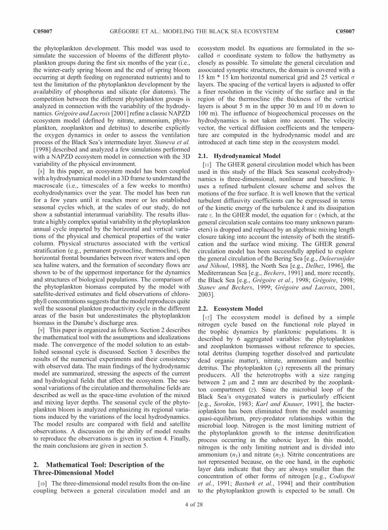
3.1.1. Circulation and Thermohaline Fields[14] A basin-scale, coherent, cyclonic boundary current
that follows approximately the continental slope is the mainfeature of the Black Sea general circulation (Figure 4) [e.g.,Stanev, 1990; Oguz et al., 1992, 1993; Stanev and Beckers,1999]. Referred to as the Rim Current by Oguz et al. [1992,1993], this cyclonic circulation results essentially of thecyclonic wind pattern (positive curl of wind stress) but isalso driven by the large-scale hydrothermodynamic forcing(surface and lateral buoyancy) and is controlled by thetopography [e.g., Stanev, 1990]. As a result, the sea surfaceelevation reaches its maximum value in the coastal zone anddecreases with increasing distance from the coast. Along theAnatolian and Caucasian coasts, where changes in bottomslope and coastline orientation are particularly important,the Rim Current accomplishes large meanders and unstablefeatures are generated on a wide range of space and time-scales [e.g., Blatov et al., 1984; Stanev, 1990; Oguz et al.,1993; Sur et al., 1994].[15] The coastal areas and the central region enclosed by
the Rim Current are occupied by physical structures ofdifferent length scales: a number of cyclonic gyres, inter-acting with the main boundary current and associated withlength scales ranging from a few tenths to a few hundredthsof kilometers, characterizes the circulation of the centralbasin during the whole year with seasonal modifications intheir number, form and position whereas, a series ofsemipermanent anticyclonic eddies exists on the peripherybetween the Rim Current and the undulations of the coast[e.g., Ginzburg et al., 2000, 2001].[16] In spring and summer, the weakening of the wind
stress leads to a decrease of the sea level which tends topromote a cyclonic circulation. Consequently, as shown in
Figure 4 and in agreement with previous studies [Stanev,1990], the intensity of the main current decreases insummer. As a result, the oscillations of the main currentobserved along the Anatolian and Caucasian coasts inten-sify and large meanders with length scales of �100–200 kmare generated. Besides, a weakening of the quasi-permanentcyclonic gyre located in the extreme east of the basin issimulated in agreement with satellite observations whichhave revealed an intensification of the anticyclonic charac-ter of the circulation in the area in summer. In fall, the riverdischarges reach their minimal values and the circulation isdisorganized.[17] The horizontal distribution of the pycnocline depth
shows important gradients resulting from the spatial vari-ability of the hydrodynamics and, in particular, of thevertical circulation. For instance, in the center of thecyclonic gyres, the Ekman pumping generates upwellingsand leads to a rising of the main halocline reducing thedepth of the oxygenated layer to about 90 m. On thecontrary, along the coast, the presence of downwellingsincreases the depth of the oxic layer to about 150 m.Figure 5 compares the horizontal distribution of the depthof the isopycnal st = 16.2 simulated by the model andobtained from the analysis of hydrographic data. Thisdensity corresponds approximately to the depth of appear-ance of H2S [e.g., Vinogradov and Nalbandov, 1990;Saydam et al., 1993].[18] The shallow northwestern shelf constitutes the
coldest part of the Black Sea throughout the year [e.g.,Ozsoy and Unluata, 1997; Ginzburg et al., 2001] andreceives the fresh water inputs of the Danube, Dnestr andDnepr Rivers. This leads to the formation of a stronghaline front which can be observed during the whole yearwith seasonal modifications in its intensity and structureresulting mainly from the pronounced seasonal variabilityof the northwestern shelf circulation (Figure 6). From theend of fall until the middle of spring, the fresh watersfrom the Dnepr and Dnestr are transported southward bythe cyclonic current that occupies the surface northwest-ern shelf waters at this period and mix with the Danubewaters for reaching the Anatolian coast in May. Thestrong haline front confines river waters along the westerncoast and prevents the mixing between the coastal watersand the more saline open seawaters characterized by asalinity of �18–18.2 (Figure 6).[19] One of the most important characteristics of the
seasonal variability of the northwestern shelf circulation onan ecological point of view is the reversal of the surfacecurrent at the middle of spring until the end of fall and thegeneration, at the Danube’s mouth, of an anticyclonic eddywith a length scale of some tens of km (Figure 4). Thisreversal of the flow has also been simulated by Blatov etal. [1984] and Oguz et al. [1995]. It cannot be explainedby the presence of southly winds entraining northward thesurface waters because the climatological monthly meanwind stress used to force the model is from the north fromthe middle of spring until the end of fall except in Juneand July where southly winds prevail. This eddy appearswhen the river discharges intensify and reach their peak.The existence of a cyclonic circulation in the northwesternshelf surface waters from the end of fall until the middleof spring can be explained by the presence of strong
C05007 GREGOIRE ET AL.: MODELING THE BLACK SEA ECOSYSTEM
6 of 28
C05007
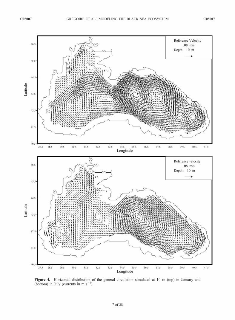
Figure 4. Horizontal distribution of the general circulation simulated at 10 m (top) in January and(bottom) in July (currents in m s�1).
C05007 GREGOIRE ET AL.: MODELING THE BLACK SEA ECOSYSTEM
7 of 28
C05007

northly winds entraining the surface mixing layer (i.e., thezone being actively mixed from the surface) southward. Atthe beginning of spring, when the mixing layer depth isreduced, only the surface waters are entrained southwardby the northly winds. At the middle of spring, the riverdischarges reach their peak and the wind stress is notstrong enough to induce a cyclonic current in the surfacelayer and the circulation becomes anticyclonic. Below themixing layer, the circulation remains anticyclonic duringthe whole year. Besides, some studies have shown that theanticyclonic eddy generated at the Danube’s mouth isbetter represented with a hydrodynamic model using ahigher horizontal resolution [e.g., Gregoire, 1998]. Thisconfirms, in agreement with the previous results of Oguzet al. [1995], that this eddy results more from a nonlineareffect associated to the intrusion of river fresh waters thanfrom a wind effect as suggested by Blatov et al. [1984].
The northeast extension of the haline front in summer hasalso been revealed by salinity measurements (S. Konovalovand L. I. Ivanov, personal communication).3.1.2. Mixed and Mixing Layers[20] The seasonal variations of the mixing layer (i.e.,
the zone being actively mixed from the surface) depth andthe mixed layer depth (i.e., the zone of relatively homo-geneous water formed by the history of mixing) simulatedby the model and obtained from available hydrographicdata [Cokacar and Ozsoy, 1998] are compared in differentareas of the basin which have been chosen according totheir peculiar dynamical and biogeochemical properties(Figure 7).[21] The mixed layer depth corresponds to the zone above
the top of the pycnocline. The peculiar vertical stratificationof the Black Seawaters characterized by the presence of apermanent halocline makes impossible to use criteria based
Figure 5. Horizontal distribution of the depth of the isopycnal st = 16.2 (in meters) (correspondingapproximately to the depth of appearance of H2S) (top) simulated by the model and (bottom) obtainedfrom the analysis of hydrographic data (S. Konovalov, personal communication).
C05007 GREGOIRE ET AL.: MODELING THE BLACK SEA ECOSYSTEM
8 of 28
C05007

only on the temperature gradient to determine the mixedlayer depth. The analyses of mixed layer depths fromhydrographic data made by Cokacar and Ozsoy [1998]suggested that the detection of the mixed layer depth inthe Black Sea required two separate definitions. The firstone, used essentially in summer months (i.e., profileshaving a surface temperature greater than 12�C are consid-ered to belong to summer months), defines the mixed layerdepth as the depth at which a temperature decrease of 1.5�Ctakes place relative to the surface value. The secondcriterion, used in the remaining period, is based on thevertical density gradient, defining the mixed layer depth asthe depth where the density gradient exceeds a value of0.03. The same definitions have been used to determine themixed layer depth in the model.[22] Since the mixing layer depth generally corresponds
to the depth zone in which there is strong turbulence directlydriven by surface forcing, it can be best determined fromvalues of overturning length scales, which are perhaps themost direct measure of active mixing processes [Brainerdand Gregg, 1995]. Indeed, overturning length scales withina convecting layer are dominated by static instabilitiesresulting from cold water in the surface layer and give agood indication of the maximum depth to which theconvection can penetrate. Also, criteria based on the valueof the overturning length scale and on the vertical diffusiv-ity coefficient have been used in this study to identify themixing layer depth.
[23] Figure 7 shows that the mixing layer is obviouslyalways included in the mixed layer and, at the beginning ofspring and in fall, when the level of turbulence is not veryimportant but is high enough to prevent the presence of athermocline, the mixed layer is limited by the upperboundary of the main halocline and can be deeper thanthe mixing layer by more than 60 m. This importantdifference between the mixed and mixing layer depths hasto be taken into account to determine the onset of thephytoplankton winter-early spring bloom as it will bediscussed below. In summer, the mixed and mixing layerdepths are almost the same and coincide approximately withthe upper boundary of the seasonal thermocline.[24] The mixing layer depth varies essentially with the
wind speed and the intensity of the cooling of the seasurface temperatures, deepening where and when the windsand cooling are strong, and shallowing in summer whenwinds are weak. In all the studied areas, the mixing layerdepth reaches its peak in February with important regionalgradients in its distribution. Figure 8 shows, indeed, that it ison the northwestern shelf, outside the river discharge area,and along the western coast, where the cooling and thewinds are the strongest, that the mixing layer is the deepestwith values of about 75 m.[25] Besides, as the upper 90 m of the open seawaters are
more stratified than the coastal areas, mixing layer depthsare shallower in the central basin than along the coast for agiven wind speed; that is, the high stratification of the
Figure 6. Horizontal salinity distribution at 10 m in (a) January, (b) May, (c) July, and (d) October.
C05007 GREGOIRE ET AL.: MODELING THE BLACK SEA ECOSYSTEM
9 of 28
C05007

Figure 7
C05007 GREGOIRE ET AL.: MODELING THE BLACK SEA ECOSYSTEM
10 of 28
C05007

surface layer of the open sea retards mixing layer depthdeepening. For instance, in the center of the cyclonic gyresof the central basin, the winter mixing layer does not extendfurther than 45 m.[26] The summer mixing layer depth does not exceed 5 m
in all the regions. The autumn season is known to becharacterized by weekly storms which are expected toenhance temporarily upward flux of nitrate into the surfacelayer [Oguz et al., 1996]. However, since the model isforced at the air-sea interface by the mean wind stress atmacroscale produced by a monthly mean wind and not, as itshould have been, by the mean wind stress including a quitesignificant component due to nonlinear interactions ofmesoscale winds, small-scale events, such as storms, arenot well represented. This leads to an underestimation of theproduction of turbulent kinetic energy at the surface andtherefore also of the mixing layer depth. On the other hand,at the surface, temperature values are relaxed toward clima-tological monthly mean values and this leads to an overes-timation of surface temperatures. Therefore the verticalmixing by convection is also underestimated. For instance,in November, the surface temperatures of the central basinare relaxed toward about 14�C during the whole month.However, field observations give a surface temperature ofabout 11�C at the mid-November [Oguz et al., 1996].Besides, it should be noted that using a nudging schemefor the temperature to force the model at the surface insteadof the heat fluxes underestimates the vertical penetration ofthe seasonal atmospheric signal. For instance, in spring,
only the first upper 15 m are affected by the seasonalheating of the water column. As a result, in summer, thevertical extension of the thermocline is estimated to about13 m while field observations give a vertical extension ofabout 30 m.[27] The mixed layer depth is limited by the upper
boundary of the main halocline in winter and by the topof the thermocline in summer. In winter, the upward motionof the main halocline in the central basin reduces the mixedlayer depth to about 40–70 m. In particular, in the easternpart of the sea (at longitude 37�E), where the cycloniccurrent is the most intense and the main pycnocline theshallowest, the mixed layer does not extend further than45 m in winter as confirmed by the observations ofOvchinnikov and Popov [1987]. On the other hand, alongthe western coast, south of the Romanian coast, and alongthe Anatolian coast, the downward motion of the mainpycnocline allows the extension of the mixed layer to 70–100 m. On the northwestern shelf, outside the river plume,the water column is almost not stratified. As a result, theRim Current often appears as a boundary between regionsof different mixed layer depths.[28] In the Danube’s discharge area, the intrusion of the
fresh river waters creates a strong vertical stratification andthe mixed layer does not extend further than 30 m. Thisrestriction will create optimal conditions for the develop-ment of the primary production throughout the year.Besides, in agreement with observations, the seasonalthermocline develops earlier (inMarch) and maintains longer
Figure 7. Seasonal variations of the averaged mixed layer depth in the different regions illustrated in Figure 1, (left)obtained from databases (Reprinted from Cokacar and Ozsoy [1998] with permission from Kluwer Academic Publisher;the 95% confidence limits are marked by error bars, solid bars denote values obtained from the recent database (1986–1995), while dashed bars denote values obtained from the Mamayev (1923–1992) database), (right) simulated by the model(in bold). In the model the mixing layer depth has also been represented. The depth of this layer has been defined as thedepth to which a daily average vertical diffusivity coefficient of 10 cm2 s�1 is simulated (in continuous normal line) or adaily average mixing length of 1 m is simulated (in dashed line) (both criteria approximately lead to the same value of themixing layer depth).
Figure 8. Horizontal distribution of the winter mixing layer depth (in meters).
C05007 GREGOIRE ET AL.: MODELING THE BLACK SEA ECOSYSTEM
11 of 28
C05007
(until October/November) in the eastern part of the basin thanin the western and northwestern basin (where the thermoclinestarts in April until August/September) because of the pres-ence of higher atmospheric temperatures and weaker windsin this area at the beginning of spring and fall.[29] The analysis of the seasonal cycle of the mixed and
mixing layer depths confirms that the winter meteorologicalconditions are not severe enough to generate a verticalmixing which is able to erode the main pycnocline whichis therefore permanent and remains throughout the year.
3.2. Ecodynamics
3.2.1. Phytoplankton[30] The seasonal evolution of the surface phytoplankton
spatial pattern simulated by the model is illustrated inFigure 9. Figure 10 shows the SeaWiFS estimates of thesea surface chlorophyll a concentration. Figure 11 comparesthe surface phytoplankton annual cycle obtained frommodel results and observations (satellite and field measure-ments) in different parts of the basin characterized byparticular dynamical conditions. For comparison of phyto-plankton biomass with chlorophyll a observations, one usesa conversion factor of 1 mmol N � 1 mg chl. Thisconversion factor considers an algal carbon to chlorophyllratio of 100 and carbon to nitrogen ratio of 8.5, even thoughthese numbers are subject to seasonal and regional varia-bilities over the Black Sea [e.g., Karl and Knauer, 1991;Oguz et al., 1999]. Both model results and observationsillustrate a highly complex spatial variability of the phyto-plankton annual cycle imparted by the horizontal andvertical variations of the physical and chemical propertiesof the water column.[31] In all the regions, the phytoplankton annual cycle is
characterized by the presence of a winter-early spring bloom.In the Danube’s discharge area and along the western coast,where surface waters are almost continuously enriched inriver nutrient, the phytoplankton development is sustainedduring the whole year at the surface with seasonal modifica-tions in its intensity. Conversely, in the central basin, theprimary production in the surface layer relies essentially onnutrients being entrained in the upper layer from below and awinter-early spring bloom is simulated in agreement withfield observations (Figure 11). Along the Caucasian coast,satellite observations show the presence of high chlorophyllconcentrations throughout the year. This bloom seems to beenhanced by local inputs of nutrients along the coast, and thusit cannot be represented by the model.[32] At the end of spring and in summer, the maximum
development of the phytoplankton is observed at depth,below the thermocline, except at the Danube’s mouth whereit occurs at the surface all over the year. At the beginning offall, the observations reveal the presence of a new bloom inthe surface layer of the central basin. However, this bloom isstrongly underestimated in the model because of the under-estimation of the vertical mixing at this period. The bloomis delayed and only occurs in November–December(Figure 11). Here below, the seasonal evolution of thephytoplankton bloom is described in details on the base ofthe analysis of model results.3.2.1.1. Winter[33] In winter, the enrichment of surface waters in nutrient
depends on the intensity of the vertical mixing and on its
ability to erode substantially the nitracline which coincidesapproximately with the main halocline. Therefore it isnecessary that during a lapse of time, the winter mixingand mixed layers coincide approximately. Figure 7 showsthat this is the case in almost all the regions in February.However, if the vertical mixing is usually beneficial for thebiological production because it deepens the mixing layerand enriches surface waters in nutrient, an intensive mixingmay have a negative effect if it expands the mixing layer sodeep that the phytoplankton spends too much time in lowlight conditions. Indeed, it is usually considered that, whenprimary production relies on nutrients being entrained in theupper layer from below, the most favorable situation mightbe when the critical depth (i.e., the depth at which the integralnet production is zero) equals the depth of the mixing layer[Sverdrup, 1953]. Therefore the cyclonic gyres of the centralbasin are regions particularly favorable to the development ofa winter bloom of the phytoplankton because on the onehand, this is in these regions that the nitracline is theshallowest and, on the other hand, the soft meteorologicalconditions and the shallow pycnocline reduce the mixinglayer depth to about 30–50 m. This bloom reaches its peak inwinter in the eastern cyclonic gyre where the main pycno-cline is the shallowest and in early spring in the western basin(Figure 11). In the Danube’s discharge area, the continualinput of nutrients and the reduction of the mixing layer depthby the presence of a strong vertical stratification allow thedevelopment of phytoplankton in the surface layer through-out the year. All these considerations explain why, inJanuary, the maximum development of phytoplankton issimulated in the surface waters of the eastern main cyclonicgyre of the central basin and also in the Danube’s dischargearea with maximum concentrations of respectively 1.5 and3 mmol N m�3 (Figures 9 and 11). In the coastal areas (alongthe western and Anatolian coasts) and on the northwesternshelf outside the river plume, the phytoplankton concentra-tions do not exceed 1 mmol N m�3 in January because of thelight limitation of its growth. In these regions, model resultsshow that the phytoplankton development intensifies inMarch and reaches concentrations of about 3 mmol N m�3
as soon as the mixing layer depth decreases and becomescomparable to the euphotic layer.[34] It should be noted that everywhere the model shows
that the bloom precedes the onset of the seasonal thermo-cline (Figure 12). This confirms that the formation of athermocline is not always necessary to allow the occurrenceof a phytoplankton bloom as already observed by Oguz etal. [1996]. This emphasizes that the key parameter in theonset of a phytoplankton bloom is more the depth of themixing layer rather than the depth of the mixed layer.[35] In agreement with field observations [Vedernikov
and Demidov, 1993; Mikaelyan, 1995], in the main part ofthe central basin, where the permanent pycnocline moves tothe sea surface and inhibits the penetration at depth of thevertical mixing (Figure 13), the vertical extension of thebloom does not exceed 35–40 m (Figure 14) because ofthe light limitation of the phytoplankton development belowthe pycnocline. Conversely, in coastal areas and on the shelf,phytoplankton populations extend vertically until 70–80 m.3.2.1.2. Spring[36] At the end of April, the horizontal extension of the
high productivity surface waters is reduced (Figure 9).
C05007 GREGOIRE ET AL.: MODELING THE BLACK SEA ECOSYSTEM
12 of 28
C05007

Phytoplankton populations occupy the northwestern shelfand the coastal areas along the western and Anatolian coastsand remain confined close to the coast by the main halinefront. Model results and satellite observations reveal, how-
ever, some large extensions of the bloom toward the opensea along the Anatolian coast where the interactions of themain boundary current with the abrupt modifications of thecoastline orientation and of the topography lead to frontal
Figure 9. Model-simulated sea surface phytoplankton distribution (in mmol N m�3): (a) in January,(b) in March, (c) in May, (d) in June, (e) in August, and (f) in December.
C05007 GREGOIRE ET AL.: MODELING THE BLACK SEA ECOSYSTEM
13 of 28
C05007

instabilities (Figures 9 and 10). In the central basin, thenutrient content of surface waters decreases progressivelyand the phytoplankton populations migrate to greater depthsfeeding on regenerated nutrient. Simulated concentrations
are of about 0.5 mmol N m�3 and are in good agreementwith field and satellite chlorophyll a observations that arebetween 0.2 and 0.5 mg m�3 [Vedernikov and Demidov,1993; Nezlin et al., 1999].
Figure 9. (continued)
C05007 GREGOIRE ET AL.: MODELING THE BLACK SEA ECOSYSTEM
14 of 28
C05007

[37] At the middle of spring, the reversal of the flow onthe northwestern shelf transports the phytoplankton popu-lations in the northeastern part of the shelf. Model results, inagreement with satellite observations (Figures 9 and 10),show the presence of high productivity waters on the wholenorthwestern shelf and along the western and Anatoliancoasts with large intrusions toward the open sea at the shelfbreak. According to Sur et al. [1994], coccolithophoridsdominate the early summer primary production except atthe Danube’s mouth where species rich in chlorophyll adevelop.3.2.1.3. Summer[38] In summer, in a general way, the phytoplankton feeds
mainly on regenerated nutrient and reaches its maximumdevelopment at depth just at the seasonal thermocline,except at the Danube’s mouth where maximum concentra-tions are still observed in the surface layer. For instance, inthe central basin, phytoplankton develops between 15 and
35 m with maximal concentrations of 0.6 mmol N m�3.This value is slightly lower than field observations whichare between 0.75 and 1.2 mmol N m�3 at 40 m [Vedernikovand Demidov, 1993]. Along the Anatolian and westerncoasts, phytoplankton reaches its maximum developmentbetween 15 and 40 m with concentrations between 0.5(along the eastern Anatolian coast) and 1.4 mmol N m�3
(along the western coast).[39] At the end of September, the bloom initiated on the
northwestern shelf in the Danube area continues its propa-gation offshore. This is at this period that the western basinis enriched in the nutrients brought by the rivers on thenorthwestern shelf. However, this enrichment occurs mainlyat depth (about 70–80 m) and therefore does not consider-ably enhance the phytoplankton development. Also, a smallbloom with concentrations of only 0.1–0.2 mmol N m�3
occupies the surface layer of the region at this time(Figure 11). In front of the Caucasian coast, intense upwel-
Figure 10. Seasonal evolution of SeaWiFS estimated surface chlorophyll fields (in mg m�3).
C05007 GREGOIRE ET AL.: MODELING THE BLACK SEA ECOSYSTEM
15 of 28
C05007

Figure 11
C05007 GREGOIRE ET AL.: MODELING THE BLACK SEA ECOSYSTEM
16 of 28
C05007

lings bring to the surface cold nutrient rich waters andenhance the phytoplankton development.3.2.1.4. Autumn[40] The autumn period corresponds to the precondition-
ing and initial cooling phase. The seasonal thermoclineweakens and the deepening of the mixing layer begins bythe end of October. The thermocline collapses almostcompletely on the northwestern shelf while in the centralbasin the simulated mixed layer extends to about 30 m(Figure 7). A secondary bloom is simulated along thewestern coast while in the central basin, the underestimationof the vertical mixing at this period, delays the occurrenceof a new phytoplankton bloom (Figure 11).[41] In November–December, the intensification of the
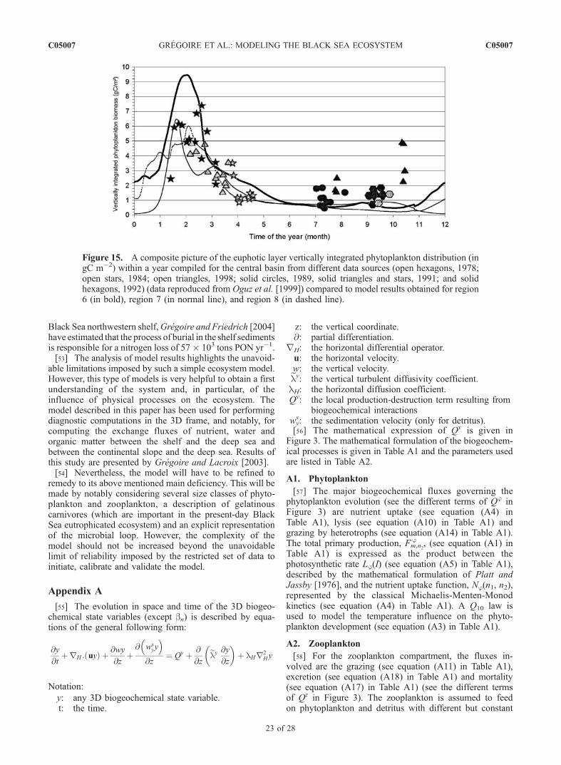
wind stress destroys the seasonal thermocline of the centralbasin. Surface waters are enriched with nutrient entrainedfrom below and a new phytoplankton bloom occurs in thesurface layer of the area (Figure 11).[42] Taking 1 mmol N approximately equivalent to
0.1 gC, the euphotic layer vertically integrated phytoplank-ton biomasses obtained from model results and field obser-vations for the open sea are compared (Figure 15). Theintegrated biomass has its maximum peak in early springwith lower values in the centre of the eastern gyre where themain pycnocline is the shallowest and limits the verticalextension of the phytoplankton bloom to the upper 30–35 m. Values of about 5.5 gC m�2 are simulated in thisregion while values of about 8 gC m�2 are simulated in thewestern basin. These values reflect the typical measuredbiomasses in different parts of the central basin at the sameperiod which are between 5 and 8 gC m�2. In April, asecondary peak of biomass is simulated in the eastern gyreand corresponds to the development of a subsurface bloom.The summer biomass values of about 0.5–0.8 gC m�2 arealso in the range of measured values (0.5–1.5 gC m�2).However, at the beginning of fall, the simulated values arebelow the observations because the model does not simulatethe early autumn bloom in the surface layer.3.2.2. Nitrate[43] In the deep basin where waters below 100–150 m
are anoxic, the vertical nitrate profile is characterized bythe presence of a nitracline throughout the year (Figures 2and 12). Indeed, the oxidation of the ammonium producedin the regeneration of detritus leads to the formation of anitrate peak and below, nitrate decreases with depth likelybecause of heterotrophic denitrification. Therefore thisnitrate maximum corresponds to the transition betweenthe nitrification and denitrification processes in the watercolumn. Its position varies horizontally according to thelocal physical and biogeochemical properties of the watercolumn. For instance, in the central basin, the maximum isobserved at 60–80 m while, along the Anatolian coast,maximum concentrations are reached at about 100 m(Figure 12).
[44] In winter, the vertical mixing erodes partially thenitracline and the nitrate concentration in the mixing layerreaches about 2 mmol N m�3 in the central basin, 3.7 mmolN m�3 and 1.4 mmol N m�3 along respectively the westernand eastern Anatolian coast, 5 mmol N m�3 along thewestern coast and 15 mmol N m�3 in the Danube’sdischarge area. In summer, nitrate is below detection limitin the euphotic zone of the central basin and increases belowthis depth region because of the oxidation of regeneratedammonium. Conversely, the surface waters of the north-western shelf and along the western coast are continuouslyfed in the nutrient brought by the rivers on the northwesternshelf. However, this is only at the end of the year that therich nutrient river waters reach the central basin and enrichthe region in nutrient (in September, for the western basinand in December, for the eastern basin).3.2.3. Ammonium[45] During the whole year, the ammonium content is
minimal in the surface layer with a typical concentrationthat does not exceed 0.1–0.2 mmol N m�3 (Figure 12). Atthe base of the euphotic layer, the ammonium concentrationincreases after the winter-early spring bloom and reaches amaximum of about 0.5 mmol N m�3 because of therecycling of detritus. In summer, this regenerated am-monium is oxidized into nitrate. In the upper part of theanoxic layer, where the nitrification process ceases because ofthe lack of oxygen, the ammonium concentration increases.3.2.4. Zooplankton[46] In the central basin, the zooplankton reaches its peak
of development in April, about one month after the winter-early spring bloom. The use of a threshold feeding concen-tration in the mathematical expression of the zooplanktongrazing rate leads to the absence of zooplankton develop-ment when the prey biomass is below the threshold feedingconcentration. This explains why, in the central basin, thezooplankton reaches very small concentrations in summer.While along the western coast and on the northwesternshelf, where the phytoplankton is abundant and wherewaters are enriched in detritus by river discharges, thezooplankton prey concentration is sufficiently high to sus-tain a significant growth of the zooplankton from the end ofspring until the end of fall, with one or two peaks ofdevelopment following phytoplankton blooms. Therefore,in these regions the zooplankton maintains a strongcontrol on the phytoplankton development and preventsits explosion.3.2.5. Detritus[47] The detritus seasonal cycle follows the living organic
matter cycle (phytoplankton and zooplankton) and is alsoinfluenced by river discharges. The concentration of detritusis maximum after the winter-spring bloom with valuesvarying horizontally between 0.3 (in the open sea) and0.8 mmol N m�3 (on the shelf and along the western coast).This is also at this period that the sedimentation velocity is
Figure 11. Seasonal variations of the phytoplankton surface concentration simulated by the model (in mmol N m�3) andof the surface chlorophyll a concentration (mg m�3) obtained from field and satellite observations (top) in the western opensea, (middle) in the eastern open sea, and (bottom) in the eastern Anatolian coast. Solid lines demonstrate the model results,dashed lines demonstrate the range of variations of CZCS-measured plant pigment concentration (25 and 75 percentiles)[Nezlin et al., 1999], and lozenges demonstrate the published results of field observations [e.g., Vedernikov and Demidov,1993].
C05007 GREGOIRE ET AL.: MODELING THE BLACK SEA ECOSYSTEM
17 of 28
C05007

maximum and detritus accumulates below the surface wateruntil about 150 m. Concentrations gradually decrease at theend of spring because of remineralization into ammonium.In summer, detritus accumulates below the seasonal ther-mocline to 100 m along the western coast, and 60–70 m inthe open sea, with concentrations of about 0.1–0.2 mmol Nm�3 in July/August. Almost all the organic matter producedin the euphotic layer is remineralized in the oxygenatedlayer. The model estimates to about 40 � 103 tons theannual loss of particulate organic nitrogen toward theanoxic waters.
4. Discussion and Conclusions
[48] A 3D coupled biogeochemical-hydrodynamicalmodel has been used to analyze and explain the spatialand temporal variability of the seasonal cycle of thebiological productivity in connection with the variabilityof the hydrodynamical and chemical properties of the watercolumn. The hydrodynamical model is able to reproduce themain features of the Black Sea hydrodynamics. In particu-lar, the cyclonic circulation and interior upwellings inducedby the wind field are simulated as well as the frontal systemon the northwestern shelf. The biogeochemical model isdefined by a simple nitrogen cycle based on the functionalrole played in the trophic dynamics by planktonic popula-tions. It is described by six compartments: the phytoplank-ton and zooplankton biomasses, nitrate, ammonium, pelagicand benthic detritus. After 3 years of spin-up run, theamplitude of the simulated seasonal cycle is more or lessestablished and the results of an additional annual simula-tion are compared with satellite images and field observa-tions collected in the area. The biogeochemical resultsillustrate a highly complex spatial variability in the phyto-plankton annual cycle imparted by the horizontal andvertical variations of the physical and chemical propertiesof the water column. The annual cycle of the biologicalproductivity of the whole basin is characterized by thepresence of a winter-early spring bloom. In all the regions,this bloom precedes the onset of the seasonal thermocline. Itoccurs as soon as the mixing layer depth reduces andbecomes comparable or shallower than the euphotic layerdepth. In the Danube’s discharge area and along the westerncoast, where surface waters are almost continuouslyenriched in nutrient by river inputs, the phytoplanktondevelopment is sustained during the whole year at thesurface with seasonal modifications in its intensity. Theseasonal variability of the northwestern shelf circulationinduced by the seasonal variations in the Danube dischargeand the wind stress intensity has been found to have a majorimpact on the primary production repartition of the area.[49] At the end of spring and in summer, the maximum
development of the phytoplankton is observed at depthbelow the thermocline almost everywhere, except at theDanube’s mouth where it occurs at the surface all over theyear. The early autumn bloom revealed by field and satelliteobservations in the central basin is postponed to the end of
fall in the model. This delay is essentially caused by theunderestimation, in the model, of the vertical mixing at thebeginning of fall because this period is characterized byweekly storms which are expected to enhance temporarilythe upward flux of nitrate into the surface layer [Oguz et al.,1996] but are not adequately represented in the model.[50] The qualitative comparison of model results with
SeaWiFS satellite data shows that the model reproducesreasonably well the space-time evolution of the phytoplank-ton distribution. On a quantitative point of view, it seems,however, that in the Danube’s discharge area, the bloomintensity is underestimated by the model. Indeed, thesimulated concentrations are of about 1 mmol N m�3 andare far below field and satellite observations which givevalues for the chlorophyll a concentration of about 4 mgm�3 and even more. Nevertheless, it should be noted that,according to Longhurst et al. [1995], satellite data mayoverestimate, chlorophyll concentrations of marginal seasand coastal areas, especially because of the presence of highconcentrations of yellow substances in suspension. In theDanube’s discharge area and along the western coast, wherenutrients are abundant in the surface layer throughout theyear allowing the growth of phytoplankton at saturationconditions, model results have shown that the most limitingfactor of the phytoplankton development is the grazingpressure (except in winter when, in coastal areas, the lightavailability is the most limiting factor). In these regions, thephytoplankton reaches its peak of development in Marchwith concentrations of 4.5 mmol N m�3 on the northwesternshelf and 3.5 mmol N m�3 along the western coast.However, as soon as the phytoplankton biomass reaches athreshold value, its development is rapidly controlled by thezooplankton that maintains a strong pressure throughout theyear and prevents the explosion of the phytoplankton. Also,although the nutrient content of surface waters in theseregions is extremely high and could sustain huge blooms,the phytoplankton biomass does not exceed 1 mmol N m�3.This particularity seems to be typical of simple ecosystemmodels considering only one phytoplankton compartmentand one zooplankton compartment. Similar conclusionshave been found earlier by Sarmiento et al. [1993] in theirNorth Atlantic model and by Oguz et al. [1999] in theirBlack Sea model. As a result, the totality of the hugeamount of nitrate discharged every year by the rivers onthe shelf cannot be consumed and does not participate to theupper layer nitrogen cycling.[51] Some sensitivity studies of the model solution to the
value of biogeochemical parameters have shown that thesimulation of more intense phytoplankton blooms with sucha simple model requires an unrealistic 10-fold decrease ofthe zooplankton grazing rate. Conversely, an unrealistic10-fold increase of the phytoplankton maximum growthrate does not lead to an increase of the bloom intensity butto an increase of the zooplankton biomass stressing thestrong control played by the zooplankton on the phyto-plankton development. On the other hand, Armstrong[1994] pointed out that multiple prepredator models can
Figure 12. Seasonal variations of the vertical profiles of the biogeochemical state variables and of the temperature field inthree typical areas of the basin characterized by peculiar hydrodynamical and biogeochemical properties: (a) the centralbasin (region 6), (b) the western coast (region 3), and (c) the Anatolian coast (region 4).
C05007 GREGOIRE ET AL.: MODELING THE BLACK SEA ECOSYSTEM
18 of 28
C05007
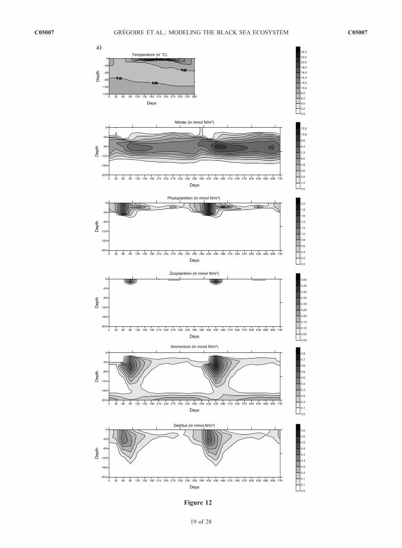
Figure 12
C05007 GREGOIRE ET AL.: MODELING THE BLACK SEA ECOSYSTEM
19 of 28
C05007
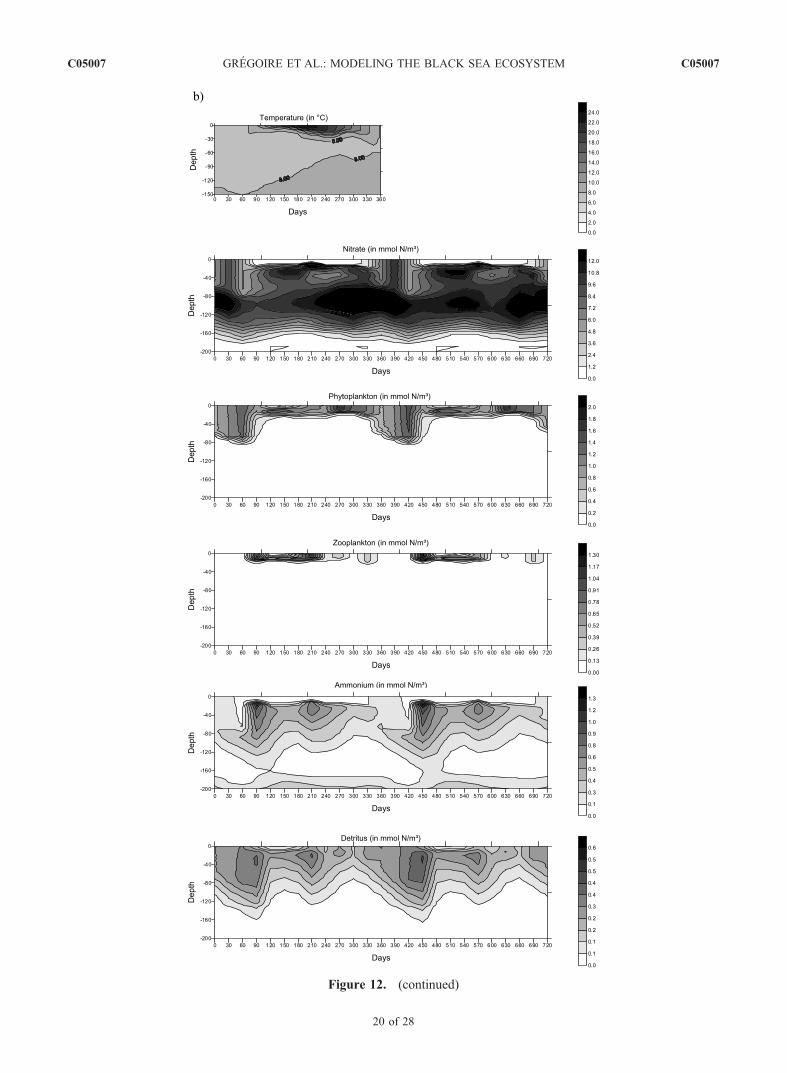
Figure 12. (continued)
C05007 GREGOIRE ET AL.: MODELING THE BLACK SEA ECOSYSTEM
20 of 28
C05007
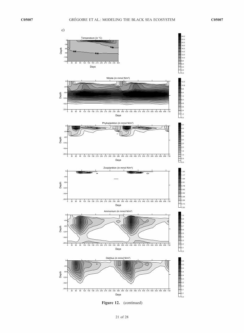
Figure 12. (continued)
C05007 GREGOIRE ET AL.: MODELING THE BLACK SEA ECOSYSTEM
21 of 28
C05007

alleviate the limitations imposed by 1P1Z model and, as inthe North Atlantic case, may generate increased chlorophyllconcentrations comparable with observations [Oguz et al.,1999].[52] Model results in agreement with previous studies
[e.g., Yakushev and Neretin, 1997; Konovalov et al., 2000]have shown that the denitrification process occurring in the
suboxic layer constitutes the main process of nitrogenelimination in the Black Sea providing its ability to resistto the dramatic eutrophication process. 67% (i.e., 4.5 �105 tons N yr�1) of the total annual load of nitrogen broughtinto the Black Sea shelf by the rivers is irreversibly lost bydenitrification. For comparison, on the base of in situ mea-surements performed during the EROS-21 expeditions on the
Figure 13. Horizontal distribution of the turbulent kinetic energy at 40 m in February (in 10�3 m2 s�2).
Figure 14. Horizontal distribution of the phytoplankton field at 40 m in February (in mmol N m�3).
C05007 GREGOIRE ET AL.: MODELING THE BLACK SEA ECOSYSTEM
22 of 28
C05007
Black Sea northwestern shelf,Gregoire and Friedrich [2004]have estimated that the process of burial in the shelf sedimentsis responsible for a nitrogen loss of 57� 103 tons PON yr�1.[53] The analysis of model results highlights the unavoid-
able limitations imposed by such a simple ecosystem model.However, this type of models is very helpful to obtain a firstunderstanding of the system and, in particular, of theinfluence of physical processes on the ecosystem. Themodel described in this paper has been used for performingdiagnostic computations in the 3D frame, and notably, forcomputing the exchange fluxes of nutrient, water andorganic matter between the shelf and the deep sea andbetween the continental slope and the deep sea. Results ofthis study are presented by Gregoire and Lacroix [2003].[54] Nevertheless, the model will have to be refined to
remedy to its above mentioned main deficiency. This will bemade by notably considering several size classes of phyto-plankton and zooplankton, a description of gelatinouscarnivores (which are important in the present-day BlackSea eutrophicated ecosystem) and an explicit representationof the microbial loop. However, the complexity of themodel should not be increased beyond the unavoidablelimit of reliability imposed by the restricted set of data toinitiate, calibrate and validate the model.
Appendix A
[55] The evolution in space and time of the 3D biogeo-chemical state variables (except bn) is described by equa-tions of the general following form:
@y
@tþrH : uyð Þ þ @wy
@zþ@ ws
yy� �@z
¼ Qy þ @
@zely @y
@z
� �þ lHr2
Hy
Notation:
y: any 3D biogeochemical state variable.t: the time.
z: the vertical coordinate.@: partial differentiation.
rH: the horizontal differential operator.u: the horizontal velocity.w: the vertical velocity.ely: the vertical turbulent diffusivity coefficient.lH: the horizontal diffusion coefficient.Qy: the local production-destruction term resulting from
biogeochemical interactionswys: the sedimentation velocity (only for detritus).[56] The mathematical expression of Qy is given in
Figure 3. The mathematical formulation of the biogeochem-ical processes is given in Table A1 and the parameters usedare listed in Table A2.
A1. Phytoplankton
[57] The major biogeochemical fluxes governing thephytoplankton evolution (see the different terms of Qj inFigure 3) are nutrient uptake (see equation (A4) inTable A1), lysis (see equation (A10) in Table A1) andgrazing by heterotrophs (see equation (A14) in Table A1).The total primary production, Fm,n2
j , (see equation (A1) inTable A1) is expressed as the product between thephotosynthetic rate Lj(I) (see equation (A5) in Table A1),described by the mathematical formulation of Platt andJassby [1976], and the nutrient uptake function, Nj(n1, n2),represented by the classical Michaelis-Menten-Monodkinetics (see equation (A4) in Table A1). A Q10 law isused to model the temperature influence on the phyto-plankton development (see equation (A3) in Table A1).
A2. Zooplankton
[58] For the zooplankton compartment, the fluxes in-volved are the grazing (see equation (A11) in Table A1),excretion (see equation (A18) in Table A1) and mortality(see equation (A17) in Table A1) (see the different termsof Qz in Figure 3). The zooplankton is assumed to feedon phytoplankton and detritus with different but constant
Figure 15. A composite picture of the euphotic layer vertically integrated phytoplankton distribution (ingC m�2) within a year compiled for the central basin from different data sources (open hexagons, 1978;open stars, 1984; open triangles, 1998; solid circles, 1989, solid triangles and stars, 1991; and solidhexagons, 1992) (data reproduced from Oguz et al. [1999]) compared to model results obtained for region6 (in bold), region 7 (in normal line), and region 8 (in dashed line).
C05007 GREGOIRE ET AL.: MODELING THE BLACK SEA ECOSYSTEM
23 of 28
C05007

capture efficiencies (see equation (A13) in Table A1). Theingestion rate, Fj;w
z , as a function of the food concentrationis assumed to follow a Michaelis-Menten type relationshipconsidering that when the prey concentration is under agiven threshold the zooplankton ceases its feeding activity[e.g., Mullin, 1963; Andersen and Nival, 1988].
A3. Pelagic Detritus
[59] The zooplankton fecal pellets (see equation (A16) inTable A1), constituting the unassimilated part of theingested food, as well as the phytoplankton and zooplank-ton lysis (see equations (A10) and (A17) in Table A1) arethe source of detritus. Detritus are recycled in the watercolumn as a result of ingestion by zooplankton (see equa-tion (A15) in Table A1) and remineralization into ammo-nium (see equation (A19) in Table A1) (see the different
terms of Qw in Figure 3). They are also submitted tosedimentation. The detritus migration velocity, ww
s , isexpressed as a function of the detritus concentration to takeinto account that at high concentrations, detritus can formaggregate and this aggregation speeds up the sedimentation[e.g., Totterdell et al., 1993; Oguz et al., 1998].
A4. Benthic Detritus
[60] Benthic detritus are formed by the sedimentingparticulate organic nitrogen which is deposited on thebottom (see the different terms of Qbn in Figure 3). Theyare recycled via benthic remineralization according to afirst-order law proposed by Billen and Lancelot [1988] (seeequations (B1) and (B2) in Appendix B). As a result,ammonium is injected from the benthic compartment intothe bottom layer of the water column.
Table A1. Mathematical Formulation of the Biogeochemical Processes
Symbol Mathematical Expression of the Biological Processes Equation Number
Fjn1 ;n2
Flux of nitrogen consumed by phytoplanktonFjn1 ;n2
¼ mj I ;T ; n1; n2ð Þj (A1)mj I ;T ; n1; n2ð Þ ¼ mmj
T ¼ 20Cð ÞJj Tð ÞNj n1; n2ð ÞLj Ið Þ (A2)
Jj Tð Þ ¼ QT�2010
10 (A3)Nj n1; n2ð Þ ¼ n1
cn1þn1þ n2
cn2þn2exp �yn1ð Þ (A4)
Lj Ið Þ ¼ tanhaI zð Þ
mmj T¼20Cð ÞJj Tð Þ
h i(A5)
I zð Þ ¼ I z ¼ 0ð Þ exp �R z
0k zð Þdz
(A6)
k ¼ kw þ kjj (A7)Fn1
j Flux of ammonium consumed by phytoplankton
Fjn1¼ mmj
T ¼ 20Cð Þqj Tð ÞLj Ið Þ n1
cn1 þ n1j (A8)
Fn2
j Flux of nitrate consumed by phytoplankton
Fjn2¼ mmj
T ¼ 20Cð ÞJj Tð ÞLj Ið Þ n2
cn2 þ n2exp �yn1ð Þj (A9)
Fjw Flux of phytoplankton mortality
Fwj ¼ dwjj (A10)
Fj,wz Flux of zooplankton ingestion
Fzj;w ¼ dzj;w bzð Þz ¼ dzj;w
� �max
xczþx
U xð Þz (A11)
x ¼ bz j;wð Þ � b0z (A12)bz j;wð Þ ¼ ezjjþ ezww (A13)where U(x) is the Heaviside function
Fjz Flux of phytoplankton ingestion by zooplankton
F zj ¼ d zj bz;jð Þz ¼ dzj;w bzð Þ
bz j;wð Þ ezjjz (A14)
Fwz Flux of detritus ingestion by zooplankton
Fzw ¼ dzw bz;wð Þz ¼ dzj;w bzð Þ
bz j;wð Þ ezwwz (A15)
pFzw Flux of zooplankton egestion
pFwz ¼ 1� azð ÞFz
j;w (A16)(1 � p)Fz
w Flux of zooplankton mortality1� pð ÞFw
z ¼ mzz (A17)Fn1z Flux of zooplankton excretion
Fn1z ¼ dn1z z (A18)
Fn1w Flux of detritus remineralisation
Fn1w ¼ dn1w w (A19)
Fn2n1
Flux of nitrificationFn2n1
¼ dn2n1 fn sð Þn1 (A20)
fn sð Þ ¼ f 0n U s1 � sð Þ þ gn sð ÞRn þ gn sð ÞU s� s1ð ÞU s2 � sð Þ (A21)
where U(x) is the Heaviside functionFN2n2
Flux of denitrificationFN2n2
¼ dN2
n2fd sð Þn2 (A22)
fd sð Þ ¼ Rd
Rdþgd sð ÞU s� s2ð Þ (A23)
C05007 GREGOIRE ET AL.: MODELING THE BLACK SEA ECOSYSTEM
24 of 28
C05007

A5. Ammonium
[61] The excretion of zooplankton (see equation (A18)in Table A1) as well as the remineralization of detritus(see equation (A19) in Table A1) constitute the ammo-nium sources. The consumption of ammonium resultsfrom its uptake by phytoplankton (see equation (A8) inTable A1) and its oxidation into nitrate in the nitrificationprocess occurring in aerobic waters (see equation (A20)in Table A1) (see the different terms of Qn1 in Figure 3).The depth distribution of nitrification is tied to the supplyof ammonium from decomposition of organic matter andis restricted to very low light or aphotic regions becauseof light inhibition of nitrifying bacteria. Indeed, accordingto several authors [e.g., Olson, 1981; Wada and Hattori,1991], nitrification is photo-inhibited and limited todepths of 1–0.1% light penetration for the oxidation ofammonium into nitrite, depths of less than 0.1% lightpenetration for the oxidation of nitrite into nitrate. Oneshould expect then that the nitrification process affectsthe lower layers of the euphotic zone until the lower
boundary of the oxycline below which the oxygencontent of the water becomes insufficient to allow theoxidation of ammonium. The nitrification is particularlyactive at the base of the euphotic layer where theammonium produced by the regeneration of the deadorganic matter accumulates.[62] In this paper, the nitrification process is not light-
dependent because the ammonium produced by the regen-eration of detritus accumulates mainly below the euphoticzone. It has been short-circuited and modeled as a directconversion of ammonium into nitrate without the interme-diate level of nitrite formation. In the Black Sea, itstimescale ranges between 17 and 60 days [Ward andKilpatrick, 1991], and thus this process belongs to thespectral window of the modeled processes. In the centralbasin, it plays a key role by preventing a progressiveexhaustion of the nitrate consumed by the primary pro-ducers and an accumulation of the ammonium produced byheterotrophic excretion and organic matter regeneration. Onthe shelf, the nitrification process amplifies the input of
Table A2. Signification, Values and Units of the Parameters Used in the Formulation of the Biological
Interaction Terms
Parameters Signification Units Value
Phytoplanktonmmj
(T = 20�C) growth rate at 20�C d�1 3Q10 Q10 factor - 1.88cn1 half-saturation constant for ammonium uptake mmol N m�3 0.2cn2 half-saturation constant for nitrate uptake mmol N m�3 0.5y constant of inhibition of nitrate uptake
by the presence of ammonium(mmol N m�3)�1 1.46
a photosynthetic efficiency (Wm�2)�1d�1 0.015kw pure water diffusive attenuation coefficient m�1 0.08kj phytoplankton attenuation coefficient m�1(mmol N m�3)�1 0.07djw mortality rate d�1 0.05
Zooplankton(dj,w
z )max maximum grazing rate d�1 0.9az assimilation efficiency - 0.75cz Half-saturation constant for ingestion mmol N m�3 0.5b0z threshold concentration mmol N m�3 0.6ezj capture efficiency of phytoplankton - 0.7ezw capture efficiency of detritus - 0.5
dn1z excretion rate d�1 0.1
mz mortality rate d�1 0.05
Nitrification and Denitrificationdn2n1 maximum nitrification rate d�1 0.1Rn half-saturation constant for the limitation function
of the nitrification process by the availability of oxygenmmol O2 m
�3 10
fn0 value of the limitation function of the nitrification
process by the availability of oxygen in surface waters- 0.87
s1 density of the oxycline upper boundary kg m�3 14.8s2 density above which the nitrification process ceases
because of oxygen deficiency and the denitrificationprocess starts to occur
kg m�3 15.6
dN2n2
maximum denitrification rate d�1 0.015Rd constant used in the inhibition function of the
denitrification rate by the presence of oxygenmmol O2 m
�3 2.5
Detritusdn1w remineralization rate d�1 0.07(ws
w)max maximum detrital singing velocity m d�1 8cw half-saturation constant used in the expression
of the detritus sinking ratemmol N m�3 0.2
Sedimentsksed benthic detritus remineralization rate d�1 0.03
C05007 GREGOIRE ET AL.: MODELING THE BLACK SEA ECOSYSTEM
25 of 28
C05007

nitrate by the rivers by oxidizing the ammonium formed bythe remineralization of the huge amount of dissolvedorganic nitrogen discharged by the Danube.
A6. Nitrate
[63] The nitrification process constitutes the only internalsource of nitrate associated to biogeochemical processes (seeequation (A20) in Table A1). The consumption of nitrateresults from its uptake by phytoplankton (see equation (A9)in Table A1) and its reduction into nitrogen gas (i.e., thedenitrification) (see equation (A22) in Table A1) (see thedifferent terms of Qn2 in Figure 3). Heterotrophic denitrifi-cation occurring in waters deficient in oxygen constitutes themain process leading to nitrate exhaustion in the transitionallayer. Nitrate reduction results in the formation of nitrite and,in the final stage, of nitrogen gas that can escape to theatmosphere. Thus this process represents a loss of nitrogenfor the Black Sea. Ward and Kilpatrick [1991] measured thenitrate reduction rate by 15N tracer addition during the 1988Knorr expedition. In the suboxic zone characterized bynitrate concentrations between 2 and 8 mmol N m�3, thisrate ranged from 0.6 � 10�6 to 60 � 10�6 mmol N m�3 d�1
[Oguz et al., 2000]. If all the nitrate reduction can beattributed to heterotrophic denitrification, then the denitrifi-cation rate can roughly be estimated to 0.001–0.002 d�1.This value is thus at least one order of magnitude lower thanthe typical rate of the biogeochemical processes modeled inthis paper. However, to reach a steady state solution in themodel, the denitrification process has absolutely to be takeninto account to prevent the progressive accumulation of thehuge nitrate stock discharged by the rivers.[64] According to Murray et al. [1995] and Oguz et al.
[1998], nitrate is also used to oxidize NH4 and H2S at thelower part of the transitional layer. These processes lead tothe formation of nitrogen gas and are particularly importantbecause they prevent the NH4 and H2S diffusing from theanoxic waters to reach the euphotic layer. However, theircontribution to the consumption of the nitrate of thetransitional layer is negligible comparing to the denitrifica-tion process [e.g., Yakushev and Neretin, 1997], and thusthey have not been represented in this model.[65] The occurrence of the nitrification/denitrification
process is conditioned by the presence/absence of oxygenin the water column. According to Yakushev and Neretin[1997] and Oguz et al. [1998], the nitrification and denitri-fication rates can be expressed by the following mathemat-ical expression:
Fba ¼ dbaf O2ð Þa
where, dab, is the maximum nitrification/denitrification rate,
f(O2), is an nondimensional function of the dissolvedoxygen concentration modeling the positive/inhibitinginfluence of oxygen on nitrification/denitrification, a andb, are respectively n1, n2 in the nitrification process and n2,N2 in the denitrification process.[66] Figure 2 shows that the vertical oxygen profile on a
density scale reveals a rather simple structure throughout thebasin without possessing any seasonal variability [e.g.,Buesseler et al., 1994; Saydam et al., 1993]. This makespossible to use it diagnostically in the biogeochemicalmodel. This characteristic has been confirmed by themodeling studies of Oguz et al. [1998], and therefore the
nitrification/denitrification process can be represented by anequation of the following type:
Fba ¼ dba g sð Þa
where, g(s), is an adimensional function of the density.Equations (A20)–(A21) and (A22)–(A23) in Table A1 givethe mathematical expression of the nitrification anddenitrification processes, respectively, used in this paper.
Appendix B
B1. Initial Conditions
[67] The hydrodynamic model is initialized with horizon-tally homogeneous temperature and salinity fields presentinga vertical stratification typical of the mean climatologicalBlack Sea state. The most important characteristics of thevertical stratification are the sharp halocline from the seasurface down to 200 m and the cold intermediate layer (CIL),analogous to the 18�C water layer in the Atlantic Ocean[Stanev and Beckers, 1999]. The initial vertical profiles ofinorganic nutrients are computed as a function of the densityrather than depth so as to exclude variability resulting fromdynamical effects. Spatial and temporal mean vertical pro-files on a density scale reconstructed from in situ datacollected during the 1988 Knorr and 1991 Bilim researchcruises throughout the Black Sea are used (profiles takenfrom Tugrul et al. [1992] and Saydam et al. [1993]). TheNH4 concentration in the deep waters is set initially to zerobecause, on the one hand, this ammonium does not take partin the nitrogen cycle of the oxygenated layer [e.g., Brewerand Murray, 1973; Murray et al., 1995; Yakushev andNeretin, 1997; Oguz et al., 2000] and, on the other hand,the model does not represent some important chemicalreactions involving, notably, the manganese and iron cycleswhich prevent the ammonium of the deep basin reaching theeuphotic layer. For the organic matter (living and dead),initial constant values are imposed.
B2. Boundary Conditions
[68] The hydrodynamic model is forced by monthly meanclimatological forcing functions. In particular, this includesthe large-scale free surface gradients along the BosphorusStrait, the wind stress at the air-sea interface and the outflowof the Danube, the Dnepr and the Dnestr Rivers on thenorthwestern shelf. Since the contribution to the water budgetof the basin of the Bulgarian and Turkish rivers discharge issmall, their water inputs are regularly distributed in the abovementioned model rivers. The wind stress curl is cyclonicduring the whole year with a maximum in January and aminimum in April–May. Contrary to the wind stress curl,which has a single maximum, the wind stress magnitudereaches two maxima (in winter and summer) and two minima(in spring and fall) [Staneva and Stanev, 1999]. The windstress data are based on ship observations. Temperature andsalinity values are relaxed toward climatological monthlymean values at the surface.Monthly mean data of Altman andKumish [1986] are used to compute the river fresh waterdischarges.[69] The compensation of the fresh water flow at the
surface takes place in the Bosphorus Strait. In this strait,the exchanges with the Mediterranean Sea are organized as atwo-layer flow. Increased river discharges in spring and early
C05007 GREGOIRE ET AL.: MODELING THE BLACK SEA ECOSYSTEM
26 of 28
C05007

summer tend to increase the sea surface elevation, whichamplifies the Bosphorus surface current. The magnitude ofthe undercurrent decreases correspondingly. In this way, theBlack Sea exports water in excess to the Marmara Sea. Thesea surface elevation then constantly drops in fall, whichresults in increasing magnitude of the inflowing undercur-rent. The model calculates the baroclinic velocities in thestrait. The Bosphorus undercurrent is maintained by thehigher salinity values prescribed below 50 m in the strait.The corresponding salinity value was chosen after carryingout several sensitivity experiments, aiming to simulate rea-sonable magnitudes of the two-layer exchange. The baro-tropic current is computed from a simple linear formula basedon the results of Oguz et al. [1990] and on the model-simulated sea surface elevation computed in the strait:
Q ¼ ahb þ Qb
where Q is the flux in the Bosphorus Strait which is selfadapting to the interior evolution, hb is the sea surfaceelevation at the Bosphorus Strait and Qb is the barotropictransport when hb = 0. The constants a and Qb are estimatedfrom the study of Oguz et al. [1990]. Since the netprecipitation-evaporation flux, the river runoff and the fluxin the Bosphorus Strait are all of the same order ofmagnitude, the precipitation and evaporation over the basinmust be added or subtracted from the sea surface elevation;otherwise, the Bosphorus flux would simply tend toward thevalue of the river discharges, which is, of course, not thecase in reality. It should be noted that a delay betweenchanges in river discharges and fluxes through the Bo-sphorus Strait is to be expected [Stanev and Beckers, 1999].[70] All the forcing functions used to force the hydrody-
namic model are described in extenso by Stanev andBeckers [1999] and Staneva and Stanev [1999]. Since themodel is forced by climatological monthly mean fields, theresults are representative of a situation typical of the meanBlack Sea’s climatological state.[71] The role of atmospheric sources of nutrient appears
to be marginal compared to river input (total atmosphericNO3 + NO2 input estimated to be 13% of the Danube input[Kubilay et al., 1995]). Also, the vertical fluxes of allbiogeochemical state variables are set to zero at the surface.The bottom boundary of the water column is assumed to beimpermeable except for sedimenting substances. Also,when they reach the bottom, the detritus enrich the sedi-ments compartment bn. This flux is compensated by anupward flux of ammonium produced by benthic remineral-ization with a timescale of 1
ksed:
ely @w@z
� �¼ � ws
w
�� ��w ðB1Þ
ely @n1@z
� �¼ ksed bn ðB2Þ
The input of nutrient and detritus by the rivers (i.e., theDanube, the Dnepr and the Dnestr) is computed frommonthly mean values obtained in the literature [e.g.,Cociasu et al., 1997]. The ratio of inorganic nitrogen riverdischarges into the shelf (6–8 � 105 tons N yr�1) on theshelf surface (�50,000 km2) is by about 10 times higherthan what is usually observed in the Global Ocean (surfaceof the global shelf: 26 � 106 km2, total river flux of
dissolved nitrogen = 35 � 106 tons N yr�1) [Wollast, 1998].In comparison, the total annual input of inorganic nitrogenby major Turkish rivers has been estimated to 25 � 103 tons[Sur et al., 1994]. Also, the inputs of nutrient from theserivers and from the continent have been neglected althoughthey can lead to coastal phytoplankton blooms as revealedby satellite observations. At the Bosphorus Strait, monthlymean vertical profiles of inorganic nutrients and detritus areimposed [Polat and Tugrul, 1995].
[72] Acknowledgments. We would like to thank J. Nihoul, J. M.Beckers and E. Stanev for modeling assistance, J. Staneva and E. Stanev forhaving prepared hydrodynamical data fields. We are grateful to E. Maier-Reimer and E. Stanev for their comments on the manuscript. The authorsalso thank the SeaWIFS Project for the production and the DistributedActive Archive Center at the Goddard Space Flight Center for thedistribution of the data. This work was supported by the National Fundfor Scientific Research, Belgium and by the Russian Foundation for BasicResearch Grant 99-05-65528. This is the MARE033 contribution and acontribution to the INTAS project 99-01710. The first author benefited froman EU Marie-Curie fellowship for a stay of 2 years at the NIOO-CEMEInstitute, Yerseke, Netherlands.
ReferencesAltman, E., and N. Kumish (1986), Interannual and seasonal variability ofthe Black Sea fresh water balance, Tr. Gos. Oceanogr. Inst., 145, 3–15.
Andersen, V., and P. Nival (1988), A pelagic ecosystem model simulatingproduction and sedimentation of biogenic particles: Role of salps andcopepods, Mar. Ecol. Prog. Ser., 44, 37–50.
Armstrong, R. (1994), Grazing limitation and nutrient limitation in marineecosystems: Steady state solutions of an ecosystem model with multiplefood chains, Limnol. Oceanogr., 39, 597–608.
Basturk, O., C. Saydam, I. Salihoglu, L. V. Eremeeva, S. K. Konovalov,A. Stoyanov, A. Dimitrov, A. Cociasu, L. Dorogan, and M. Altabet(1994), Vertical variations in the principle chemical properties of theBlack Sea in the autumn of 1991, J. Mar. Chem., 45, 149–165.
Beckers, J. M. (1991), Application of a 3D model to the western Mediter-ranean, J. Mar. Syst., 1, 315–332.
Billen, G., and C. Lancelot (1988), Modelling benthic nitrogen cycling intemperate coastal ecosystems, in Nitrogen Cycling in Coastal MarineEnvironments, edited by T. H. Blackburn and J. Sorensen, pp. 341–378, John Wiley, Hoboken, N. J.
Blatov, A., N. Bulgakov, V. Ivanov, A. Kosarev, and V. Tujilkin (1984),Variability of the Hydrophyscal Fields in the Black Sea, 240 pp.,Gidrometeoizdat, St. Petersburg.
Brainerd, K., and M. Gregg (1995), Surface mixed and mixing layer depths,Deep Sea Res., Part I, 42, 1521–1543.
Brewer, P., and J. Murray (1973), Carbon, nitrogen and phosphorus in theBlack Sea, Deep Sea Res., 20, 803–818.
Buesseler, K., H. Livingston, L. Ivanov, and A. Romanov (1994), Stabilityof the oxic/anoxic interface in the Black sea, Deep Sea Res., Part I, 41,283–296.
Cociasu, A., V. Diaconu, L. Popa, L. Buga, I. Nae, L. Doragan, andV. Malciu (1997), The nutrient stock of the Romanian shelf of the BlackSea during the last three decades, in Sensitivity to Change: Black Sea,Baltic Sea and North Sea, NATO Sci. Ser. 2, vol. 27, edited by E. Ozsoyand A. Mikaelyan, pp. 49–63, Kluwer Acad., Norwell, Mass.
Codispoti, L., G. Friederich, J. Murray, and C. Sakamoto (1991), Chemicalvariability in the Black Sea: Implementations of data obtained with acontinuous profiling system that penetrated the oxic/anoxic interface,Deep Sea Res. Part A, 38, suppl. 2., S691–S710.
Cokacar, T., and E. Ozsoy (1998), Comparative analyses and modelling forregional ecosystems of the Black Sea, in Ecosystem Modelling as aManagement Tool for the Black Sea, NATO Sci. Ser. 2, vol. 47, editedby L. Ivanov and T. Oguz, pp. 323–358, Kluwer Acad., Norwell, Mass.
Deleersnijder, E., and J. C. J. Nihoul (1988), Turbulent fields associatedwith the general circulation in the Northern Bering Sea, in Small ScaleTurbulence and Mixing in the Ocean, edited by J. C. J. Nihoul and B. M.Jamart, pp. 77–93, Elsevier Sci., New York.
Delhez, E. (1996), Reconnaissance of the general circulation of the north-western European continental shelf by means of a three-dimensionalturbulent closure model, Earth Sci. Rev., 41, 3–29.
Ginzburg, A. I., A. G. Kostianoy, D. M. Soloviev, and S. V. Stanichny(2000), Remotely sensed coastal-deep basin water exchange processesin the Black Sea, in Satellites, Oceanography and Society, edited byD. Halpern, Elsevier Oceanogr. Ser., 63, 273–287.
C05007 GREGOIRE ET AL.: MODELING THE BLACK SEA ECOSYSTEM
27 of 28
C05007

Ginzburg, A. I., A. G. Kostianoy, and N. A. Sheremet (2001), On the use ofsatellite data in the study of seasonal and interannual variations of theBlack Sea sea-surface temperature, Issled. Zemli Kosmosa, 1, 51–61.
Gregoire, M. (1998), Modelisation 3D couplee physique ecosysteme de lamer Noire, Ph.D. thesis, Univ. of Liege, Liege, Belgium.
Gregoire, M., and J. Friedrich (2004), Nitrogen budget of the north-westernBlack Sea shelf as inferred from modeling studies and in-situ benthicmeasurements, Mar. Ecol. Prog. Ser., in press.
Gregoire, M., and G. Lacroix (2001), Study of the oxygen budget of theBlack Sea waters using a 3D coupled hydrodynamical-biogeochemicalmodel, J. Mar. Syst., 31, 175–202.
Gregoire, M., and G. Lacroix (2003), Exchange processes and nitrogencycling on the shelf and continental slope of the Black Sea basin, GlobalBiogeochem. Cycles, 17(2), 1072, doi:10.1029/2002GB001962.
Gregoire, M., J. M. Beckers, J. C. J. Nihoul, and E. Stanev (1998),Reconnaissance of the main Black Sea’s ecohydrodynamics by meansof a 3D interdisciplinary model, J. Mar. Syst., 16, 85–105.
Karl, D., and G. Knauer (1991), Microbial production and particle flux in theupper 350 m Black Sea, Deep Sea Res., Part A, 38, suppl. 2, S655–S661.
Konovalov, S., L. I. Ivanov, and A. S. Samodurov (2000), Oxygen, nitrogenand sulfide fluxes in the Black Sea, Mediter. Mar. Sci., 1, 41–59.
Kubilay, N., S. Yemenicioglu, and A. Saydam (1995), Airborne materialcollections and their chemical composition over the Black Sea, Mar.Pollut. Bull., 30, 475–483.
Lancelot, C., J. Staneva, D. Van Eeckhout, J.-M. Beckers, and E. Stanev(2002), Modelling the Danube-influenced north-western continental shelfof the Black Sea. II. Ecosystem response to changes in nutrient deliveryby the Danube River after its damming in 1972, Estuarine Coastal ShelfSci., 54, 473–499.
Lebedeva, L., and E. Shushkina (1994), The model investigation of theBlack Sea community changes caused by Mnemiopsis, Oceanology,34, 79–87.
Lein, A., and M. Ivanov (1991), On the sulphur and carbon balances in theBlack Sea, in Black Sea Oceanography, NATO Sci. Ser., Ser. C, vol. 351,edited by E. Izdar and J. Murray, pp. 307–318, Kluwer Acad., Norwell,Mass.
Longhurst, A., S. Sathyendranath, T. Platt, and C. Caverhill (1995), Anestimate of global primary production in ocean from satellite radiometerdata, J. Plankton Res., 17, 1245–1271.
Mikaelyan, A. (1995), Winter bloom of the diatom Nitzchia delicatula inthe open waters of the Black Sea, Mar. Ecol. Prog. Ser., 129, 241–251.
Mullin, M. (1963), Some factors affecting the feeding of marine copepodsof the genus Calanus, Limnol. Oceanogr., 8, 239–250.
Murray, J., L. Codispoti, and G. Friederich (1995), Redox environments:The suboxic zone in the Black Sea, in Aquatic Chemistry: Interfacial andInterspecies Processes, edited by C. Huang, C. O’Melia, and J. Morgan,pp. 157–176, Am. Chem. Soc., Washington, D. C.
Nezlin, N., A. Kostianoy, and M. Gregoire (1999), Patterns of seasonal andinterannual changes of surface chlorophyll concentration in the Black Searevealed from the remote sensed data, Remote Sens. Environ., 69, 43–55.
Oguz, T., E. Ozsoy, A. Latif, H. Sur, and U. Unluata (1990), Modeling ofhydrographically controlled exchange flow in the Bosphorus Strait, J.Phys. Oceanogr., 20, 945–965.
Oguz, T., P. La Violette, and U. Unluata (1992), The upper layer circulationof the Black Sea: Its variability as inferred from hydrographic and satel-lite observations, J. Geophys. Res., 97, 12,569–12,684.
Oguz, T., V. Latun, M. Latif, V. Vladimirov, H. Sur, A. Markov, E. Ozsoy,B. Kotovschikov, V. Eremeev, and U. Unluata (1993), Circulation in thesurface and intermediate layers of the Black Sea, Deep Sea Res., Part I,40, 1597–1612.
Oguz, T., P. Malanotte-Rizzoli, and D. Aubrey (1995), Wind and thermo-haline circulation of the Black Sea driven by yearly mean climatologicalforcing, J. Geophys. Res., 100, 6854–6863.
Oguz, T., H. W. Ducklow, P. Malanotte-Rizzoli, S. Tugrul, N. Nezlin, andU. Unluata (1996), Simulation of annual plankton productivity cycle inthe Black Sea by a one-dimensional physical-biological model, J. Geo-phys. Res., 101, 16,585–16,599.
Oguz, T., H. Ducklow, E. Shushkina, P. Malanotte-Rizzoli, S. Tugrul, andL. Lebedeva (1998), Simulation of upper layer biochemical structure inthe Black Sea, in Ecosystem Modelling as a Management Tool for theBlack Sea, NATO Sci. Ser. 2, vol. 47, edited by L. Ivanov and T. Oguz,pp. 257–300, Kluwer Acad., Norwell, Mass.
Oguz, T., H. Ducklow, P. Malanotte-Rizzoli, J. Murray, E. Shushkina,V. Vedernikov, and U. Unluata (1999), A physical-biochemical modelof plankton productivity and nitrogen cycling in the Black Sea, DeepSea Res., Part I, 46, 597–636.
Oguz, T., H. Ducklow, and P. Malanotte-Rizzoli (2000), Modeling distinctvertical biogeochemical structure of the Black Sea: Dynamical coupling ofthe oxic, suboxic, and anoxic layers, Global Biogeochem. Cycles, 14,1331–1352.
Olson, R. (1981), Differential photoinhibition of marine nitrifying bacteria:A possible mechanism for the formation of the primary nitrite maximum,J. Mar. Res., 39, 227–238.
Ovchinnikov, I., and Y. Popov (1987), Evolution of the cold intermediatelayer in the Black Sea, Oceanology, 27, 555–560.
Ozsoy, E., and U. Unluata (1997), Oceanography of the Black Sea: Areview of some recent results, Earth Sci. Rev., 42, 231–272.
Ozsoy, E., T. Cokacar, A. Mikaelyan, and S. Besiktepe (1998), Modelstudies and analyses of ecosystem dynamics in the Black Sea, in Eco-system Modelling as a Management Tool for the Black Sea, NATO Sci.Ser. 2, vol. 47, edited by L. Ivanov and T. Oguz, pp. 288–300, KluwerAcad., Norwell, Mass.
Platt, T., and A. Jassby (1976), The relationship between photosynthesis andlight for natural assemblages of coastal marine phytoplankton, J. Phycol.,12, 421–430.
Polat, C., and S. Tugrul (1995), Chemical exchange between the Mediterra-nean and the Black Sea via the Turkish Straits, Bull. Inst. Oceanogr. Mon-aco, 14, 37–56.
Sarmiento, J., R. Slater, M. Fasham, H. Ducklow, J. Toggweiler, andG. Evans (1993), A seasonal 3D ecosystem model of nitrogen cycling intheNorthAtlantic euphotic zone,Global Biogeochem.Cycles, 7, 415–450.
Saydam, C., S. Tugrul, O. Basturk, and T. Oguz (1993), Identification of theoxic/anoxic interface by isopycnal surfaces in the Black Sea, Deep SeaRes., 40, 1405–1412.
Sorokin, Y. I. (1983), The Black Sea, in Estuaries and Enclosed Seas:Ecosystems of the World, edited by B. H. Ketchum, pp. 253–292, Else-vier Sci., New York.
Stanev, E. V. (1990), On the mechanisms of the Black Sea circulation,Earth Sci. Rev., 28, 285–319.
Stanev, E., and J. M. Beckers (1999), Numerical simulations of seasonaland interannual variability of the Black Sea thermohaline circulation,J. Mar. Syst., 22, 241–267.
Staneva, J. V., and E. V. Stanev (1999), Oceanic response to atmosphericforcing derived from different climatic data sets: Intercomparison studyfor the Black Sea, Oceanol. Acta, 21, 393–417.
Staneva, J. V., E. V. Stanev, and T. Oguz (1998), The impact of atmosphericforcing and water column stratification on the yearly plankton cycle, inEcosystem Modelling as a Management Tool for the Black Sea, NATOSci. Ser. 2, vol. 47, edited by L. Ivanov and T. Oguz, pp. 301–322,Kluwer Acad., Norwell, Mass.
Sur, H., E. Ozsoy, and U. Unluata (1994), Boundary current instabilities,shelf mixing and eutrophication processes in the Black Sea, Prog. Ocean-ogr., 33, 249–302.
Sverdrup, H. U. (1953), On the conditions for vernal blooming of thephytoplankton, J. Cons. Int. Explor. Mer., 18, 287–295.
Totterdell, I., R. Armstrong, H. Drange, J. Parslow, T. Powell, and A. Taylor(1993), Trophic resolution, in Towards a Model of Ocean Biogeochem-ical Processes, NATO Sci. Ser., Ser. I, vol. 10, edited by G. Evans andM. Fasham, pp. 71–92, Springer-Verlag, New York.
Tugrul, S., O. Basturk, C. Saydam, and A. Yilmaz (1992), Changes in thehydrochemistry of the Black Sea inferred from water density profiles,Nature, 359, 137–139.
Vedernikov, V. I., and A. B. Demidov (1993), Primary production and chlor-ophyll in the deep regions of the Black Sea, Oceanology, 33, 193–199.
Vinogradov, M., and Y. Nalbandov (1990), Effect of changes in waterdensity on the profiles of physiochemical and biological characteristicsin the pelagic ecosystem of the Black Sea, Oceanology, 30, 567–573.
Wada, E., and A. Hattori (1991), Nitrogen in the Sea: Forms, Abundanceand Rate Processes, 208 pp., CRC Press, Boca Raton, Fla.
Ward, B., and K. Kilpatrick (1991), Nitrogen transformations in the oxiclayer of permanent anoxic basins: The Black Sea and the Cariaco Trench,in Black Sea Oceanography, NATO Sci. Ser., Ser. C, vol. 351, edited byE. Izdar and J. Murray, pp. 111–124, Kluwer Acad., Norwell, Mass.
Wollast, R. (1998), The global coastal ocean: Processes and methods, inThe Sea, vol. 10, edited by K. H. Brink and A. R. Robinson, pp. 213–252, John Wiley, Hoboken, N. J.
Yakushev, E. (1998), Mathematical modelling of oxygen, nitrogen, sulphurand manganese cycling in the Black Sea, in Ecosystem Modelling as aManagement Tool for the Black Sea, NATO Sci. Ser., Ser. 2, vol. 47, editedby L. Ivanov and T. Oguz, pp. 373–385, Kluwer Acad., Norwell, Mass.
Yakushev, E., and L. Neretin (1997), One-dimensional modelling of nitro-gen and sulphur cycles in the aphotic zones of the Black Sea and ArabianSea, Global Biogeochem. Cycles, 11, 401–414.
�����������������������M. Gregoire and K. Soetaert, Centre for Estuarine and Marine Ecology,
Netherlands Institute of Ecology, P.O. Box 140, N-4400 AC Yerseke,Netherlands. ([email protected])A. Kostianoy and N. Nezlin, P.P. Shirshov Institute of Oceanology,
Academy of Sciences of Russia, 23 Krasikowa St., Moscow 117218, Russia.
C05007 GREGOIRE ET AL.: MODELING THE BLACK SEA ECOSYSTEM
28 of 28
C05007