modeling the climate of maine for use in broad-scale ecological analyses

Eagle Hill Institute

Modeling the Climate of Maine for Use in Broad-Scale Ecological AnalysesAuthor(s): Randall B. BooneSource: Northeastern Naturalist, Vol. 4, No. 4 (1997), pp. 213-230Published by: Eagle Hill InstituteStable URL: http://www.jstor.org/stable/3858607 .

Accessed: 13/06/2014 21:04

Your use of the JSTOR archive indicates your acceptance of the Terms & Conditions of Use, available at .http://www.jstor.org/page/info/about/policies/terms.jsp

.JSTOR is a not-for-profit service that helps scholars, researchers, and students discover, use, and build upon a wide range ofcontent in a trusted digital archive. We use information technology and tools to increase productivity and facilitate new formsof scholarship. For more information about JSTOR, please contact [email protected].

.

Eagle Hill Institute is collaborating with JSTOR to digitize, preserve and extend access to NortheasternNaturalist.

http://www.jstor.org

This content downloaded from 91.229.229.49 on Fri, 13 Jun 2014 21:04:01 PMAll use subject to JSTOR Terms and Conditions

http://www.jstor.org/action/showPublisher?publisherCode=hfri

http://www.jstor.org/stable/3858607?origin=JSTOR-pdf

http://www.jstor.org/page/info/about/policies/terms.jsp


1997 NORTHEASTERN NATURALIST 4(4): 213-230

MODELING THE CLIMATE OF MAINE FOR USE

IN BROAD-SCALE ECOLOGICAL ANALYSES

Randall B. Boone *

ABSTRACT - The distribution of plants and animals in Maine are determined, in part, by climatic variation. To quantify the relationship between climate and species distributions, estimates of temperature extremes, precipitation, snowfall, heat accumu? lation, potential evapotranspiration, and frost-free period were developed for the entire state. Regression analyses were used to relate records from 88 weather stations from 1964 to 1993 to latitude, longitude, elevation, and distance to the Atlantic Ocean. Regression coefficients were then used to interpolate climate across the state, calculat? ing estimates across a grid of cells ~ 1.9 km x 1.9 km. Models were developed by year and by season. Squared multiple correlations for the models were between 0.94 and 0.41, with fall and winter models explaining on average 14% more observed variance than spring and summer models. Temperature dominated variables (including heat accumulation, potential evapotranspiration, and frost-free period) explained 12% more variation in observations than precipitation dominated variables. Local effects (e.g., rain shadows) were more evident in precipitation variables than temperature variables. Using the coefficients reported, researchers may easily develop geographic information system databases of climate from 1964 to 1993, for all of Maine.

INTRODUCTION

Generations of naturalists and researchers have described the relations between climate and distributions of organisms and ecosystems. Regional descriptions of the relations between climate (and weather), flora, and fauna were frequent in the late 19th century (Kendeigh 1954). For

example, J. A. Allen (1871) developed a system of faunal regions, where

species' geographic ranges were related to temperature and humidity. Merriam (1894) provided another early example, where he hypothesized that (for northern continents), 1) the northern range limits of animals and

plants were restricted by the total quantity of heat during spring and

summer, and 2) the southern range limits of species were limited by temperature extremes during summer. Long-standing "ecogeographical rules" (e.g., Bergmann's, Allen's, and Hesse's rules) relate clinal varia? tions in faunal anatomies with climatic gradients (see Huggett 1991). In their classic volume, Andrewartha and Birch (1954:26) include weather as one of four components of the environment of animals (the others being food, other organisms, and a place to live). Although the relation between climate and biological systems was a frequent topic of these early writ?

ings, these were mostly qualitative or anecdotal descriptions.

* Maine Cooperative Fish and Wildlife Research Unit and Department of Wildlife Ecology, 5755 Nutting Hall, University of Maine, Orono, ME 04469-5755.



214 Northeastern Naturalist Vol. 4, No. 4

During the mid- 20th century, quantitative ecological studies typi? cally examined sites of fine spatial scale (Kareivas and Andersen 1988), which were too small to address climatic relations. More recently, however, advances in data collection and handling using geographic information systems (GIS) have made quantitative analyses of broad- scale spatial distributions practical (Maurer 1994). As examples, an extension of island biogeography theory relates the number of species in a region to available energy, determined by characteristics such as climate (Wright 1983). Root (1988) determined that the northern winter

range limits of 14 bird species correlated well with minimum January temperature isotherms that matched each species' basal metabolic rate

multiplied by a constant of 2.45. Mammalian species richness in Texas was correlated with climatic means, extremes, and productivity (Owen 1990). In Maine, McMahon (1990) has correlated climatic variables

(and others) with the ranges of woody plants, and Krohn et al. (1995)

hypothesized that fisher (Martes pennenti) populations may be limited in northern Maine by deep snow.

Climatic data are collected over an irregularly spaced network of weather stations. To conduct regional analyses, these data are typically interpolated across the region to some regular grid. Two general meth? ods of interpolation are used. First, numerical methods employ smooth?

ing algorithms [e.g., inverse distance weightings, kriging (Clark 1979), detrended kriging, cokriging, or hybrids (e.g., Daly et al. 1994; re? viewed in Thiebaux and Pedder 1987)] and data from neighboring weather stations to estimate values on a regular grid [e.g., snowfall data in Krohn et al. (1995)]. Numerical algorithms incorporate local varia? tion in the data well (Ollinger et al. 1995), but cannot model variation at sites not sampled (e.g., mountain tops) without increased complexity (e.g., cokriging with elevation as a covariate). Second, topographic methods (Daly et al. 1994) use relations between readily available variables (e.g., latitude, elevation) and weather station data to model climate. Topographic methods may not model local variation well, but can model variability at sites that are not sampled, based upon the relations determined (Thiebaux and Pedder 1987). Topographic meth? ods also are often more straightforward than numerical methods, and allow climate surfaces to be generated using coefficients, rather than

requiring that each researcher have climate data (Thiebaux and Pedder

1987). The relation between ranges of terrestrial vertebrate species in Maine and climate (and other factors) was being investigated. Because

range limits are best depicted, and studied, at a regional scale or broader,

having a regular grid that modeled regional variation well was more

important than representing local variation within the data. Therefore, regression techniques were used to model climate.

In Maine and the region, Ollinger et al. (1995) modeled temperature



1997 R. B. Boone 215

extremes, humidity, precipitation, and chemical deposition for New

England and portions of New York, based upon regression analyses of

1951 to 1980 climate data using latitude, longitude, and elevation.

Briggs and Lemin (1992) used regression analyses to create climatic

maps for the state, but regression coefficients were not reported. Briggs and Lemin (1992) interpreted the resulting maps to develop nine climatic

regions for the state. The methods of Ollinger et al. (1995) were modified to model climate. Modeling objectives were to: 1) develop regression models specific to Maine, 2) update the data used to model climate, 3) model more complex variation (with respect to Ollinger et al.) within the data by considering variable interactions, 4) model three measures of

productivity (heat sum, potential evapotranspiration, and frost-free pe? riod), and 5) develop seasonal and annual models of climate.

METHODS

Climatic Data Climatic data published by the National Climatic Data Center

(NCDC) was purchased from Earthlnfo, Inc. (Boulder, Colorado, USA). Their CD2 Summary of the Day compact disk contained the entire NCDC period of record for Maine, from 1920 through 1993. The

Summary of the Day records included five parameters: maximum and minimum temperature, precipitation (including melted snow), snowfall, and evaporation. The data provided by Earthlnfo was reviewed under the NCDC project "Validated Historical Daily Data" (Earthlnfo 1995), where data entry errors and formatting errors were corrected. The

compact disk included DOS-based analysis software.

Explanatory Data Latitude and Longitude Solar heating varies from southern to northern latitudes, making

latitude a useful correlate of climate. More southerly sites receive more hours of sun, with less atmospheric absorption than more northerly sites.

Atmospheric circulation patterns (e.g., Hadley circulation) related to this heating have strong latitudinal components (Starr 1956; Wallace and Hobbs 1977). In Maine latitude also correlates with distance to

coastline, described below. Longitude is related to distance to coastline as well, and also to planetary-scale atmospheric circulation patterns. The Hadley cells mentioned are deflected east-west by the earth's rota? tional force (Starr 1956) and by friction with the earth (Barry and

Chorley 1970). The longitudinally averaged east-west wind component is about an order of magnitude larger than the north-south component at most locations (Wallace and Hobbs 1977:29).

The Summary of the Day compact disk contained station identifiers, latitude and longitude (reported to the nearest minute), elevation, and




historical information for each station in Maine. These data were extracted from the disk, and imported into the statistical package SYSTAT (Evanston, Illinois, USA). A GIS data layer (or coverage) of weather stations was developed from these data, using ARC/INFO Ver? sion 7.0.2 [Environmental Systems Research Institute (ESRI), Redlands, California, USA].

To interpolate across the state using the results of regression analyses, raster GIS data layers (or grids) of latitude and longitude were developed. The dimensions of each cell within the grid was 1 minute x 1 minute (i.e., ~ 1.9 km x 1.9 km once projected). Because Maine is west of 0? longitude, values of longitude were negative (i.e., ~ -72.0? to -66.0?).

Elevation

Temperature within the troposphere decreases at a relatively constant rate (i.e., lapse rate), of about 7? C, with each increase in altitude of 1 km

(Wallace and Hobbs 1977). In addition, mountains can increase precipita? tion in regions by slowing the movement of storms, and by causing uplifts of air masses, which increases humidity and precipitation (reviewed in

Daly et al. 1994). The lapse rate and effect of mountainous regions on

precipitation make elevation a useful predictor of climate. To interpolate climate across Maine, a digital elevation model (DEM)

for the state was acquired. One-degree block, three-second arc DEMs were acquired from the state Office of GIS (Augusta, Maine), which were

originally published by the US Geological Survey (USGS; Reston, Vir?

ginia, USA). These floating-point data were imported into ARC/INFO, converted to integer format, and merged into a seamless elevation model of the state. The grid contained ~ 9.4 million cells 94.6 m x 94.6 m.

Distance to Coastline The climate of a site and its distance to a coastline are related in summer

because the air over land masses tends to be warmer than air over large water bodies. In winter, the relation is opposite, with air masses over water

being warmer than inland air masses (Wallace and Hobbs 1977:20; Lindzen

1990:58). These effects are commonly noted in Maine during winter, when

published forecasts predict snow inland, and rain along the immediate coast. A U.S. county GIS database purchased from USGS was used to create another coverage containing only the coastlines of New England states. To these was added the coastline of New Brunswick, Canada by digitizing. The minimum distance (in km) from each weather station to the Atlantic Ocean was calculated.

Ollinger et al. (1995) noted that weather stations within 20 km of the coastline could not be included in some of their models because the data were not representative of areas further inland. Coastal sites were cooler than their regression models predicted. Ollinger et al. suggested a post-hoc linear correction of modeled climatic data. Preliminary



1997 R. B. Boone 217

15

9

400

0

160

80

O 20 40 00 80 100

Distance from coastline (km)

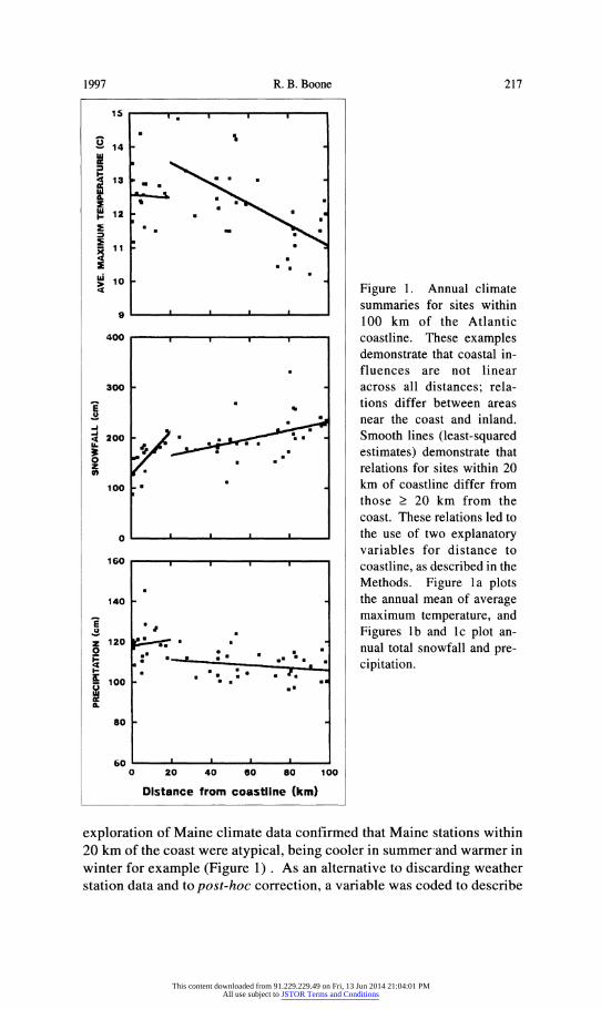
Figure 1. Annual climate summaries for sites within 100 km of the Atlantic coastline. These examples demonstrate that coastal in? fluences are not linear across all distances; rela? tions differ between areas near the coast and inland. Smooth lines (least-squared estimates) demonstrate that relations for sites within 20 km of coastline differ from those > 20 km from the coast. These relations led to the use of two explanatory variables for distance to coastline, as described in the Methods. Figure la plots the annual mean of average maximum temperature, and

Figures lb and lc plot an? nual total snowfall and pre? cipitation.

exploration of Maine climate data confirmed that Maine stations within 20 km of the coast were atypical, being cooler in summer and warmer in winter for example (Figure 1) . As an alternative to discarding weather station data and to post-hoc correction, a variable was coded to describe




coastal sites, with stations > 20 km from the coast assigned 0. Those <

20 km were assigned 0 to 1, based on distance to coastline [i.e., (20.0 -

distance to coastline) / 20.0].

Response Variables The climatic variables modeled (Table 1) included temperature ex?

tremes, precipitation, and measures of productivity. Mean temperature may seem an intuitive measure, but that information was unavailable, and the daily mean of the minimum and maximum temperatures would be

misleading and would not add information. Only 3 weather stations

reported actual evaporation, so that variable was not modeled. Many weather stations did not include data for the entire 30-year period of interest from 1964 to 1993. Balancing the need to exclude sites with short

survey periods with the need to represent the state adequately was diffi? cult. Sites with few years of observations may have large standard errors.

Including these data in regression models was deemed more favorable than excluding too many weather stations (Thiebaux and Pedder 1987).

Exploratory analyses (scatter plots of climate variables against years sites were observed) suggested that sites with 3 or more years of data were

adequately represented. Weather stations with < 3 years of usable data were discarded from analyses (Briggs and Lemin 1992).

Data for the temperature, snowfall, and precipitation variables were

grouped into the four commonly implemented seasons (winter: D-J-F;

spring: M-A-M; summer: J-J-A; fall: S-O-N) and an annual summary (Van Groenewoud 1984; Briggs and Lemin 1992). For mean and extreme maximum and minimum temperatures, the mean temperature for each season and the annual summary was calculated. For snowfall and precipitation, the total for each time period was used. Summaries

Table 1. Climatic variables modeled using regression, and interpolated through? out Maine. Unless noted, models were developed for each variable for winter (December to February), spring (March to May), summer (June to August), fall

(September to November), and the entire year.

Variable Units Notes

Mean maximum temperature ?C Extreme maximum temperature ?C Mean minimum temperature ?C Extreme minimum temperature ?C Total precipitation cm Total snowfall cm Frost-free period days Potential evapotranspiration cm Heat accumulation ?C days

High during each 24-hr period Maximum of highs per season/year Low during each 24-hr period Minimum of lows per season/year Including melted snow Summer not modeled Annual summary only Winter not modeled 4.4 ?C base threshold



1997 R. B. Boone 219

for seasons were discarded if based upon < 80 days (of ? 90 days) of

data, and annual summaries were discarded if based upon < 325 days. Frost-free period was calculated by summing the number of days with minimum temperature > 0 ?C, between the last spring freeze and the first fall freeze. Heat accumulation is biologically relevant because the

growth and productivity of biological systems is often related to the amount of heat in a system. An index to heat accumulation may be calculated by summing the number of degree-days throughout a period that are above some threshold temperature. The method of calculating heat accumulation that is typical, that of Baskerville and Emin (1969), was employed here using a base threshold of 4.4 ?C. In their method,

changing day length is incorporated into the calculation of the index. Potential evapotranspiration was determined using Thornthwaite's

(1948) methods. Thornthwaite used empirical methods to relate tem?

perature and latitude to potential evapotranspiration. After calculating potential evapotranspiration, the results are corrected using multipliers that adjust for varying lengths of months and lengths of days (Thornthwaite 1948). For each of these response variables, annual records were discarded if based upon < 80 days for seasons, and < 325

days for yearly summaries. Finally, annual records were collapsed for each station, and stations discarded if based upon < 3 years.

Modeling Regression analyses were conducted between each of the response

variables and the group of explanatory variables (i.e., distance to coast?

line, coastal index, latitude, longitude, and elevation). The best-fit model was identified manually, using a method similar to backward

stepwise regression (Wilkinson 1990). A near-saturated model, with each of the explanatory variables and two-effect interactions, was calcu? lated first, then parameters were removed until a satisfactory fit, with a moderate number of parameters, was reached. Parameters were then added and subtracted until a best-fit model was achieved. Belsley (1980) and others have warned that collinear explanatory data may bias

coefficients, so methods described in Wilkinson (1990) were used to ensure that collinearity of variables was modest. Autocorrelation within

response data (exhibited by autocorrelated regression residuals) may broaden error estimates associated with correlation coefficients and overall models (Wang and Akabay 1994). To quantify the influence of autocorrelation the Durbin-Watson test (Durbin and Watson 1950; Durbin and Watson 1951) was used. The Durbin-Watson statistic quan? tifies the serial independence of residuals from a least-squares regres? sion model. If residuals are correlated positively, their test statistic d tends to be small. If residuals were negatively correlated (an unlikely scenario), d tends to be large.




Cell-based GIS modeling procedures (ESRI1991) were used to inter?

polate regression results across Maine. The coefficients determined from the regression analyses were entered into ARC/INFO GRID algebraic statements, and statewide grids were calculated for each variable. The

grids were then projected (UTM zone 19, NAD 1927, Clarke spheroid 1866) and figures were produced. In their final projection, each grid of climatic estimates includes ~ 24,500 cells, each 1,853 m x 1,853 m.

RESULTS

There were 107 active weather stations in Maine from 1964 to 1993. Of these, 19 had too few records to be included in these analyses. Of the

remaining 88 sites, 85% (75) had > 8 years of observations, and 53% of stations had > 20 years of data. Sixteen stations recorded precipitation and snowfall for the period of interest, but did not report temperatures. Because of this, the number of stations with valid response data differed between temperature and precipitation measures. Models of mean and extreme temperatures included ~72 stations, whereas precipitation mod? els included 85 to 88 stations (Figure 2). Differences in the period summarized (i.e., seasonal or annual) and the algorithms used led to subtle differences in the number of stations used in modeling climatic variables (Table 2). The range of elevations represented by the 88 stations used was from 6 m to 466 m. Weather stations were from 0.8

Figure 2. The spatial arrange? ment of the weather stations used in modeling climate in Maine. Stations used in every model are shown as solid circles. Stations that were used only in snow and precipi? tation models are shown as

partially filled circles.



1997 R. B. Boone 221

Table 2. Results of regression analyses relating climatic variables to elevation, latitude, longitude, and distance to coastline (two variables). The relation between climatic variables and explanatory variables was significant in each case (P< 0.001).

Variable Stations Adjusted modeled Multiple r2 multiple r2 Mean

Standard

Mean maximum temperature (?C) Winter 72 0.944 0.942 -2.09 0.52 Spring 72 0.716 0.704 10.40 0.73 Summer 72 0.583 0.552 24.24 0.78 Fall 72 0.876 0.870 12.80 0.54 Year 72 0.766 0.755 11.38 0.73

Extreme maximum temperature (?C) Winter 72 0.735 0.727 1.64 1.20 Spring 72 0.541 0.521 13.21 1.02 Summer 72 0.473 0.450 26.15 0.98 Fall 72 0.692 0.678 15.49 1.02 Year 71 0.828 0.818 12.37 0.64

Mean minimum temperature (?C) Winter 72 0.809 0.800 -13.92 1.42 Spring 72 0.787 0.778 -1.89 0.98 Summer 72 0.636 0.626 11.38 0.92 Fall 72 0.728 0.716 1.79 1.00 Year 72 0.769 0.759 -0.60 1.03

Extreme minimum temperature (?C) Winter 72 0.653 0.638 -19.65 2.21 Spring 72 0.744 0.733 -4.75 1.21 Summer 72 0.582 0.569 9.08 1.18 Fall 72 0.658 0.643 -0.73 1.26 Year 71 0.748 0.737 -1.81 1.18

Precipitation (cm) Winter 88 0.735 0.729 24.35 2.69 Spring 88 0.538 0.527 25.56 3.18 Summer 88 0.412 0.391 27.69 2.11 Fall 88 0.571 0.545 28.94 2.20 Year 87 0.567 0.546 106.15 8.49

Snowfall (cm) Winter 85 0.526 0.509 145.97 19.65 Spring 85 0.547 0.524 50.31 10.50 Fall 85 0.713 0.702 17.81 5.85 Year 85 0.594 0.579 216.86 32.98

Heat accumulation (?C days) Winter 71 0.767 0.756 5.82 2.30 Spring 71 0.543 0.522 351.50 49.29 Summer 71 0.744 0.720 1761.70 98.18 Fall 72 0.834 0.830 536.12 46.65 Year 71 0.757 0.739 2639.13 183.05

Potential evapotranspiration (cm) Spring 72 0.608 0.596 9.70 0.65 Summer 72 0.604 0.568 34.79 0.89 Fall 72 0.878 0.872 11.20 0.52 Year 72 0.786 0.773 55.69 1.59

Frost-free period (days) Year 69 0.635 0.618 125.07 16.13




o 2

? 1

Q |-J-1-1-1-|-1-1-1-J-1-1?

S |-,-,-,-,-,-,-,-,-,-,-p-

0.4 0.5 0.0 0.7 0.8 0.9

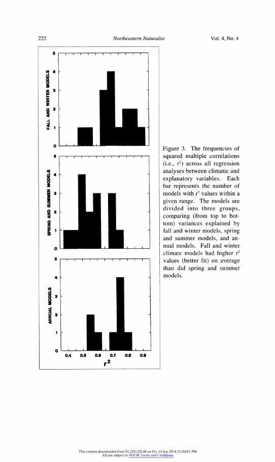
Figure 3. The frequencies of

squared multiple correlations (i.e., r2) across all regression analyses between climatic and

explanatory variables. Each bar represents the number of models with r2 values within a

given range. The models are divided into three groups, comparing (from top to bot? tom) variances explained by fall and winter models, spring and summer models, and an? nual models. Fall and winter climate models had higher r2 values (better fit) on average than did spring and summer models.



1997 R. B. Boone 223

km to 254 km from the Atlantic Ocean.

Three of the 39 models exhibited autocorrelated residuals [winter mean maximum temperature (d=1.43, ^ 72,k=3=1.52), spring extreme minimum temperature (d=l.36, dxl2f^=3=l.52), and spring precipitation (d=1.36, ^i, 88, k=2 =161), see Durbin and Watson (1951)]. Four other models yielded Durbin-Watson d values that were inconclusive. The residuals from the remaining 32 models were not autocorrelated. Mod? els that include autocorrelation still yield unbiased estimates of coeffi?

cients (Mauer 1994; Wang and Akabay 1994), but can broaden error estimates and bias future predictions. Methods of adjusting for autocorrelation are available (Wilson 1992), however they are more

complex than ordinary least squares algorithms. Because these models are themselves not biased and are not intended to predict site-specific future climate, and because autocorrelation was detected in only 8% of

models, ordinary least squares methods were used in this modeling. The percentage of spatial variation in climatic variables that could be

associated with the explanatory variables varied from 41.2% to 94.4%

(Table 2). In general, the squared multiple correlations were distributed

bimodally (Figure 3), with fall and winter r2 values being high (e.g., 0.94 to 0.53; % = 0/74) and spring and summer r2 values being lower

(e.g., 0.79 to 0.41; % = 0.60) on average (P=0.002). Variation in the mean maximum and minimum temperatures tended to be explained more fully (i.e., r2 ~ 0.94 to 0.58; % = 0.76) than the averaged extremes of those variables (r2 ? 0.83 to 0.47; % = 0.67) (P=0.059). As in

Ollinger et al._(1995), models of precipitation had lower r2 values (r2 ~

0.41 to 0.74; % = 0L58) than models of temperature means and extremes

(r2 ? 0.94 to 0.47; % = 0.70) (P=0.03), likely due to sources of variation not modeled, such as rain shadow effects (Dingman 1981).

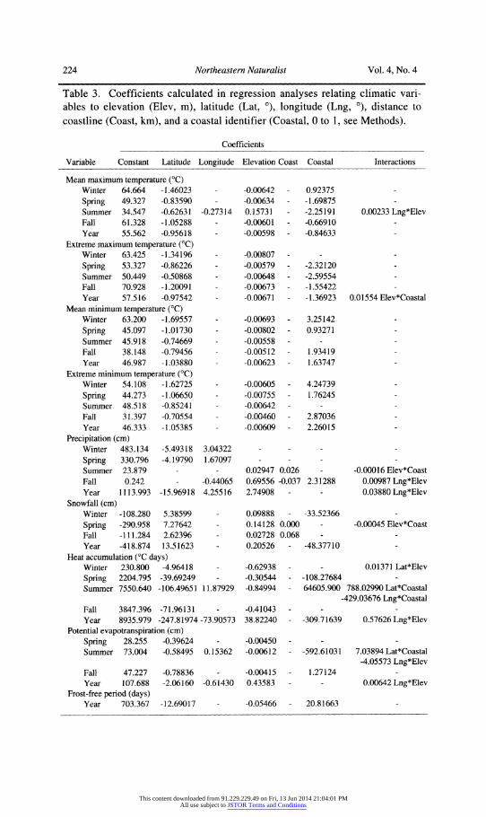
Table 3 reports the correlation coefficients for each of the models

developed. Some of the models were extremely simple; 83% of the variation in fall heat accumulation could be explained using only lati? tude and elevation, for example. In comparison, the model of the same measure for the summer included six coefficients - the maximum in the models. Of 39 models, 7 included two coefficients, 2 included six

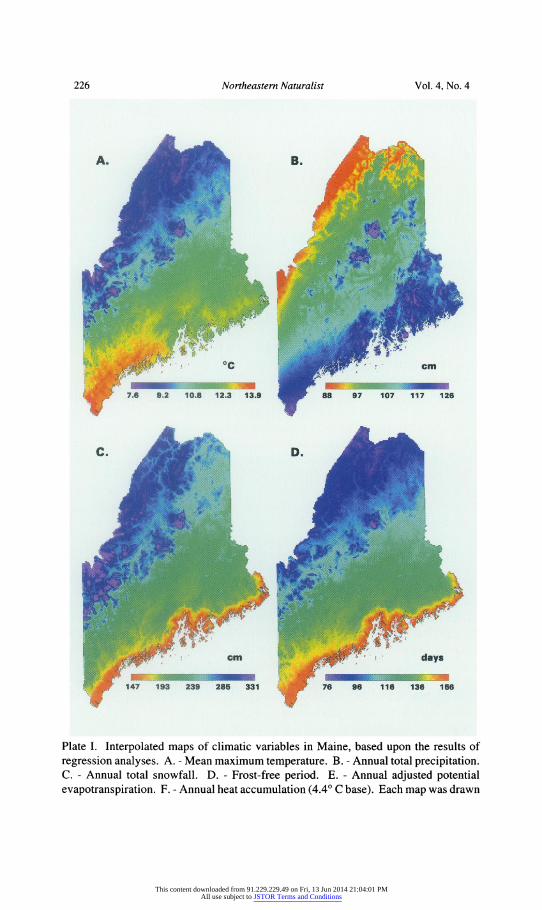
coefficients, and 23 (59%) included 3 coefficients. A sample of interpo? lations across Maine using these coefficients is shown (Plate I).

Because the models contained varying numbers of coefficients (in? cluding interactions), coefficients for variables cannot be directly com?

pared between models, as in Ollinger et al. (1995). However, some

general patterns may be described. Latitude was negatively correlated with each of the climatic variables, except for snowfall, and was in? cluded in 37 of 39 models. Longitude was included in fewer models (9). Others modeling climate also have found longitude to be a weak ex

planatory variable (Leffler 1981). Four of the models including longi-




Table 3. Coefficients calculated in regression analyses relating climatic vari? ables to elevation (Elev, m), latitude (Lat, ?), longitude (Lng, ?), distance to coastline (Coast, km), and a coastal identifier (Coastal, 0 to 1, see Methods).

Coefficients

Variable Constant Latitude Longitude Elevation Coast Coastal Interactions

Mean maximum temperature (?C) Winter Spring Summer Fall Year

64.664 49.327 34.547 61.328 55.562

-1.46023 -0.83590 -0.62631 -1.05288 -0.95618

-0.27314

Extreme maximum temperature (?C) Winter Spring Summer Fall Year

63.425 53.327 50.449 70.928 57.516

-1.34196 -0.86226 -0.50868 -1.20091 -0.97542

Mean minimum temperature (?C) Winter Spring Summer Fall Year

63.200 45.097 45.918 38.148 46.987

-1.69557 -1.01730 -0.74669 -0.79456 -1.03880

Extreme minimum temperature (?C) Winter 54.108 -1.62725 Spring 44.273 -1.06650 Summer 48.518 -0.85241 Fall 31.397 -0.70554 Year 46.333 -1.05385

Precipitation (cm) Winter 483.134 -5.49318 3.04322 Spring 330.796 -4.19790 1.67097 Summer 23.879 Fall 0.242 - -0.44065 Year 1113.993 -15.96918 4.25516

Snowfall (cm) Winter -108.280 5.38599 Spring -290.958 7.27642 Fall -111.284 2.62396 Year -418.874 13.51623

Heat accumulation (?C days) Winter 230.800 -4.96418 Spring 2204.795 -39.69249 Summer 7550.640 -106.49651 11.87929

Fall 3847.396 -71.96131 Year 8935.979 -247.81974-73.90573

Potential evapotranspiration (cm) Spring 28.255 -0.39624 Summer 73.004 -0.58495 0.15362

Fall 47.227 -0.78836 Year 107.688 -2.06160 -0.61430

Frost-free period (days) Year 703.367 -12.69017

-0.00642 -0.00634 0.15731 -0.00601 -0.00598

-0.00807 -0.00579 -0.00648 -0.00673 -0.00671

-0.00693 -0.00802 -0.00558 -0.00512 -0.00623

-0.00605 -0.00755 -0.00642 -0.00460 -0.00609

0.92375 -1.69875 -2.25191 -0.66910 -0.84633

0.00233 Lng*Elev

-2.32120 -2.59554 -1.55422 -1.36923 0.01554 Elev*Coastal

3.25142 0.93271

1.93419 1.63747

4.24739 1.76245

2.87036 2.26015

0.02947 0.69556 2.74908

0.09888 0.14128 0.02728 0.20526

-0.62938 -0.30544 -0.84994

-0.41043 38.82240

-0.00450 -0.00612

-0.00415 0.43583

-0.05466

0.026 - -0.00016 Elev*Coast -0.037 2.31288 0.00987 Lng*Elev

0.03880 Lng*Elev

- -33.52366 0.000 - -0.00045 Elev*Coast 0.068

- -48.37710

0.01371 Lat*Elev -108.27684 64605.900 788.02990 Lat*Coastal

-429.03676 Lng*Coastal

-309.71639 0.57626 Lng*Elev

-592.61031 7.03894 Lat*Coastal -4.05573 Lng*Elev

1.27124 0.00642 Lng*Elev

20.81663



1997 R. B. Boone 225

tude described precipitation, which increases as one moves from west to east in Maine. Elevation is included in all but two of the models of climate. Temperature variables (including heat accumulation, evapora? tion, and frost-free period) are negatively related to elevation in general, and precipitation and snowfall were positively associated - higher areas are cooler and wetter than lower areas (see Daly et al. 1994). Distance to coastline was included in only four of the models of precipitation. In

contrast, the coastal variable, which identifies areas within 20 km of the

coastline, was included in 26 of 39 models. For climatic variables associated with temperature, ocean affects appear limited to a narrow band (~ 20 km) along the immediate coastline.

DISCUSSION

Models of winter, fall, and annual 30-year summaries of temperature extremes, precipitation, and measures of productivity explained ~ 94% to ~ 57% of the variation in climatic data. Models for spring and summer climatic conditions explained less of the variation, from ~ 74% to ~ 41%. Local heating and cooling are more important during summer than other seasons (Daly et al. 1994; Ollinger et al. 1995), as is reflected in the lower r2 values. Regression models of indicators of productivity (i.e., heat accumulation and potential evapotranspiration) and precipita? tion were more complex during summer than other seasons. These climatic responses result from local convective instabilities in summer, whereas in other seasons responses are from broad-scale frontals, and so

vary at a finer spatial resolution during summer than during other seasons (e.g., Daly et al. 1994). Differences in local conditions, such as in vegetation and exposed soils, are also more pronounced in summer. Caution must be used when drawing conclusions about the simplicity of

patterns from these results, however, given that models explained varia? tion in the data to different extents.

These models were developed so that state-wide distributions of terrestrial vertebrates could be compared to climatic variables. Because the distribution of vertebrates may be determined, in part, by environ? mental extremes (e.g., Wiens 1977; Morrison et al. 1992:28-29), mod? els of the deviation of climatic variables from their means (e.g., Marzluff et al. 1994) were sought. However, early exploratory data

analyses of temperature variations demonstrated that regression meth? ods did not model deviations well. In a near-saturated model, < 40% of the variation in the deviations from mean maximum temperature was

explained. After identifying a reasonably parsimonious model, little variation was explained. In general, deviations in temperature from a

30-year mean were weakly associated with latitude, longitude, eleva? tion, and distance to coastline.

Although the weather station with the highest elevation was 466 m,




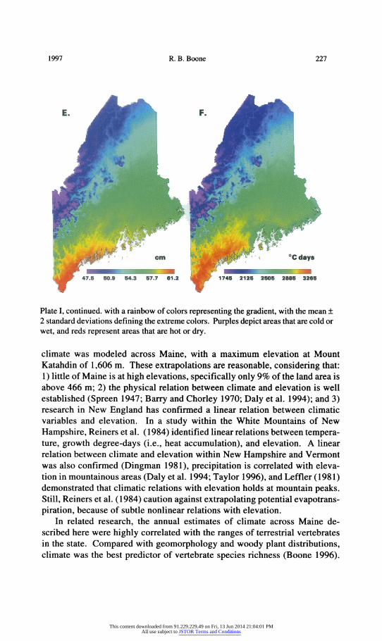
Plate I. Interpolated maps of climatic variables in Maine, based upon the results of regression analyses. A. - Mean maximum temperature. B. - Annual total precipitation. C. - Annual total snowfall. D. - Frost-free period. E. - Annual adjusted potential evapotranspiration. F. - Annual heat accumulation (4.4? C base). Each map was drawn



1997 R. B. Boone 227

Plate I, continued, with a rainbow of colors representing the gradient, with the mean ? 2 standard deviations defining the extreme colors. Purples depict areas that are cold or wet, and reds represent areas that are hot or dry.

climate was modeled across Maine, with a maximum elevation at Mount Katahdin of 1,606 m. These extrapolations are reasonable, considering that:

1) little of Maine is at high elevations, specifically only 9% of the land area is above 466 m; 2) the physical relation between climate and elevation is well established (Spreen 1947; Barry and Chorley 1970; Daly et al. 1994); and 3) research in New England has confirmed a linear relation between climatic variables and elevation. In a study within the White Mountains of New

Hampshire, Reiners et al. (1984) identified linear relations between tempera? ture, growth degree-days (i.e., heat accumulation), and elevation. A linear relation between climate and elevation within New Hampshire and Vermont was also confirmed (Dingman 1981), precipitation is correlated with eleva? tion in mountainous areas (Daly et al. 1994; Taylor 1996), and Leffler (1981) demonstrated that climatic relations with elevation holds at mountain peaks. Still, Reiners et al. (1984) caution against extrapolating potential evapotrans? piration, because of subtle nonlinear relations with elevation.

In related research, the annual estimates of climate across Maine de? scribed here were highly correlated with the ranges of terrestrial vertebrates in the state. Compared with geomorphology and woody plant distributions, climate was the best predictor of vertebrate species richness (Boone 1996).




In multiple linear regression, climatic variation explained 78% of varia? tion in richness of all species, and in tree regression (a method of

regression using recursive binary splitting of data), 92% of the variation in richness was explained (see Boone 1996 for details). These analyses were for the entire state, at a broad-scale (based upon 18 km x 18 km

blocks) and correlations at finer scales would be lower, but the utility of the climate models for broad-scale analyses was demonstrated.

In describing the results of analyses, lower r2 values were attributed to local sources of variation. Alternatively, regional sources of varia? tion not described by the explanatory variables used may be leading to lower correlations. Comparisons between smoothed maps (e.g., kriged climatic data) and maps from these regression models would indicate the magnitude of local and regional variation. In other research, these

analyses could be repeated periodically, to allow spatial comparisons of Maine's climate through time. Researchers conducting analyses may use the coefficients reported here, and a cell-based GIS system, to easily develop statewide models of temperature extremes, precipitation, and

productivity from 1964 to 1993. In addition, those interested in calcu?

lating estimates for a single site for that time period may do so using the coefficients reported. The method used to do statewide and site calcula? tions is described in the Appendix.

ACKNOWLEDGMENTS

I thank William A. Halteman, Department of Mathematics and Statistics, University of Maine, for advice on statistical methods. The reviews of William B. Krohn, Malcolm L. Hunter, Jr., and M. Kate Beard-Tisdale, and two

anonymous reviewers greatly improved the manuscript and are appreciated. This research was supported by The Gap Analysis Program of the U.S. Geologi? cal Survey, Biological Resources Division. The use of trade names does not

imply endorsement by the Federal government. This is Scientific Contribution No. 2156 from the Maine Agricultural and Forest Experiment Station.

LITERATURE CITED

ALLEN, J.A. 1871. On the mammals and winter birds of east Florida, with an examination of certain assumed specific characters of birds, and a sketch of the bird-faunae of eastern North America. Bull. Mus. Comp. Zool. 2:161-454.

ANDREWARTHA, H.G. and L.C. BIRCH. 1954. The distribution and abundance of animals. University of Chicago Press, Chicago, Illinois., USA. 782 pp.

BARRY, R.G. and RJ. CHORLEY. 1970. Atmosphere, weather, and climate. Holt, Rinehart, and Winston, Inc. New York, New York. 320 pp.

BASKERVILLE, G.L. and P. EMIN. 1969. Rapid estimation of heat accumulation from maximum and minimum temperatures. Ecology 50:514-517.

BOONE, R.B. 1996. An assessment of terrestrial vertebrate diversity in Maine. Ph.D. Thesis, University of Maine, Orono, Maine. 222 pp.

BRIGGS, R.D. and R.C. LEMIN, JR. 1992. Delineation of climatic regions in Maine. Can. J. For. Res. 22:801-811.

BELSLEY, D.A. 1980. Regression diagnostics: identifying influential data and sources of collinearity. John Wiley and Sons, New York, New York, USA. 292 pp.



1997 R. B. Boone 229

CLARK, I.C. 1979. Practical geostatistics. Applied Science Publishers Ltd., Lon? don, UK. 129 pp.

DALY, C, R.P. NEILSON, and D.L. PHILLIPS. 1994. A statistical-topographic model for mapping climatological precipitation over mountainous terrain. J. Appl. Meteoro. 33:140-158.

DINGMAN, S.L. 1981. Elevation: a major influence on the hydrography of New Hampshire and Vermont, USA. Hydrol. Sci. Bull. 26:399-413.

DURBIN, J. and G.S. WATSON. 1950. Testing for serial correlation in least squares regression I. Biometrica 37:409-428.

DURBIN, J. and G.S. WATSON. 1951. Testing for serial correlation in least squares regression II. Biometrica 38:159-178.

EARTHINFO, INC. 1995. Database guide for Earthlnfo CD2 NCDC Summary of the Day. Earthlnfo, Inc, Boulder, Colorado, USA. 46 pp.

ENVIRONMENTAL SYSTEMS RESEARCH INSTITUTE. 1991. Cell-based mod? eling with GRID. Environmental Systems Research Institute, Redlands, Califor? nia, USA. 336 pp.

HUGGETT,R.J. 1991. Climate, Earth processes and Earth history. Springer-Verlag, New York, New York, USA. 281 pp.

KAREIVAS, P.M. and M. ANDERSEN. 1988. Spatial aspects of species interac? tions: The wedding of models and experiments. Pages 38-54 in Community ecology. A. Hastings (ed.) Springer-Verlag, New York, USA. 131 pp.

KENDEIGH, S.C. 1954. History and evaluation of various concepts of plant and animal communities in North America. Ecology 35:152-171.

KROHN, W.B., K.D. ELOWE, and R.B. BOONE. 1995. Relations among fishers, snow, and martens: Development and evaluation of two hypotheses. For. Chron. 71:97-105.

LEFFLER, R.J. 1981. Estimating average temperature on Appalachian summits. J. Appl. Meteor. 20:637-642.

LINDZEN, R.S. 1990. Dynamics in atmospheric physics. Cambridge University Press, Cambridge, Massachusetts. 310 pp.

MERRIAM, C.H. 1894. Laws of temperature control of the geographic distribution of terrestrial animals and plants. Nat. Geogr. Mag. 6:229-238.

MARZLUFF, J.M., R.B. BOONE, and G.W. COX. 1994. Historical changes in popula? tions and perceptions of native pest birds in the West. Stud. Avian Biol. 15:202-220.

MAURER, BA. 1994. Geographical population analysis: tools for the analysis of biodiversity. Blackwell Scientific Publications, Boston, MA, USA. 130 pp.

MCMAHON, J.S. 1990. The biophysical regions of Maine: patterns in the landscape and vegetation. M.S. Thesis, University of Maine. Orono, Maine, USA. 120 pp.

MORRISON, M.L., B.G. MARCOT, and R.W. MANNAN. 1992. Wildlife-habitat relationships. Univ. of Wisconsin Press, Madison, Wisconsin, USA. 343 pp.

OLLINGER, S.V., J.D. ABER, CA. FEDERER, G.M. LOVETT, and J.M. ELLIS. 1995. Modeling physical and chemical climate of the northeastern United States for a geographical information system. U.S. Dept. of Agriculture, Forest Service. Northeastern Forest Experiment Station, General Technical Report NE-191. 30 pp.

OWEN, J.G. 1990. Patterns of mammalian species richness in relation to tempera? ture, productivity, and variance in elevation. J. Mammal. 71:1-13.

REINERS, W.A., D.Y. HOLLINGER, and G.E. LANG. 1984, Temperature and evapotransiration gradients of the White Mountains, New Hampshire, U.S.A. Arct. Alp. Res. 16:31-36.

ROOT, T. 1988. Energy constraints on avian distributions and abundance. Ecology 69:330-339.

SPREEN, W.C. 1947. A determination of the effect of topography upon precipita? tion. Trans. Amer. Geoph. Union 28:285-290.




STARR, V.P. 1956. The general circulation of the atmosphere. Sci. Amer. 165(6):40-45. TAYLOR, W.G. 1996. Statistical relationships between topography and precipita?

tion in a mountainous area. Northwest Sci. 70:164-178. THIEBAUX, H.J. and M.A. PEDDER. 1987. Spatial objective analysis: with applica?

tions in atmospheric science. Academic Press, New York, New York. 295 pp. THORNTHWAITE, C.W. 1948. An approach toward a rational classification of

climate. Geogr. Rev. 38:55-94. VAN GROENEWOUD, H. 1984. The climatic regions of New Brunswick: a

multivariate analysis of meteorological data. Can. J. For. Res. 14:389-394. WALLACE, J.M. and P.V. HOBBS. 1977. Atmospheric science. Academic Press,

New York, New York. 467 pp. WANG, C.S. and C.K. AKABAY. 1994. Autocorrelation: problems and solutions in

regression modeling. J. Business Forecasting, Winter: 18-26. WIENS, J.A. 1977. On competition and variable environments. Am. Sci. 65:590-97. WILKINSON, L. 1990. SYSTAT: The system for statistics. Evanston, IL, USA. 677 pp. WILSON, A.C. 1992. The effect of autocorrelation on regression-based model

efficiency and effectiveness in analytical review. Auditing 11:32-46. WRIGHT, D.H. 1983. Species-energy theory: an extension of species-area theory.

Oikos 41:496-506.

APPENDIX

To estimate climatic measures for a location in Maine for 1964 to 1993 using the methods described here, one must determine the five explanatory variables for the site. A GIS system or paper maps may be used to determine: 1) elevation, in meters; 2) latitude, in decimal degrees; 3) longitude, in decimal degrees (and negative because of Maine being west of 0?); 4) the distance to the nearest coastline; and 5) the distance to coastline standardized to 0-1, if < 20 km [i.e., (20.0 - distance to coastline) / 20.0]. For example, using a GIS system one may determine that a point near the center of the town of Millinocket is at 122 m elevation (Elev), 45.66? latitude (Lat), -68.71? longitude (Lng), and 127.63 km to the nearest coastline (i.e., Penobscot Bay) (Coast). Because Millinocket is > 20 km from the coastline, the coastal index (Coastal) is 0.

The form and coefficients in the model of interest may be determined from Table 3. To estimate mean maximum annual temperature in Millinocket, for example, Table 3 indicates that the model is:

Temperature = 57.516 + (-0.97542 * Lat) + (-0.00671 * Elev) + (-1.36923 * Coastal) + (0.01554* Coastal * Elev)

From this, it follows that distance to coastline (Coast) and longitude (Lng) did not help to explain variation in extreme maximum temperature in the state. Using the values determined for Millinocket, the value may be estimated:

Temperature = 57.516 + (-0.97542 * 45.66) + (-0.00671 * 122) + (-1.36923 * 0) + (0.01554*0* 122)

Temperature = 57.516 - 0.81862 - 44.53767 + 0 + 0 Temperature = 12.16 ?C = mean maximum temperature for Millinocket, 1964 to 1993.

If a raster-based GIS is available, and statewide estimates of climate are required, the grids described here may be recreated by first: 1) acquiring a DEM for the state, 2) developing latitude and longitude grids as described in the Methods, and 3) developing grids that represent distance to coastline, and a coastal index, as described in the Methods. With these grids in-place, climate may be estimated using raster algebra, which yields a model like that shown for extreme maximum tempera? ture. In ARC/INFO GRID, the commands:

setcell lat setmask elev tmaxmxyr = 57.516 + (-0.00671 * elev) + (-0.97542 * lat) + (-1.36923 * coastal)

+ (0.01554 * coastal * elev) will create a grid called TMAXMXYR that includes estimates of extreme maximum temperature for each cell in the state. Projecting that grid to the projection required will complete the process.



modeling the climate of maine for use in broad-scale ecological analyses

Documents