Modeling TCP LatencyNeal Cardwell, Stefan Savage, Thomas Andersonfcardwell, savage, tomg@cs.washington.edu

Department of Computer Science and EngineeringUniversity of WashingtonSeattle, WA 98195 USA

Abstract—Several analytic models describe the steady-state throughputof bulk transfer TCP flows as a function of round trip time and packetloss rate. These models describe flows based on the assumption that theyare long enough to sustain many packet losses. However, most TCP trans-fers across today’s Internet are short enough to see few, if any, losses andconsequently their performance is dominated by startup effects such asconnection establishment and slow start. This paper extends the steady-state model proposed in [34] in order to capture these startup effects. Theextended model characterizes the expected value and distribution of TCPconnection establishment and data transfer latency as a function of trans-fer size, round trip time, and packet loss rate. Using simulations, con-trolled measurements of TCP transfers, and live Web measurements weshow that, unlike earlier steady-state models for TCP performance, our ex-tended model describes connection establishment and data transfer latencyunder a range of packet loss conditions, including no loss.

I. I NTRODUCTION

Many of today’s popular Internet applications, including theWorld-Wide Web, e-mail, file transfer, Usenet news, and remotelogin, use TCP as a transport protocol. As a consequence, TCPcontrols a large fraction of flows, packets, and bytes that travelover wide-area Internet paths [41, 10].

Recently researchers have proposed a number of analyticmodels to characterize TCP performance in terms of round-tripdelay and packet loss rate [12, 24, 18, 27, 22, 25, 21, 34, 30,33, 40, 9]. Beyond achieving a better understanding of the sen-sitivity of TCP performance to network parameters, these mod-els have helped inform the design of active queue managementschemes [13, 32] and TCP-friendly multicast protocols [6, 42].

The analytic models proposed to date can be split into twobroad classes: models for steady-state bulk transfer throughput,and models for short flows that suffer no packet loss.

The majority of models fit in the first class; they focuson characterizing bulk transfer throughput. While these mod-els are very successful at predicting steady-state throughput[5, 38], many recent studies have noted that the majority ofTCP flows traveling over the wide-area Internet are very short,with mean sizes around 10KB and median sizes less than 10KB[11, 4, 23, 16, 41, 10]. Because these flows are so short, theyoften spend their entire lifetime in TCP’s slow start mode, with-out suffering a single loss. Since the steady-state models assumeflows suffer at least one loss, they are undefined for this commoncase.

The second class of models focuses on these short flows thatsuffer no packet losses [18, 24, 35]. However, these modelsdo not consider delayed acknowledgments, sender or receiverbuffering limitations, alternative initial congestion windows, orlosses during connection establishment, each of which can have

a dramatic performance impact.This paper proposes a new model for TCP performance that

integrates the results from both classes of models. In particu-lar, we extend the steady-state results from [34] by deriving newmodels for two aspects that can dominate TCP latency: the con-nection establishment three-way handshake and slow start. Us-ing simulation, controlled measurements, and live Web traceswe show that our new slow start model works well for TCPflows of any length that suffer no packet losses, and the modelfrom [34] often works well for flows of any length that do sufferpacket losses. Thus our combined approach, which integratesthese two models, is appropriate for predicting the performanceof both short and long flows under varying packet loss rate con-ditions. In addition, we suggest a technique for estimating thedistribution of of data transfer latencies.

The rest of this paper is organized as follows. Section II de-scribes the new model and relates it to the models from whichit is descended. Section III compares the connection establish-ment model with simulations and Section IV compares the datatransfer model to simulations, TCP measurements, and HTTPtraces. Finally, Section V summarizes our conclusions.

II. T HE MODEL

A. Assumptions

The extended model we develop here has exactly the sameassumptions about the endpoints and network as the steady statemodel presented in [34]. The following section describes theseassumptions in detail, including a few assumptions not statedexplicitly in [34], since these details can have a large impact onthe latency of short TCP flows. Throughout our presentation ofthis model we use the same terminology and notation as [34].

A.1 Assumptions about Endpoints

First, we assume that the sender is using a congestion controlalgorithm from the TCP Reno family; we refer readers to [37,2, 20] for details about TCP and Reno-style congestion control.While we describe the model in terms of the simpler and morecommon TCP Reno algorithm, it should apply just as well tonewer TCP implementations using NewReno, SACK, or FACK[14, 28, 26]. Previous measurements suggest the model shouldbe even more faithful to these more sophisticated algorithms, asthey are more resilient to bursts of packet losses [27, 5].

Since we are focusing on TCP performance rather than gen-eral client-server performance, we do not model sender or re-

ceiver delays due to scheduling or buffering limitations. Instead,we assume that for the duration of the data transfer, the sendersends full-sized segments (packets) as fast as its congestion win-dow allows, and the receiver advertises a consistent flow controlwindow. Similarly, we do not account for effects from the Naglealgorithm or silly window syndrome avoidance, as these can beminimized by prudent engineering practice [17, 29].

We assume that the receiver has a “typical” delayed acknowl-edgment implementation, whereby it sends an acknowledgment(ACK) for everyb = 2 data segments, or whenever its delayedACK heartbeat timer expires, whichever happens first. AlthoughLinux 2.2, for example, uses a more adaptive implementation ofdelayed ACKs, for very short flows this technique can be mod-eled well with b = 1, and for longer flows the effect of thisapproach is only to shave off at most one or two round trips.

A.2 Assumptions about the Network

We model TCP behavior in terms of “rounds,” where a roundstarts when the sender begins the transmission of a window ofpackets and ends when the sender receives an acknowledgmentfor one or more of these packets. We assume that the time tosend all the packets in a window is smaller than the durationof a round and that the duration of a round is independent ofthe window size. Note that with TCP Reno congestion controlthis can only be true when the flow is not fully utilizing the pathbandwidth.

We assume that losses in one round are independent of thelosses in any other round, while losses in the same round arecorrelated, in the sense that any time a packet is lost, all furtherpackets in that round are also lost. These assumptions are ideal-izations of observations of the packet loss dynamics of paths us-ing FIFO drop-tail queuing [7, 36, 44] and may not hold for linksusing RED queuing [15] or paths where packet loss is largelydue to link errors rather than congestion. We assume that theprobability of packet loss is independent of window size; again,this can only hold for flows that are not fully utilizing a link.

When modeling data transfer, we assume that packet loss hap-pens only in the direction from sender to receiver. This assump-tion is acceptable because low levels of ACK loss have only asmall effect with large windows, and network paths are oftenmuch more congested in the direction of data flow than the di-rection of ACK flow [41, 39]. Because packet loss has a farmore drastic result during connection establishment, we modelpacket loss in both directions when considering connection es-tablishment.

A.3 Assumptions about the Transfer

Though we share the assumptions of [34] about the endpointsand network, we relax several key assumptions about the datatransfer. Namely, we allow for transfers short enough to suffera few packet losses, or zero losses, and thus to be dominated byconnection establishment delay and the initial slow start phase.

SYN x

SYN y, ACK x+1

ACK y+1

ActiveOpener

PassiveOpener

i Failures

j Failures

ConnectionEffectively

Established

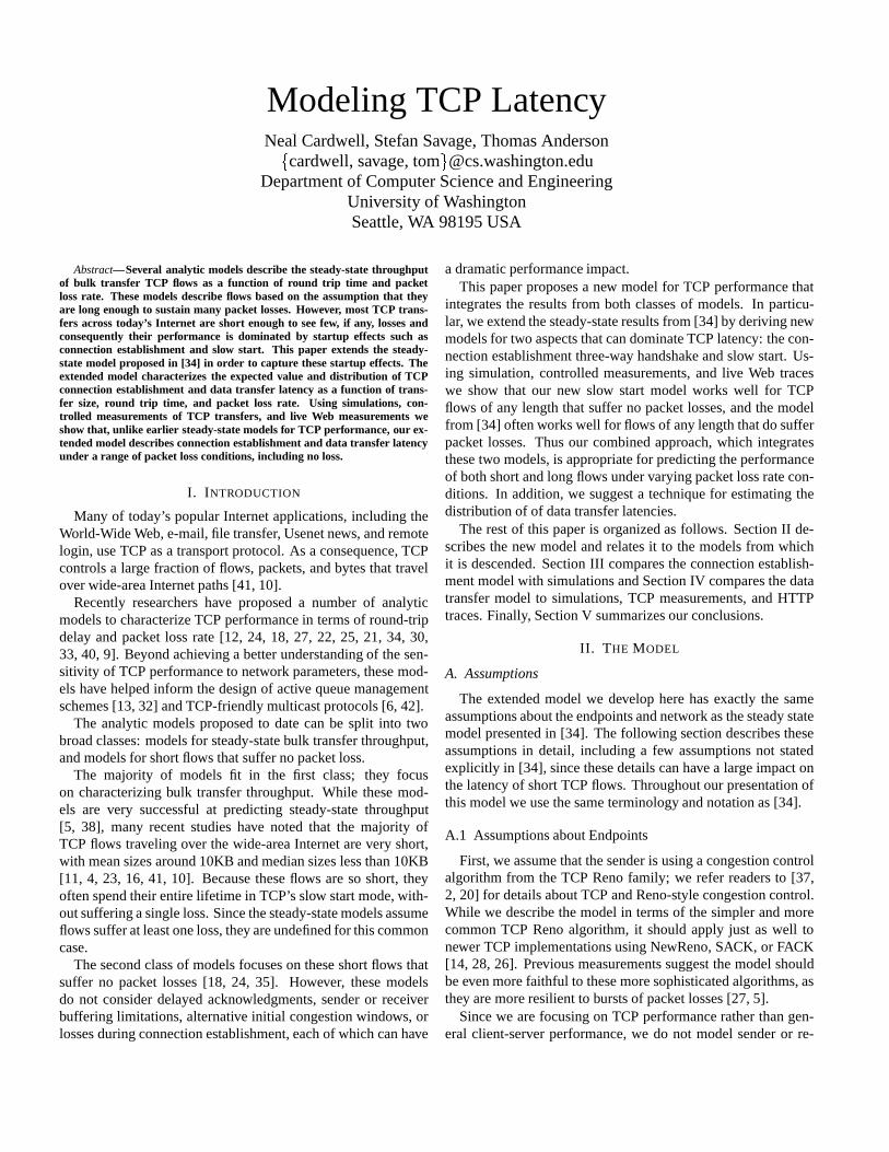
Fig. 1. TCP connection establishment example.

B. Model Overview

Our model describes two aspects of TCP performance. First,we derive expressions for the expected value and distribution oftime required for the connection establishment handshake thatbegins a TCP connection. Second, we derive an expression forthe expected latency to transfer a given amount of data and thendescribe our methodology for extrapolating the distribution ofthis transfer latency. Separating connection establishment la-tency from data transfer latency allows us to apply the modelto applications that establish a single TCP connection and use itfor several independent data transfers.

C. Connection Establishment

Every successful TCP connection begins with a “three-wayhandshake” in which the endpoints exchange initial sequencenumbers. Figure 1 shows an example. The initiating host, typi-cally the client, performs anactive openby sending a SYN seg-ment with its initial sequence number,x. The server performsa passive open; when it receives a SYN segment it replies witha SYN segment of its own, containing its initial sequence num-ber,y, as well as an ACK for the active opener’s initial sequencenumber. When the active opener receives this SYN/ACK packet,it knows that the connection has been successfully established.It confirms this by sending an ACK of the passive opener’s ini-tial sequence number. At each stage of this process, if eitherparty does not receive the ACK that it is expecting within someSYN timeout,Ts, initially three seconds [8], it retransmits itsSYN and waits twice as long for a response.

To model this process in the presence of packet loss in eitherdirection, we definepf as the “forward” packet loss rate alongthe path from passive opener to active opener (“forward” sincethis is usually the primary direction of data flow) andpr as the“reverse” packet loss rate. LetRTT be the average round tripdelay between the two hosts.

Our model of the three-way handshake consists of the follow-ing stages. First, the active opener transmits its SYNi � 0 timesunsuccessfully, until the(i + 1)-th SYN arrives successfully atthe passive opener. Next the passive opener will ignore further

SYNs from the active opener while it repeatedly retransmits itsSYN/ACK until it receives a response. In general it will send itsSYN/ACK j � 0 times unsuccessfully until finally the(j+1)-thSYN/ACK arrives successfully at the active opener. For the pur-poses of the model, we consider the connection to be establishedat this point, since, in most application protocols, immediatelyafter sending the ACKy+1, the active opener sends a data seg-ment to the passive opener that contains a redundant ACKy+1.

Let Ph(i; j) be the probability of having a three-way hand-shake episode consisting of exactlyi failures transmittingSYNs, followed by one successful SYN, followed by exactlyj failures transmitting SYN/ACKs, followed by one successfulSYN/ACK. Then

Ph(i; j) = pir � (1 � pr) � pjf� (1 � pf ) (1)

The latency,Lh(i; j), for this process is

Lh(i; j) = RTT +

i�1Xk=0

2kTs

!+

j�1Xk=0

2kTs

!

= RTT + (2i � 1)Ts + (2j � 1)Ts

= RTT + (2i + 2j � 2)Ts (2)

The probability thatLh, the overall latency for a three-wayhandshake episode, ist seconds or less is:

P [Lh � t] =X

Lh(i;j)�t

Ph(i; j) (3)

Most TCP implementations abort connection establishment at-tempts after 4-6 failures. For loss rates low enough that mosthandshakes succeed before TCP gives up, it can be shown that(4) is a good approximation for the expected handshake time:

E[Lh] = RTT + Ts

�1� pr1� 2pr

+1� pf1� 2pf

� 2

�(4)

This model assumes the TCP implementation complies withthe TCP specification [37]. It does not model non-compliantimplementations, such as current versions of Linux 2.2, thatachieve slightly better performance by responding to retransmit-ted SYN segments with retransmitted SYN/ACK segments.

D. Data Transfer

As defined here, a data transfer begins when an applicationplaces data in its send buffer and ends when TCP receives anacknowledgment for the last byte in the buffer. We assume thatduring this transfer the sending application places data in thesend buffer quickly enough that the sending TCP can send asfast as its window allows.

We decompose the data transfer latency,E[T ], for d data seg-ments into four aspects: the initial slow start phase, the resultingpacket loss (if any), the transfer of any remaining data, and theadded delay from delayed acknowledgments. We begin by cal-culating the amount of data we expect to send in the initial slowstart phase before encountering a packet loss or finishing the

data transfer. From this we can deduce the time spent in slowstart, the final congestion window in slow start, and thus the ex-pected cost of loss recovery, if any. Then we use the steady-statethroughput from [33] to approximate the cost of sending the re-maining data, if any. Finally, we add any extra cost from delayedACKs. We discuss each of these aspects in turn.

D.1 Initial Slow Start

We assume that the transfer is either the first transfer of a con-nection, or a later transfer on a connection that has experiencedno losses yet. Under these circumstances, TCP begins in slowstart mode, where it quickly increases its congestion window,cwnd, until it detects a packet loss.E[Tss], the expected latency for the initial slow start phase,

depends on the structure of the slow start episode. There are twoimportant cases. In the first case, the sender’scwnd grows con-tinuously until it detects a packet loss. In the second case, thesender’scwnd is eventually bounded by a maximum window,Wmax, imposed by sender or receiver buffer limitations. To de-termine which case is appropriate, we need to calculateE[dss],the number of data segments we expect the sender to send beforelosing a segment. From this we can deduceE[Wss], the windowwe would expect TCP to achieve at the end of slow start, werethere no maximum window constraint. IfE[Wss] � Wmax,then the window limitation has no effect, andE[Tss] is simplythe time for a sender to sendE[dss] in the exponential growthmode of slow start. On the other hand, ifE[Wss] > Wmax thenE[Tss] is the time for a sender to slow start up tocwnd = Wmax

and then send the remaining data segments at a rate ofWmax

segments per round.First we calculateE[dss], the number of data segments we

expect to send in the initial slow start phase before a loss occurs(not including the lost segment). Letp be the data segment lossrate. If p = 0, we expect to be able to send alld segments inslow start, soE[dss] = d. On the other hand, ifp > 0, and weassume that the loss rate is independent of sender behavior, then

E[dss] =

d�1Xk=0

(1� p)k � p � k

!+ (1� p)d � d

=(1 � (1 � p)d)(1 � p)

p+ 1 (5)

Next we deduce the time spent in slow start. During slowstart, as always, each round the sender sends as many data seg-ments as itscwnd allows. Since the receiver sends one ACK foreveryb-th data segment that it receives, each round the senderwill get approximatelycwnd=b ACKs. Because the sender is inslow start, for each ACK it receives, it increases itscwnd by onesegment. Thus, if we usecwndi to denote the sender’s conges-tion window at the beginning of roundi and, following [1], use to denote the rate of exponential growth ofcwnd during slowstart , we have:

cwndi+1 = cwndi + cwndi=b

= (1 + 1=b) � cwndi

= � cwndi (6)

If a sender starts with an initialcwnd of w1 segments, thenssdatai, the amount of data sent by the end of slow start round

i, can be closely approximated by a geometric series as

ssdatai = w1 +w1 � + w1 � 2 + � � �+ w1 �

i�1 (7)

= w1 � i � 1

� 1(8)

Solving for i, the number of slow start rounds to transferssdatai segments of data, we arrive at:

i = log

�ssdatai( � 1)

w1+ 1

�(9)

From (7) and (9) it follows thatWss(d), the window TCPachieves after sendingd segments in unconstrained slow start,is

Wss(d) = w1 �

�d( � 1)

w1+ 1

�� �1

=d( � 1)

+w1

(10)

Given typical parameters of = 1:5 and1 � w1 � 3, equa-tion (10) implies thatWss(d) � d

3 . Put another way, to reachany congestion window,w, a flow needs to send approximately3w. Interestingly, this implies that to reach full utilization for abandwidth-delay product like 1.5Mbps� 70ms= 13KBytes, aTCP flow will need to transfer 39KBytes, a quantity larger thanmost wide-area TCP flows transfer. From this it is easy to seewhy many Internet flows spend most of their lifetimes in slowstart, as observed in [3].

From (5) and (10) we can calculate the window size we wouldexpect to have at the end of slow start, if we were not constrainedbyWmax:

E[Wss] =E[dss]( � 1)

+w1

(11)

so we can now determine whether we expectcwnd to be con-strained byWmax during slow start.

If E[Wss] > Wmax then slow start proceeds in two phases.First,cwnd grows up toWmax; from (10) the flow will send

d1 = Wmax � w1

� 1(12)

segments during this phase. From (9), this will take

r1 = log

�Wmax

w1

�+ 1 (13)

rounds. During the second phase, the flow sends the remainingdata at a rate ofWmax packets per round, which will take

r2 =1

Wmax(dss � d1) (14)

rounds.Combining (12), (13), and (14) for the case where when

E[Wss] > Wmax, and using (9) for the simpler case whereE[Wss] � Wmax, the time to sendE[dss] data segments inslow start is approximately

E[Tss] =

8>>><>>>:

RTT ��log

�Wmax

w1

�+ 1+

1Wmax

�E[dss]�

Wmax�w1 �1

��whenE[Wss] > Wmax

RTT � log �E[dss]( �1)

w1+ 1�

whenE[Wss] �Wmax

(15)

D.2 The First LossFor some TCP flows, the initial slow start phase ends with the

detection of a packet loss. Since slow start ends with a packetloss if and only if a flow has at least one loss, the probability ofthis occurrence is:

lss = 1� (1 � p)d (16)

There are two ways that TCP detects losses: retransmissiontimeouts (RTOs) and triple duplicate ACKs. [34] gives a deriva-tion of the probability that a sender in congestion avoidance willdetect a packet loss with an RTO, as a function of packet lossrate and window size. They denote this probability byQ(p; w):

Q(p;w) = min

�1;

(1 + (1� p)3(1� (1� p)w�3))

(1 � (1� p)w)=(1 � (1� p)3)

�(17)

The probability that a sender will detect a loss via triple dupli-cate ACKs is simply1�Q(p; w). AlthoughQ(p; w) was derivedunder the assumption that the sender is in congestion avoidancemode and has an unbounded amount of data to send, our expe-rience has shown that it is equally applicable to slow start andsenders with a limited amount of data. This is largely becauseQ(p; w) is quite insensitive to the rate of growth ofcwnd, andsenders with a limited amount of data are already at high riskfor RTOs because they will usually have small windows. Inpractice, we suspect that the fast recovery strategy used by thesender has a far greater impact; senders using SACK, FACK,or NewReno should be able to achieve the behavior predictedby Q(p; w), while Reno senders will have difficulty achievingthis performance when they encounter multiple losses in a sin-gle round [26, 27].

The expected cost of an RTO is also derived in [34]:

E[ZTO] =G(p)T0

1� p(18)

whereT0 is the average duration of the first timeout in a se-quence of one or more successive timeouts, andG(p) is givenby:

G(p) = 1 + p+ 2p2 + 4p3 + 8p4 + 16p5 + 32p6 (19)

The expected cost of a fast recovery period depends on thenumber of packets lost, the fast recovery strategy of the sender’sTCP implementation, and whether the receiving TCP imple-mentation is returning selective acknowledgment (SACK) op-tions. In the best case, where there is a single loss or the sendercan use SACK information, fast recovery often takes only a sin-gle RTT ; in the worst case, NewReno will require oneRTTfor each lost packet. Our experience indicates that which ofthese possibilities actually occurs is usually not important to themodel’s predictions, so, as in the model of [34], for the sake ofsimplicity, we assume that fast recovery always takes a singleRTT .

Combining these results, the expected cost for any RTOs orfast recovery that happens at the end of the initial slow startphase is:

Tloss = lss ��Q(p;E[Wss]) �E[ZTO]+

(1 �Q(p;E[Wss])) �RTT ) (20)

D.3 Transferring the Remainder

In order to approximate the time spent sending any data re-maining after slow start and loss recovery, we estimate theamount of remaining data and apply the steady-state model from[34].

The amount of data left after slow start and any following lossrecovery is approximately

E[dca] = d� E[dss] (21)

This is only an approximation, because the actual amount ofdata remaining will also depend on where in the window the lossoccurs, how many segments are lost, the size of the congestionwindow at the time of loss,Wmax, and the recovery algorithm.However, since the model seems accurate in most cases evenwith this simplification, for the sake of simplicity we use Equa-tion (21).

When there areE[dca] > 0 segments left to send, we approxi-mate the time to transfer this data using the steady-state through-put model from [33]. This model gives throughput, which wewill denoteR(p;RTT; T0;Wmax), as a function of loss rate,p,round trip time,RTT , average RTO,T0, and maximum windowconstraint,Wmax:

R =

8>>>>>><>>>>>>:

1�pp

+W (p)

2+Q(p;W (p))

RTT ( b2W (p)+1)+

Q(p;W (p))G(p)T01�p

if W (p) < Wmax

1�pp

+Wmax

2+Q(p;Wmax)

RTT ( b8Wmax+

1�ppWmax

+2)+Q(p;Wmax)G(p)T0

1�p

otherwise

(22)

whereQ(p; w) is given in (17),G(p) is given in (19), andW (p)is the expected congestion window at the time of loss eventswhen in congestion avoidance, also from [33]:

W (p) =2 + b

3b+

r8(1 � p)

3bp+

�2 + b

3b

�2(23)

Using these results for the expected throughput, we approxi-mate the expected time to send the remaining data,E[dca] > 0,as

E[Tca] = E[dca]=R(p;RTT; T0;Wmax) (24)

Using a model for steady-state throughput to characterize thecost of transferring the remaining data introduces several errors.

First, when the sender detects a loss in the initial slow startphase, itscwnd will often be much larger than the steady-stateaveragecwnd. Combining (10) and the analysis of [27], thesender will have to detect roughlylog2

1=3pp3=(2bp)

loss indica-

tions to bringcwnd from its value at the end of slow start,1=3p,to its steady state value,

p3=(2bp). For loss rates of 5% and

higher, the sender exits slow start at nearly the steady-state win-dow value, so the error in our approach should be small. Forloss rates of 0.1% and below, it can take three or more loss indi-cations – corresponding to megabytes of data – to reach steadystate, so our approach will often overestimate the latency of suchtransfers.

Another source of error derives from the fact that (22) doesnot model slow start after retransmission timeouts (RTOs). Forloss rates above 1%, the error this introduces should be small,since for these loss rates congestion avoidance has throughputthat is similar to that of slow start after RTOs. For lower lossrates, RTOs should be uncommon. However, when they occur,their long delays may overwhelm the details ofcwnd growth.

Finally, RTO durations vary widely. Using an average RTO tomodel the duration of a specific short TCP flow will introducesignificant error.

D.4 Delayed Acknowledgments

Delayed acknowledgments comprise the final component ofTCP latency that we consider in our model. There are a numberof circumstances under which delayed acknowledgments cancause relatively large delays for short transfers. The most com-mon delay occurs when the sender sends an initialcwnd of 1MSS. In this case the receiver waits in vain for a second seg-ment, until finally its delayed ACK timer fires and it sends anACK. In BSD-derived implementations this delay is uniformlydistributed between 0ms and 200ms, while in Windows 95 andWindows NT 4.0 this delay is distributed uniformly between100ms and 200ms. Delayed ACKs may also lead to large de-lays when the sender sends a small segment and then the Naglealgorithm prevents it from sending further segments [17, 29],or when the sender sends segments that are not full-sized, andthe receiver implementation waits for two full-sized segmentsbefore sending an ACK.

For our simulations and measurements, when senders use aninitial cwnd of 1 MSS we model the expected cost of the first de-layed ACK, which we denoteE[Tdelack], as the expected delaybetween the reception of a single segment and the delayed ACKfor that segment – 100ms for BSD-derived stacks, and 150msfor Windows.

D.5 Combining the ResultsTo model the expected time for data transfer, we use the sum

of the expected delays for each of the components, including(15), (20), (24), and the delayed ACK cost:

E[T ] = E[Tss] + E[Tloss] + E[Tca] +E[Tdelack] (25)

E. Modeling Distributions

The model as given in (25) is a prediction of latency giventhe particular parameters experienced by a particular flow. Inour experience, for a set of transfers of the same size over thesame high bandwidth-delay path, the most important determi-nants of overall latency are the number of losses, the averagetimeout duration, and the cost of delayed ACKs. As a result, toapproximate the distribution of latency for a set of flows, onecan consider the range of possible loss rates and delayed ACKcosts, and estimate the likelihood of each scenario, along withthe latency expected with that scenario. In section IV-A.2 we ap-ply this method to simulations using a Bernoulli loss model anddelayed ACK costs uniformly distributed between 0 and 200ms.

0

100000

200000

300000

400000

500000

600000

700000

800000

900000

1e+06

0.0001 0.001 0.01 0.1 1

Ban

dwid

th (

byte

s/se

c)

Frequency of Loss Indications (p)

Proposed (2 KB)Proposed (64 KB)

Proposed (256 KB)Proposed (1024 KB)

[PFTK98][MSMO97]

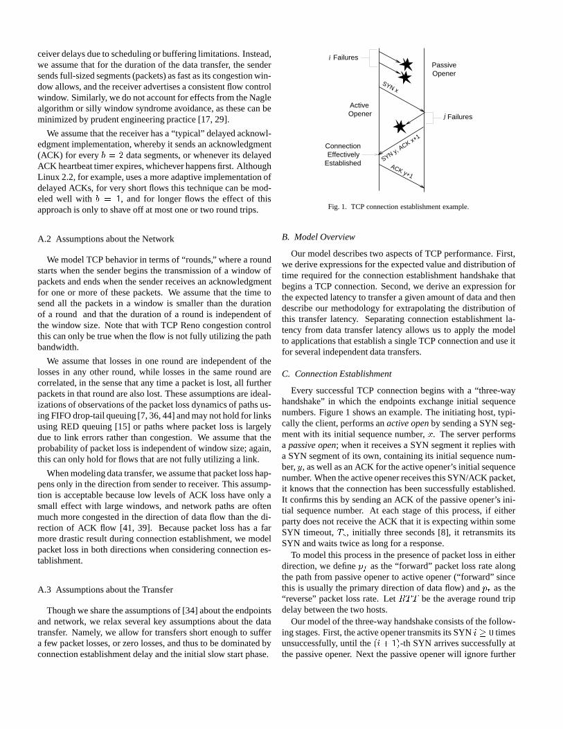
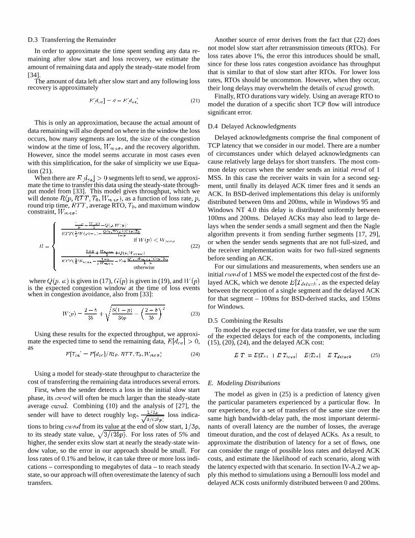
Fig. 2. Comparing the throughput predicted by the steady state models to thethroughput predicted by our proposed model for varying transfer sizes. HereMSS = 1460 bytes,RTT = 100 ms,w1 = 1 segment, = 1:5, T0 = 1sec,Wmax = 10 MBytes.

F. Comparison with Earlier Models

Our proposed model, (25), is a generalization of two previousapproaches. In the case where there are no packet losses, (25)reduces to (15), a model for the time to sendd segments in slowstart mode. This special case corresponds closely to the simplermodels derived in [18, 24]. In the case whered is very large, thetotal time given by (25) is dominated by (24), the time to transferdata after the first loss. In this case, the behavior correspondsvery closely with the underlying throughput model, (22), from[34].

Figure 2 explores the relationship between our proposedmodel and the models of [27] and [34]. It gives the through-put predicted by the proposed model, (25), for each of severaltransfer sizes, as well as the steady-state throughputs predictedby the expression

p3=4�MSS=(RTT

pp), from [27], and (22),

from [34]. As mentioned earlier, when there is at least one ex-pected loss, our proposed model agrees closely with [34], whichhas been shown to work well for flows that suffer even a fewlosses [5]. On the other hand, when there are no losses, the pro-posed model predicts that short flows suffer because they do nothave time to reach a steady-statecwnd, whereas long flows willdo well because theircwnd grows beyond its steady-state value.

III. V ERIFYING THE CONNECTION ESTABLISHMENT

MODEL

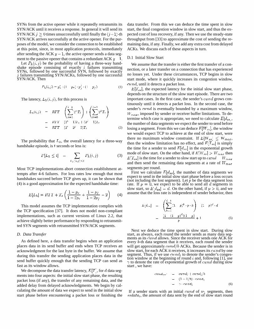
Figure 3 compares the mean and distribution of connectionestablishment times given by (3) and the mean given by theapproximate model (4) to the mean and distribution for 1000ns [31] simulations withRTT = 70 ms and Bernoulli packetlosses withpf = 0:3 andpr = 0:2. These simulations used theFullTCP implementation, modeled closely after the 4.4BSDTCP implementation. Both the model and the approximation fitwell. Results are similar for other scenarios with bothpf andprwell below 0.5.

Figure 4 summarizes the performance of the full and approx-

0

0.2

0.4

0.6

0.8

1

0 5 10 15 20 25

Cum

ulat

ive

Fra

ctio

n

Time (sec)

Simulated CDFModeled CDF

Simulated meanModeled mean

Approximate Model

Fig. 3. Distribution and mean of connection establishment times from the model(3), the approximate model (4), and 1000ns simulations withpf = 0:3,pr = 0:2.

0

2

4

6

8

10

12

0 0.05 0.1 0.15 0.2 0.25 0.3 0.35 0.4 0.45

Tim

e (s

ec)

Forward loss rate

SimulatedModeled

Approximate Model

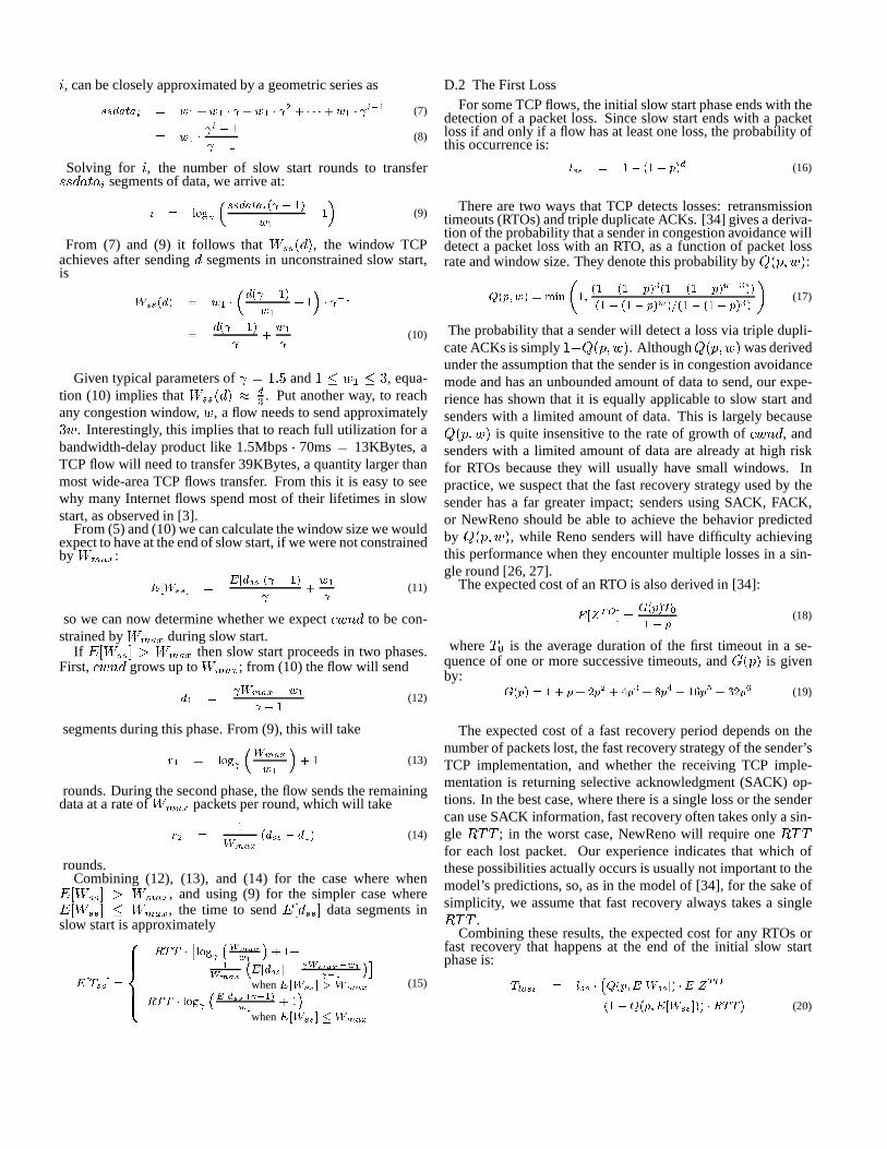
Fig. 4. Expected connection establishment latency fromns simulations (1000trials at each loss rate), the model (3), and the approximate model (4).

imate model, comparing them against 1000ns trials in scenar-ios with pr = 0:0 and0 � pf � 0:45. The full model fitswell across these simulations, but the approximate model di-verges sharply aspf approaches 0.5, where its assumption ofunbounded wait times fails.

IV. V ERIFYING THE DATA TRANSFERMODEL

A. Simulations

A.1 Flows Without Loss

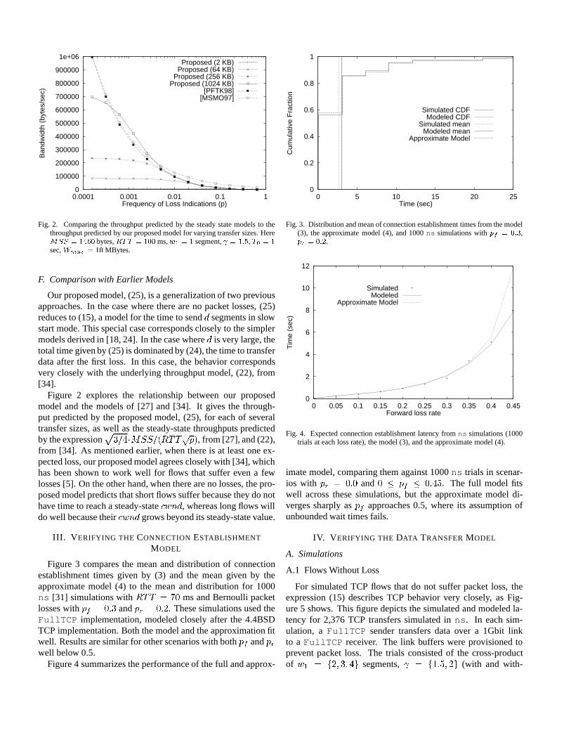
For simulated TCP flows that do not suffer packet loss, theexpression (15) describes TCP behavior very closely, as Fig-ure 5 shows. This figure depicts the simulated and modeled la-tency for 2,376 TCP transfers simulated inns . In each sim-ulation, aFullTCP sender transfers data over a 1Gbit linkto a FullTCP receiver. The link buffers were provisioned toprevent packet loss. The trials consisted of the cross-productof w1 = f2; 3; 4g segments, = f1:5; 2g (with and with-

0

20

40

60

80

100

120

140

160

0 20 40 60 80 100 120 140 160

Mod

eled

Tra

nsfe

r T

ime

(RT

T)

Simulated Transfer Time (RTT)

Modeled TimeSimulated Time

Fig. 5. The simulated latency for 2,376 TCP data transfers that experienced nopacket loss, compared with the modeled latency from (25) (or, equivalently,(15)).

0

100000

200000

300000

400000

500000

600000

1e-05 0.0001 0.001 0.01 0.1 1

Ban

dwid

th (

byte

s/se

c)

Frequency of Loss Indications (p)

SimulatedProposed[PFTK98]

[MSMO97]

Fig. 6. Scatter plot of simulated performance with model predictions over-laid. These were 64 KByte transfers withMSS = 1460 bytes,Wmax of4MBytes,w1 = 1 segment, = 1:5, RTT = 100 ms,T0 = 519 ms,pf = 0:05 andpr = 0.

out delayed ACKs),d = f1; 2; 4; : : :1024g segments,MSS =f536; 1460; 4312g bytes,Wmax = f8; 32; 128; 512g segments,andRTT = f16; 64; 256gms. The model agrees quite closelywith the simulations; the average error is 0.69RTTs, and theaverage relative error is 22%. The three outliers at 37, 72, and143RTTs correspond to trials with a window of just 8 seg-ments, where throughput was hurt because the 200ms delayedACK timer of the recipient was mis-aligned with the 256msRTT ACK-clocking employed by the sender.

A.2 Flows Suffering Losses

Figures 6 and 7 illustrate how well [34] and (25) match theperformance of flows that suffer moderate-to-high levels of loss.Figure 6 shows a scatter plot depicting the bandwidth and lossrate experienced by each of the 100 simulatedFullTCP flows,with the model predictions overlaid. Each flow transferred

0

0.1

0.2

0.3

0.4

0.5

0.6

0.7

0.8

0.9

1

0 0.5 1 1.5 2 2.5 3 3.5 4

Cum

ulat

ive

Fra

ctio

n

Time (sec)

Simulated CDFSimulated (Mean)

[PFTK98]Proposed

Proposed CDF

Fig. 7. The distribution and mean of latencies from the experiment described inFigure 6.

0

500000

1e+06

1.5e+06

2e+06

2.5e+06

1e-05 0.0001 0.001 0.01 0.1 1

Ban

dwid

th (

byte

s/se

c)

Frequency of Loss Indications (p)

SimulatedProposed[PFTK98]

[MSMO97]

Fig. 8. Scatter plot of simulated performance with model predictions over-laid. These were 1 MByte transfers withMSS = 1460 bytes,Wmax of4MBytes,w1 = 1 segment, = 1:5, RTT = 100 ms,T0 = 450 ms,pf = 0:001 andpr = 0.

0

0.1

0.2

0.3

0.4

0.5

0.6

0.7

0.8

0.9

1

0 1 2 3 4 5 6

Cum

ulat

ive

Fra

ctio

n

Time (sec)

Simulated CDFSimulated (Mean)

[PFTK98]Proposed

Proposed CDF

Fig. 9. The distribution and mean of latencies from the experiment described inFigure 8.

0

0.2

0.4

0.6

0.8

1

0 20000 40000 60000 80000 100000 120000

Tra

nsfe

r T

ime

(sec

)

Data Transferred (Bytes)

MeasuredProposed (Slow Start) (15)

Proposed (Full) (25)[PFTK98]

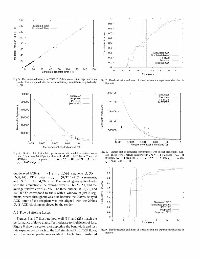
Fig. 10. Measured and modeled latencies for 403 transfers from the Universityof Washington to the UC-Davis.

64KBytes over a path with synthetically-generated Bernoullilosses with an average loss rate ofpf = 0:05 andpr = 0. Theproposed model, (25) fits the trials that experience no packetloss, while both [34] and (25) provide a reasonable fit to thosetrials that do experience loss. Figure 7 shows the distribution oflatencies for these trials. Both [34] and (25) capture the averagelatency, and the modeled distribution, derived using the tech-nique described in Section II-E, provides a reasonable charac-terization of the distribution of latencies. There is considerablevariance in the latency in this case, with 25% of flows complet-ing in half the average time, and 25% of flows taking half againas long as the average time. In our experience, this techniqueyields a good approximation to the latency distribution when-ever there are enough packet losses for [34] to provide a good fitfor the average latency.

Figures 8 and 9 provide the corresponding view of long trans-fers (1 MByte) over paths with low loss rates. The proposedmodel, (25), captures the average latency as well as the latencyexperienced by the half of flows that see no loss. However, nei-ther [34] nor (25) predicts the performance seen by flows thatexperience a single loss, as these flows enter congestion avoid-ance with acwnd far larger than the steady-state value. We havepreliminary results characterizing the dynamics ofcwnd as itconverges to the steady-state value after slow start. It should bepossible to capture aspects of the behavior of these long flowsthat suffer only a few losses by using an approach along theselines.

B. Controlled Internet Measurements

In order to examine how well our proposed model, (25), fitsTCP behavior in the Internet, we performed a number of TCPtransfers from a Linux 2.0.35 sender at the University of Wash-ington to other Internet sites. Figure 10 shows an example.It depicts the latency of 403 transfers of varying sizes to theUniversity of California at Davis, together with the predictionsfrom (25) and [34], using the average packet loss rate acrossall trials. Since the average loss rate was only 0.02%, and as a

0

0.1

0.2

0.3

0.4

0.5

0.6

0.7

0.8

0.9

1

-1 -0.5 0 0.5 1

Cum

ulat

ive

Fra

ctio

n

Error (RTT)

Proposed Model

Fig. 11. The error,(modeled�measured)=RTT , between the proposed model,(25), and the HTTP measurements, for all 33,208 flows (97%) that sufferedno packet losses. Note that this isRTT -normalized error, so the model iswithin 1RTT of the actual time for 85% of flows.

0

0.1

0.2

0.3

0.4

0.5

0.6

0.7

0.8

0.9

1

-1 -0.5 0 0.5 1

Cum

ulat

ive

Fra

ctio

n

Relative Error

Proposed Model[PFTK98]

[MSMO97]

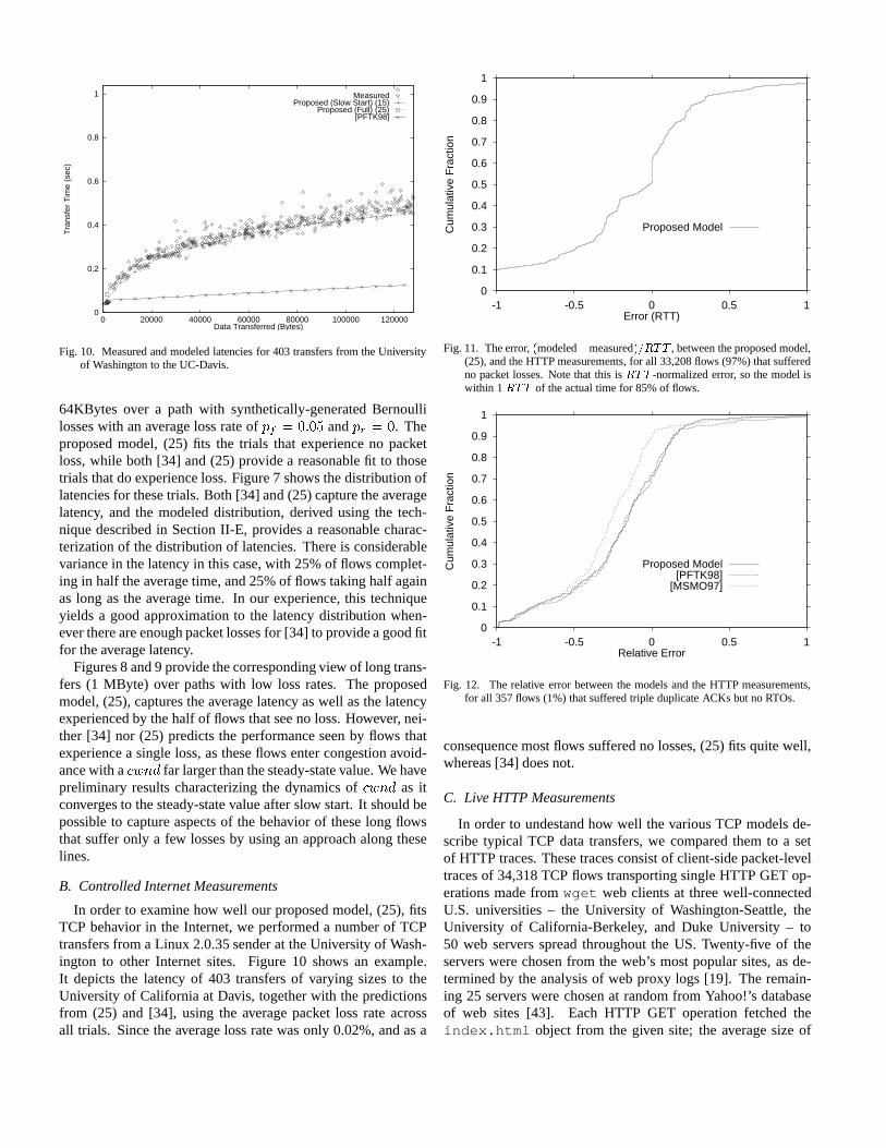
Fig. 12. The relative error between the models and the HTTP measurements,for all 357 flows (1%) that suffered triple duplicate ACKs but no RTOs.

consequence most flows suffered no losses, (25) fits quite well,whereas [34] does not.

C. Live HTTP Measurements

In order to undestand how well the various TCP models de-scribe typical TCP data transfers, we compared them to a setof HTTP traces. These traces consist of client-side packet-leveltraces of 34,318 TCP flows transporting single HTTP GET op-erations made fromwget web clients at three well-connectedU.S. universities – the University of Washington-Seattle, theUniversity of California-Berkeley, and Duke University – to50 web servers spread throughout the US. Twenty-five of theservers were chosen from the web’s most popular sites, as de-termined by the analysis of web proxy logs [19]. The remain-ing 25 servers were chosen at random from Yahoo!’s databaseof web sites [43]. Each HTTP GET operation fetched theindex.html object from the given site; the average size of

0

0.1

0.2

0.3

0.4

0.5

0.6

0.7

0.8

0.9

1

-1 -0.5 0 0.5 1

Cum

ulat

ive

Fra

ctio

n

Relative Error

Proposed Model[PFTK98]

[MSMO97]

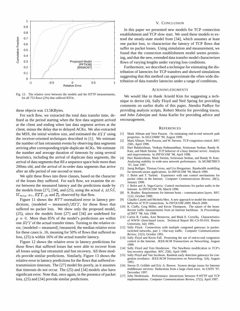
Fig. 13. The relative error between the models and the HTTP measurements,for all 753 flows (2%) that suffered RTOs.

these objects was 13.5KBytes.For each flow, we extracted the total data transfer time, de-

fined as the period starting when the first data segment arrivedat the client and ending when last data segment arrives at theclient, minus the delay due to delayed ACKs. We also extractedthe MSS, the initial window size, and estimated theRTT usingthe receiver-oriented techniques described in [1]. We estimatethe number of fast retransmit events by observing data segmentsarriving after corresponding triple-duplicate ACKs. We estimatethe number and average duration of timeouts by using severalheuristics, including the arrival of duplicate data segments, thearrival of data segments that fill a sequence space hole more than200ms old, and the arrival of in-order data segments that arriveafter an idle period of one second or more.

We split these flows into three classes, based on the characterof the losses they suffered. For each flow, we examine the er-ror between the measured latency and the predictions made bythe models from [27], [34], and (25), using the actuald, MSS,Wmax, w1, RTT , p, andT0 observed by that flow.

Figure 11 shows theRTT -normalized error in latency pre-dictions, (modeled� measured)=RTT , for those flows thatsuffered no packet loss. We show only the proposed model,(25), since the models from [27] and [34] are undefined forp = 0. More than 85% of the model’s predictions are withinoneRTT of the actual transfer times. Turning to the relative er-ror, (modeled�measured)=measured, the median relative errorfor these cases is .16, meaning for 50% of flows that suffered noloss, (25) is within 16% of the actual transfer latency.

Figure 12 shows the relative error in latency predictions forthose flows that suffered losses but were able to recover fromall losses using fast retransmit and fast recovery. All three mod-els provide similar predictions. Similarly, Figure 13 shows therelative error in latency predictions for the flows that suffered re-transmission timeouts. The [27] model fits poorly, as it assumesthat timeouts do not occur. The (25) and [34] models also havesignificant error. Note that, once again, in the presence of packetloss, (25) and [34] provide similar predictions.

V. CONCLUSION

In this paper we presented new models for TCP connectionestablishment and TCP slow start. We used these models to ex-tend the steady-state model from [34], which assumes at leastone packet loss, to characterize the latency of TCP flows thatsuffer no packet losses. Using simulation and measurement, wefound that the connection establishment model seems promis-ing, and that the new, extended data transfer model characterizesflows of varying lengths under varying loss conditions.

Furthermore, we described a technique for estimating the dis-tribution of latencies for TCP transfers and showed simulationssuggesting that this method can approximate the often wide dis-tribution of data transfer latencies under a range of conditions.

ACKNOWLEDGMENTS

We would like to thank Arnold Kim for suggesting a tech-nique to derive (4), Sally Floyd and Neil Spring for providingcomments on earlier drafts of this paper, Jitendra Padhye forproviding analysis scripts, Robert Morris for providing traces,and John Zahorjan and Anna Karlin for providing advice andencouragement.

REFERENCES

[1] Mark Allman and Vern Paxson. On estimating end-to-end network pathproperties. InSIGCOMM ’99, August 1999.

[2] Mark Allman, Vern Paxson, and W. Stevens. TCP congestion control. RFC2581, April 1999.

[3] Hari Balakrishnan, Venkata Padmanabhan, Srinivasan Seshan, Randy H.Katz, and Mark Stemm. TCP behavior of a busy Internet server: Analysisand improvements. InINFOCOM ’98, April 1998.

[4] Hari Balakrishnan, Mark Stemm, Srinivasan Seshan, and Randy H. Katz.Analyzing stability in wide-area network performance. InSIGMETRICS’97, June 1997.

[5] Juerg Bolliger, Thomas Gross, and Urs Hengartner. Bandwidth modellingfor network-aware applications. InINFOCOM ’99, March 1999.

[6] J. Bolot and T. Turletti. Experience with rate control mechanisms forpacket video in the Internet.Computer Communications Review, 28(1),January 1998.

[7] J. Bolot and A. Vega-Garcia. Control mechanisms for packet audio in theInternet. InINFOCOM ’96, March 1996.

[8] R. Braden. Requirements for Internet hosts – communication layers. RFC1122, October 1989.

[9] Claudio Casetti and Michela Meo. A new approach to model the stationarybehavior of TCP connections. InINFOCOM 2000, March 2000.

[10] K. Claffy, Greg Miller, and Kevin Thompson. The nature of the beast:Recent traffic measurements from an Internet backbone. InProceedingsof INET ’98, July 1998.

[11] Carlos R. Cunha, Azer Bestavros, and Mark E. Crovella. Characteristicsof WWW client-based traces. Technical Report BU-CS-95-010, BostonUniversity, July 1995.

[12] Sally Floyd. Connections with multiple congested gateways in packet-switched networks, part 1: One-way traffic.Computer CommunicationsReview, 21(5), October 1991.

[13] Sally Floyd and Kevin Fall. Promoting the use of end-to-end congestioncontrol in the Internet.IEEE/ACM Transactions on Networking, August1999.

[14] Sally Floyd and Tom Henderson. The NewReno modification to TCP’sfast recovery algorithm. RFC 2582, April 1999.

[15] Sally Floyd and Van Jacobson. Random early detection gateways for con-gestion avoidance.IEEE/ACM Transactions on Networking, 1(4), August1993.

[16] Steven D. Gribble and Eric A. Brewer. System design issues for Internetmiddleware services: Deductions from a large client trace. InUSITS ’97,December 1997.

[17] John Heidemann. Performance interactions between P-HTTP and TCPimplementations.Computer Communications Review, 27(2), April 1997.

[18] John Heidemann, Katia Obraczka, and Joe Touch. Modeling the perfor-mance of HTTP over several transport protocols.IEEE/ACM Transactionson Networking, 5(5), October 1997.

[19] http://www.100hot.com/ .[20] Van Jacobson. Congestion avoidance and control.SIGCOMM ’88, August

1988.[21] Anurag Kumar. Comparative performance analysis of versions of TCP in

a local network with a lossy link.IEEE/ACM Transactions on Networking,6(4), August 1998.

[22] T.V. Lakshman and Upamanyu Madhow. The performance of TCP/IPfor networks with high bandwidth-delay products and random loss.IEEE/ACM Transactions on Networking, June 1997.

[23] Bruce A. Mah. An empirical model of HTTP network traffic. InINFO-COM ’97, April 1997.

[24] Jamshid Mahdavi. TCP performance tuning.http://www.psc.edu/networking/tcptune/slides/ , April 1997.

[25] Sam Manthorpe.Implications of the Transport Layer for Network Dimen-sioning. PhD thesis, Ecole Polytechnique Federale de Lausanne, 1997.

[26] M. Mathis and J. Mahdavi. Forward acknowledgement: Refining TCPcongestion control. InSIGCOMM ’96, August 1996.

[27] M. Mathis, J. Semke, J. Mahdavi, and T. Ott. The macroscopic behaviorof the TCP congestion avoidance algorithm.Computer CommunicationsReview, 27(3), July 1997.

[28] Matt Mathis, Jamshid Mahdavi, Sally Floyd, and Allyn Romanow. TCPSelective Acknowledgement options. RFC 2018, April 1996.

[29] Greg Minshall, Yasushi Saito, Jeffrey C. Mogul, and Ben Verghese. Ap-plication performance pitfalls and TCP’s Nagle algorithm. InWorkshopon Internet Server Performance, May 1999.

[30] Archan Misra and Teunis Ott. The window distribution of idealized TCPcongestion avoidance with variable packet loss. InINFOCOM ’99, March1999.

[31] UCB/LBNL/VINT network simulator - ns (version 2).[32] Teunis J. Ott, T. V. Lakshman, and Larry H. Wong. SRED: Stabilized

RED. In INFOCOM ’99, March 1999.[33] Jitendra Padhye, Victor Firoiu, and Don Towsley. A stochastic model of

TCP Reno congestion avoidance and control. Technical Report 99-02,University of Massachusetts, 1999.

[34] Jitendra Padhye, Victor Firoiu, Don Towsley, and Jim Kurose. ModelingTCP throughput: A simple model and its empirical validation. InSIG-COMM ’98, September 1998.

[35] Craig Partridge and Timothy J. Shepard. TCP/IP performance over satel-lite links. IEEE Network, pages 44–49, September/October 1997.

[36] Vern Paxson. End-to-end Internet packet dynamics. InSIGCOMM ’97,September 1997.

[37] Jon Postel, Editor. Transmission Control Protocol — DARPA InternetProgram Protocol Specification. RFC 793, September 1981.

[38] Lili Qiu, Yin Zhang, and S. Keshav. On individual and aggregate TCP per-formance. Technical Report TR99-1744, Cornell University, May 1999.

[39] Stefan Savage. Sting: a TCP-based network measurement tool. InUSITS’99, October 1999.

[40] http://www.ens.fr/˜mistral/tcpworkshop.html , Decem-ber 1998.

[41] Kevin Thompson, Gregory J. Miller, and Rick Wilder. Wide-area Internettraffic patterns and characteristics.IEEE Network, 11(6), November 1997.

[42] L. Vivisano, L. Rizzo, and J. Crowcroft. TCP-like congestion control forlayered multicast data transfer. InINFOCOM ’98, April 1998.

[43] Yahoo! Inc. Random Yahoo! Link.http://random.yahoo.com/bin/ryl .

[44] Maya Yajnik, Sue Moon, Jim Kurose, and Don Towsley. Measurementand modelling of the temporal dependence in packet loss. InINFOCOM’99, March 1999.