Modeling of a hydraulic arresting gear using fluid–structureinteraction and isogeometric analysis

Chenglong Wanga, Michael C.H. Wua, Fei Xua, Ming-Chen Hsua, Yuri Bazilevsb,∗

aDepartment of Mechanical Engineering, Iowa State University, 2025 Black Engineering, Ames, IA 50011, USAbDepartment of Structural Engineering, University of California, San Diego, 9500 Gilman Drive, La Jolla, CA

92093, USA

Abstract

Fluid–structure interaction (FSI) analysis of a full-scale hydraulic arresting gear used to retard theforward motion of an aircraft landing on an aircraft-carrier deck is performed. The simulationsmake use of the recently developed core and special-purpose FSI techniques for other problemclasses, specialized to the present application. A recently proposed interactive geometry modelingand parametric design platform for isogeometric analysis (IGA) is directly employed to create thearresting gear model, and illustrates a natural application of IGA to this problem class. The fluidmechanics and FSI simulation results are reported in terms of the arresting-gear rotor loads andblade structural deformation and vibration. Excellent agreement is achieved with the experimentalresults for the arresting gear design simulated in this work.

Keywords: Fluid–structure interaction; Hydraulic arresting gear; Isogeometric analysis;Parametric design; NURBS; Hydrodynamic loading

1. Introduction

Military aircraft, during landing on the deck of an aircraft carrier, eject a “hook” that engagesa wire connected to a tape drum. The resultant tape-drum angular momentum is transferred tothe rotor inside a hydraulic energy absorber (or a hydraulic arresting gear). The rotor, which isa steel structure several feet in diameter, accelerates rapidly, reaching speeds of 800 rpm. Therotor acceleration is then arrested by the drag forces coming from the surrounding water inside thearresting gear. This, in turn, puts the wire in tension and rapidly slows the aircraft forward motion.The rotor speed and blade topology, geometry, and structural design play a critical role in theperformance of the device, both in its function to arrest the motion of landing aircraft, as well as inits ability to withstand the internal hydrodynamic loads and perform multiple consecutive aircraft

∗Corresponding authorEmail address: yuri@ucsd.edu (Yuri Bazilevs)

The final publication is available at Computers & Fluids via http://dx.doi.org/10.1016/ j.compfluid.2015.12.004

arrests without failure. As a result, accurate prediction of rotor loads and the structure response tothese loads is important, requiring advanced modeling and simulation, which we undertake in thiswork.

Experimental study of the hydraulic arresting gear presents many challenges, which mainlyarise due to the large spatial scales and high rotor speeds involved in the device operation. The factthat the device is completely enclosed complicates the situation further. However, the hydraulicarresting gear lends itself nicely to analysis using computational fluid–structure interaction (FSI).Computational FSI has matured significantly over the last decade and many core and special pur-pose techniques were developed in this arena, which can be used to address the various challengesinvolved in the arresting-gear problem (see, e.g., [1–37] and references therein for a sampling ofFSI methods developed in recent years.)

In addition to FSI, the present application lends itself nicely to Isogeometric Analysis(IGA) [38, 39], which is a relative newcomer to the field of computational mechanics. The use ofIGA enables relatively simple construction of the arresting gear geometric and structural design, itscomplete surface and volume parameterization, and analysis using the same underlying geometricrepresentation in terms of Non-Uniform Rational B-Splines (NURBS) [40] or T-splines [41, 42].

The paper is outlined as follows. In Section 2, we describe the geometry of the Virginia Tech(VT) arresting gear design [43], which belongs to the Model 64 [44] energy absorber system.We describe a novel technique for IGA analysis-suitable geometry construction of the arrestinggear design. We make use of a recently proposed interactive geometry modeling and parametricdesign platform [45], which is based on the Rhino 3D CAD software [46] with an embeddedvisual programming tool Grasshopper [47]. Rhino 3D gives the user access to complex geometrymodeling functionality with objects such as NURBS and T-splines, while Grasshopper is employedfor the generative algorithm approach to arresting-gear geometric design. In Section 3, we presentthe governing equations involved in the FSI model and summarize the numerical formulationsemployed. In Section 4, we present the results of standalone fluid and structural mechanics, andFSI analyses of the VT arresting gear at full scale.

2. Geometry Modeling and Meshing for the Arresting Gear FSI Analysis

In this work we simulate the VT arresting gear design described in [43] and shown in Figure 1.We consider a full-scale model with slightly simplified geometry, but with all the important struc-tural components represented. The VT model has experimental data available for hydrodynamicloads acting on the rotor operating at speeds ranging from 200 rpm to 800 rpm, which are typicalrotor speeds during the aircraft arrest. The availability of experimental data enables one to performmethods validation at full scale, and to assess the computational effort needed for this challengingproblem class.

2

TapeDrum

CasingStatorVanes

Rotor

CoverStatorVanes

43.5"

Figure 1: Schematic representation of the VT hydraulic arresting gear [43].

hh

r R

th

td ht

Figure 2: Left: Rotor cross-section with dimensions. Right: Rotor solid model.

Table 1: Arresting gear rotor dimensions.

Parameter Symbol Unit (in)Hub thickness th 0.4

Hub height hh 7.96Inner radius r 3.48Outer radius R 21.75

Disc thickness td 1.0Tip height ht 4.35

Blade thickness tb 0.348

3

� Construct rotor section surfaces

� Take input parameters

� Construct blade & disc edges

� Build a complete rotor model

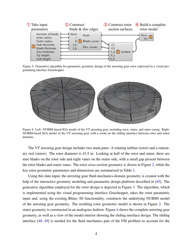
Figure 3: Generative algorithm for parametric geometry design of the arresting gear rotor expressed in a visual pro-gramming interface Grasshopper.

Figure 4: Left: NURBS-based IGA model of the VT arresting gear, including rotor, stator, and outer casing. Right:NURBS-based IGA model of the VT arresting gear with a zoom on the sliding interface between rotor and statordomains.

The VT arresting gear design includes two main parts: A rotating turbine (rotor) and a station-ary reel (stator). The rotor diameter is 43.5 in. Looking at half of the rotor and stator, there arenine blades on the rotor side and eight vanes on the stator side, with a small gap present betweenthe rotor blades and stator vanes. The rotor cross-section geometry is shown in Figure 2, while thekey rotor geometric parameters and dimensions are summarized in Table 1.

Using this data input, the arresting gear fluid-mechanics-domain geometry is created with thehelp of the interactive geometry modeling and parametric design platform described in [45]. Thegenerative algorithm employed for the rotor design is depicted in Figure 3. The algorithm, whichis implemented using the visual programming interface Grasshopper, takes the rotor parametricinput and, using the existing Rhino 3D functionality, constructs the underlying NURBS modelof the arresting gear geometry. The resulting rotor geometric model is shown in Figure 2. Thestator geometry is constructed in an analogous fashion. Figure 4 shows the complete arresting geargeometry, as well as a view of the model interior showing the sliding interface design. The slidinginterface [48, 49] is needed for the fluid mechanics part of the FSI problem to account for the

4

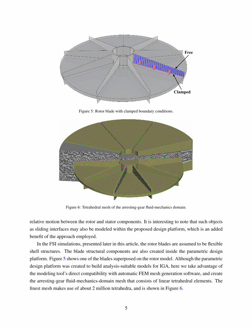
Free

Clamped

Figure 5: Rotor blade with clamped boundary conditions.

Figure 6: Tetrahedral mesh of the arresting-gear fluid-mechanics domain.

relative motion between the rotor and stator components. It is interesting to note that such objectsas sliding interfaces may also be modeled within the proposed design platform, which is an addedbenefit of the approach employed.

In the FSI simulations, presented later in this article, the rotor blades are assumed to be flexibleshell structures. The blade structural components are also created inside the parametric designplatform. Figure 5 shows one of the blades superposed on the rotor model. Although the parametricdesign platform was created to build analysis-suitable models for IGA, here we take advantage ofthe modeling tool’s direct compatibility with automatic FEM mesh generation software, and createthe arresting-gear fluid-mechanics-domain mesh that consists of linear tetrahedral elements. Thefinest mesh makes use of about 2 million tetrahedra, and is shown in Figure 6.

5

3. Governing Equations and Numerical Methods

The hydrodynamics of the arresting gear is governed by the Navier–Stokes equations of in-compressible flows, which are posed on a moving spatial domain and written in the ArbitraryLagrangian–Eulerian (ALE) frame [50] as follows:

ρ1

(∂u∂t

∣∣∣∣∣x

+ (u − u) · ∇∇∇u − f1

)−∇∇∇ ·σσσ1 = 0, (1)

∇∇∇ · u = 0. (2)

Here ρ1 is the fluid density, u is the velocity, f1 is the body force per unit mass, and u is the velocityof the fluid mechanics domain. The Cauchy stress, σσσ1, is given by

σσσ1 (u, p) = −pI + 2µε (u) , (3)

where p is the pressure, I is the identity tensor, µ is the dynamic viscosity, and ε (u) is the strain-ratetensor defined as

ε (u) =∇∇∇u +∇∇∇uT

2. (4)

The time derivative in Eq. (1) is taken with respect to the fixed referential-domain coordinates x.All space derivatives are taken with respect to spatial coordinates of the current configuration x.

The governing equations of structural mechanics are written in the Lagrangian frame [51] andconsist of the local balance of linear momentum:

ρ2

(d2ydt2 − f2

)−∇∇∇ ·σσσ2 = 0. (5)

Here ρ2 is the structural mass density, f2 is the body force per unit mass, σσσ2 is the Cauchy stress,and y is the unknown structural displacement. The time derivative in Eq. (5) is taken with respectto the fixed material coordinates of the structure reference configuration.

Compatibility of the kinematics and tractions is enforced at the fluid–structure interface,namely,

u −dydt

= 0, (6)

σσσ1n1 +σσσ2n2 = 0, (7)

where n1 and n2 are the unit outward normal vectors to the fluid and structural mechanics domains,respectively.

6

To discretize the arresting-gear hydrodynamics, the ALE–VMS method [52, 53] and weaklyenforced essential boundary conditions [54–56] are employed. The former is an extensionof the residual-based variational multiscale (RBVMS) large eddy simulation (LES) turbulencemodel [57] to moving domains using the ALE technique, while the latter acts as a “near-wallmodel” in that it relaxes boundary-layer resolution requirements to achieve good accuracy of fluidsolution and loads prediction on meshes without excessive boundary-layer refinement [58–63].

In the arresting gear design the stator is located in close proximity of the rotor, leaving onlya small gap as the rotor blades pass the stator vanes during the device operation. To capturethe complex dynamics of arresting-gear rotor-stator interaction, the sliding-interface techniquefrom [48, 49] is employed. We note that a similar method, called the slip-interface technique,was proposed more recently in the context of space–time FEM in [64], as an alternative to otherspace-time methods [65–70] developed to address this class of computational challenges.

The structural mechanics of rotor blades (the stator vanes are assumed to be rigid) is modeledusing Kirchhoff–Love shells [71, 72]. These are discretized using IGA based on NURBS [38, 39]and make use of only displacement degrees of freedom. Using rotation-free IGA shells to modelthe blades presents a good combination of efficiency, since no rotational degrees-of-freedom areemployed, accuracy, since NURBS are a higher-order accurate discretization technique [73], androbustness.

The coupled FSI problem is formulated using an augmented Lagrangian approach for FSI,which was originally proposed in [35] to handle boundary-fitted mesh computations with non-matching fluid–structure interface discretizations. The key feature of the method is formal elimi-nation of the Lagrange multiplier variable, which results in weak enforcement of the fluid–structureinterface compatibility conditions using only primal variables (i.e., fluid velocity and pressure, andstructure displacement), and, as a consequence, leads to increased efficiency compared to classicalLagrange-multiplier-based methods.

To accommodate the global rotor motion with superposed local blade elastic deformation, andto maintain a moving-mesh discretization, the fluid domain mesh is updated as follows. While atthe fluid–structure interface the fluid mechanics mesh follows the motion of the blades, the outerboundaries of the rotor subdomain are restricted to only undergo rigid rotation. This choice ofdomain motion preserves the geometry of the sliding interface. The rest of the mesh motion isobtained by solving the equations of elastostatics with Jacobian-based stiffening [4, 74–78].

The generalized-α method [79–81] is employed to advance to FSI equations in time, whileblock-iterative coupling strategy [2–4, 32] is used to solve the coupled FSI system at each timestep.

For a comprehensive discussion of numerical discretization techniques, coupling strategies,and application to a large class of problems in engineering we refer the reader to a recent book on

7

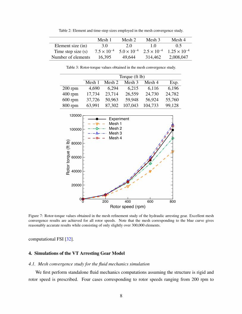
Table 2: Element and time-step sizes employed in the mesh convergence study.

Mesh 1 Mesh 2 Mesh 3 Mesh 4Element size (in) 3.0 2.0 1.0 0.5Time step size (s) 7.5 × 10−4 5.0 × 10−4 2.5 × 10−4 1.25 × 10−4

Number of elements 16,395 49,644 314,462 2,008,047

Table 3: Rotor-torque values obtained in the mesh convergence study.

Torque (ft lb)Mesh 1 Mesh 2 Mesh 3 Mesh 4 Exp.

200 rpm 4,690 6,294 6,215 6,116 6,196400 rpm 17,734 23,714 26,559 24,730 24,782600 rpm 37,726 50,963 59,948 56,924 55,760800 rpm 63,991 87,302 107,043 104,733 99,128

Rotor speed (rpm)

Roto

r tor

que

(ft lb

)

0 200 400 600 8000

20000

40000

60000

80000

100000

120000ExperimentMesh 1Mesh 2Mesh 3Mesh 4

Figure 7: Rotor-torque values obtained in the mesh refinement study of the hydraulic arresting gear. Excellent meshconvergence results are achieved for all rotor speeds. Note that the mesh corresponding to the blue curve givesreasonably accurate results while consisting of only slightly over 300,000 elements.

computational FSI [32].

4. Simulations of the VT Arresting Gear Model

4.1. Mesh convergence study for the fluid mechanics simulation

We first perform standalone fluid mechanics computations assuming the structure is rigid androtor speed is prescribed. Four cases corresponding to rotor speeds ranging from 200 rpm to

8

0 0.05 0.1 0.15 0.2 0.250

200

400

600

800An

gula

r acc

eler

atio

n (ra

d/s2 )

Time (s)

0

20

40

60

80

100

Time (s)

Rot

or s

peed

(rad

/s)

0 0.05 0.1 0.15 0.2 0.250

200

400

600

800

1000

Rot

or s

peed

(rpm

)

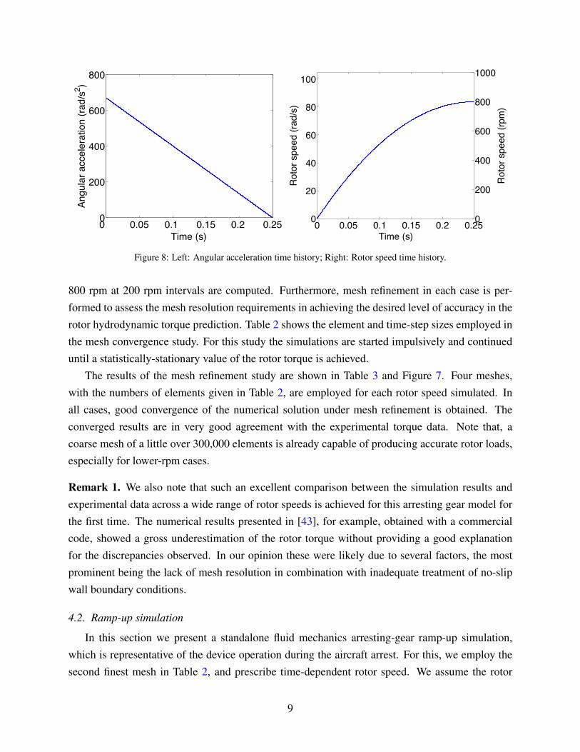
Figure 8: Left: Angular acceleration time history; Right: Rotor speed time history.

800 rpm at 200 rpm intervals are computed. Furthermore, mesh refinement in each case is per-formed to assess the mesh resolution requirements in achieving the desired level of accuracy in therotor hydrodynamic torque prediction. Table 2 shows the element and time-step sizes employed inthe mesh convergence study. For this study the simulations are started impulsively and continueduntil a statistically-stationary value of the rotor torque is achieved.

The results of the mesh refinement study are shown in Table 3 and Figure 7. Four meshes,with the numbers of elements given in Table 2, are employed for each rotor speed simulated. Inall cases, good convergence of the numerical solution under mesh refinement is obtained. Theconverged results are in very good agreement with the experimental torque data. Note that, acoarse mesh of a little over 300,000 elements is already capable of producing accurate rotor loads,especially for lower-rpm cases.

Remark 1. We also note that such an excellent comparison between the simulation results andexperimental data across a wide range of rotor speeds is achieved for this arresting gear model forthe first time. The numerical results presented in [43], for example, obtained with a commercialcode, showed a gross underestimation of the rotor torque without providing a good explanationfor the discrepancies observed. In our opinion these were likely due to several factors, the mostprominent being the lack of mesh resolution in combination with inadequate treatment of no-slipwall boundary conditions.

4.2. Ramp-up simulation

In this section we present a standalone fluid mechanics arresting-gear ramp-up simulation,which is representative of the device operation during the aircraft arrest. For this, we employ thesecond finest mesh in Table 2, and prescribe time-dependent rotor speed. We assume the rotor

9

0 0.5 1 1.5 20

2

4

6

8

10

12

14x 104

Time (s)

Rot

or to

rque

(ft l

b)

10.79.9

CFD simulationAveraged CFD torqueExperiment

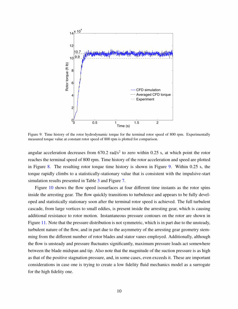
Figure 9: Time history of the rotor hydrodynamic torque for the terminal rotor speed of 800 rpm. Experimentallymeasured torque value at constant rotor speed of 800 rpm is plotted for comparison.

angular acceleration decreases from 670.2 rad/s2 to zero within 0.25 s, at which point the rotorreaches the terminal speed of 800 rpm. Time history of the rotor acceleration and speed are plottedin Figure 8. The resulting rotor torque time history is shown in Figure 9. Within 0.25 s, thetorque rapidly climbs to a statistically-stationary value that is consistent with the impulsive-startsimulation results presented in Table 3 and Figure 7.

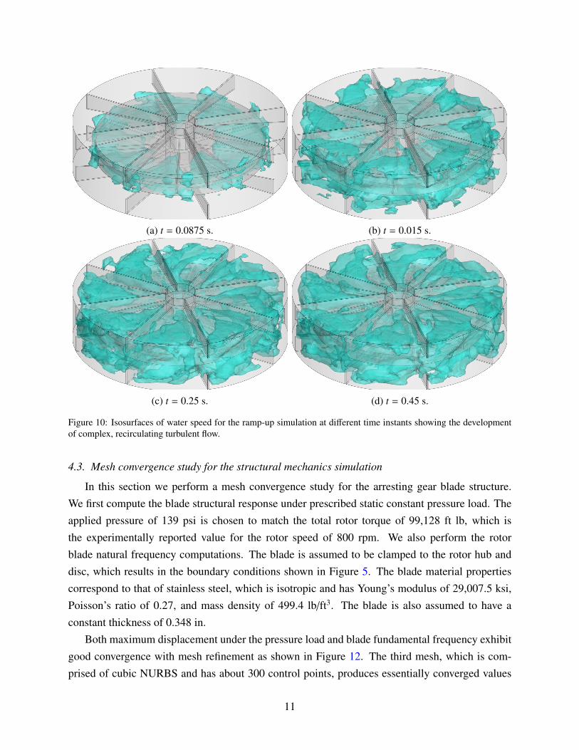
Figure 10 shows the flow speed isosurfaces at four different time instants as the rotor spinsinside the arresting gear. The flow quickly transitions to turbulence and appears to be fully devel-oped and statistically stationary soon after the terminal rotor speed is achieved. The full turbulentcascade, from large vortices to small eddies, is present inside the arresting gear, which is causingadditional resistance to rotor motion. Instantaneous pressure contours on the rotor are shown inFigure 11. Note that the pressure distribution is not symmetric, which is in part due to the unsteady,turbulent nature of the flow, and in part due to the asymmetry of the arresting gear geometry stem-ming from the different number of rotor blades and stator vanes employed. Additionally, althoughthe flow is unsteady and pressure fluctuates significantly, maximum pressure loads act somewherebetween the blade midspan and tip. Also note that the magnitude of the suction pressure is as highas that of the positive stagnation pressure, and, in some cases, even exceeds it. These are importantconsiderations in case one is trying to create a low fidelity fluid mechanics model as a surrogatefor the high fidelity one.

10

(a) t = 0.0875 s. (b) t = 0.015 s.

(c) t = 0.25 s. (d) t = 0.45 s.

Figure 10: Isosurfaces of water speed for the ramp-up simulation at different time instants showing the developmentof complex, recirculating turbulent flow.

4.3. Mesh convergence study for the structural mechanics simulation

In this section we perform a mesh convergence study for the arresting gear blade structure.We first compute the blade structural response under prescribed static constant pressure load. Theapplied pressure of 139 psi is chosen to match the total rotor torque of 99,128 ft lb, which isthe experimentally reported value for the rotor speed of 800 rpm. We also perform the rotorblade natural frequency computations. The blade is assumed to be clamped to the rotor hub anddisc, which results in the boundary conditions shown in Figure 5. The blade material propertiescorrespond to that of stainless steel, which is isotropic and has Young’s modulus of 29,007.5 ksi,Poisson’s ratio of 0.27, and mass density of 499.4 lb/ft3. The blade is also assumed to have aconstant thickness of 0.348 in.

Both maximum displacement under the pressure load and blade fundamental frequency exhibitgood convergence with mesh refinement as shown in Figure 12. The third mesh, which is com-prised of cubic NURBS and has about 300 control points, produces essentially converged values

11

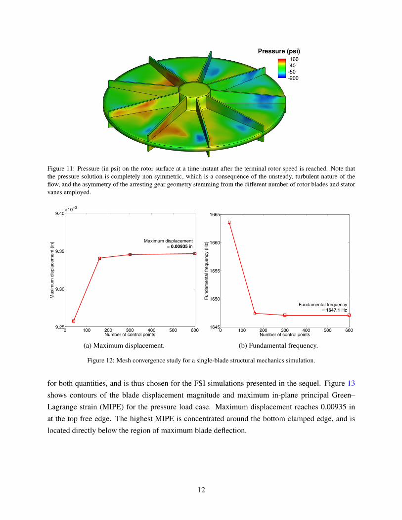
Figure 11: Pressure (in psi) on the rotor surface at a time instant after the terminal rotor speed is reached. Note thatthe pressure solution is completely non symmetric, which is a consequence of the unsteady, turbulent nature of theflow, and the asymmetry of the arresting gear geometry stemming from the different number of rotor blades and statorvanes employed.

0 100 200 300 400 500 6009.25

9.30

9.35

9.40

Number of control points

Max

imum

dis

plac

emen

t (in

)

×10−3

Maximum displacement= 0.00935 in

(a) Maximum displacement.

0 100 200 300 400 500 6001645

1650

1655

1660

1665

Number of control points

Fund

amen

tal f

requ

ency

(Hz)

Fundamental frequency= 1647.1 Hz

(b) Fundamental frequency.

Figure 12: Mesh convergence study for a single-blade structural mechanics simulation.

for both quantities, and is thus chosen for the FSI simulations presented in the sequel. Figure 13shows contours of the blade displacement magnitude and maximum in-plane principal Green–Lagrange strain (MIPE) for the pressure load case. Maximum displacement reaches 0.00935 inat the top free edge. The highest MIPE is concentrated around the bottom clamped edge, and islocated directly below the region of maximum blade deflection.

12

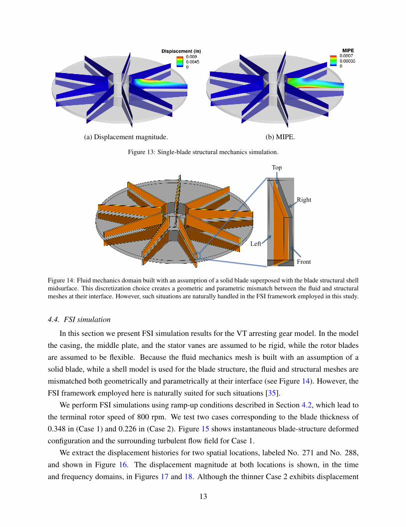
(a) Displacement magnitude. (b) MIPE.

Figure 13: Single-blade structural mechanics simulation.

Top

Left

Right

Front

Figure 14: Fluid mechanics domain built with an assumption of a solid blade superposed with the blade structural shellmidsurface. This discretization choice creates a geometric and parametric mismatch between the fluid and structuralmeshes at their interface. However, such situations are naturally handled in the FSI framework employed in this study.

4.4. FSI simulation

In this section we present FSI simulation results for the VT arresting gear model. In the modelthe casing, the middle plate, and the stator vanes are assumed to be rigid, while the rotor bladesare assumed to be flexible. Because the fluid mechanics mesh is built with an assumption of asolid blade, while a shell model is used for the blade structure, the fluid and structural meshes aremismatched both geometrically and parametrically at their interface (see Figure 14). However, theFSI framework employed here is naturally suited for such situations [35].

We perform FSI simulations using ramp-up conditions described in Section 4.2, which lead tothe terminal rotor speed of 800 rpm. We test two cases corresponding to the blade thickness of0.348 in (Case 1) and 0.226 in (Case 2). Figure 15 shows instantaneous blade-structure deformedconfiguration and the surrounding turbulent flow field for Case 1.

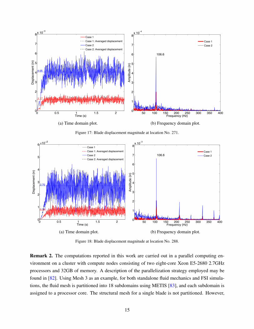
We extract the displacement histories for two spatial locations, labeled No. 271 and No. 288,and shown in Figure 16. The displacement magnitude at both locations is shown, in the timeand frequency domains, in Figures 17 and 18. Although the thinner Case 2 exhibits displacement

13

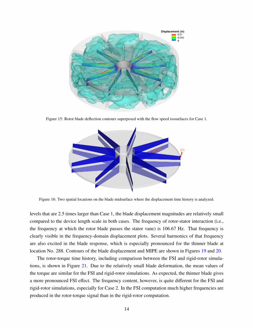
Figure 15: Rotor blade deflection contours superposed with the flow speed isosurfaces for Case 1.

271$288$

Figure 16: Two spatial locations on the blade midsurface where the displacement time history is analyzed.

levels that are 2.5 times larger than Case 1, the blade displacement magnitudes are relatively smallcompared to the device length scale in both cases. The frequency of rotor-stator interaction (i.e.,the frequency at which the rotor blade passes the stator vane) is 106.67 Hz. That frequency isclearly visible in the frequency-domain displacement plots. Several harmonics of that frequencyare also excited in the blade response, which is especially pronounced for the thinner blade atlocation No. 288. Contours of the blade displacement and MIPE are shown in Figures 19 and 20.

The rotor-torque time history, including comparison between the FSI and rigid-rotor simula-tions, is shown in Figure 21. Due to the relatively small blade deformation, the mean values ofthe torque are similar for the FSI and rigid-rotor simulations. As expected, the thinner blade givesa more pronounced FSI effect. The frequency content, however, is quite different for the FSI andrigid-rotor simulations, especially for Case 2. In the FSI computation much higher frequencies areproduced in the rotor-torque signal than in the rigid-rotor computation.

14

0 0.5 1 1.5 20

1

2

3

4

5

6

7

8x 10−3

Time (s)

Dis

plac

emen

t (in

)

1.17

4.05

Case 1Case 1: Averaged displacementCase 2Case 2: Averaged displacement

(a) Time domain plot.

50 100 150 200 250 300 350 4000

1

2

3

4

5

6

7

8x 10−4

Frequency (Hz)

Ampl

itude

(in)

106.6

Case 1Case 2

(b) Frequency domain plot.

Figure 17: Blade displacement magnitude at location No. 271.

0 0.5 1 1.5 2 0

1

2

3

4

5

6

Time (s)

Dis

plac

emen

t (in

)

×10−2

0.74

2.70

Case 1Case 1: Averaged displacementCase 2Case 2: Averaged displacement

(a) Time domain plot.

50 100 150 200 250 300 350 4000

1

2

3

4

5

6

7

8x 10−3

Frequency (Hz)

Ampl

itude

(in)

106.6

Case 1Case 2

(b) Frequency domain plot.

Figure 18: Blade displacement magnitude at location No. 288.

Remark 2. The computations reported in this work are carried out in a parallel computing en-vironment on a cluster with compute nodes consisting of two eight-core Xeon E5-2680 2.7GHzprocessors and 32GB of memory. A description of the parallelization strategy employed may befound in [82]. Using Mesh 3 as an example, for both standalone fluid mechanics and FSI simula-tions, the fluid mesh is partitioned into 18 subdomains using METIS [83], and each subdomain isassigned to a processor core. The structural mesh for a single blade is not partitioned. However,

15

(a) Case 1. (b) Case 2.

Figure 19: Contours of blade displacement magnitude. (A scaling factor of 100 is applied to the displacement forvisualization.)

(a) Case 1. (b) Case 2.

Figure 20: Contours of MIPE. (A scaling factor of 100 is applied to the displacement for visualization.)

0.8 0.85 0.9 0.95 19.5

10.0

10.5

11.0

11.5

Time (s)

Rot

or to

rque

(ft l

b)

×104

FSI torqueAveraged FSI torqueCFD torqueAveraged CFD torque

(a) Case 1.

0.8 0.85 0.9 0.95 19.5

10.0

10.5

11.0

11.5

Time (s)

Rot

or to

rque

(ft l

b)

×104

FSI torqueAveraged FSI torqueCFD torqueAveraged CFD torque

(b) Case 2.

Figure 21: Rotor-torque time history for FSI and rigid-rotor simulations, the latter denoted by “CFD torque”.

16

each blade is assigned to a different processor core to improve overall efficiency. For the simu-lations in Figure 21b, we use three Newton iterations per time step, with 100 to 125 diagonally-preconditioned-GMRES iterations. The standalone fluid mechanics and FSI computations take 1.8and 2.7 hours, respectively, to run 500 time steps.

5. Conclusion

In this work we developed a “pipeline” for geometry modeling and predictive FSI simulation ofhydraulic arresting gears at full scale. A parametric modeling platform recently proposed in [45]was adapted to generate analysis-suitable IGA models for this complex system. The FSI simula-tions were carried out for the VT arresting gear model using a combination of IGA to discretize thestructural mechanics part, and FEM to discretize the hydrodynamics part of the coupled problem.Careful mesh convergence studies were performed for standalone fluid and structural analyses ofthe VT arresting gear model. One of the findings of the mesh convergence study was that despitethe underlying complexity of the turbulent flow inside the arresting gear, a relatively modest size offluid mechanics mesh was needed to accurately capture the rotor hydrodynamic loads. This goodaccuracy is attributable to the use of the ALE-VMS technique with weakly enforced boundaryconditions as the underlying numerical methodology. The FSI simulations produced rotor bladedisplacements that are relatively low compared to the device length scale. However, the vibra-tional response predicted the presence of multiple highly pronounced frequencies, especially forthe thinner blade design. This finding is intriguing and needs to be investigated in the future work.

Acknowledgements

This work was supported by NAVAIR, Program Manager Dr. Nam Phan, and ARO grant No.W911NF-14-1-0296, Program Manager Dr. Joseph Myers. This support is gratefully acknowl-edged.

References

[1] T. E. Tezduyar, S. Sathe, R. Keedy, and K. Stein. Space–time techniques for finite elementcomputation of flows with moving boundaries and interfaces. In S. Gallegos, I. Herrera,S. Botello, F. Zarate, and G. Ayala, editors, Proceedings of the III International Congress

on Numerical Methods in Engineering and Applied Science. CD-ROM, Monterrey, Mexico,2004.

[2] T. E. Tezduyar, S. Sathe, R. Keedy, and K. Stein. Space–time finite element techniques forcomputation of fluid–structure interactions. Computer Methods in Applied Mechanics and

Engineering, 195:2002–2027, 2006.

17

[3] T. E. Tezduyar, S. Sathe, and K. Stein. Solution techniques for the fully-discretized equationsin computation of fluid–structure interactions with the space–time formulations. Computer

Methods in Applied Mechanics and Engineering, 195:5743–5753, 2006.

[4] T. E. Tezduyar and S. Sathe. Modeling of fluid–structure interactions with the space–timefinite elements: Solution techniques. International Journal for Numerical Methods in Fluids,54:855–900, 2007.

[5] K. Takizawa, S. Wright, C. Moorman, and T. E. Tezduyar. Fluid–structure interaction mod-eling of parachute clusters. International Journal for Numerical Methods in Fluids, 65:286–307, 2011.

[6] K. Takizawa, T. Spielman, and T. E. Tezduyar. Space–time FSI modeling and dynamicalanalysis of spacecraft parachutes and parachute clusters. Computational Mechanics, 48:345–364, 2011.

[7] K. Takizawa and T. E. Tezduyar. Computational methods for parachute fluid–structure inter-actions. Archives of Computational Methods in Engineering, 19:125–169, 2012.

[8] K. Takizawa, T. E. Tezduyar, J. Boben, N. Kostov, C. Boswell, and A. Buscher. Fluid–structure interaction modeling of clusters of spacecraft parachutes with modified geometricporosity. Computational Mechanics, 52:1351–1364, 2013.

[9] K. Takizawa, D. Montes, M. Fritze, S. McIntyre, J. Boben, and T. E. Tezduyar. Methods forFSI modeling of spacecraft parachute dynamics and cover separation. Mathematical Models

and Methods in Applied Sciences, 23:307–338, 2013.

[10] K. Takizawa, T. E. Tezduyar, C. Boswell, R. Kolesar, and K. Montel. FSI modeling of thereefed stages and disreefing of the Orion spacecraft parachutes. Computational Mechanics,54:1203–1220, 2014.

[11] K. Takizawa, T. E. Tezduyar, R. Kolesar, C. Boswell, T. Kanai, and K. Montel. Multiscalemethods for gore curvature calculations from FSI modeling of spacecraft parachutes. Com-

putational Mechanics, 54:1461–1476, 2014.

[12] K. Takizawa, T. E. Tezduyar, C. Boswell, Y. Tsutsui, and K. Montel. Special methods foraerodynamic-moment calculations from parachute FSI modeling. Computational Mechanics,55:1059–1069, 2015.

[13] K. Takizawa, T. E. Tezduyar, and R. Kolesar. FSI modeling of the Orion spacecraft drogueparachutes. Computational Mechanics, 55:1167–1179, 2015.

18

[14] Y. Bazilevs, M.-C. Hsu, D. Benson, S. Sankaran, and A. Marsden. Computational fluid–structure interaction: Methods and application to a total cavopulmonary connection. Compu-

tational Mechanics, 45:77–89, 2009.

[15] Y. Bazilevs, M.-C. Hsu, Y. Zhang, W. Wang, X. Liang, T. Kvamsdal, R. Brekken, and J. Isak-sen. A fully-coupled fluid–structure interaction simulation of cerebral aneurysms. Computa-

tional Mechanics, 46:3–16, 2010.

[16] Y. Bazilevs, M.-C. Hsu, Y. Zhang, W. Wang, T. Kvamsdal, S. Hentschel, and J. Isaksen.Computational fluid–structure interaction: Methods and application to cerebral aneurysms.Biomechanics and Modeling in Mechanobiology, 9:481–498, 2010.

[17] M.-C. Hsu and Y. Bazilevs. Blood vessel tissue prestress modeling for vascular fluid–structure interaction simulations. Finite Elements in Analysis and Design, 47:593–599, 2011.

[18] C. C. Long, M.-C. Hsu, Y. Bazilevs, J. A. Feinstein, and A. L. Marsden. Fluid–structureinteraction simulations of the Fontan procedure using variable wall properties. International

Journal for Numerical Methods in Biomedical Engineering, 28:512–527, 2012.

[19] K. Takizawa, K. Schjodt, A. Puntel, N. Kostov, and T. E. Tezduyar. Patient-specific com-putational analysis of the influence of a stent on the unsteady flow in cerebral aneurysms.Computational Mechanics, 51:1061–1073, 2013.

[20] K. Takizawa, H. Takagi, T. E. Tezduyar, and R. Torii. Estimation of element-based zero-stressstate for arterial FSI computations. Computational Mechanics, 54:895–910, 2014.

[21] K. Takizawa, T. E. Tezduyar, A. Buscher, and S. Asada. Space-time interface-tracking withtopology change (ST-TC). Computational Mechanics, 54:955–971, 2014.

[22] K. Takizawa. Computational engineering analysis with the new-generation space–time meth-ods. Computational Mechanics, 54:193–211, 2014.

[23] K. Takizawa, Y. Bazilevs, T. E. Tezduyar, C. C. Long, A. L. Marsden, and K. Schjodt. STand ALE-VMS methods for patient-specific cardiovascular fluid mechanics modeling. Math-

ematical Models and Methods in Applied Sciences, 24:2437–2486, 2014.

[24] K. Takizawa, T. E. Tezduyar, A Buscher, and S. Asada. Space–time fluid mechanics compu-tation of heart valve models. Computational Mechanics, 54:973–986, 2014.

[25] K. Takizawa, R. Torii, H. Takagi, T. E. Tezduyar, and X. Y. Xu. Coronary arterial dynam-ics computation with medical-image-based time-dependent anatomical models and element-based zero-stress state estimates. Computational Mechanics, 54:1047–1053, 2014.

19

[26] C. C. Long, A. L. Marsden, and Y. Bazilevs. Fluid–structure interaction simulation of pul-satile ventricular assist devices. Computational Mechanics, 52:971–981, 2013.

[27] C. C. Long, M. Esmaily-Moghadam, A. L. Marsden, and Y. Bazilevs. Computation of resi-dence time in the simulation of pulsatile ventricular assist devices. Computational Mechanics,54:911–919, 2014.

[28] C. C. Long, A. L. Marsden, and Y. Bazilevs. Shape optimization of pulsatile ventricularassist devices using FSI to minimize thrombotic risk. Computational Mechanics, 54:921–932, 2014.

[29] M.-C. Hsu, D. Kamensky, Y. Bazilevs, M. S. Sacks, and T. J. R. Hughes. Fluid–structureinteraction analysis of bioprosthetic heart valves: significance of arterial wall deformation.Computational Mechanics, 54:1055–1071, 2014.

[30] M.-C. Hsu, D. Kamensky, F. Xu, J. Kiendl, C. Wang, M. C. H. Wu, J. Mineroff, A. Re-ali, Y. Bazilevs, and M. S. Sacks. Dynamic and fluid–structure interaction simulations ofbioprosthetic heart valves using parametric design with T-splines and Fung-type materialmodels. Computational Mechanics, 55:1211–1225, 2015.

[31] D. Kamensky, M.-C. Hsu, D. Schillinger, J. A. Evans, A. Aggarwal, Y. Bazilevs, M. S. Sacks,and T. J. R. Hughes. An immersogeometric variational framework for fluid-structure inter-action: Application to bioprosthetic heart valves. Computer Methods in Applied Mechanics

and Engineering, 284:1005–1053, 2015.

[32] Y. Bazilevs, K. Takizawa, and T. E. Tezduyar. Computational Fluid–Structure Interaction:

Methods and Applications. Wiley, 2013.

[33] Y. Bazilevs, K. Takizawa, and T. E. Tezduyar. Challenges and directions in computationalfluid–structure interaction. Mathematical Models and Methods in Applied Sciences, 23:215–221, 2013.

[34] K. Takizawa, D. Montes, S. McIntyre, and T. E. Tezduyar. Space–time VMS methods formodeling of incompressible flows at high Reynolds numbers. Mathematical Models and

Methods in Applied Sciences, 23:223–248, 2013.

[35] Y. Bazilevs, M.-C. Hsu, and M. A. Scott. Isogeometric fluid–structure interaction analysiswith emphasis on non-matching discretizations, and with application to wind turbines. Com-

puter Methods in Applied Mechanics and Engineering, 249-252:28–41, 2012.

20

[36] K. Takizawa and T. E. Tezduyar. Space–time computation techniques with continuous repre-sentation in time (ST-C). Computational Mechanics, 53:91–99, 2014.

[37] K. Takizawa, T. E. Tezduyar, and T. Kuraishi. Multiscale ST methods for thermo-fluid analy-sis of a ground vehicle and its tires. Mathematical Models and Methods in Applied Sciences,25:2227–2255, 2015.

[38] T. J. R. Hughes, J. A. Cottrell, and Y. Bazilevs. Isogeometric analysis: CAD, finite elements,NURBS, exact geometry, and mesh refinement. Computer Methods in Applied Mechanics

and Engineering, 194:4135–4195, 2005.

[39] J. A. Cottrell, T. J. R. Hughes, and Y. Bazilevs. Isogeometric Analysis: Toward Integration

of CAD and FEA. Wiley, Chichester, 2009.

[40] L. Piegl and W. Tiller. The NURBS Book (Monographs in Visual Communication), 2nd ed.

Springer-Verlag, New York, 1997.

[41] Autodesk T-Splines Plug-in for Rhino. http://www.tsplines.com/products/tsplines-for-rhino.html. 2015.

[42] M. A. Scott, T. J. R. Hughes, T. W. Sederberg, and M. T. Sederberg. An integrated approachto engineering design and analysis using the Autodesk T-spline plugin for Rhino3d. ICESREPORT 14-33, The Institute for Computational Engineering and Sciences, The Universityof Texas at Austin, September 2014, 2014.

[43] Y.-T. Chiu. Computational fluid dynamics simulations of hydraulic energy absorber. Master’sthesis, Virginia Polytechnic Institute and State University, 1999.

[44] R. V. Parker. Arrestment considerations for the space shuttle. In The Space Congress Pro-

ceedings, Wilmington, Delaware, 1971.

[45] M.-C. Hsu, C. Wang, A. G. Herrema, D. Schillinger, A. Ghoshal, and Y. Bazilevs. An interac-tive geometry modeling and parametric design platform for isogeometric analysis. Computers

& Mathematics with Applications, 2015. http://dx.doi.org/10.1016/j.camwa.2015.04.002.

[46] Rhinoceros. http://www.rhino3d.com/. 2015.

[47] Grasshopper. http://www.grasshopper3d.com/. 2015.

[48] Y. Bazilevs and T. J. R. Hughes. NURBS-based isogeometric analysis for the computation offlows about rotating components. Computational Mechanics, 43:143–150, 2008.

21

[49] M.-C. Hsu and Y. Bazilevs. Fluid–structure interaction modeling of wind turbines: simulatingthe full machine. Computational Mechanics, 50:821–833, 2012.

[50] T. J. R. Hughes, W. K. Liu, and T. K. Zimmermann. Lagrangian–Eulerian finite elementformulation for incompressible viscous flows. Computer Methods in Applied Mechanics and

Engineering, 29:329–349, 1981.

[51] T. Belytschko, W. K. Liu, and B. Moran. Nonlinear Finite Elements for Continua and Struc-

tures. Wiley, 2000.

[52] K. Takizawa, Y. Bazilevs, and T. E. Tezduyar. Space–time and ALE-VMS techniques forpatient-specific cardiovascular fluid–structure interaction modeling. Archives of Computa-

tional Methods in Engineering, 19:171–225, 2012.

[53] Y. Bazilevs, M.-C. Hsu, K. Takizawa, and T. E. Tezduyar. ALE-VMS and ST-VMS methodsfor computer modeling of wind-turbine rotor aerodynamics and fluid–structure interaction.Mathematical Models and Methods in Applied Sciences, 22(supp02):1230002, 2012.

[54] Y. Bazilevs and T. J. R. Hughes. Weak imposition of Dirichlet boundary conditions in fluidmechanics. Computers and Fluids, 36:12–26, 2007.

[55] Y. Bazilevs, C. Michler, V. M. Calo, and T. J. R. Hughes. Weak Dirichlet boundary conditionsfor wall-bounded turbulent flows. Computer Methods in Applied Mechanics and Engineering,196:4853–4862, 2007.

[56] Y. Bazilevs, C. Michler, V. M. Calo, and T. J. R. Hughes. Isogeometric variational multiscalemodeling of wall-bounded turbulent flows with weakly enforced boundary conditions on un-stretched meshes. Computer Methods in Applied Mechanics and Engineering, 199:780–790,2010.

[57] Y. Bazilevs, V. M. Calo, J. A. Cottrel, T. J. R. Hughes, A. Reali, and G. Scovazzi. Variationalmultiscale residual-based turbulence modeling for large eddy simulation of incompressibleflows. Computer Methods in Applied Mechanics and Engineering, 197:173–201, 2007.

[58] I. Akkerman, Y. Bazilevs, C. E. Kees, and M. W. Farthing. Isogeometric analysis of free-surface flow. Journal of Computational Physics, 230:4137–4152, 2011.

[59] C. E. Kees, I. Akkerman, M. W. Farthing, and Y. Bazilevs. A conservative level set methodsuitable for variable-order approximations and unstructured meshes. Journal of Computa-

tional Physics, 230:4536–4558, 2011.

22

[60] I. Akkerman, Y. Bazilevs, D. J. Benson, M. W. Farthing, and C. E. Kees. Free-surface flowand fluid–object interaction modeling with emphasis on ship hydrodynamics. Journal of

Applied Mechanics, 79:010905, 2012.

[61] M.-C. Hsu, I. Akkerman, and Y. Bazilevs. Wind turbine aerodynamics using ALE–VMS:Validation and the role of weakly enforced boundary conditions. Computational Mechanics,50:499–511, 2012. doi:10.1007/s00466-012-0686-x.

[62] I. Akkerman, J. Dunaway, J. Kvandal, J. Spinks, and Y. Bazilevs. Toward free-surface mod-eling of planing vessels: simulation of the Fridsma hull using ALE-VMS. Computational

Mechanics, 50:719–727, 2012.

[63] M.-C. Hsu, I. Akkerman, and Y. Bazilevs. Finite element simulation of wind turbine aero-dynamics: Validation study using NREL Phase VI experiment. Wind Energy, 17:461–481,2014.

[64] K. Takizawa, T. E. Tezduyar, H. Mochizuki, H. Hattori, S. Mei, L. Pan, and K. Montel.Space–time VMS method for flow computations with slip interfaces (ST-SI). Mathematical

Models and Methods in Applied Sciences, 25:2377–2406, 2015.

[65] K. Takizawa, T. E. Tezduyar, S. McIntyre, N. Kostov, R. Kolesar, and C. Habluetzel. Space–time VMS computation of wind-turbine rotor and tower aerodynamics. Computational Me-

chanics, 53:1–15, 2014.

[66] K. Takizawa, T. E. Tezduyar, and N. Kostov. Sequentially-coupled space–time FSI analysisof bio-inspired flapping-wing aerodynamics of an MAV. Computational Mechanics, 54:213–233, 2014.

[67] K. Takizawa, Y. Bazilevs, T. E. Tezduyar, M.-C. Hsu, O. Øiseth, K. M. Mathisen, N. Kostov,and S. McIntyre. Engineering analysis and design with ALE-VMS and space–time methods.Archives of Computational Methods in Engineering, 21:481–508, 2014.

[68] Y. Bazilevs, K. Takizawa, T. E. Tezduyar, M.-C. Hsu, N. Kostov, and S. McIntyre. Aero-dynamic and FSI analysis of wind turbines with the ALE–VMS and ST–VMS methods.Archives of Computational Methods in Engineering, 21:359–398, 2014.

[69] K. Takizawa, T. E. Tezduyar, and A. Buscher. Space–time computational analysis of MAVflapping-wing aerodynamics with wing clapping. Computational Mechanics, 55:1131–1141,2015.

23

[70] Y. Bazilevs, K. Takizawa, and T. E. Tezduyar. New directions and challenging computationsin fluid dynamics modeling with stabilized and multiscale methods. Mathematical Models

and Methods in Applied Sciences, 25:2217–2226, 2015.

[71] J. Kiendl, K.-U. Bletzinger, J. Linhard, and R. Wuchner. Isogeometric shell analysis withKirchhoff–Love elements. Computer Methods in Applied Mechanics and Engineering,198:3902–3914, 2009.

[72] J. Kiendl, Y. Bazilevs, M.-C. Hsu, R. Wuchner, and K.-U. Bletzinger. The bending stripmethod for isogeometric analysis of Kirchhoff–Love shell structures comprised of multiplepatches. Computer Methods in Applied Mechanics and Engineering, 199:2403–2416, 2010.

[73] Y. Bazilevs, L. Beirao da Veiga, J. A. Cottrell, T. J. R. Hughes, and G. Sangalli. Isogeometricanalysis: Approximation, stability and error estimates for h-refined meshes. Mathematical

Models and Methods in Applied Sciences, 16:1031–1090, 2006.

[74] T. E. Tezduyar, M. Behr, S. Mittal, and A. A. Johnson. Computation of unsteady incom-pressible flows with the finite element methods – space–time formulations, iterative strate-gies and massively parallel implementations. In New Methods in Transient Analysis, PVP-Vol.246/AMD-Vol.143, pages 7–24, New York, 1992. ASME.

[75] T. Tezduyar, S. Aliabadi, M. Behr, A. Johnson, and S. Mittal. Parallel finite-element compu-tation of 3D flows. Computer, 26(10):27–36, 1993.

[76] A. A. Johnson and T. E. Tezduyar. Mesh update strategies in parallel finite element computa-tions of flow problems with moving boundaries and interfaces. Computer Methods in Applied

Mechanics and Engineering, 119:73–94, 1994.

[77] T. E. Tezduyar. Finite element methods for flow problems with moving boundaries and inter-faces. Archives of Computational Methods in Engineering, 8:83–130, 2001.

[78] K. Stein, T. Tezduyar, and R. Benney. Mesh moving techniques for fluid–structure interac-tions with large displacements. Journal of Applied Mechanics, 70:58–63, 2003.

[79] Y. Bazilevs, V. M. Calo, T. J. R. Hughes, and Y. Zhang. Isogeometric fluid–structure interac-tion: theory, algorithms, and computations. Computational Mechanics, 43:3–37, 2008.

[80] J. Chung and G. M. Hulbert. A time integration algorithm for structural dynamics withim-proved numerical dissipation: The generalized-α method. Journal of Applied Mechanics,60:371–75, 1993.

24

[81] K. E. Jansen, C. H. Whiting, and G. M. Hulbert. A generalized-α method for integrating thefiltered Navier-Stokes equations with a stabilized finite element method. Computer Methods

in Applied Mechanics and Engineering, 190:305–319, 2000.

[82] M.-C. Hsu, I. Akkerman, and Y. Bazilevs. High-performance computing of wind turbineaerodynamics using isogeometric analysis. Computers & Fluids, 49:93–100, 2011.

[83] G. Karypis and V. Kumar. A fast and high quality multilevel scheme for partitioning irregulargraphs. SIAM Journal on Scientific Computing, 20:359–392, 1999.

25