Modeling Monetary Policy Dynamics: A Comparison of Regime

Switching and Time Varying Parameter Approaches

Aeimit Lakdawala∗

Michigan State University

October 2015

Abstract

Structural VAR models have been widely used to model monetary policy dynamics. Typi-

cally, a choice is made between regime switching and time varying parameter models. In this

paper we use a canonical model of monetary policy and estimate both types of time variation

in monetary policy while also allowing for changing variances. The models are compared using

marginal likelihood and forecasting performance. We find that for both frameworks, the best-fit

model implies a specification with changes only in the variance of shocks and the implied model

dynamics are similar. However, researchers using a specification with only changes in monetary

policy coefficients would reach different conclusions about the dynamic behavior of monetary

policy.

JEL classification: C32, E52, E47.

Keywords: Structural VAR, monetary policy, regime switching, time varying parameter, model

comparison

∗Email: aeimit@msu.edu, Address: 486 W. Circle Drive, 110 Marshall-Adams Hall, East Lansing, MI 48824

1

1 Introduction

There is a large literature that studies changes in the behavior of monetary policy setting in

the post-war US data. The most common way to model monetary policy, both in structural macro

models and reduced form VAR models, is to use a Taylor-type interest rate rule. This is a simple

linear rule where the short term interest rate is adjusted in response to some measure of inflation

and economic activity. To allow for changes in the behavior of monetary policy, the parameters of

this simple rule are allowed to change over time. From a modeling perspective, the econometrician

has to specify some process for the time variation in the parameters. There are two common

approaches that have been used in the literature. The first one, known as the regime switching

(rs) approach, assumes that there are discrete changes in the parameters which are governed by a

Markov switching variable. This approach has been used in VAR analysis by Sims and Zha (2006)

and in structural DSGE models by Bianchi (2013) and Liu et al. (2011) among others. The other

approach, known as the time varying parameter (tvp) approach, assumes that there are gradual

changes in the parameters. The time variation is typically specified as an autoregressive process.

This has been used in VAR analysis by Cogley and Sargent (2005) and Primiceri (2005) and in

structural DSGE models by Fernandez-Villaverde et al. (2010). Sometimes, a theoretical model is

used to motivate the choice between the two frameworks, but more often the choice turns out to

be driven by convenience and tractability. In this paper we compare the two approaches using a

structural VAR model and explore the implications for monetary policy dynamics.

Specifically, we want to study whether the choice of one method over the other yields results

that lead to divergent answers to important questions related to monetary policy. First, there is a

debate in the literature regarding changes in the macroeconomy since the 1980s. Was there a change

in monetary policy or was it just a change in the volatility of shocks hitting the economy, or perhaps

both? One approach has been to estimate models with time variation allowed in both the monetary

policy parameters and the shock volatility parameters.1 Then some form of model comparison is

performed to identify the specification which best fits the data. In this paper we want to examine

1See Primiceri (2005) and Sargent et al. (2006) for examples that use tvp and Sims and Zha (2006) for a rsapproach.

2

whether using a tvp or rs approach gives rise to a different conclusion. Second, if there has been a

change in monetary policy, how does the choice of tvp vs. rs affect the characterization of historical

changes in monetary policy? For instance, was there a big change in the reaction of the Federal

Reserve to inflation when Paul Volcker was elected or was it gradual, beginning before the arrival

of Volcker? Another important question is whether Federal Reserve policy in the 1970s satisfied the

Taylor principle. Finally, how does this choice affect the evaluation of monetary policy’s effects on

the economy? A key component in this evaluation is the identification of monetary policy shocks

and we investigate whether the choice of rs vs. tvp matters for the series of identified monetary

shocks.

We consider a canonical three variable structural VAR with unemployment, inflation and

the fed funds rate.2 The VAR is identified using the recursive (also called triangular) identifying

restriction that is most common in the monetary policy literature. Under this assumption, both

inflation and unemployment react with a lag to changes in the fed funds rate while the fed funds rate

is allowed to react contemporaneously to inflation and unemployment. The equation corresponding

to the interest rate is interpreted as the monetary policy reaction function. Since the focus of the

paper is on monetary policy, the coefficients of only this equation are allowed to change over time,

either using a time varying parameter or regime switching framework. The variance of the shocks

are also allowed to change over time. The tvp specification is based on the framework of Primiceri

(2005) with the same prior specification.3 The rs specification is similar to the models in Sims et al.

(2008), with the main difference that we use fairly loose priors that do not put any restrictions on

the time variation. This is done to keep the priors in the rs setup comparable to the tvp setup. All

models are estimated using a Bayesian Markov Chain Monte Carlo algorithm.

The main results regarding the monetary policy questions are as follows. First, if a re-

searcher were to adhere to either the tvp or rs framework and consider the best fit model within

2Others have studied the question of time variation in monetary policy and shock variances in DSGE type models.Bianchi (2013) and Fernandez-Villaverde et al. (2010) allow time variation in coefficients of the Taylor rule while Liuet al. (2011) model time variation in the inflation target. We choose a VAR framework as it makes the comparisonbetween the rs and tvp frameworks more straightforward as compared to a DSGE type setting where the modelingof agents’ expectations, equilibrium definitions and model solution techniques are not agreed upon in the literature.

3The only difference is that in this paper time variation in the coefficients is only allowed in the monetary policyequation.

3

that framework, the specification with changes only in the variance would be picked for both the

rs and tvp specifications. Even though there are some differences in the dynamics of the estimated

changes in the variances, the monetary policy shocks identified are almost identical implying very

similar effects of monetary policy on the economy. Thus our results are consistent with the litera-

ture that finds that the data are more supportive of models in which the variance of shocks - rather

than monetary policy coefficients - have changed over time (see Primiceri (2005), Liu et al. (2011)

and Sims and Zha (2006)). But, as motivated in Benati and Surico (2009), it is also interesting

to look at a framework with just changes in the monetary policy coefficients. Here we find that

the dynamic patterns are different between the tvp and rs cases. Specifically, the changes in the

response to inflation are more gradual in the tvp case. Additionally, the Taylor principle is satisfied

for essentially the whole sample in the tvp vase. On the other hand, the rs specification implies

frequent changes in the 1970s between high response to inflation that satisfies the Taylor principle

and low responses that do not satisfy it. As a result the monetary policy shocks identified by the rs

regime are quite different (especially in the 1970s) from the tvp case, which has important reper-

cussions for the evaluation of monetary policy’s effect on the economy. Thus our results highlight

the fact that the choice of rs vs. tvp can matter a lot if the researcher does not do an exhaustive

search to find the best fit model from the various available specifications.

Finally, the model comparison exercise highlights an important issue that researchers may

encounter while choosing between rs and tvp frameworks. We first calculate the marginal likelihood

using the approach that is most popular in the literature, i.e. the modified harmonic mean estima-

tor, based on the work by Gelfand and Dey (1994) and Geweke (1999). The marginal likelihood

calculations for the tvp case turn out to be more sensitive to the prior specification than for the rs

case. This is especially true when the coefficients of the VAR are allowed to vary over time. We shed

light on how the commonly used Inverse-Wishart prior contributes to this sensitivity. To further

investigate this issue we conduct a recursive estimation study to evaluate the predictive density of

the model. Based on a simple decomposition, the one step ahead predictive likelihood provides an

alternative estimate of the marginal likelihood. The results from this exercise confirm the ordering

of the models implied by the modified harmonic mean estimator. However the resulting marginal

4

likelihood estimates appear to be less sensitive to the prior specification.

To the best of our knowledge, this is the first paper that explicitly compares the implica-

tions of the choice of time varying parameter vs. regime switching approaches for monetary policy

dynamics. There is a growing literature that compares the forecasting performance of alternative

macroeconomic models. Clark and Ravazzolo (2014) compare the forecasting performance of a vari-

ety of AR and VAR macro models using different specifications of changing volatility of the shocks.

D’Agostino et al. (2013) use a tvp model with stochastic volatility and compare its forecasting

performance with various other models. Both these papers focus on forecasting, use reduced form

models and do not study any regime switching models. Perhaps the two papers that are closest to

ours are Koop et al. (2009) and Barnett et al. (2014). Koop et al. (2009) use a mixture innovation

model to examine the transmission mechanism of monetary policy. Their model allows for multiple

structural breaks where the number of breaks is modeled using a hierarchical prior setup. Their

model nests the tvp model but not the regime switching model. Finally, they allow for variation

in the structural equations governing inflation and unemployment as well as the monetary policy

equation. Using UK data, Barnett et al. (2014) compare a variety of models with time variation

including regime switching models. However they use a different specification of regime switch-

ing, following the change point approach of Chib (1998), while in this paper we use the approach

that is more common in macroeconomic analysis where transitions to past regimes are allowed.

Additionally, their main focus is on forecasting and thus they use a reduced form model.

There is also a strand of the literature that tries to build a more flexible approach to

modeling time variation, see for example Hamilton (2001), Koop and Potter (2007) and Giordani

and Villani (2010). Koop and Potter (2010) consider a more general approach using the concepts

of hypothetical data re-ordering and distance between observations. Their framework nests both

regime-switching and time varying parameter approaches. Thus in principle there is no need for the

researcher to choose between the tvp and rs approaches. But as mentioned earlier, in practice a large

number of papers in applied macroeconomics choose one of the other approaches without trying

the flexible approach.4 This observation provides the fundamental motivation for our comparison

4Even though there is no empirical work as yet that uses these flexible models to study the dynamics of monetary

5

study.

The rest of the paper is organized as follows. The next section describes the model and

explains the rs and tvp frameworks. Section 3 discusses the priors and gives an overview of the

estimation methodology, while the estimation details are provided in an online appendix. The

results are discussed in section 4 and section 5 provides some concluding remarks.

2 The Model

We consider a simple 3 variable VAR with p lags for yt = [ut, πt, it]′ with unemployment

(ut), inflation (πt) and the fed funds rate (it).

yt = a0,t +

p∑j=1

bt,jyt−j + et, et ∼ N(0,Ωt) (1)

Ωt = A−1t ΣtΣ′tA−1′t (2)

Equation 2 represents the triangular decomposition of the reduced-form covariance matrix, where

At is a lower triangular matrix with 1s on the diagonal, Σt is a diagonal matrix and bt,j is a 3

x 3 matrix of coefficients. This VAR is popular in the literature and has been used both in the

regime switching case (see Sims et al. (2008)) and in the time varying parameter case (see Primiceri

(2005)). We can write each equation of the VAR as

ynt = z′ntβn + ent (3)

for n = 1, 2, 3 and znt = zt = [1, y′t−1, ..., y′t−p] is 1 x k and βn (which stacks the nth rows of the bt,j

matrices) is k x 1, with k = 3p+ 1. We can now stack the zn,t into a 3 x r matrix Zt and βn into

a r x 1 vector (r = 3k) to get the following equation

yt = Ztβt +A−1t Σtεt, εt ∼ N(0, I) (4)

policy we think it is a promising area for future research.

6

with

Zt =

z′t 0 0

0 z′t 0

0 0 z′t

, βt =

βu,t

βπ,t

βi,t

(5)

To give this reduced-form VAR a structural interpretation some identification restrictions

are required. The most common identification assumption in the monetary policy literature is the

recursive (or triangular) identification, see Christiano et al. (1999) for a survey. In this identification

scheme the fed funds rate is ordered last, with the implied assumption that unemployment and

inflation do not react contemporaneously to changes in the fed funds rate but only with a lag. The

fed funds rate is allowed to react contemporaneously to inflation and unemployment. With this

assumption in place, the matrix governing the contemporaneous relationships between the three

variables exactly coincides with the lower-triangular matrix At that comes from the triangular-

decomposition of the reduced-form covariance matrix Ωt. Alternative identification approaches

have been used in the literature. See Gambetti et al. (2008) for an example of sign restrictions and

Sims and Zha (2006) for non-recursive zero restrictions. Arguably, the recursive approach remains

the most popular approach and this provides motivation for its use in the current paper.

Notice that the reduced form covariance matrix Ωt is indexed by t. One component of

the time dependency comes from time variation in At, which represents the time variation in the

contemporaneous relationships between the three variables. Additionally the standard deviation

of the structural shocks Σt is also allowed to depend on t. There is a large literature that has

documented changes in the variance of the shocks, for example see Sims and Zha (2006) and

Primiceri (2005). Thus we will allow for the variance of the shocks to all three variables to change

over time. Since the focus of this paper is modeling monetary policy dynamics we will consider time

variation in the parameters only in the monetary policy equation, the 3rd equation in the system

shown above. This is a reasonable assumption as Sims and Zha (2006) find that the specification

with changes only in the monetary policy equation fit the data better than a specification where

parameters of the other equations change as well.5 Thus in this paper we will consider models

5Additionally, Lhuissier and Zabelina (2015) provide some evidence that once you account for time variation in

7

where there are changes only in the monetary policy equation (referred to with a b), only in the

variance of the shocks (v) and changes in both (vb). Thus our vb specification in the rs case is

the same as the specification used in Sims et al. (2008), which they refer to as the “variance-with-

policy-change” model. In the tvp case, the vb specification is identical to the model of Primiceri

(2005) with the exception that only the coefficients of the monetary policy equation are allowed to

change.

The parameters that are allowed to change over time have a t subscript. Note that with

the structural interpretation the parameters α31,t and α32,t of the At matrix represent the contem-

poraneous response of interest rates to unemployment and inflation respectively. For expositional

clarity the equation yt = Ztβt +A−1t Σtεt can be expanded as follows

ut

πt

it

= Zt

βu

βπ

βi,t

+

1 0 0

α21 1 0

α31,t α32,t 1

−1

σu,t 0 0

0 σπ,t 0

0 0 σi,t

εt (6)

2.1 Regime Switching

In the regime switching framework the parameters of the interest rate equation in βi,t

and Ai,t = [α31,t, α32,t] and all the parameters in Σt depend on an unobserved Markov switching

variable that can take on integer values. In the baseline specification we model the coefficients of

the monetary policy equation governed by the Markov switching variable s1,t which is independent

from the variable s2,t that governs the switching of the variances. We can write the model as

ut

πt

it

= Zt

βu

βπ

βi(s1,t)

+

1 0 0

α21 1 0

α31(s1,t) α32(s1,t) 1

−1

σu(s2,t) 0 0

0 σπ(s2,t) 0

0 0 σi(s2,t)

εt

(7)

the variance of the shocks then time variation is not required in a key parameter in the inflation equation.

8

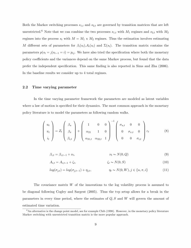
Both the Markov switching processes s1,t and s2,t are governed by transition matrices that are left

unrestricted.6 Note that we can combine the two processes s1,t with M1 regimes and s2,t with M2

regimes into the process st with M = M1 x M2 regimes. Thus the estimation involves estimating

M different sets of parameters for βi(st),Ai(st) and Σ(st). The transition matrix contains the

parameters p(st = j|st−1 = i) = pij . We have also tried the specification where both the monetary

policy coefficients and the variances depend on the same Markov process, but found that the data

prefer the independent specification. This same finding is also reported in Sims and Zha (2006).

In the baseline results we consider up to 4 total regimes.

2.2 Time varying parameter

In the time varying parameter framework the parameters are modeled as latent variables

where a law of motion is specified for their dynamics. The most common approach in the monetary

policy literature is to model the parameters as following random walks.

ut

πt

it

= Zt

βu

βπ

βi,t

+

1 0 0

α21 1 0

α31,t α32,t 1

−1

σu,t 0 0

0 σπ,t 0

0 0 σi,t

εt (8)

βi,t = βi,t−1 + νt, νt ∼ N(0, Q) (9)

Ai,t = Ai,t−1 + ζt, ζt ∼ N(0, S) (10)

log(σj,t) = log(σj,t−1) + ηj,t, ηt ∼ N(0,W ), j ∈ u, π, i (11)

The covariance matrix W of the innovations to the log volatility process is assumed to

be diagonal following Cogley and Sargent (2005). Thus the tvp setup allows for a break in the

parameters in every time period, where the estimates of Q,S and W will govern the amount of

estimated time variation.

6An alternative is the change point model, see for example Chib (1998). However, in the monetary policy literatureMarkov switching with unrestricted transition matrix is the more popular approach.

9

3 Priors and Estimation

3.1 Priors

For the rs case we use symmetric priors, so that regardless of the regime the prior distribution

is the same. For the coefficients we use the so-called “Minnesota” style prior, which provides

shrinkage towards a random walk.7 Specifically the coefficients of the VAR are assumed to follow a

normal prior β ∼ N(mβ,Mβ). Note that the β includes the parameters of both the monetary and

non-monetary equations. mβ is set to 1 for the parameters corresponding to the first own lag and

the rest are set to zero. The prior variance for coefficients of each equation is set in the following

way.√Mβ = λ0λ1

δjL(j)λ3

where δj is the standard deviation of a univariate autoregression of equation

j and L(j) represents the order of the lag in equation j. This prior variance embodies the idea that

own lags are more likely to be important predictors than lags of other variables and the predictive

power diminishes as the lag length increases. Following Sims and Zha (1998) we set λ0 = 1, λ1 = 0.2

and λ2 = λ3 = λ4 = 1. The parameters of the A matrix are assumed to have a normal prior with

mean zero and a large variance. The inverse of the standard deviations σ−1j are assumed to have a

Gamma prior, again with priors being symmetric across regimes. Finally for the transition matrix

P which contains the regime probabilities pi,j we use a Beta prior when there are two regimes and

a Dirichlet prior when there are more than two regimes. The prior parameter vector α of the Beta

and Dirichlet distributions are set so that they imply a probability of 0.85 of staying in the same

regime and an equal probability of 1−0.85M−1 of moving to any another regime, where M is the total

number of regimes. The priors are thus summarized as follows with VA = 10, 000, k = θ = 1 and

mβ, Mβ and α set as described above

A ∼ N(0, VA) (12)

β ∼ N(mβ,Mβ) (13)

σ−1j ∼ G(k, θ) (14)

P ∼ Dir(α) (15)

7As a robustness test, we have also used a training sample prior which gives similar results.

10

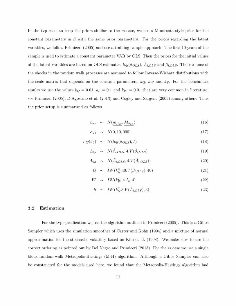
In the tvp case, to keep the priors similar to the rs case, we use a Minnesota-style prior for the

constant parameters in β with the same prior parameters. For the priors regarding the latent

variables, we follow Primiceri (2005) and use a training sample approach. The first 10 years of the

sample is used to estimate a constant parameter VAR by OLS. Then the priors for the initial values

of the latent variables are based on OLS estimates, log(σOLS), Ai,OLS and βi,OLS . The variance of

the shocks in the random walk processes are assumed to follow Inverse-Wishart distributions with

the scale matrix that depends on the constant parameters, kQ, kW and kS . For the benchmark

results we use the values kQ = 0.01, kS = 0.1 and kW = 0.01 that are very common in literature,

see Primiceri (2005), D’Agostino et al. (2013) and Cogley and Sargent (2005) among others. Thus

the prior setup is summarized as follows

βuπ ∼ N(mβuπ ,Mβuπ) (16)

α21 ∼ N(0, 10, 000) (17)

log(σ0) ∼ N(log(σOLS), I) (18)

β0,i ∼ N(βi,OLS , 4.V (βi,OLS) (19)

A0,i ∼ N(Ai,OLS , 4.V (Ai,OLS)) (20)

Q ∼ IW (k2Q.40.V (βi,OLS), 40) (21)

W ∼ IW (k2W .4.In, 4) (22)

S ∼ IW (k2S .3.V (Ai,OLS), 3) (23)

3.2 Estimation

For the tvp specification we use the algorithm outlined in Primiceri (2005). This is a Gibbs

Sampler which uses the simulation smoother of Carter and Kohn (1994) and a mixture of normal

approximation for the stochastic volatility based on Kim et al. (1998). We make sure to use the

correct ordering as pointed out by Del Negro and Primiceri (2013). For the rs case we use a single

block random-walk Metropolis-Hastings (M-H) algorithm. Although a Gibbs Sampler can also

be constructed for the models used here, we found that the Metropolis-Hastings algorithm had

11

good convergence properties and was much more convenient to use.8 All the estimation details are

provided in an online appendix.

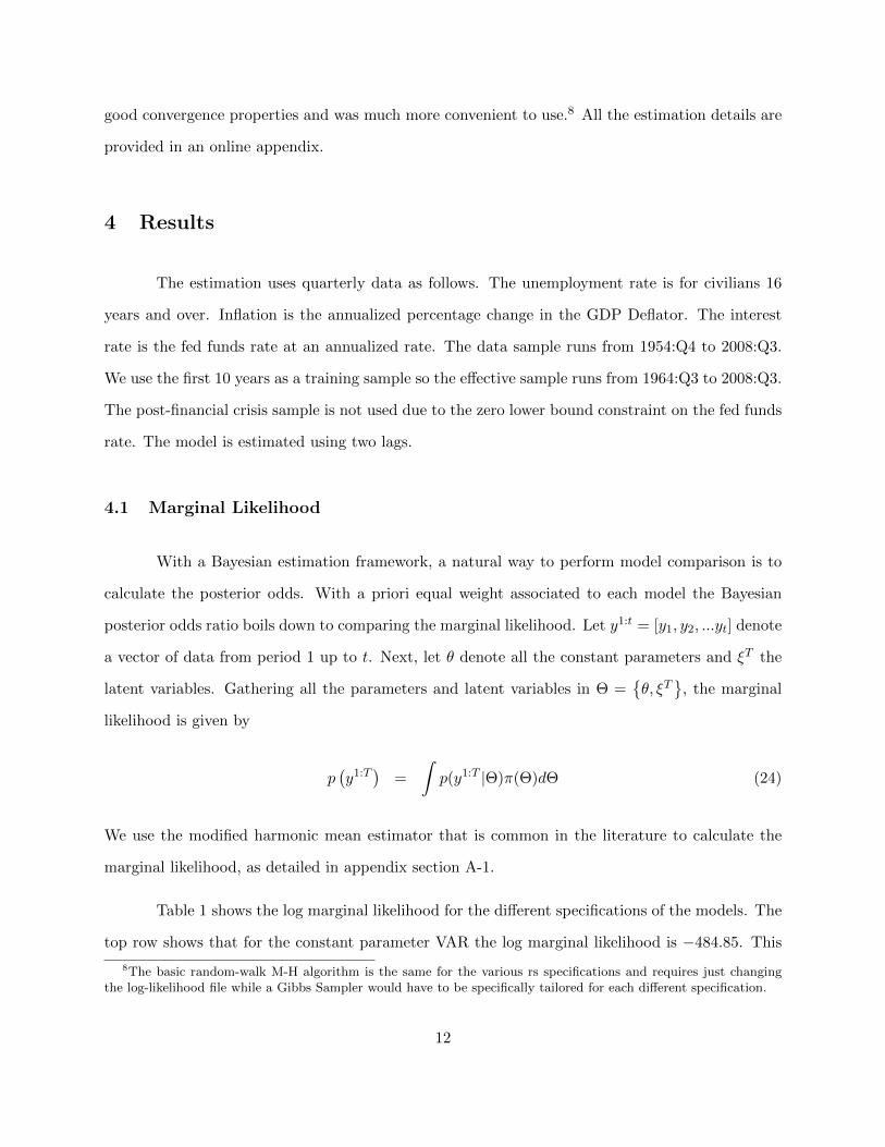
4 Results

The estimation uses quarterly data as follows. The unemployment rate is for civilians 16

years and over. Inflation is the annualized percentage change in the GDP Deflator. The interest

rate is the fed funds rate at an annualized rate. The data sample runs from 1954:Q4 to 2008:Q3.

We use the first 10 years as a training sample so the effective sample runs from 1964:Q3 to 2008:Q3.

The post-financial crisis sample is not used due to the zero lower bound constraint on the fed funds

rate. The model is estimated using two lags.

4.1 Marginal Likelihood

With a Bayesian estimation framework, a natural way to perform model comparison is to

calculate the posterior odds. With a priori equal weight associated to each model the Bayesian

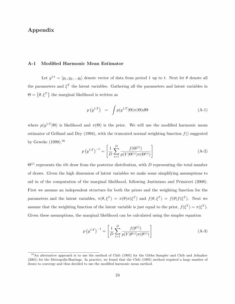
posterior odds ratio boils down to comparing the marginal likelihood. Let y1:t = [y1, y2, ...yt] denote

a vector of data from period 1 up to t. Next, let θ denote all the constant parameters and ξT the

latent variables. Gathering all the parameters and latent variables in Θ =θ, ξT

, the marginal

likelihood is given by

p(y1:T

)=

∫p(y1:T |Θ)π(Θ)dΘ (24)

We use the modified harmonic mean estimator that is common in the literature to calculate the

marginal likelihood, as detailed in appendix section A-1.

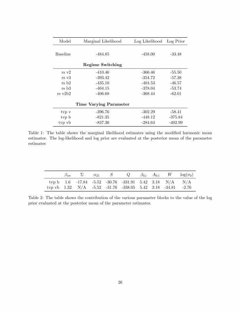
Table 1 shows the log marginal likelihood for the different specifications of the models. The

top row shows that for the constant parameter VAR the log marginal likelihood is −484.85. This

8The basic random-walk M-H algorithm is the same for the various rs specifications and requires just changingthe log-likelihood file while a Gibbs Sampler would have to be specifically tailored for each different specification.

12

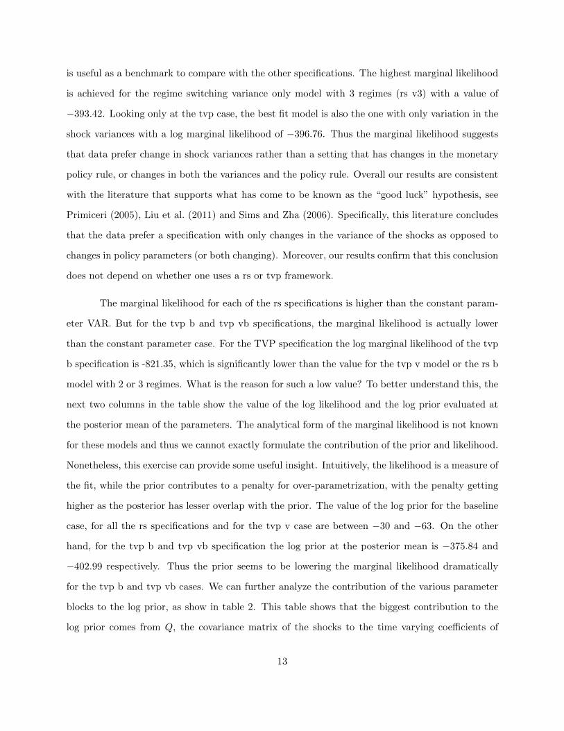
is useful as a benchmark to compare with the other specifications. The highest marginal likelihood

is achieved for the regime switching variance only model with 3 regimes (rs v3) with a value of

−393.42. Looking only at the tvp case, the best fit model is also the one with only variation in the

shock variances with a log marginal likelihood of −396.76. Thus the marginal likelihood suggests

that data prefer change in shock variances rather than a setting that has changes in the monetary

policy rule, or changes in both the variances and the policy rule. Overall our results are consistent

with the literature that supports what has come to be known as the “good luck” hypothesis, see

Primiceri (2005), Liu et al. (2011) and Sims and Zha (2006). Specifically, this literature concludes

that the data prefer a specification with only changes in the variance of the shocks as opposed to

changes in policy parameters (or both changing). Moreover, our results confirm that this conclusion

does not depend on whether one uses a rs or tvp framework.

The marginal likelihood for each of the rs specifications is higher than the constant param-

eter VAR. But for the tvp b and tvp vb specifications, the marginal likelihood is actually lower

than the constant parameter case. For the TVP specification the log marginal likelihood of the tvp

b specification is -821.35, which is significantly lower than the value for the tvp v model or the rs b

model with 2 or 3 regimes. What is the reason for such a low value? To better understand this, the

next two columns in the table show the value of the log likelihood and the log prior evaluated at

the posterior mean of the parameters. The analytical form of the marginal likelihood is not known

for these models and thus we cannot exactly formulate the contribution of the prior and likelihood.

Nonetheless, this exercise can provide some useful insight. Intuitively, the likelihood is a measure of

the fit, while the prior contributes to a penalty for over-parametrization, with the penalty getting

higher as the posterior has lesser overlap with the prior. The value of the log prior for the baseline

case, for all the rs specifications and for the tvp v case are between −30 and −63. On the other

hand, for the tvp b and tvp vb specification the log prior at the posterior mean is −375.84 and

−402.99 respectively. Thus the prior seems to be lowering the marginal likelihood dramatically

for the tvp b and tvp vb cases. We can further analyze the contribution of the various parameter

blocks to the log prior, as show in table 2. This table shows that the biggest contribution to the

log prior comes from Q, the covariance matrix of the shocks to the time varying coefficients of

13

the monetary policy rule. One concern is that large negative values reflect a situation where the

posterior distribution of Q has very little overlap with the prior distribution. To investigate this,

we consider the following exercise. Q has an Inverse-Wishart prior, Q ∼ IW (ν,Q) with shape pa-

rameter ν = 40 and scale matrix Q = k2Q.40.V (βi,OLS) which depends on the variance of coefficients

from a training sample regression, as explained in section 3.1. We can evaluate the log density of

this prior distribution at the mode which is given by Q(ν − 7− 1). The log prior density evaluated

at the mode is -327.99, which is not much higher than the values −375.84 and −402.99 reported in

table 1. In other words, the posterior distribution of Q has reasonable overlap with the specified

prior distribution. Taking this idea a step further we can consider a hypothetical situation where

the prior distribution is the same as the estimated posterior. Even in this case the log prior density

at the mode is not high enough to change our conclusion. This suggests that by construction the

Inverse-Wishart prior adds a relatively large penalty compared to the other parameter blocks. Since

the Inverse-Wishart distribution is very common in the time varying parameter literature, this is

an important consideration for any studies that use the marginal likelihood for model comparison.

There are papers that have hinted at the sensitivity of the marginal likelihood to priors for tvp

models without showing the contribution of the priors, see Campolieti et al. (2014) and Koop et al.

(2009) among others.9 One option is to use simple alternative measures like the Bayesian Informa-

tion Criterion or the expected Log Likelihood. Another option is to use the predictive density, as

we discuss in the next subsection.

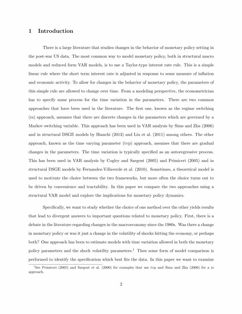
To shed a little more light on the fit of the different models, figure 1 plots the conditional

log density of the tth observation, evaluated at the posterior mean of the estimates. The axes in

each row of the figure are set to the same values for ease of comparison. A common theme is that

the conditional log density value is low for all specifications around 1980 with the lowest value

reached in 1980:Q4. This coincides with the reserves targeting experiment in the early years of

Paul Volcker’s regime. For the tvp models there is also a dip in the conditional log density around

1975 (especially for the tvp v model) while the regime switching models tend to fit well during this

9Additionally, Chan and Grant (2015) show in a simulation study that the marginal likelihood estimates can havea significant bias but their study uses a simpler unobserved components model.

14

period. As will be clear from figures and discussion below, this is because the regime switching

models are good at capturing big abrupt changes while the tvp model is designed to better capture

gradual movements.

4.2 Forecast Performance and Predictive Likelihood

In this section we take advantage of the Bayesian estimation framework and analyze the

posterior predictive density. There are two main reasons for this. First, this helps in comparing

the forecasting performance of the different models. Second, we can get an alternative estimate

of the marginal likelihood by exploiting a decomposition that relates the marginal likelihood to

the one step ahead predictive likelihoods. These exercises require the use of a recursive estimation

scheme as performed in Clark and Ravazzolo (2014) and D’Agostino et al. (2013). For the first run

we estimate the model using data from 1965:Q3 to 1975:Q3. Then we add 1 quarter of data and

re-estimate the model using data from 1965:Q3 to 1975:Q4, and so on till the last run where the

full sample is used.

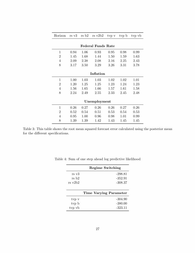
First, using these estimates we forecast up to 8 quarters ahead. The forecast performance

is evaluated using the root mean square forecast error (rmsfe). The numbers are reported in

table 3. We will focus on the results for the fed funds rate but results for unemployment and

inflation are provided as well. First comparing across the rs and tvp specifications, we notice

that the rmsfe (for all horizons) are lower for rs models with changing variances compared to the

corresponding tvp specifications. This suggests that in addition to providing a better in sample fit,

the rs models with changing variances also perform well out of sample. Within the rs specifications,

the rs v3 model provides the best forecasts and allowing for time variation in the monetary policy

parameters increases the rmsfe. This is consistent with the picture emerging from the marginal

likelihood calculations. Now turning to comparison within tvp models, we notice that the forecast

performance aligns with the marginal likelihood comparison as well. But here the values of the

rmsfe for the three different specifications are closer to each other. One way to highlight this is to

notice that the rmsfe for the tvp b model is actually lower than that for the rs b2 model, whereas the

15

marginal likelihood suggested a better fit for the rs b2 model. Overall, the forecasting exercise gives

results that are consistent with the marginal likelihood calculations using the modified harmonic

mean estimator.

Next we consider the predictive likelihood. Appendix section A-2 shows the details of how

the predictive likelihood is evaluated. The evaluation of the one step ahead predictive likelihood

(PL(t)) provides an alternative way to calculate the marginal likelihood. It can be shown that (for

example see Geweke and Amisano (2010))

log p(yt1:T ) =

T∑t=t1

logPL(t) (25)

Thus the log marginal likelihood for estimation using data from t1 (1975:Q3) to T (2008:Q3) is the

sum of the one step ahead log predictive likelihoods from the recursive forecasting exercise. Note

that this number is not directly comparable to the marginal likelihood numbers reported in table

1, where the full sample 1965:Q3 to 2008:Q3 is used. Nevertheless, given the high overlap with the

full sample, the sum above should provide a good indicator of the fit of the model. This sum of the

log predictive likelihoods is reported in table 4. Comparing within the rs and tvp framework, we

conclude that the variance only models have the best fit, consistent with the marginal likelihood

conclusions obtained from table 1. Moreover, the ranking of the three different specifications for

the rs models is the same as that implied by table 1(rs v fits best, followed by rs vb and then rs

b2). However for the tvp models, the order of tvp b and tvp vb is switched. Interestingly, we do

not observe the big deterioration of the marginal likelihood for the tvp b and tvp vb cases that was

observed with the modified harmonic mean estimator. This suggests that the “penalty” imposed by

the Inverse-Wishart prior specification on the marginal likelihood seems to be particularly affecting

the modified harmonic mean estimator and does not negatively affect the predictive density of the

model as much.

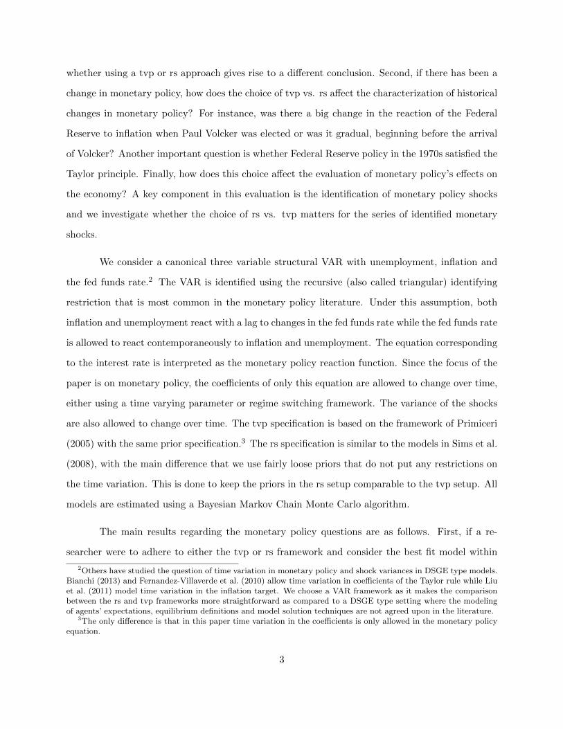
An added advantage of the predictive likelihood decomposition is that it can shed light on

how individual data observations contribute to the evidence for each model. Figure 2 shows the

one-step ahead log predictive likelihood for each time period. The y-axes are aligned to the same

16

values for each row in the figure. As was seen in figure 1, it is clear that predictive likelihood is

the lowest around the end of 1980. What is striking is the magnitude of the contribution of one

single data point in lowering the evidence for the tvp model: 1980:Q4. In other words, once you

ignore the 1980:Q4 observation, then the predictive likelihood evidence for the rs and tvp models is

very close indeed. As will be discussed in the next subsection, the rs models display quick switches

between regimes around the end of 1980 (see figures 3 and 6). On the other hand, the tvp models

cannot account for large discrete changes (see figures 4 and 6 ). This fact explains the superior

performance of the rs models around the end of 1980.

In terms of forecasting performance for the tvp models, our results are consistent with Clark

and Ravazzolo (2014), who find that the VAR with stochastic volatility in the shocks outperforms

a VAR where both the parameters and variance of shocks are allowed to change. Additionally,

Giordani and Villani (2010) find that models that allow large infrequent shifts in the variance of

the shocks outperform gradual continuous movements. This is also consistent with our results from

tables 1,3 and 4 and figure 2. Similar to our paper, these two studies use US data. On the other

hand, for UK data, Barnett et al. (2014) find that the tvp models outperform rs models in terms

of forecasting. Although their specification of regime switching uses the change point framework.

This specification puts restrictions on the transition matrix of the regime indicator, which rules out

transitions to past regimes.

Based on the results in this section, we can make some simple recommendations for applied

researchers who care about the fit of the model and forecasting performance. Models with changes

in shock variance are the best fit models for both rs and tvp specifications. Moreover, if the

researcher does not have any a priori reason for choosing rs or tvp models, then we recommend

using the rs specification. For researchers that insist on using a specification with changes in

the monetary policy rule, the results still suggest using a rs approach from a fit and forecasting

perspective.10 Next, we analyze whether the choice of tvp vs. rs has important implications for

structural questions of interest. The typical strategy in the empirical literature is to consider

either the rs or the tvp framework and conduct analysis of economic issues within that particular

10See subsection 4.4 for monetary policy implications of choosing rs vs tvp within this class of models.

17

framework. Armed with the same underlying VAR model, identifying assumptions, data sample

and priors (as much as possible) we can now evaluate whether researchers conducting analysis in

only the rs framework or tvp framework would arrive at the same answers to important questions

of interest.

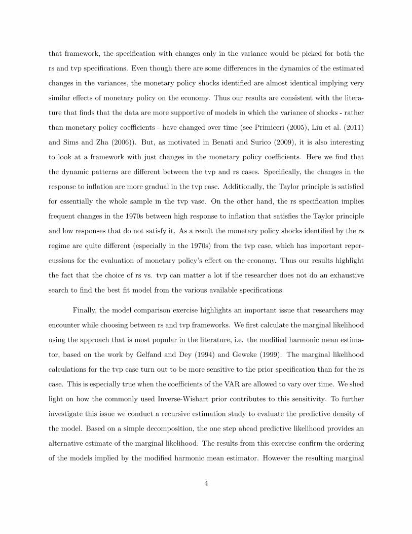
4.3 Change in Shock Variances

The best fit model in both the rs and tvp framework is the variance only model and we

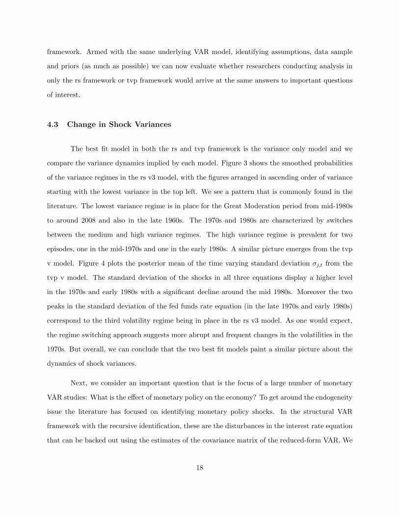
compare the variance dynamics implied by each model. Figure 3 shows the smoothed probabilities

of the variance regimes in the rs v3 model, with the figures arranged in ascending order of variance

starting with the lowest variance in the top left. We see a pattern that is commonly found in the

literature. The lowest variance regime is in place for the Great Moderation period from mid-1980s

to around 2008 and also in the late 1960s. The 1970s and 1980s are characterized by switches

between the medium and high variance regimes. The high variance regime is prevalent for two

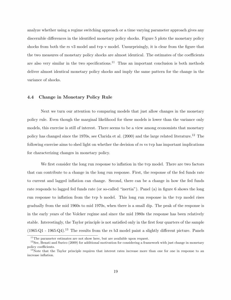
episodes, one in the mid-1970s and one in the early 1980s. A similar picture emerges from the tvp

v model. Figure 4 plots the posterior mean of the time varying standard deviation σj,t from the

tvp v model. The standard deviation of the shocks in all three equations display a higher level

in the 1970s and early 1980s with a significant decline around the mid 1980s. Moreover the two

peaks in the standard deviation of the fed funds rate equation (in the late 1970s and early 1980s)

correspond to the third volatility regime being in place in the rs v3 model. As one would expect,

the regime switching approach suggests more abrupt and frequent changes in the volatilities in the

1970s. But overall, we can conclude that the two best fit models paint a similar picture about the

dynamics of shock variances.

Next, we consider an important question that is the focus of a large number of monetary

VAR studies: What is the effect of monetary policy on the economy? To get around the endogeneity

issue the literature has focused on identifying monetary policy shocks. In the structural VAR

framework with the recursive identification, these are the disturbances in the interest rate equation

that can be backed out using the estimates of the covariance matrix of the reduced-form VAR. We

18

analyze whether using a regime switching approach or a time varying parameter approach gives any

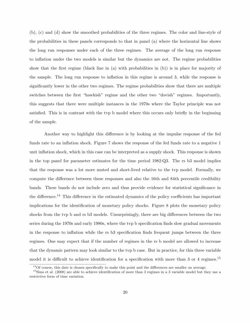
discernible differences in the identified monetary policy shocks. Figure 5 plots the monetary policy

shocks from both the rs v3 model and tvp v model. Unsurprisingly, it is clear from the figure that

the two measures of monetary policy shocks are almost identical. The estimates of the coefficients

are also very similar in the two specifications.11 Thus an important conclusion is both methods

deliver almost identical monetary policy shocks and imply the same pattern for the change in the

variance of shocks.

4.4 Change in Monetary Policy Rule

Next we turn our attention to comparing models that just allow changes in the monetary

policy rule. Even though the marginal likelihood for these models is lower than the variance only

models, this exercise is still of interest. There seems to be a view among economists that monetary

policy has changed since the 1970s, see Clarida et al. (2000) and the large related literature.12 The

following exercise aims to shed light on whether the decision of rs vs tvp has important implications

for characterizing changes in monetary policy.

We first consider the long run response to inflation in the tvp model. There are two factors

that can contribute to a change in the long run response. First, the response of the fed funds rate

to current and lagged inflation can change. Second, there can be a change in how the fed funds

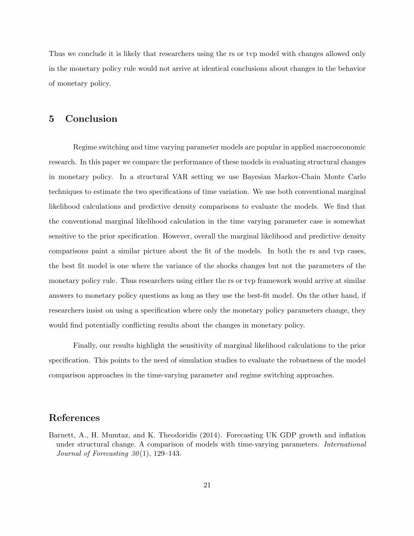
rate responds to lagged fed funds rate (or so-called “inertia”). Panel (a) in figure 6 shows the long

run response to inflation from the tvp b model. This long run response in the tvp model rises

gradually from the mid 1960s to mid 1970s, when there is a small dip. The peak of the response is

in the early years of the Volcker regime and since the mid 1980s the response has been relatively

stable. Interestingly, the Taylor principle is not satisfied only in the first four quarters of the sample

(1965:Q1 - 1965:Q4).13 The results from the rs b3 model paint a slightly different picture. Panels

11The parameter estimates are not show here, but are available upon request.12See, Benati and Surico (2009) for additional motivation for considering a framework with just change in monetary

policy coefficients.13Note that the Taylor principle requires that interest rates increase more than one for one in response to an

increase inflation.

19

(b), (c) and (d) show the smoothed probabilities of the three regimes. The color and line-style of

the probabilities in these panels corresponds to that in panel (a) where the horizontal line shows

the long run responses under each of the three regimes. The average of the long run response

to inflation under the two models is similar but the dynamics are not. The regime probabilities

show that the first regime (black line in (a) with probabilities in (b)) is in place for majority of

the sample. The long run response to inflation in this regime is around 3, while the response is

significantly lower in the other two regimes. The regime probabilities show that there are multiple

switches between the first “hawkish” regime and the other two “dovish” regimes. Importantly,

this suggests that there were multiple instances in the 1970s where the Taylor principle was not

satisfied. This is in contrast with the tvp b model where this occurs only briefly in the beginning

of the sample.

Another way to highlight this difference is by looking at the impulse response of the fed

funds rate to an inflation shock. Figure 7 shows the response of the fed funds rate to a negative 1

unit inflation shock, which in this case can be interpreted as a supply shock. This response is shown

in the top panel for parameter estimates for the time period 1982:Q3. The rs b3 model implies

that the response was a lot more muted and short-lived relative to the tvp model. Formally, we

compute the difference between these responses and also the 16th and 84th percentile credibility

bands. These bands do not include zero and thus provide evidence for statistical significance in

the difference.14 This difference in the estimated dynamics of the policy coefficients has important

implications for the identification of monetary policy shocks. Figure 8 plots the monetary policy

shocks from the tvp b and rs b3 models. Unsurprisingly, there are big differences between the two

series during the 1970s and early 1980s, where the tvp b specification finds slow gradual movements

in the response to inflation while the rs b3 specification finds frequent jumps between the three

regimes. One may expect that if the number of regimes in the rs b model are allowed to increase

that the dynamic pattern may look similar to the tvp b case. But in practice, for this three variable

model it is difficult to achieve identification for a specification with more than 3 or 4 regimes.15

14Of course, this date is chosen specifically to make this point and the differences are smaller on average.15Sims et al. (2008) are able to achieve identification of more than 3 regimes in a 3 variable model but they use a

restrictive form of time variation.

20

Thus we conclude it is likely that researchers using the rs or tvp model with changes allowed only

in the monetary policy rule would not arrive at identical conclusions about changes in the behavior

of monetary policy.

5 Conclusion

Regime switching and time varying parameter models are popular in applied macroeconomic

research. In this paper we compare the performance of these models in evaluating structural changes

in monetary policy. In a structural VAR setting we use Bayesian Markov-Chain Monte Carlo

techniques to estimate the two specifications of time variation. We use both conventional marginal

likelihood calculations and predictive density comparisons to evaluate the models. We find that

the conventional marginal likelihood calculation in the time varying parameter case is somewhat

sensitive to the prior specification. However, overall the marginal likelihood and predictive density

comparisons paint a similar picture about the fit of the models. In both the rs and tvp cases,

the best fit model is one where the variance of the shocks changes but not the parameters of the

monetary policy rule. Thus researchers using either the rs or tvp framework would arrive at similar

answers to monetary policy questions as long as they use the best-fit model. On the other hand, if

researchers insist on using a specification where only the monetary policy parameters change, they

would find potentially conflicting results about the changes in monetary policy.

Finally, our results highlight the sensitivity of marginal likelihood calculations to the prior

specification. This points to the need of simulation studies to evaluate the robustness of the model

comparison approaches in the time-varying parameter and regime switching approaches.

References

Barnett, A., H. Mumtaz, and K. Theodoridis (2014). Forecasting UK GDP growth and inflationunder structural change. A comparison of models with time-varying parameters. InternationalJournal of Forecasting 30 (1), 129–143.

21

Benati, L. and P. Surico (September 2009). VAR Analysis and the Great Moderation. The AmericanEconomic Review 99, 1636–1652(17).

Bianchi, F. (2013). Regime Switches, Agents’ Beliefs, and Post-World War II U.S. MacroeconomicDynamics. The Review of Economic Studies 80 (2), 463–490.

Campolieti, M., D. Gefang, and G. Koop (2014). Time variation in the dynamics of worker flows:evidence from North America and Europe. Journal of Applied Econometrics 29 (2), 265–290.

Carter, C. K. and R. Kohn (1994). On Gibbs sampling for state space models. Biometrika 81 (3),541–553.

Chan, J. C. and A. L. Grant (2015). Pitfalls of estimating the marginal likelihood using the modifiedharmonic mean. Economics Letters 131, 29–33.

Chib, S. (1995). Marginal likelihood from the Gibbs output. Journal of the American StatisticalAssociation 90 (432), 1313–1321.

Chib, S. (1998). Estimation and comparison of multiple change-point models. Journal of Econo-metrics 86 (2), 221–241.

Chib, S. and I. Jeliazkov (2001). Marginal likelihood from the Metropolis–Hastings output. Journalof the American Statistical Association 96 (453), 270–281.

Christiano, L. J., M. Eichenbaum, and C. L. Evans (1999). Monetary policy shocks: What havewe learned and to what end? Handbook of Macroeconomics 1, 65–148.

Clarida, R., J. Gali, and M. Gertler (2000). Monetary policy rules and macroeconomic stability:Evidence and some theory*. Quarterly Journal of Economics 115 (1), 147–180.

Clark, T. E. and F. Ravazzolo (2014). Macroeconomic forecasting performanc under alternativespecifications of time-varying volatility. Journal of Applied Econometrics.

Cogley, T., S. Morozov, and T. J. Sargent (2005). Bayesian fan charts for UK inflation: Forecastingand sources of uncertainty in an evolving monetary system. Journal of Economic Dynamics andControl 29 (11), 1893–1925.

Cogley, T. and T. J. Sargent (2005). Drifts and volatilities: monetary policies and outcomes in thepost WWII US. Review of Economic Dynamics 8 (2), 262 – 302. Monetary Policy and Learning.

D’Agostino, A., L. Gambetti, and D. Giannone (2013). Macroeconomic forecasting and structuralchange. Journal of Applied Econometrics 28 (1), 82–101.

Del Negro, M. and G. Primiceri (2013). Time-varying structural vector autoregressions and mone-tary policy: a corrigendum. Technical report, Staff Report, Federal Reserve Bank of New York.

Fernandez-Villaverde, J., P. Guerron-Quintana, and J. F. Rubio-Ramirez (2010). Fortune or Virtue:Time-Variant Volatilities Versus Parameter Drifting in U.S. Data. SSRN eLibrary .

Gambetti, L., E. Pappa, and F. Canova (2008). The Structural Dynamics of U.S. Output andInflation: What Explains the Changes? Journal of Money, Credit and Banking 40 (2-3), 369–388.

22

Gelfand, A. E. and D. K. Dey (1994). Bayesian model choice: Asymptotics and exact calculations.Journal of the Royal Statistical Society. Series B (Methodological) 56 (3), pp. 501–514.

Geweke, J. (1999). Using simulation methods for bayesian econometric models: inference, develop-ment,and communication. Econometric Reviews 18 (1), 1–73.

Geweke, J. and G. Amisano (2010). Comparing and evaluating Bayesian predictive distributionsof asset returns. International Journal of Forecasting 26 (2), 216–230.

Giordani, P. and M. Villani (2010). Forecasting macroeconomic time series with locally adaptivesignal extraction. International Journal of Forecasting 26 (2), 312–325.

Hamilton, J. D. (2001). A parametric approach to flexible nonlinear inference. Econometrica 69 (3),537–573.

Justiniano, A. and G. E. Primiceri (2008). The time-varying volatility of macroeconomic fluctua-tions. American Economic Review 98 (3), 604–41.

Kim, S., N. Shephard, and S. Chib (1998). Stochastic volatility: Likelihood inference and compar-ison with arch models. The Review of Economic Studies 65 (3), 361–393.

Koop, G., R. Leon-Gonzalez, and R. W. Strachan (2009). On the evolution of the monetary policytransmission mechanism. Journal of Economic Dynamics and Control 33 (4), 997–1017.

Koop, G. and S. Potter (2010). A flexible approach to parametric inference in nonlinear and timevarying time series models. Journal of Econometrics 159 (1), 134–150.

Koop, G. and S. M. Potter (2007). Estimation and forecasting in models with multiple breaks. TheReview of Economic Studies 74 (3), 763–789.

Lhuissier, S. and M. Zabelina (2015). On the stability of Calvo-style Price-Setting Behavior. Journalof Economic Dynamics and Control .

Liu, Z., D. F. Waggoner, and T. Zha (2011). Sources of macroeconomic fluctuations: A regime-switching DSGE approach. Quantitative Economics 2 (2), 251–301.

Primiceri, G. E. (2005). Time varying structural vector autoregressions and monetary policy. Reviewof Economic Studies 72 (3), 821–852.

Sargent, T., N. Williams, and T. Zha (2006). Shocks and government beliefs: The rise and fall ofAmerican inflation. American Economic Review 96 (4), 1193–1224.

Sims, C. A., D. F. Waggoner, and T. Zha (2008). Methods for inference in large multiple-equationmarkov-switching models. Journal of Econometrics 146 (2), 255–274.

Sims, C. A. and T. Zha (1998). Bayesian methods for dynamic multivariate models. InternationalEconomic Review , 949–968.

Sims, C. A. and T. Zha (2006). Were there regime switches in U.S. monetary policy? The AmericanEconomic Review 96 (1), 54–81.

23

Appendix

A-1 Modified Harmonic Mean Estimator

Let y1:t = [y1, y2, ...yt] denote vector of data from period 1 up to t. Next let θ denote all

the parameters and ξT the latent variables. Gathering all the parameters and latent variables in

Θ =θ, ξT

the marginal likelihood is written as

p(y1:T

)=

∫p(y1:T |Θ)π(Θ)dΘ (A-1)

where p(y1:T |Θ) is likelihood and π(Θ) is the prior. We will use the modified harmonic mean

estimator of Gelfand and Dey (1994), with the truncated normal weighting function f() suggested

by Geweke (1999).16

p(y1:T

)−1=

[1

D

D∑i=1

f(Θ(i))

p(Y |Θ(i))π(Θ(i))

](A-2)

Θ(i) represents the ith draw from the posterior distribution, with D representing the total number

of draws. Given the high dimension of latent variables we make some simplifying assumptions to

aid in of the computation of the marginal likelihood, following Justiniano and Primiceri (2008).

First we assume an independent structure for both the priors and the weighting function for the

parameters and the latent variables, π(θ, ξT ) = π(θ)π(ξT ) and f(θ, ξT ) = f(θ)f(ξT ). Next we

assume that the weighting function of the latent variable is just equal to the prior, f(ξT ) = π(ξT ).

Given these assumptions, the marginal likelihood can be calculated using the simpler equation

p(y1:T

)−1=

[1

D

D∑i=1

f(θ(i))

p(Y |θ(i))π(θ(i))

](A-3)

16An alternative approach is to use the method of Chib (1995) for the Gibbs Sampler and Chib and Jeliazkov(2001) for the Metropolis-Hastings. In practice, we found that the Chib (1995) method required a large number ofdraws to converge and thus decided to use the modified harmonic mean method.

24

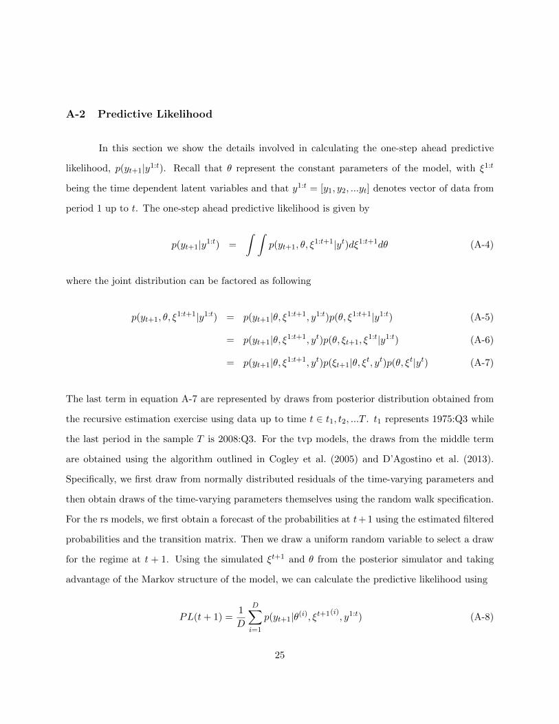
A-2 Predictive Likelihood

In this section we show the details involved in calculating the one-step ahead predictive

likelihood, p(yt+1|y1:t). Recall that θ represent the constant parameters of the model, with ξ1:t

being the time dependent latent variables and that y1:t = [y1, y2, ...yt] denotes vector of data from

period 1 up to t. The one-step ahead predictive likelihood is given by

p(yt+1|y1:t) =

∫ ∫p(yt+1, θ, ξ

1:t+1|yt)dξ1:t+1dθ (A-4)

where the joint distribution can be factored as following

p(yt+1, θ, ξ1:t+1|y1:t) = p(yt+1|θ, ξ1:t+1, y1:t)p(θ, ξ1:t+1|y1:t) (A-5)

= p(yt+1|θ, ξ1:t+1, yt)p(θ, ξt+1, ξ1:t|y1:t) (A-6)

= p(yt+1|θ, ξ1:t+1, yt)p(ξt+1|θ, ξt, yt)p(θ, ξt|yt) (A-7)

The last term in equation A-7 are represented by draws from posterior distribution obtained from

the recursive estimation exercise using data up to time t ∈ t1, t2, ...T . t1 represents 1975:Q3 while

the last period in the sample T is 2008:Q3. For the tvp models, the draws from the middle term

are obtained using the algorithm outlined in Cogley et al. (2005) and D’Agostino et al. (2013).

Specifically, we first draw from normally distributed residuals of the time-varying parameters and

then obtain draws of the time-varying parameters themselves using the random walk specification.

For the rs models, we first obtain a forecast of the probabilities at t+ 1 using the estimated filtered

probabilities and the transition matrix. Then we draw a uniform random variable to select a draw

for the regime at t + 1. Using the simulated ξt+1 and θ from the posterior simulator and taking

advantage of the Markov structure of the model, we can calculate the predictive likelihood using

PL(t+ 1) =1

D

D∑i=1

p(yt+1|θ(i), ξt+1(i), y1:t) (A-8)

25

Model Marginal Likelihood Log Likelihood Log Prior

Baseline -484.85 -458.00 -33.48

Regime Switching

rs v2 -410.46 -366.46 -55.50rs v3 -393.42 -354.72 -57.38rs b2 -435.10 -404.53 -46.57rs b3 -404.15 -378.04 -53.74

rs v2b2 -406.68 -368.44 -62.01

Time Varying Parameter

tvp v -396.76 -302.29 -58.41tvp b -821.35 -448.12 -375.84

tvp vb -837.36 -284.64 -402.99

Table 1: The table shows the marginal likelihood estimates using the modified harmonic meanestimator. The log-likelihood and log prior are evaluated at the posterior mean of the parameterestimates

βuπ Σ α21 S Q β0,i A0,i W log(σ0)

tvp b 1.6 -17.84 -5.52 -30.76 -331.91 5.42 3.18 N/A N/Atvp vb 1.32 N/A -5.52 -31.76 -338.05 5.42 3.18 -34.81 -2.76

Table 2: The table shows the contribution of the various parameter blocks to the value of the logprior evaluated at the posterior mean of the parameter estimates.

26

Horizon rs v3 rs b2 rs v2b2 tvp v tvp b tvp vb

Federal Funds Rate

1 0.94 1.06 0.93 0.95 0.98 0.992 1.45 1.68 1.44 1.50 1.59 1.634 2.09 2.38 2.08 2.16 2.25 2.438 3.17 3.50 3.29 3.26 3.31 3.78

Inflation

1 1.00 1.03 1.03 1.02 1.02 1.012 1.20 1.25 1.25 1.23 1.24 1.234 1.56 1.65 1.66 1.57 1.61 1.588 2.24 2.49 2.55 2.33 2.45 2.48

Unemployment

1 0.26 0.27 0.26 0.26 0.27 0.262 0.52 0.54 0.51 0.53 0.54 0.534 0.95 1.00 0.96 0.98 1.01 0.998 1.39 1.39 1.42 1.43 1.45 1.45

Table 3: This table shows the root mean squared forecast error calculated using the posterior meanfor the different specifications.

Table 4: Sum of one step ahead log predictive likelihood

Regime Switching

rs v3 -298.81rs b2 -352.91

rs v2b2 -308.37

Time Varying Parameter

tvp v -304.90tvp b -380.00

tvp vb -323.11

27

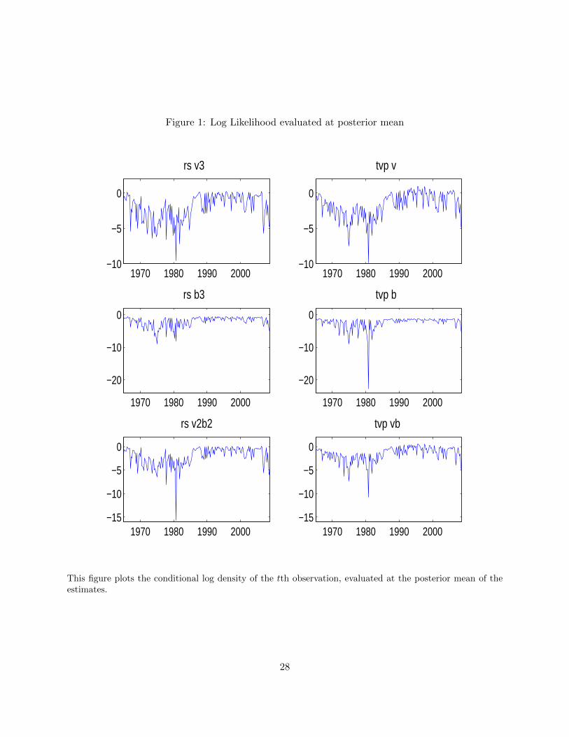
Figure 1: Log Likelihood evaluated at posterior mean

1970 1980 1990 2000−10

−5

0

rs v3

1970 1980 1990 2000−10

−5

0

tvp v

1970 1980 1990 2000

−20

−10

0

rs b3

1970 1980 1990 2000

−20

−10

0

tvp b

1970 1980 1990 2000−15

−10

−5

0

rs v2b2

1970 1980 1990 2000−15

−10

−5

0

tvp vb

This figure plots the conditional log density of the tth observation, evaluated at the posterior mean of theestimates.

28

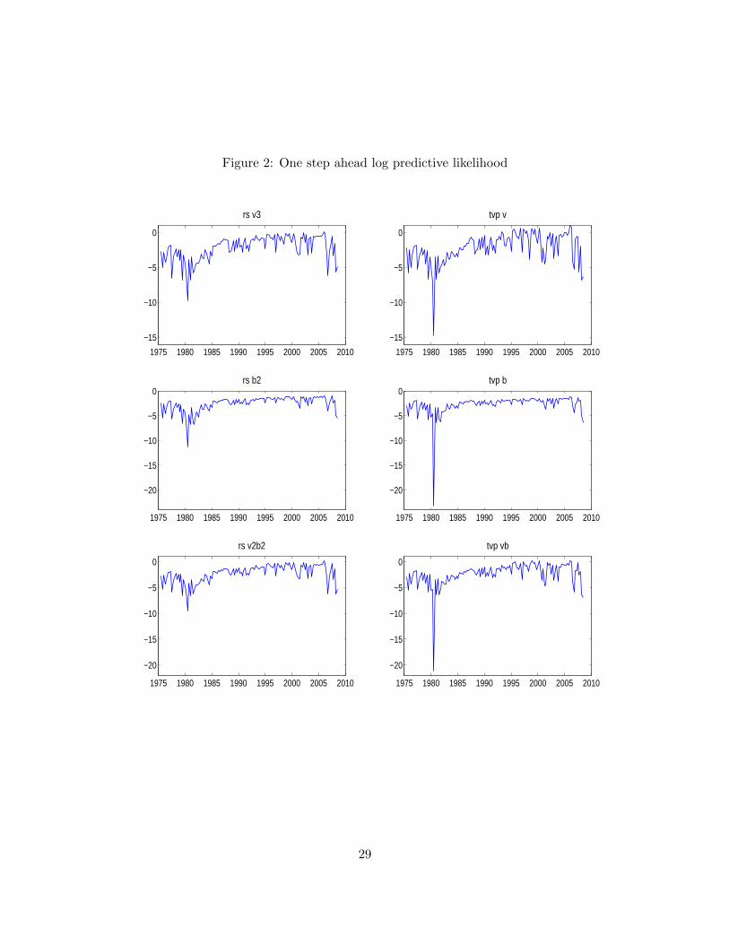
Figure 2: One step ahead log predictive likelihood

1975 1980 1985 1990 1995 2000 2005 2010

−15

−10

−5

0

rs v3

1975 1980 1985 1990 1995 2000 2005 2010

−15

−10

−5

0

tvp v

1975 1980 1985 1990 1995 2000 2005 2010

−20

−15

−10

−5

0rs b2

1975 1980 1985 1990 1995 2000 2005 2010

−20

−15

−10

−5

0tvp b

1975 1980 1985 1990 1995 2000 2005 2010

−20

−15

−10

−5

0

rs v2b2

1975 1980 1985 1990 1995 2000 2005 2010

−20

−15

−10

−5

0

tvp vb

29

Figure 3: Smoothed probability of variance regimes

1970 1980 1990 2000

0.2

0.4

0.6

0.8

Low Volatility

1970 1980 1990 2000

0.2

0.4

0.6

0.8

Medium Volatility

1970 1980 1990 2000

0.2

0.4

0.6

0.8

High Volatility

The figure shows the smoothed probability of the variance regimes at the posterior mean from the rs v3model.

30

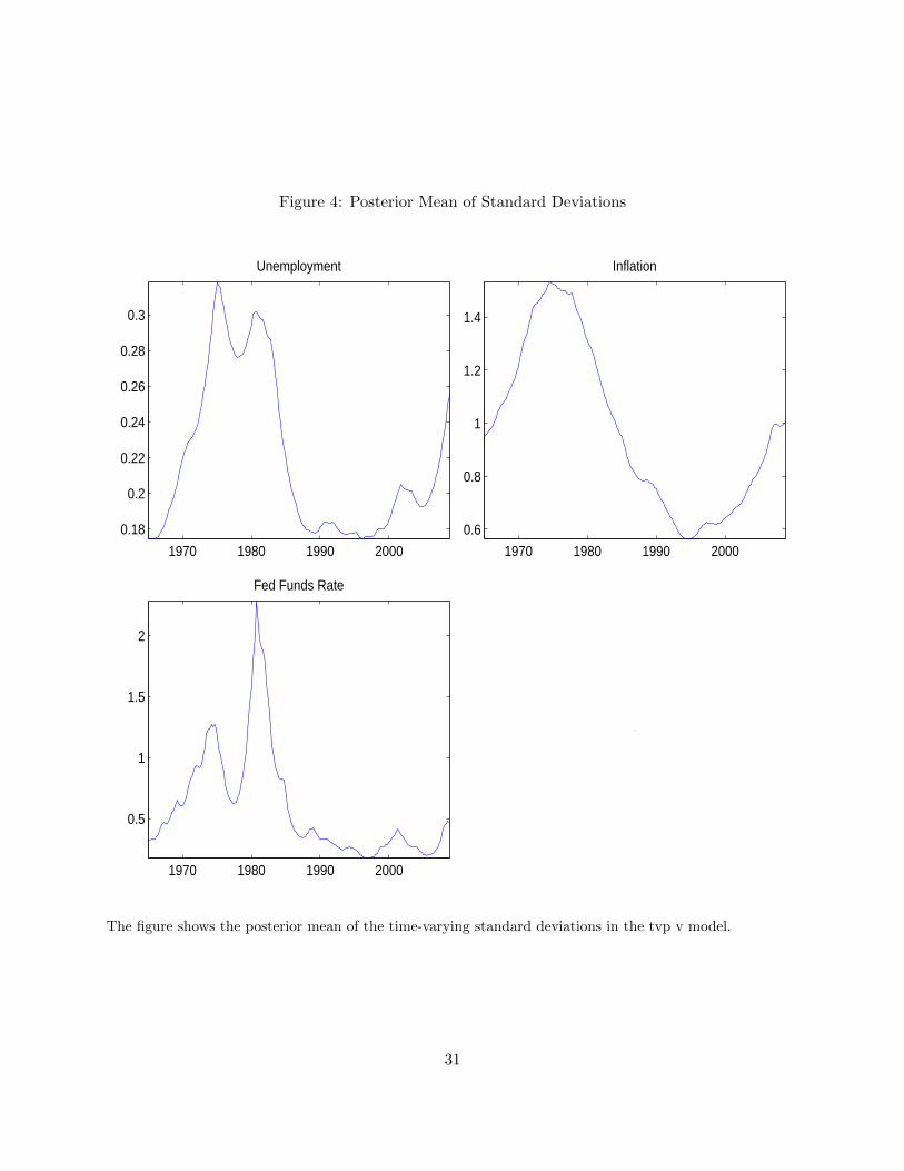
Figure 4: Posterior Mean of Standard Deviations

1970 1980 1990 2000

0.18

0.2

0.22

0.24

0.26

0.28

0.3

Unemployment

1970 1980 1990 2000

0.6

0.8

1

1.2

1.4

Inflation

1970 1980 1990 2000

0.5

1

1.5

2

Fed Funds Rate

The figure shows the posterior mean of the time-varying standard deviations in the tvp v model.

31

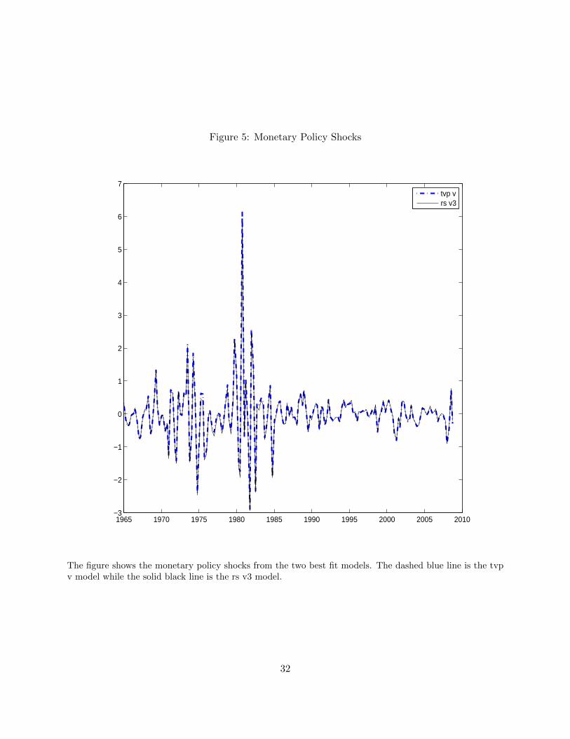
Figure 5: Monetary Policy Shocks

1965 1970 1975 1980 1985 1990 1995 2000 2005 2010−3

−2

−1

0

1

2

3

4

5

6

7

tvp vrs v3

The figure shows the monetary policy shocks from the two best fit models. The dashed blue line is the tvpv model while the solid black line is the rs v3 model.

32

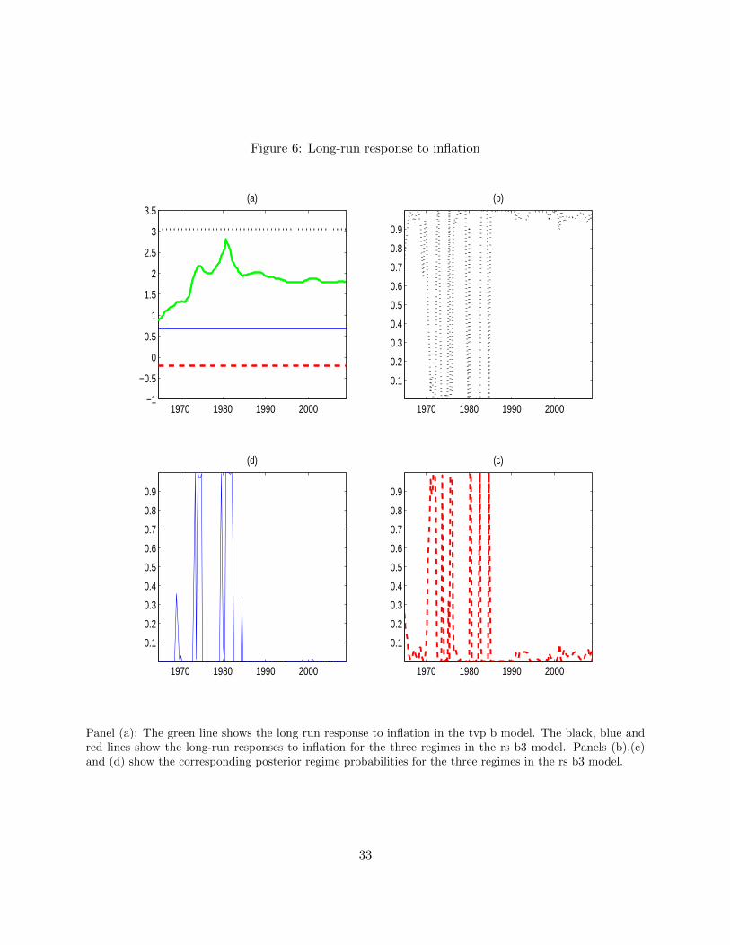
Figure 6: Long-run response to inflation

1970 1980 1990 2000−1

−0.5

0

0.5

1

1.5

2

2.5

3

3.5(a)

1970 1980 1990 2000

0.1

0.2

0.3

0.4

0.5

0.6

0.7

0.8

0.9

(c)

1970 1980 1990 2000

0.1

0.2

0.3

0.4

0.5

0.6

0.7

0.8

0.9

(b)

1970 1980 1990 2000

0.1

0.2

0.3

0.4

0.5

0.6

0.7

0.8

0.9

(d)

Panel (a): The green line shows the long run response to inflation in the tvp b model. The black, blue andred lines show the long-run responses to inflation for the three regimes in the rs b3 model. Panels (b),(c)and (d) show the corresponding posterior regime probabilities for the three regimes in the rs b3 model.

33

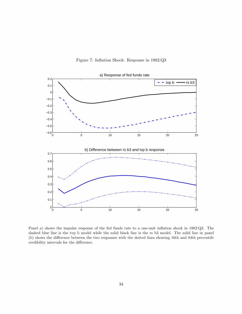
Figure 7: Inflation Shock: Response in 1982:Q3

0 5 10 15 20 25−0.6

−0.5

−0.4

−0.3

−0.2

−0.1

0

0.1

0.2a) Response of fed funds rate

tvp b rs b3

0 5 10 15 20 250

0.1

0.2

0.3

0.4

0.5

0.6

0.7b) Difference between rs b3 and tvp b response

Panel a) shows the impulse response of the fed funds rate to a one-unit inflation shock in 1982:Q3. Thedashed blue line is the tvp b model while the solid black line is the rs b3 model. The solid line in panel(b) shows the difference between the two responses with the dotted lines showing 16th and 84th percentilecredibility intervals for the difference.

34

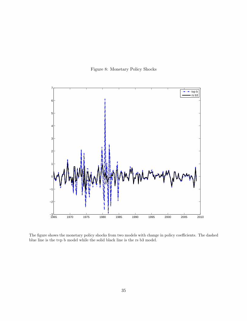
Figure 8: Monetary Policy Shocks

1965 1970 1975 1980 1985 1990 1995 2000 2005 2010−3

−2

−1

0

1

2

3

4

5

6

7

tvp brs b3

The figure shows the monetary policy shocks from two models with change in policy coefficients. The dashedblue line is the tvp b model while the solid black line is the rs b3 model.

35