Modeling Cold Pools in California’s Central Valley

Travis Wilson ∗ and Robert FovellDepartment of Atmospheric and Oceanic Sciences, University of California, Los Angeles

ABSTRACT

Despite our increased understanding in the relevant physical processes, forecasting radiativecold pools and their associated meteorological phenomena (e.g., fog and freezing rain) remains achallenging problem in mesoscale models. The present study is focused on California’s Tule fogwhere the Weather Research and Forecasting (WRF) model’s inability to forecast the event isaddressed and substantially improved. An intra-model physics ensemble reveals that no currentphysics is able to properly capture the Tule fog and that model revisions are necessary. It hasbeen found that revisions to the height of the lowest model level in addition to reconsiderationof horizontal diffusion and surface-atmospheric coupling are critical for accurately forecasting theonset and duration of these events.

1. Introduction

Whiteman et al. (2001) defined a cold pool as a to-pographically confined, stagnant layer of air overlaid bywarmer air aloft. A dramatic and well known example isthe Tule fog of California’s heavily populated Central Val-ley (CV), of which can persist for several days. If a coldpool last longer than one diurnal cycle it is classified asa persistent cold pool, whereas diurnal cold pools form atsunset and decay at sunrise (Whiteman et al. 2001). Whilethe Central Valley is a common example, cold pools aremost prevalent in mountain valleys during periods of highatmospheric pressure, light winds and low solar isolation(Daly et al. 2009). Due to their characteristic inversions,cold pools are also conducive to freezing rain that createsa hazard to transportation and safety (Whiteman et al.2001).

In this paper, an attempt to properly fix the cold poolmodeling problem in California’s CV will be undertaken.Most recently, Ryerson (2012) noted the Weather Researchand Forecasting (WRF) model’s inability to produce fog inand around the CV, which was largely traced to a overnightwarm bias. In order to fix this, he applied post-processingcorrections which added significant overnight skill; how-ever, due to the non-linear evolution of fog, only modestskill increases were seen after sunrise. This paper is not anattempt to amend the cold pool model problem via postprocessing techniques, but rather, by way of model physicsimprovements.

Advancements in modeling cold pools need to be madenot only for forecasting fog and precipitation type, but alsofor air quality as it is of great concern to the U.S. Envi-ronmental Protection Agency (EPA) Office of Air Quality

Planning and Standards (Baker et al. 2011). The meteo-rological conditions associated with cold pools create stag-nant air that cannot mix out vertically due to capping in-versions. This increases ozone or PM2.5 (particulate mat-ter with diameter <2.5 um) concentrations that can exceedthe National Ambient Air Quality Standard (NAAQS) inmany parts of the Western United States including, butnot limited to, the Pacific Northwest, the Central Valley ofCalifornia, and Great Basin (Gillies et al. 2010). Of course,elevated ozone and PM2.5 levels pose a large health risk tomany Americans. Despite the impact they impose on airpollution and weather, persistent cold pools have receivedrelatively little research attention (Zhong et al. 2001).

WRF, along with the Fifth-Generation NCAR/PennState Mesoscale Model (MM5), have failed to reproducethe intensity and persistence of cold pools despite system-atic improvements to both model physical parameteriza-tions as well as horizontal and vertical resolution (Bakeret al. 2011). Data assimilation and surface nudging havealso been explored, both failing to add value to the al-ready poor representation of cold pools (Avery 2011). Ofthe cold pools that are resolved, they often mix out tooearly, leading to erroneous surface temperatures, ozone,and PM2.5 concentrations (Avery 2011). It is becomingincreasingly clear that a cold pool-aware surface and/orboundary layer schemes are needed in WRF to accuratelyreproduce these stagnant air quality episodes (Baker et al.2011; Avery 2011).

The process of cold air pooling can be enhanced by shel-tering from valleys and nearby trees that effectively reducethe vertical mixing that would otherwise bring warmer airdown to the surface (Gustavsson et al. 1998). In addition

1

to this, Whiteman (2000) has demonstrated that furthercooling in valleys is possible simply because of their shape;a cross sectional column of air over a valley is always lessthan that of flat terrain. That said, Whiteman et al. (2004)showed the cooling effect is counteracted by the the down-ward longwave radiation originating not only from the at-mosphere, but also from the valley walls.

The usual conceptual model of cold pool formation invalleys involves cool air drainage. Just after sunset, windsdiminish and a shallow, stable, boundary layer forms dueto the strong radiative flux divergence. Negatively buoyantair originating on the side slopes of the valley descends tothe stable layer, detaches from the side wall, and flows outover the center of the basin (Clements et al. 2003). Essen-tially, the air aloft is efficiently cooled by the basin wallsbefore becoming detached; this acts to enhance the coolingabove the surface due to the sensible heat flux divergence(Whiteman et al. 1996).

Nevertheless, Whiteman et al. (1996) found the sensibleheat flux at the surface to be near zero. Neff and King(1989) produced similar results in their research showingthat drainage flows along the Colorado River basin overlaya stronger surface based inversion of lighter winds. Thissuggests that the cooling above the surface can be due toadvective effects while the cooling at the bottom occursin situ. It should be noted that cooling aloft by drainageflows indirectly assists the in situ cooling at the surface byreducing the downward longwave radiation. Though thiseffect is suspected to be insignificant, it is currently unclearhow important it may be.

Drainage flows do not always become detached fromthe basin walls and have been well observed flowing in val-ley locations (Hootman and Blumen 1983; Gudiksen et al.1992; Bodine et al. 2009). Yet, their role in the productionof cold pools remains controversial. In the 1997 Cooper-ative Atmospheric Surface Exchange Study (CASES-97)at the Walnut River watershed in Kansas, LeMone et al.(2003) attributed cold temperatures at the low elevationsites to cold air drainage and radiative cooling. However,the fast drainage flows observed at higher elevations wereextremely weak lower down, causing the authors to suggestthat the flows were elevated over a more dense cold pool.Mahrt et al. (2001) examined the CASES-99 observationsin south-central Kansas and found that while the drainageflows do exist, their influence on the surface fluxes wereundetectable because the shallow flows decoupled the ob-servations (located at 3-10m) from the surface. It is worthnoting that of the surface fluxes measured, the sensibleheat remained downward-directed; that is, it acted as aheat source throughout the night.

In contrast, earlier research performed by Thompson(1986) suggests that cold pool formation in open and closedvalleys is a direct result of sheltering and not cold airdrainage; the latest research agrees. In the gently slop-

ing terrain of Oklahoma, Hunt et al. (2007) concluded thatthe cooling observed in cold pools occurred in situ whichcounters the results of LeMone et al. (2003). More recently,Bodine et al. (2009) found that cold pools were suppressedby the katabatic winds in the Lake Thunderbird Micronet,a dense collection of surface stations (28 stations) in thegently sloping terrain of Lake Thunderbird, Oklahoma. Infact, they went as far as stating that, “pooling of cold airas a result of drainage flow can clearly be excluded as afactor causing the CP [cold pool] development at the mi-cronet”. Instead, cold pool formation was likely caused bythe cooling that occurred in situ due to the radiative heatloss and diminishing turbulent heat transfer in shelteredregions.

Sometimes, drainage flows are not even observed, asClements et al. (2003) has shown. When inspecting theclosed 1km Peters Sinks basin in Utah, the winds ceasedin the entire basin roughly 2 hours after sunset when theybecame “too weak to measure accurately”. This led totheir conclusion that downslope flows in the Peters Sinksbasin play only a minor role in the formation of cold pools.These weak flows were somewhat expected as Katurji andZhong (2012) have shown that weaker drainage flows docorrespond to smaller basins with larger slope angles intwo-dimensional idealized simulations. Additionally, theyfound the main cooling process near the basin floor (<200m)to be the longwave radiative flux divergence, while the ver-tical advection of temperature dominated the cooling pro-cess in the upper basin area.

Although the production of cold pools may be slightlycontroversial, the latest research agrees that temperaturesare not further reduced due to cold air drainage. This isimportant because if they were, drainage flows of only a fewmeters would be extremely difficult to resolve and wouldsomehow have to be parameterized. However, since thisis not case, we believe cold pools in California’s CentralValley can be resolved with relatively coarse resolution.

2. Methodology

Using WRF version 3.5, cold pools in California’s Cen-tral Valley will be modeled with and without several mod-ifications to the default WRF. Different atmospheric ini-tializations were tested and their influence was deemedrelatively unimportant; because of this, all atmosphericvariables will be initialized from the North American Re-gional Reanalysis (NARR). In contrast, simulations weresensitive to the soil initialization, so we have consequentlychosen to extract these surface fields from a variety ofsources including the NARR, North American Mesoscalemodel (NAM), ERA-Interim, and from offline simulationsspun using NCAR’s High Resolution Land Data Assimila-tion System (HRLDAS). Offline forcing for the HRLDASsystem was made available via phase 2 of the National

2

Aeronautics and Space Administration’s (NASA’s) NorthAmerican Land Data Assimilation System (NLDAS).

The simulation period of interest is December 4th-16th2005, a mostly dry and stagnant period conducive for coldpool formation. Minimal precipitation fell from a weakfront that made its way though the CV on December 8thand 9th. The model reconstructions will combined a se-quence of shorter, overlapping simulations, in which a newrun is initialized (as a cold start) every other day. Thismeans the first 24 hours is overlapped by the previous simu-lation and is subsequently removed. Offline HRLDAS sim-ulations were initialized from the NAM model January 1st,2004 and integrated until our time of interest, December2005.

The model setup includes a doubly nested design witha horizontal resolution of 36 and 12km in addition to 51vertical levels. The area encompassed by the 36km domaincan be seen in Fig. 1 with the 12km nest shaded. The stan-dard model physics included Lin microphysics, the RapidRadiative Transfer Model (RRTM) and Dudhia radiation,Yonsei University (YSU) Planetary Boundary Layer (PBL)scheme, and the Kain-Fritsch cumulus parameterization.This setup will be referred to as the default WRF.

Fig. 1. The 36 (white) and 12km (colored) domains usedthroughout all simulations. The red dots represent surfaceASOS or AWOS stations used to verify the model whilethe white polygon enclose stations used in the CV subset.

Validations of the weather reconstructions have beenperformed principally with the Model Evaluation Tools(MET) software, maintained by the Developmental TestbedCenter at NCAR. This package was used to compare obser-

vations to model reconstructions spatially interpolated tothe observation point. Observational data were collectedfrom the Meteorological Assimilation Data Ingest System(MADIS) which consists of surface ASOS and AWOS sta-tions. The exact locations of these data used to verify themodel are shown in Fig. 1 (red dots) which will occasion-ally be referred to as the Full domain statistic. However,since we modeling cold pools in California’s CV, resultswill focus on statistics computed from a subset of stationsoutline by white polygon called the CV subset.

3. Results

Observed and modeled relative humidity (RH) from De-cember 5th-8th for the CV subset can be seen in Fig. 2with error bars representing plus or minus one standarddeviation. Here, overnight relative humidity values are ex-tremely moist – upwards of 90% – and the variation amongobservations is quite small. In contrast, the WRF defaultusing atmospheric and soil initializations form the NARR– abbreviated Noah/YSU NARR – is several standard de-viations away from reality. Not much better, despite it be-ing our best reconstruction, is the Noah/YSU NARRera;abbreviated this way because the atmosphere is still initial-ized from the NARR, but using soil information from theERA-Interim. Furthermore, simulations with soil informa-tion from the HRLDAS and NAM – labeled NARRspunand NARRnam, respectively – are very comparable, andactually a bit worse.

20

30

40

50

60

70

80

90

100

12/5 12/6 12/7 12/8

RH

(%

)

Date (UTC)

Dec. 2005

Observed Noah/YSU NARR Noah/YSU NARRera Noah/YSU NARRnam Noah/YSU NARRspun

Fig. 2. Observed and modeled relative humidity for theCV subset (Fig. 1) during December 2005. Plus or minusone standard deviation for observed RH is shown.

It should noted that the large errors from the simula-tions done in this time period are by no means unique, butrather quite typical. If one inspected the entire simulationperiod, December 4th-16th (shown later), results look verysimilar. Furthermore, reconstructions from different yearsyield the same answers. It is important to note that this

3

bias in relative humidity is a result of both warm overnighttemperatures and low dew points.

Areas for Improvement

The default WRF is by no means capable of forecastingcold pools as was shown in Fig 2. In fact, it will be shownthat the default setup actually prevents them from formingin the first place. Because of this, a number of modifica-tion will be performed to properly forecast the diurnal andpersistent cold pools in the Central Valley.

1) diffusion

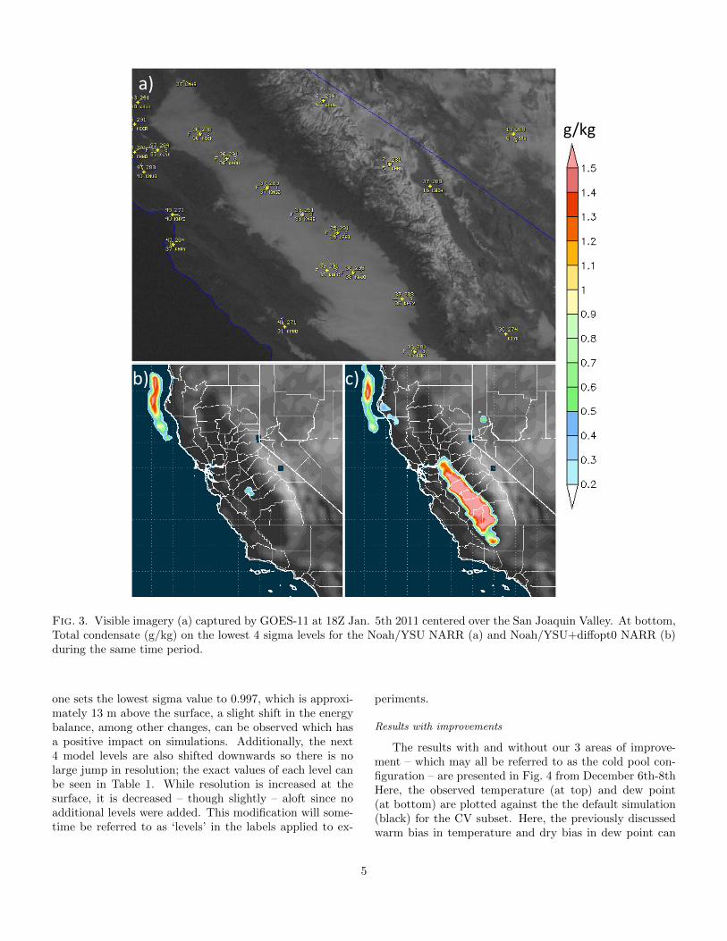
It has been shown that horizontal diffusion operatingalong sigma coordinates can have an impact on forecastingtopographically confined cold pools (Billings et al. 2006;Zangl 2005). However, examining its impact on the CV’sTule fog is important, and to the authors’ knowledge, hasnot been done. A dramatic example of the effects of diffu-sion is presented in Fig. 3. Here, visible satellite imagery(Fig. 3a) shows the Tule fog encompassing the entire SanJoaquin Valley at 10am local time January 5th 2011.

This is compared to the total modeled condensate (g/kg)in the lowest 4 sigma levels for the Noah/YSU NARR(Fig. 3b). One can observe that almost no fog is presentin the simulation that has diffusion operating on modellevels; however, when diffusion is turn off – abbreviated asNoah/YSU+diffopt0 NARR – the problem is fixed (Fig. 3c).This is because when diffusion operates on model levels,which is the default in the WRF model, warmer and drierair from the surrounding mountain ranges is forced downthe slope into the CV. This quickly erodes any fog thatmay have formed and substantially inhibits any future de-velopment. It should be noted that while only a morn-ing snapshot is shown here, this particular Tule fog lastedthroughout the day, which is certainly not uncommon forwinter months. The simulation without diffusion correctlysimulated the fogs persistence.

For this resolution, there is no option currently availablein the WRF model that has diffusion operating in physicalspace. This is a problem due to the fact that high profileweather events such as fog and freezing rain may go com-pletely undetected. It has been suggested and discussedthat WRF even add a simple diffusion option that oper-ates on model levels, but becomes inactive as grid pointsapproach sloping terrain. As of now this has not been im-plemented, but it is agreed that the second best optionwould be to deactivate horizontal diffusion completely.

Billings et al. (2006) noted that increasing the horizon-tal resolution could produce results similar to lower reso-lution runs that had diffusion calculated on model levels.Testing this in the Tule fog case revealed that 4km hori-zontal resolution runs with diffusion on, had results simi-lar to that of 12km with no diffusion. However, increasing

the horizontal resolution to account for the limitations ofdiffusion in the WRF model is not a practical solution, es-pecially because of the increased computation cost. Manyparts of the Southern San Joaquin Valley approach or evenexceed 100km in width, meaning at 12km horizontal resolu-tion, the 8 grid points resolving the valley are insufficientfor diffusion calculated on model levels. If one considersthat most valleys in the Western United States are sub-stantially smaller than the CV, increased resolution willalways result in unresolved features that could be resolvedif diffusion was handled properly. So as previously stated,increased resolution is not the solution, but a way to maskdiffusion errors when calculated on sigma levels.

Reverting back to our December 2005 case, particularlythe 5th-8th, one can find the average overnight (12Z) rela-tive humidity in the Central Valley is around 87% (Fig. 2).This is compared to our NARR and HRLDAS initializedsoils which had a relative humidity of 58 and 54%, respec-tively (Fig. 2). Now, deactivating diffusion and rerunningsimulations results in an 11% increase in overnight relativehumidity. Certainly a large improvement, but values stillseveral standard deviations away from the observed mean.While deactivating diffusion can improve forecasts for cer-tain events, like the January 2011 Tule fog, it is not a cureall and additional modifications need to be explored.

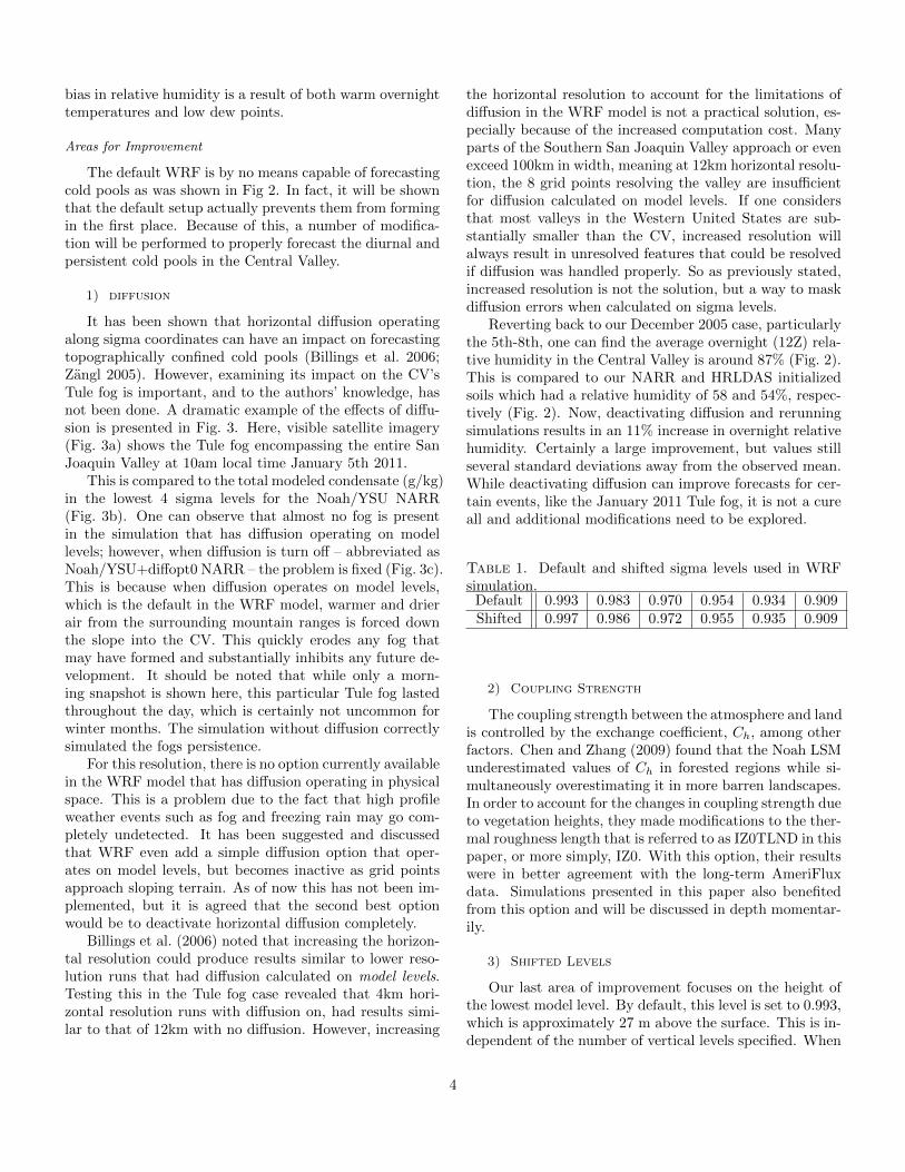
Table 1. Default and shifted sigma levels used in WRFsimulation.

Default 0.993 0.983 0.970 0.954 0.934 0.909Shifted 0.997 0.986 0.972 0.955 0.935 0.909

2) Coupling Strength

The coupling strength between the atmosphere and landis controlled by the exchange coefficient, Ch, among otherfactors. Chen and Zhang (2009) found that the Noah LSMunderestimated values of Ch in forested regions while si-multaneously overestimating it in more barren landscapes.In order to account for the changes in coupling strength dueto vegetation heights, they made modifications to the ther-mal roughness length that is referred to as IZ0TLND in thispaper, or more simply, IZ0. With this option, their resultswere in better agreement with the long-term AmeriFluxdata. Simulations presented in this paper also benefitedfrom this option and will be discussed in depth momentar-ily.

3) Shifted Levels

Our last area of improvement focuses on the height ofthe lowest model level. By default, this level is set to 0.993,which is approximately 27 m above the surface. This is in-dependent of the number of vertical levels specified. When

4

a)

b) c)

g/kg

Fig. 3. Visible imagery (a) captured by GOES-11 at 18Z Jan. 5th 2011 centered over the San Joaquin Valley. At bottom,Total condensate (g/kg) on the lowest 4 sigma levels for the Noah/YSU NARR (a) and Noah/YSU+diffopt0 NARR (b)during the same time period.

one sets the lowest sigma value to 0.997, which is approxi-mately 13 m above the surface, a slight shift in the energybalance, among other changes, can be observed which hasa positive impact on simulations. Additionally, the next4 model levels are also shifted downwards so there is nolarge jump in resolution; the exact values of each level canbe seen in Table 1. While resolution is increased at thesurface, it is decreased – though slightly – aloft since noadditional levels were added. This modification will some-time be referred to as ‘levels’ in the labels applied to ex-

periments.

Results with improvements

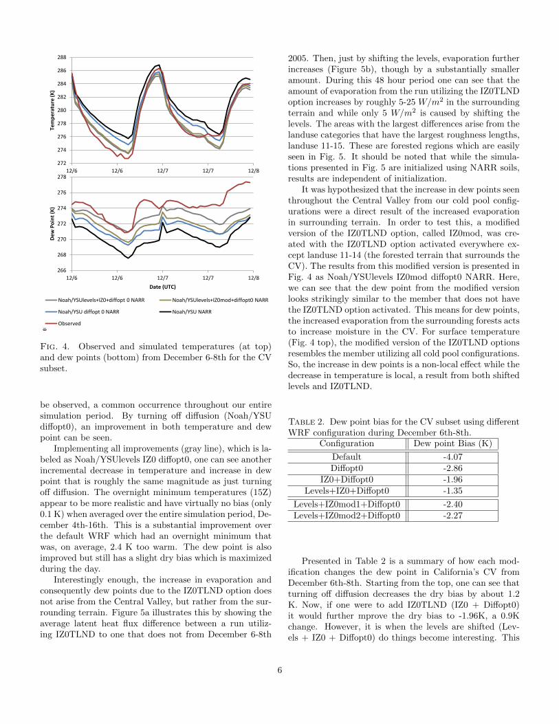
The results with and without our 3 areas of improve-ment – which may all be referred to as the cold pool con-figuration – are presented in Fig. 4 from December 6th-8thHere, the observed temperature (at top) and dew point(at bottom) are plotted against the the default simulation(black) for the CV subset. Here, the previously discussedwarm bias in temperature and dry bias in dew point can

5

272

274

276

278

280

282

284

286

288

12/6 12/6 12/7 12/7 12/8

Tem

pe

ratu

re (

K)

266

268

270

272

274

276

278

12/6 12/6 12/7 12/7 12/8

De

w P

oin

t (K

)

Date (UTC)

Noah/YSUlevels+IZ0+diffopt 0 NARR Noah/YSUlevels+IZ0mod+diffopt0 NARR

Noah/YSU diffopt 0 NARR Noah/YSU NARR

Observed

Fig. 4. Observed and simulated temperatures (at top)and dew points (bottom) from December 6-8th for the CVsubset.

be observed, a common occurrence throughout our entiresimulation period. By turning off diffusion (Noah/YSUdiffopt0), an improvement in both temperature and dewpoint can be seen.

Implementing all improvements (gray line), which is la-beled as Noah/YSUlevels IZ0 diffopt0, one can see anotherincremental decrease in temperature and increase in dewpoint that is roughly the same magnitude as just turningoff diffusion. The overnight minimum temperatures (15Z)appear to be more realistic and have virtually no bias (only0.1 K) when averaged over the entire simulation period, De-cember 4th-16th. This is a substantial improvement overthe default WRF which had an overnight minimum thatwas, on average, 2.4 K too warm. The dew point is alsoimproved but still has a slight dry bias which is maximizedduring the day.

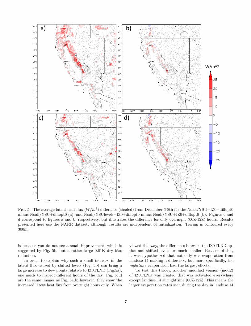
Interestingly enough, the increase in evaporation andconsequently dew points due to the IZ0TLND option doesnot arise from the Central Valley, but rather from the sur-rounding terrain. Figure 5a illustrates this by showing theaverage latent heat flux difference between a run utiliz-ing IZ0TLND to one that does not from December 6-8th

2005. Then, just by shifting the levels, evaporation furtherincreases (Figure 5b), though by a substantially smalleramount. During this 48 hour period one can see that theamount of evaporation from the run utilizing the IZ0TLNDoption increases by roughly 5-25 W/m2 in the surroundingterrain and while only 5 W/m2 is caused by shifting thelevels. The areas with the largest differences arise from thelanduse categories that have the largest roughness lengths,landuse 11-15. These are forested regions which are easilyseen in Fig. 5. It should be noted that while the simula-tions presented in Fig. 5 are initialized using NARR soils,results are independent of initialization.

It was hypothesized that the increase in dew points seenthroughout the Central Valley from our cold pool config-urations were a direct result of the increased evaporationin surrounding terrain. In order to test this, a modifiedversion of the IZ0TLND option, called IZ0mod, was cre-ated with the IZ0TLND option activated everywhere ex-cept landuse 11-14 (the forested terrain that surrounds theCV). The results from this modified version is presented inFig. 4 as Noah/YSUlevels IZ0mod diffopt0 NARR. Here,we can see that the dew point from the modified versionlooks strikingly similar to the member that does not havethe IZ0TLND option activated. This means for dew points,the increased evaporation from the surrounding forests actsto increase moisture in the CV. For surface temperature(Fig. 4 top), the modified version of the IZ0TLND optionsresembles the member utilizing all cold pool configurations.So, the increase in dew points is a non-local effect while thedecrease in temperature is local, a result from both shiftedlevels and IZ0TLND.

Table 2. Dew point bias for the CV subset using differentWRF configuration during December 6th-8th.

Configuration Dew point Bias (K)

Default -4.07Diffopt0 -2.86

IZ0+Diffopt0 -1.96Levels+IZ0+Diffopt0 -1.35

Levels+IZ0mod1+Diffopt0 -2.40Levels+IZ0mod2+Diffopt0 -2.27

Presented in Table 2 is a summary of how each mod-ification changes the dew point in California’s CV fromDecember 6th-8th. Starting from the top, one can see thatturning off diffusion decreases the dry bias by about 1.2K. Now, if one were to add IZ0TLND (IZ0 + Diffopt0)it would further mprove the dry bias to -1.96K, a 0.9Kchange. However, it is when the levels are shifted (Lev-els + IZ0 + Diffopt0) do things become interesting. This

6

W/m^2

a) b)

c) d)

Fig. 5. The average latent heat flux (W/m2) difference (shaded) from December 6-8th for the Noah/YSU+IZ0+diffopt0minus Noah/YSU+diffopt0 (a), and Noah/YSUlevels+IZ0+diffopt0 minus Noah/YSU+IZ0+diffopt0 (b). Figures c andd correspond to figures a and b, respectively, but illustrates the difference for only overnight (00Z-12Z) hours. Resultspresented here use the NARR dataset, although, results are independent of initialization. Terrain is contoured every300m.

is because you do not see a small improvement, which issuggested by Fig. 5b, but a rather large 0.61K dry biasreduction.

In order to explain why such a small increase in thelatent flux caused by shifted levels (Fig. 5b) can bring alarge increase to dew points relative to IZ0TLND (Fig.5a),one needs to inspect different hours of the day. Fig. 5c,dare the same images as Fig. 5a,b; however, they show theincreased latent heat flux from overnight hours only. When

viewed this way, the differences between the IZ0TLND op-tion and shifted levels are much smaller. Because of this,it was hypothesized that not only was evaporation fromlanduse 14 making a difference, but more specifically, thenighttime evaporation had the largest effects.

To test this theory, another modified version (mod2)of IZ0TLND was created that was activated everywhereexcept landuse 14 at nighttime (00Z-12Z). This means thelarger evaporation rates seen during the day in landuse 14

7

* Results independent of soil initialization.

Change in average (Dec. 4-16th) latent heat flux (12Z only)

• Online simulations (using diff_opt=0, IZ0TLND, and shifted levels) do not evaporate as much as offline (IZ0 activated) simulations at 12Z

W/m^2

Fig. 6. The average latent heat flux difference betweenthe Noah/YSUlevels + IZ0 + diffopt0 NARR and offlineHRLDAS (with IZ0TLND activated) at 12Z from Decem-ber 4th-16th

would still exist but the nighttime values would reflect thatof the default WRF. This version is compared to mod1(Table 2) which had IZ0TLND implemented everywherebut landuse 14. Here, one can observe that by allowingmore evaporation during the daytime but not at night, thedry dew points bias was reduced by a mere 0.13K to -2.27K.If the daytime evaporation made the difference, one wouldexpect to see a dew point bias of -1.35K (Levels + IZ0 +Diffopt0) or of similar magnitude.

The cold pool modifications presented here increase evap-oration to mitigate the dry bias, but this may not be con-sistent with offline simulations. Simply put, is it possibleto evaporate more water in the online simulations whilethe offline model evaporates less. So by reinitializing themodel every other day, which is done here, evaporationcould be inconsistent and wouldn’t be an appropriate fixfor modeling cold pools.

To demonstrate the consistency between the online/offlinemodel, Fig. 6 shows the average latent heat flux differ-ence at 12Z from December 4th-16th between an online(Noah/YSUlevel+IZ0+diffopt0 NARR) and offline (HRL-DAS with IZ0 activated) simulation. Here, cooler colorsrepresent less evaporation from the online simulation whilewarmer colors represent more. One can observe that themajority of places surrounding the CV have too little evap-oration relative to the offline model. This means that everytime the model is reinitialized, places shaded in blue end

up losing soil water that should have evaporated into theatmosphere. Of course, the offline model is not necessarilycorrect, but it is concerning to see such large inconsisten-cies between online/offline simulations.

The results presented in Fig. 6 are an average at 12Zbecause the nighttime evaporation was found to be of largeimportance. However, if one inspects the 24 hour average,not much difference is observed. Figure 6 also shows theNARR relative to the HRLDAS; this was done because theNARR had the largest overnight evaporate rates in landuse14, owing to its high soil moisture content in this area. Thismeans the ERA, NAM, and spun soil underestimated theevaporate rates even more.

When the IZ0TLND option is activated in the WRFmodel, technically one should re-spin the soil to accountfor the changes in the exchange coefficient, however; thishas been deemed not necessary and can be explained in thefollowing example. Two simulations were made using thesame physics (Noah/YSUlevels IZ0 diffopt0) but with dif-ferent soil initialization, one spun, and another spun withIZ0TLND activated. Because IZ0TLND was activated of-fline, the December 6-8th dew point bias shifted by 0.23 Kin the full domain while the CV change was only 0.17 K.This difference may be important for some applications,but we find it irrelevant. Because of this small differ-ence, we activated the IZ0TLND option online without re-spinning the soils offline. In addition to this, the other soildatasets (NAM, NARR, ERA) do not provide this option.However, it should be kept in mind that re-spinning thesoils is the proper technique, and would change our resultsby the small magnitude mentioned above.

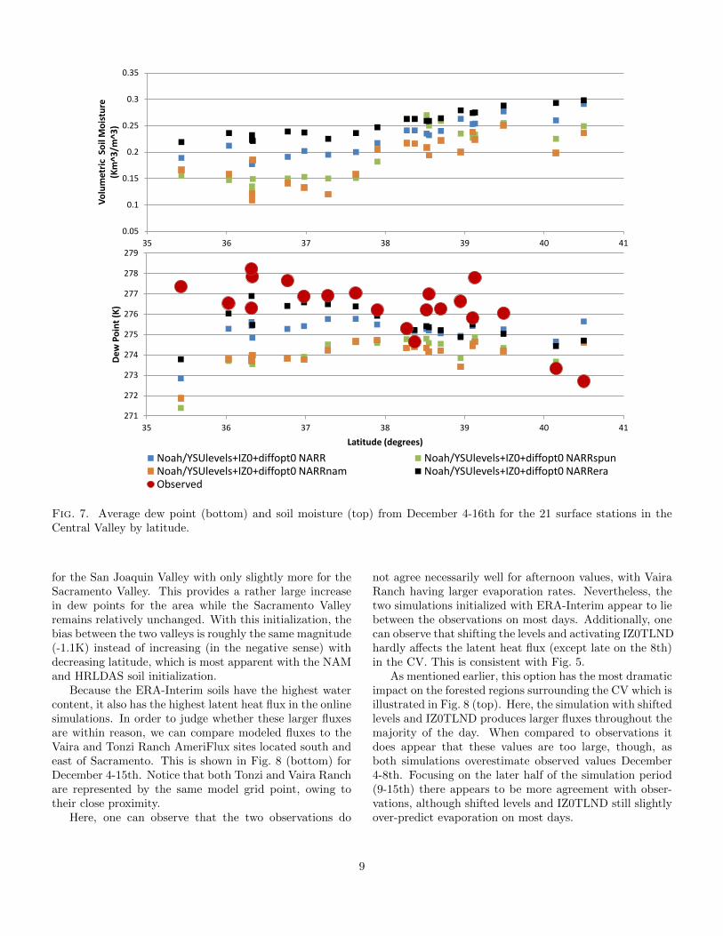
The different soil initialization used in this study havea dramatic range in moisture values, unfortunately. Thisis illustrated in Fig. 7 (top), which shows the average soilmoisture from December 4-16th for the 21 surface station inthe Central Valley by latitude. Here, one can observe thatthe NAM initialized soils (NARRnam) are actually quitesimilar to the ones spun offline in the HRLDAS. However,when one compares the average simulated dew points forthat same time period (Fig. 7 bottom), the dry bias stillpersists, especially in the San Joaquin Valley. Of course,the bias would be much worse (Fig. 4) if the cold poolconfigurations were not utilized.

Even higher moisture content can be seen in the NARRinitialized soils. Consequently, the average dew points arealso higher, although still too dry. This is the case for allstations except in the northern fringe of the SacramentoValley where a shallow moist layer had trouble mixingout. For these two stations (KRDD, KRBL), modeled dewpoints were similar to the rest of the valley, although, ob-servations show that KRDD and KRBL are on average,drier.

Finally, the simulations initialized with ERA-Interimsoils, labeled NARRera, provides even more soil moisture

8

271

272

273

274

275

276

277

278

279

35 36 37 38 39 40 41

Dew

Po

int

(K)

Latitude (degrees)

0.05

0.1

0.15

0.2

0.25

0.3

0.35

35 36 37 38 39 40 41

Vo

lum

etri

c S

oil

Mo

istu

re

(Km

^3/m

^3)

Noah/YSUlevels+IZ0+diffopt0 NARR Noah/YSUlevels+IZ0+diffopt0 NARRspun Noah/YSUlevels+IZ0+diffopt0 NARRnam Noah/YSUlevels+IZ0+diffopt0 NARRera Observed

Fig. 7. Average dew point (bottom) and soil moisture (top) from December 4-16th for the 21 surface stations in theCentral Valley by latitude.

for the San Joaquin Valley with only slightly more for theSacramento Valley. This provides a rather large increasein dew points for the area while the Sacramento Valleyremains relatively unchanged. With this initialization, thebias between the two valleys is roughly the same magnitude(-1.1K) instead of increasing (in the negative sense) withdecreasing latitude, which is most apparent with the NAMand HRLDAS soil initialization.

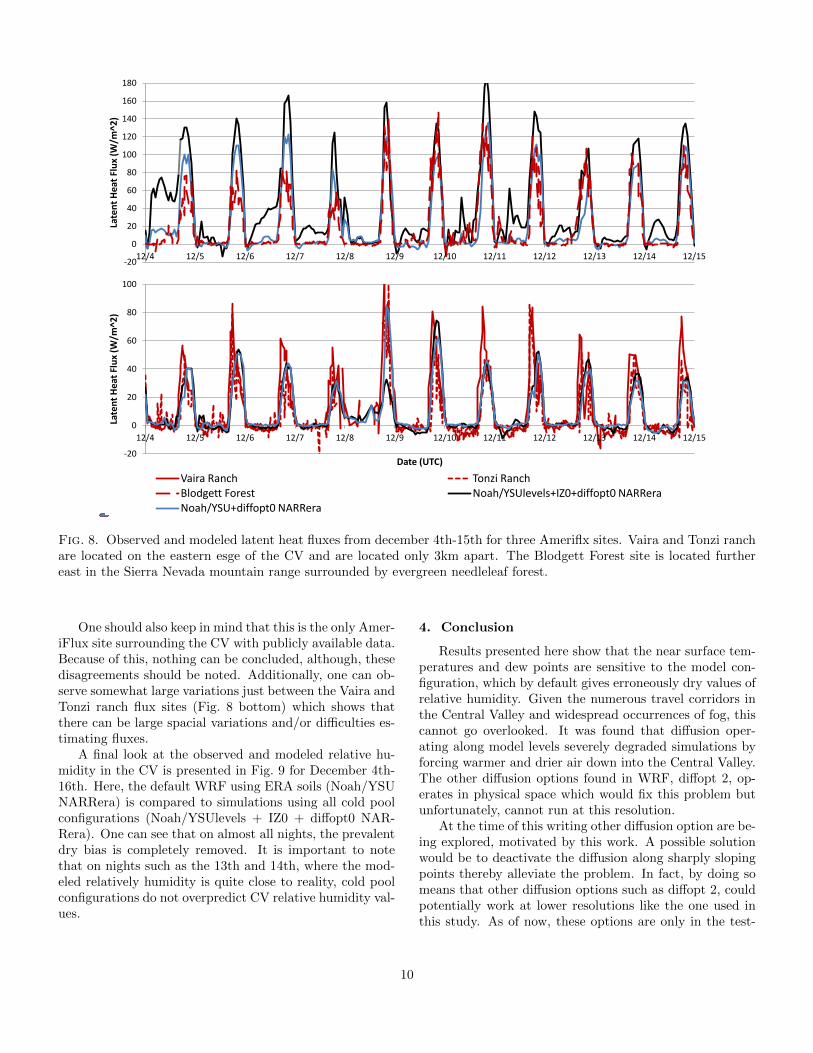
Because the ERA-Interim soils have the highest watercontent, it also has the highest latent heat flux in the onlinesimulations. In order to judge whether these larger fluxesare within reason, we can compare modeled fluxes to theVaira and Tonzi Ranch AmeriFlux sites located south andeast of Sacramento. This is shown in Fig. 8 (bottom) forDecember 4-15th. Notice that both Tonzi and Vaira Ranchare represented by the same model grid point, owing totheir close proximity.

Here, one can observe that the two observations do

not agree necessarily well for afternoon values, with VairaRanch having larger evaporation rates. Nevertheless, thetwo simulations initialized with ERA-Interim appear to liebetween the observations on most days. Additionally, onecan observe that shifting the levels and activating IZ0TLNDhardly affects the latent heat flux (except late on the 8th)in the CV. This is consistent with Fig. 5.

As mentioned earlier, this option has the most dramaticimpact on the forested regions surrounding the CV which isillustrated in Fig. 8 (top). Here, the simulation with shiftedlevels and IZ0TLND produces larger fluxes throughout themajority of the day. When compared to observations itdoes appear that these values are too large, though, asboth simulations overestimate observed values December4-8th. Focusing on the later half of the simulation period(9-15th) there appears to be more agreement with obser-vations, although shifted levels and IZ0TLND still slightlyover-predict evaporation on most days.

9

-20

0

20

40

60

80

100

12/4 12/5 12/6 12/7 12/8 12/9 12/10 12/11 12/12 12/13 12/14 12/15

Late

nt

Hea

t Fl

ux

(W/m

^2)

Date (UTC)

-20

0

20

40

60

80

100

120

140

160

180

12/4 12/5 12/6 12/7 12/8 12/9 12/10 12/11 12/12 12/13 12/14 12/15

Late

nt

Hea

t Fl

ux

(W/m

^2)

Vaira Ranch Tonzi Ranch Blodgett Forest Noah/YSUlevels+IZ0+diffopt0 NARRera Noah/YSU+diffopt0 NARRera

Fig. 8. Observed and modeled latent heat fluxes from december 4th-15th for three Ameriflx sites. Vaira and Tonzi ranchare located on the eastern esge of the CV and are located only 3km apart. The Blodgett Forest site is located furthereast in the Sierra Nevada mountain range surrounded by evergreen needleleaf forest.

One should also keep in mind that this is the only Amer-iFlux site surrounding the CV with publicly available data.Because of this, nothing can be concluded, although, thesedisagreements should be noted. Additionally, one can ob-serve somewhat large variations just between the Vaira andTonzi ranch flux sites (Fig. 8 bottom) which shows thatthere can be large spacial variations and/or difficulties es-timating fluxes.

A final look at the observed and modeled relative hu-midity in the CV is presented in Fig. 9 for December 4th-16th. Here, the default WRF using ERA soils (Noah/YSUNARRera) is compared to simulations using all cold poolconfigurations (Noah/YSUlevels + IZ0 + diffopt0 NAR-Rera). One can see that on almost all nights, the prevalentdry bias is completely removed. It is important to notethat on nights such as the 13th and 14th, where the mod-eled relatively humidity is quite close to reality, cold poolconfigurations do not overpredict CV relative humidity val-ues.

4. Conclusion

Results presented here show that the near surface tem-peratures and dew points are sensitive to the model con-figuration, which by default gives erroneously dry values ofrelative humidity. Given the numerous travel corridors inthe Central Valley and widespread occurrences of fog, thiscannot go overlooked. It was found that diffusion oper-ating along model levels severely degraded simulations byforcing warmer and drier air down into the Central Valley.The other diffusion options found in WRF, diffopt 2, op-erates in physical space which would fix this problem butunfortunately, cannot run at this resolution.

At the time of this writing other diffusion option are be-ing explored, motivated by this work. A possible solutionwould be to deactivate the diffusion along sharply slopingpoints thereby alleviate the problem. In fact, by doing someans that other diffusion options such as diffopt 2, couldpotentially work at lower resolutions like the one used inthis study. As of now, these options are only in the test-

10

20

30

40

50

60

70

80

90

100

12/4 12/5 12/6 12/7 12/8 12/9 12/10 12/11 12/12 12/13 12/14 12/15 12/16

Rel

ativ

e H

um

idit

y (%

)

Date (UTC)

Noah/YSU NARRera Noah/YSU+diffopt0 NARRera Noah/YSUlevels+IZ0+diffopt0 NARRera Observed

Fig. 9. Observed and modeled relative humidity for the CV subset (Fig. 1) from December 4-16th 2005. Plus or minusone standard deviation for observed RH is shown every third hour.

ing phase so the next best solution would be to deactivatediffusion completely.

Furthermore, it was found that shifting the default ver-tical levels and activating the IZ0TLND option could fur-ther improve the dry relative humidity bias. It was foundthat small shifts in the surface energy balance due to theseoptions decreased overnight minimum sensible tempera-tures. Additionally, these options acted to increase theCentral Valley dew points because of increased evaporationin the surrounding forests. While both the day and night-time evaporation increased, only the changes observed innighttime values were of significance. It can be said that allthree cold pool configurations acted to decrease the tem-perature while also increasing dew points.

Additional research is needed to verify that the largerlatent heat flux observed in the forests in the online/offlinesimulations are in fact, realistic. Due to insufficient fluxdata around the CV, verification will require running of-fline simulations in other forested areas and times. Withthat being said, more consistent evaporation rates betweenonline/offline simulations are needed since the online modelalmost always underevaporates. The underlying goal ofspinning models offline is to be consistent, yet consistencywas never achieved here. Understanding the exact reasonswhy is desirable and ongoing.

California’s Central Valley is home to many urbanizedareas which are often plagued by diurnal and persistentcold pools conducive for dense fog. Recommendations pre-sented here bring large improvements which can dramati-cally improve forecasting the non-linear evolution of theseevents.

Acknowledgments.

Support for this project was provided by the Devel-opmental Testbed Center (DTC). The DTC Visitor Pro-gram is funded by the National Oceanic and AtmosphericAdministration, the National Center for Atmospheric Re-search and the National Science Foundation.

The data used in this study were acquired as part ofthe mission of NASA’s Earth Science Division and archivedand distributed by the Goddard Earth Sciences (GES) Dataand Information Services Center (DISC)

REFERENCES

Avery, L., 2011: Challenges of meteorological and photo-chemical modeling of utahs wintertime cold pools. West-ern Meteorological, Emissions, and Air Quality ModelingWorkshop, Boulder, CO.

Baker, K. R., H. Simon, and J. T. Kelly, 2011: Chal-lenges to modeling ”cold pool” meteorology associatedwith high pollution episodes. Environmental Science andTechnology, 45(17), 7118–9.

Billings, B. J., V. Grubisic, and R. D. Borys, 2006: Mainte-nance of a mountain valley cold pool: A numerical study.Monthly Weather Review, 134, 2266–2278.

Bodine, D., P. M. Klein, S. C. Arms, and A. Shapiro, 2009:Variability of surface air temperature over gently sloped

11

terrain. Journal of Applied Meteorology and Climatology,48, 1117–1141.

Chen, F. and Y. Zhang, 2009: On the coupling strengthbetween the land surface and the atmosphere: Fromviewpoint of surface exchange coefficients. Geophys. Res.Lett., 36, L10 404, doi:10.1029/2009GL037 980.

Clements, C. B., C. D. Whiteman, and J. D. Horel, 2003:Cold-air-pool structure and evolution in a mountainbasin: Peter sinks, utah. Journal of Applied Meteorol-ogy, 42, 752–768.

Daly, C., D. Conklin, and M. Unsworth, 2009: Local atmo-spheric decoupling in complex topography alters climatechange impacts. International Journal of Climatology,30, 1857–1864.

Gillies, R. R., S. Wang, and M. R. Booth, 2010: Atmo-spheric scale interaction on wintertime intermountainwest low-level inversions. Weather and Forecasting, 25,1196–1210.

Gudiksen, P. H., J. M. L. Jr., C. W. King, D. Ruffieux,and W. D. Neff, 1992: Measurements and modeling ofthe effects of ambient meteorology on nocturnal drainageflows. Journal of Applied Meteorology, 31, 1023–1032.

Gustavsson, T., M. Karlsson, J. Bogren, and S. Lindqvist,1998: Development of temperature patterns during clearnights. Journal of Applied Meteorology, 37, 559–571.

Hootman, B. W. and W. Blumen, 1983: Analysis of night-time drainage winds in boulder, colorado during 1980.Monthly Weather Review, 111, 1052–1061.

Hunt, E. D., J. B. Basara, and C. R. Morgan, 2007: Signif-icant inversions and rapid in situ cooling at a well-sitedoklahoma mesonet station. 46, 353–367.

Katurji, M. and S. Zhong, 2012: The influence of topogra-phy and ambient stability on the characteristics of cold-air pools: a numerical investigation. Journal of AppliedMeteorology and Climatology, 51, 1740–1749.

LeMone, M. A., K. Ikeda, R. L. Grossman, and M. W. Ro-tach, 2003: Horizontal variability of 2-m temperature atnight during cases-97. Journal of the Atmospheric Sci-ences, 60, 2431–2449.

Mahrt, D. Vickers, R. Nakamura, M. R. Soler, J. L. Sun,S. Burns, and D. H. Lenschow, 2001: Shallow drainageflows. Boundary Layer Meteorology, 101, 243260.

Neff, W. D. and C. W. King, 1989: The accumulation andpooling of drainage flows in a large basin. Journal ofApplied Meteorology, 28, 518–529.

Ryerson, W. R., 2012: Toward improving short-rangefog prediction in data-denied areas using the air forceweather agency mesoscale ensemble. Ph.D. thesis, NavalPostgraduate School, Monterey, California.

Thompson, B. W., 1986: Small-scale katabatics and coldhollows. Weather, 41, 146153.

Whiteman, C. D., 2000: Mountain Meteorology. OxfordUniversity Press, 355 pp.

Whiteman, C. D., T. Haiden, B. Pospichal, S. Eisenbach,and R. Steinacker, 2004: Minimum temperatures, diur-nal temperature ranges, and temperature inversions inlimestone sinkholes of different sizes and shapes. Jour-nal of Applied Meteorology, 43, 1224–1236.

Whiteman, C. D., T. B. McKee, and J. C. Doran, 1996:Boundary layer evolution within a canyonland basin.part i: Mass, heat, and moisture budgets from obser-vations. Journal of Applied Meteorology, 35, 2145–2161.

Whiteman, C. D., S. Zhong, W. J. Shaw, J. M. Hubbe,X. Bian, and J. Mittelstadt, 2001: Cold pools in thecolumbia basin. Weather and Forecasting, 16, 432–447.

Zangl, G., 2005: Formation of extreme cold-air pools inelevated sinkholes: An idealized numerical process study.Monthly Weather Review, 133, 925–941.

Zhong, S. C., D. Whiteman, X. Bian, W. J. Shaw, andJ. M. Hubbe, 2001: Meteorological processes affect-ing the evolution of a wintertime cold air pool in thecolumbia basin. Monthly Weather Review, 129, 2600–2613.

12