model-free forecasting for nonlinear time series (with application to exchange rates)

Computational Statistics & Data Analysis 19 (1995) 433-459 North-Holland

433

Model-free forecasting for nonlinear time series ( with application to exchange rates)

Berlin Wu Department of Mathematical Sciences, National Chengchi Uniuersity, Taipei, Taiwan

Received June 1993 Revised October 1993

Abstract: The first step in nonlinear model construction is data identification. While the major drawback with most of the nonlinear tests is that they are designed to test a parametric null against certain parametric alternatives and are therefore inconsistent against all possibile alternatives. In this Paper, by incorporating the neurocomputing technique, the intriguing model construction and forecast Problems such as how to find a best fitted model and to obtain a more appropriate prediction Performance are addressed. The dynamic abilities of this approach lies in the fact that the multilier feed forward networks are functional approximators for any functions. Simulations verify that the neural networks perform a robust forecast for some nonlinear time series. Finally, we use the data of the exchange rates of Taiwan to compare the predictive performances of neural networks with ARIMA models.

Keywords: Model-free forecasting; Neural networks; Back-propagation method; Bilinear models; Exchange rates.

1. Introduction

To exhibit the empirical data in an appropriate model in the application of nonlinear time series, researchers in this field have been concerned with the nonlinear System such as bilinear models (Granger and Anderson, 1978; Subba Rao and Gabr, 1984), threshold autoregressive models (Tang and Lim, 19801, state-dependent models (Priestley, 19801, autoregressive models with conditional heteroscedasticity (Engle, 19821, autoregressive models with discrete state space (McKenzie, 1985) and doubly stochastic models (Tjostheim, 1986). Their works draw lights on closer understanding of the nonlinear phenomena underlying the data (c.f. De Gooijer and Kumar, 1992). However, these works are complicated issues, solutions to some of which have eluded us even in the case of linear models, and promise to be far more complicated when we enter the realm of nonlinear dynamic models, see Granger (1991) and Pesaran and Potter (1992).

Correspondence to: Dr. B. Wu, Institute of Mathematical Science, National Chengchi University, Wen-Shen District, Taipei, Taiwan, Rep. of China.

0167-9473/95/$09.50 0 1995 - Elsevier Science B.V. All rights reserved SSDI 0167-9473(94)00008-7

434 B. Wu / Robust forecasting

On the other hand, the results obtained so far do not provide an efficient rule in testing whether the correct nonlinear specification has been achieved or there still remains some neglective nonlinearity in the estimated relationship. Since uncertainties usually exist for the correct underlying parametric models, the dynamic form, lag structure and the stochastic assumptions heavily impact the power of the tests and the forecast Performance. Therefore to propose a model-free for forecasting nonlinear time series is what we most concerned.

The Problem of classifying nonlinear time series tan be divided into two groups: model-based and model-free Systems. Most of the former work to date has relied on diagnoses such as Lagrange Multiplier (LM) test (Weiss, 1986; Luukkonen et al, 1988; Saikkonen and Luukkonen, 1988; Guegan and Pham, 19921, Bispectrum test (Hinich, 1982), Likelihood ratio-based tests (Chan and Tong, 1986) and so forth. Unfortunately, these available methods were based on a particular class of nonlinear time series models and none of the above tests with reasonable power tan dominate the others. For instance, the LM test is designed to reveal specific types of nonlinearity. The test may also have some power against incorrect alternatives. There may sometimes exist alternative nonlinear models against which the LM test is not powerful. Hence, rejecting the null hypothesis on the basis of this test will have not very strong conclusions for the type of possible nonlinearity.

More recently, the widespread applications of artificial neural networks have received a huge impact on the research of nonlinear Systems. Researchers in neurocomputing use feedward networks, e.g. Lapedes and Farber (1987); Kosoko (1991); to predict future values of time series only by extracting knowledge from the past. This is an area of considerable applications due to its potential for providing insights into the kind of highly parallel computation. Since neural networks are the universal approximators for the unknown functions, no assumptions should be hypothesized for the data set. That is, no Prior models are built for the unknown functions. This characteristic is quite different from the traditional linear models or any other specific nonlinear models, such as the time series which is assumed to be linear and stationary in ARIMA models. Therefore the special capability of neural networks has made themselves a suitable analysis tool for various Patterns of time series.

The goal of this Paper is to propose a neurocomputing technique to perform the robust forecasting for some nonlinear time series. The robust properties for forecasting Performance will be discussed by comparing with other model-based procedures.

2. Neural networks and model-free forecast

2.1. Motivation for forecasting of nonlinear time series

Among the nonlinear models, the bilinear model is regarded as the most natura1 and simplest one that tan represent the series much better than linear

B. Wu / Robust forecasting 435

models. In fact, Brockett (1976) has shown that the bilinear model tan approximate to an arbitrary degree of accuracy Volterra series relationship over a finite time interval if the model Parameters are properly Chosen. A special feature which is worth mentioning here is that the bilinear models are especially suitable to exhibit the suddenly burst data with very large amplitude in extraor- dinary periods. The general bilinear models first proposed by Granger and Anderson (1978) took the form

XI + 2 aiX*_i= c CjE,_j + E t bijXr_iet-j, i=l j=O i=l j=l

(24

where c. = 1 and {et} is a stritt white noise process with zero mean and finite variance uET, and the ai, bij and cj are constants. We often denote (2.1) as BUP, r, m, k).

Granger and Anderson (1978) noticed that some simple bilinear series have zero second Order autocorrelation and might be mistaken as white noise or an ARIMA model with higher orders. Subba Rao and Gabr (1984) have proposed a method about model identification and Parameter estimation of BL(p, 0, m, n). But it takes a lot of computations and iterations. Wu and Shih (1992) suggested a more efficient process than Subba Rao and Gabr’s method for simple bilinear models. However, for the bilinear time series, there are still no consistent and efficient methods in identification Problem at present. Not even to say about the forecast of bilinear models.

Fortunately the imlementation abilities of estimating, testing, modeling, forecasting and controlling the underlying System for neural networks will provide great incentive. The methodology of research tan be outlined by the following procedures: (a) construct the adequate neural System (b) data pre-processing procedure (c) networks initialization (d) training (e) forecasting.

2.2. The architecture of multilayer feedforward neural networks

Recent developments in neural networks theory (Lapedes and Farber, 1988, Grosberg, 1988; Cybento, 1989; Funahashi, 1989; Hecht-Nielsen, 1989; Kolen and Goel, 1991; and Kosko, 1992) have shown that the multilayer feedforward neural networks with one hidden layer of neurons tan be used to approximate any Borel-measurable functions to any desired accuracy. The basic idea here is that if the nonlinear laws tan govern the System, even the dynamic behavior is chaotic, the future in some extent may be predicted by the behavior of the past values. The learning is carried out by iteratively adjusting the linking weights in the network so as to minimize the differentes between the actual output vector of the network and the target vector.

In the learning process, an input vector is presented to the network and propagated forward to determine the output Single. The output vector is then compared with the target output vector through the network in Order to adjust the linking weights. This learning process is repeated until the network responds for each input vector with an output vector that is sufficiently close to the


output layer

hidden layer

input layer

XI X2 ‘Ni

I\

’ : bias .I

Fig. 1. A three-layer feedforward network.

desired one. We now consider a three-layer (one for input, one for hidden and one for output) network, as shown in Figure 1.

The general formula for the activation A of each unit in the network (except for the input vector whose activation is clamped by the input vector) is given by:

N Aj(W, a) = s c wjiai >

i 1 i=o (2.2)

where wji is the linking weights between unit j (for which the activation is calculated) and unit i in the next lower layer, N is the total number of units in that layer, ai is the activation of unit i, ao is an input that always has the value 1, and w$ is the threshold or bias for unit j and S is the Sigmoid function as equation (2.3)

S(X) = (1 + e-“)-‘.

Thus, the activation of a hidden unit, (2.3)

hj =AJv; x) = S (2.4)

where v represents the linking weights between layer x and h and vjo is the bias of, hidden unit j, x. is an input that always has the value 1, h, is a constant output equal to 1, and Ni is the number of nodes in the input layer. The activation of an output unit,


where w represents the strength of the couplings between layer h and o, and wjo is the bias of output unit j, h, now become an input that always has the value 1, and Nh is the number of nodes in hidden layer. The total error of the Performance of the network, E, is defined as:

E = i Z C (Oj,c -Yj,c)*, (2.6) c=l j=l

where c runs over all cases (input vectors with their corresponding target output vectors), N, is the total number of cases, oj is the actual value (activation) of output unit j, given the input vector, N, is the total number of output units, and yj is the target value of unit j. To minimize E, each linking weight is updated by an amount proportional to the partial derivative of E with respect to that coupling (accumulated over all cases).

Since the partial derivative of E with respect to wji is

aE aE aoj -=-- awji ao, awji ’ (2.7)

where

aE - =Oj -Yj,

aoj

and

30, aw.. = oj(l - oj)hi.

11

Hence we have

E = (oj -yj)oj(l - oj)hi.

On the other hand, the partial derivative of E with respect to Vik is

where

ao, - =Oj(l -Oj)Wji, ahi

and

(2.8)

P9

(2.10)

(2.11)

(2.12)

(2.13) ah,

- =yi(l -yi)xk. avik


We have

; = 2 (Oj-yi)oj(l-oj)wjihi(l-h,)xk. lk j=l

(2.14)

The linking weights wji are updated according to the following rule (c.f. Rumelhart et al., 1986; and Voglet et al., 1988):

Awji(t + 1) = -[

and the coupling strengths uik are updated as:

(2.15)

(2.16)

where t represents the epoch or sweep number (i.e., the number of times the network has been through the whole set of cases, at which time the linking weights are updated), c runs over cases, N, is the total number of cases. .$ is the learning rate, (Y is the relative contribution of the previous Change of the coupling strength (CZ is the so called momentum factor). The back-propagation algorithm amounts to performing gradient descent on a hyper surface in coupling strength space, where at any Point in that space the error of performance (2.6) is the height of the surface.

Note that we use the mean squared error in stead of E in (2.6) to measure the Performance of a trained networks, and stop the training processes if the mean squared error is less than 0.05.

2.3. Neural network us a model-free predictor

A neural network’s topology and dynamics define a black-box approximator from input to output. The unknown function f : X + Y produces the observed Sample Pattern pairs (X,, Y,), (X,, Y,>, <X,, Y,), . . . . The Sample data modify Parameters in the neural estimator and bring the neural system’s input-output responses closer to the input-output responses of the unknown estimate f. In psychological terms, the neural System learns from experience. In the neural- estimation process, we don’t ask the neural engineer to articulate, write down or guess at the mathematical shape of unknown function f. This is why we called the neural networks estimation as model-free.

Suppose we have just one output unit (i.e. N, = 11, for notational conve- nience, we shall write wli = wi and oi = o. If we Substitute the expression yj in (2.4) into the expression of (2.5), then we have output function activation as a function solely of inputs and weights, as shown in equation (2.17):

(2.17)


The expression f(n, 0) is convenient short-hand for network output since this depends only on inputs and weights. Where the Symbol x represents a vector of all the input values, and the Symbol 8 represents weight matrix (w’s and v’s). We cal1 f the “networks output function”.

In fact, f(x, 0) tan be regarded as a regression curve. According to (2.17) we tan rewrite equation (2.6) as the following form:

E=+ 2 (y,-oc)*=+ 2 (yc-f(X, 0))‘. c=l c=l

(2.18)

Note that the goal of the network learning is to minimize E in (2.18). Thus the network learning proceeding tan be viewed as a “least squared problcm”, which means that to pick a Parameter 8 so that (2.18) tan be minimized. If 0, denotes a Solution of !2.18), then, with the proper mathematical arguments, ‘It tan be proven that BNC tends to t9* (optimal network weights) as N, become large (White, 1981). Thus, back-propagation and nonlinear regression tan be viewed as an alternative statistical approach.

I Begin of a new networks

Step 1 Design the network's layer and nodes

5

Step 2 Initialize weights w, v\

Step 3 Normalization of the data and set up (x,y)

Step 4 Calculate the state of layers

-+ and comput the errors

L

Step 5 Adjust weights of output layer Adjust weights of hidden layer

Step 6

Yes

Fig.2. The flowchart ofthe error back-propagation training.


After the learning process of our network being finished, we tan obtain a solution O* which minimized (2.18). A set of weights 8” yields network output f(xC, 0) that is mean Square optimal for y,; it minimizes expected squared error as a prediction for y,. Of all functions of xC, the best predictor of y, is the conditional expectation E( y, 1 xJ. It turns out that the weights 8” deliver a network that is also a mean Square optimal approximation to the conditional expectation E( y, ) x,).

It is proved by Cybenko (1989) and Funahashi (1989) that f tan approximate any continuous function on a compact set with the uniform topology by a layered network with one hidden layer. Hornik et al. (1989) have also demonstrated that the network output function f(x, 6) tan provide an accurate approximation to any function of x likely to be encountered, providing that Nh, the number of hidden units, is large enough. Because of this “universal approximation” property, hidden layer feedforward networks are useful for application in forecasting.

In practice, it is possible to have excellent fits for training samples, but the application of back-propagation is fraught with difficulties to the forecast Performance on test samples. Unlike most other learning Systems that have been previously discussed, there are far more choices to be made in applying the gradient descent method. Even the slightest Variation tan make the differente between good and bad Performance. While we consider many of these varia- tions, there is no universal answer to what is really best. The major route to get the best results is through repeated experimentation with varying experimental conditions.

Figure 2 illustrates the flowchart of the error back-propagation training algorithm for a basic three-layer network as in Figure 1. Summary of Steps for building a neural network are listed below:

Step 1: Design the network’s layers and nodes. Because the decision of the layers and nodes numbers relies on proper training data, there are no stritt answer for it, Though it has been proved that the neural networks with one hidden layer are sufficient for a function approximator. Sometimes, however, a Problem seems to be more easily solved with more than one hidden layer. It is because an approximator with three layers would require an impractical large number of hidden units. Another question of choosing the hidden neurons’ size is under intensive study (Kosko, 1992 and Wu et al., 1992). The exact analysis is rather difficult because of the complexity of the network mapping and the nondeter- ministic nature of many successfully completed training procedures. The rules for getting the more optimal results are to repeat our experimentation with varying experimental conditions. To sum up, the networks must efficiently integrate the largest possible number of relevant factors. For instance, the AR(p) model used for this type of Problem suggests p for the input number. One output is designed for the neural System to give the predictions. We should note that p is maybe a good Suggestion, but it is possible that p is not the best choice.

B. Wu / Robustforecasting 441

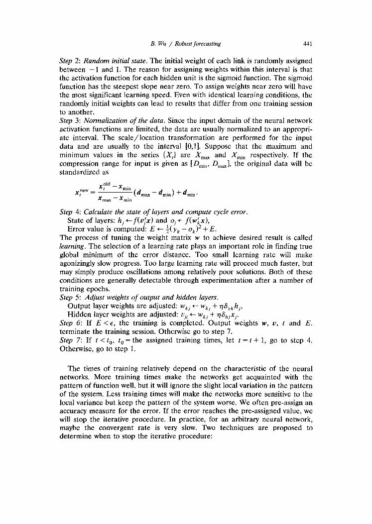
Step 2: Random initial state. The initial weight of each link is randomly assigned between - 1 and 1. The reason for assigning weights within this interval is that the activation function for each hidden unit is the sigmoid function. The sigmoid function has the steepest slope near Zero. To assign weights near zero will have the most significant learning Speed. Even with identical learning conditions, the randomly initial weights tan lead to results that differ from one training Session to another. Step 3: Normalization of the data. Since the input domain of the neural network activation functions are limited, the data are usually normalized to an appropriate interval. The scale/location transformation are performed for the input data and are usually to the interval [O,l]. Suppose that the maximum and minimum values in the series {X,) are X,, and Xmin respectively. If the compression range for input is given as [ Dmin, Dm,], the original data will be standardized as

old qw = xt - Xmin

x - Xmin Cdm= - dmin > + drnin * max

Step 4: Calculate the Stute of layers and compute cycle error. State of layers: h, + f($x) and oj +- f(wLx>, Error value is computed: E + i( yk - o,12 + E.

The process of tuning the weight matrix w to achieve desired result is called Zearning. The selection of a learning rate plays an important role in finding true global minimum of the error distance. Too small learning rate will make agonizingly slow progress. Too large learning rate will proceed much faster, but may simply produce oscillations among relatively poor solutions. Both of these conditions are generally detectable through experimentation after a number of training epochs. Step 5: Adjust weights of output and hidden layers.

Output layer weights are adjusted: wkj +- wkj + r$,,h,, Hidden layer weights are adjusted: uji + wkj + qOhjxj.

Step 6: If E <E, the training is completed. Output weights w, Y, t and E. terminate the training Session. Otherwise go to step 7. Step 7: If t < t,, t, = the assigned training times, let t = t + 1, go to step 4. Otherwise, go to step 1.

The times of training relatively depend on the characteristic of the neural networks. More training times make the networks get acquainted with the Pattern of function well, but it will ignore the slight local Variation in the Pattern of the System. Less training times will make the networks more sensitive to the local variance but keep the Pattern of the System worse. We often pre-assign an accuracy measure for the error. If the error reaches the pre-assigned value, we will stop the iterative procedure. In practice, for an arbitrary neural network, maybe the convergent rate is very slow. Two techniques are proposed to determine when to stop the iterative procedure:


(i) Limit the number of epochs: Training is ceased after a fixed upper limit to the number of training epochs. For instance, when training does not yield a Solution that makes the error near to the zero distance, training could cease after 300 epochs and the link weights would be used as the final Solution.

(ii) Measure the improved progress: The error distance tan be sampled and averaged over a fixed number of epochs, e.g., every 100 epochs of training. If the average error distance for the most recent 100 epochs is not better than that for previous 100, we tan conclude that no progress is made and we should stop training.

After a neural network is properly built, we tan make use of it to forecast the future values by inputting the present data without knowing its specijk model.

3. A Simulation study for bilinear time series

A simulated example. Our research is focused on simple bilinear time series because they often appear in practice and they are widely used in the literature. We selected several bilinear time series as followed:

set 3-1

I

X f+l = 20 + 0.2X,E, + Et+l, X 1+1 = 20 + 0.5X,E, + Er+l, X f+l = 20 + 0.8X,E, + Et+l.

set 3-2

1

X f+l= 20 + 02X*_,E, + EI+l> X I+l= 20 + 0.5X,_,E, + Et+l, X f+1 = 20 + 0.8X,_,E, + E,,l.

set 3-3

1

X f+l= 20 + 0.2X&l+ E,,l, X t+1= 20 + 0.5X*E,_, + E,,l, X t+i = 20 + O.SX*E,_, + Et+l.

set 3-4

I

X t+l = 20 + 0.2x, + 0.2X,E, + Et+l, X 1+1 = 20 + 0.5x, + 0.5X,E, + Et+l, X 1+1 = 20 + o.sx, + O.SX,E, + Et+i.

set 3-5

i

X f+i = 20 + 0.2x, + 0.2X,E, - 0.2X,_1E,_l + Ei+l> X f+i = 20 + 0.5x, + 0.5X,E, - 0.5Xt_1Et_1 + Et+r, X 1+1 = 20 + O.SX, + 0.8X,~, - 0.8X,_i~,_i + E~+~.


Xt-1 XM Xt-3 X-8

Fig. 3. The structure of the established neural nehvorks.

The above series from set 3-l to set 3-5 tan be denoted as BL(0, 0, 1, 11, BL(0, 0, 2, 11, BL(0, 0, 1, 21, BL(1, 0, 1, 1) and BL(1, 0, 2, 21, respectively. As to the tendencies of these bilinear time series, we tan refer to Appendix A. The observations of 518 Sample sizes were obtained by generation, where the innovations E, N N(0, 1). The initial value X, is given as 1.0. The last 10 observations were kept for the comparison of forecasting Performance. Because the bilinear or some other nonlinear models are not well developed to date, we tan hardly fit these bilinear series by some specified nonlinear models. In this simulated study, we try to approximate the nonlinear series by a well developed linear process, Box and Jenkins (1976) method, for the reason that this linear approach has been widely and successfully used in many scientific fields. Hence, we will fit these bilinear series by ARIMA models as the comparative models to neural networks.

Networks initialization According to the procedure stated at Section 2, we design a neural network

whose structure is shown in Figure 3. The initial conditions for the networks are given as followed:

Hidden layers (and neurons): No. of input neurons: No. of output neurons: compression range for the input: compression range for the output: initial (random) weight range:

2 (40 x 401, 8,

[112 21, [O, 1;, [ - 0.1, 0.11,

%

P P

Tabl

e 1

Com

paris

ons

of R

MSE

an

d M

AE

for

the

best

fit

ted

AR

MA

m

odel

s an

d th

e ne

ural

ne

twor

ks

appr

oach

. 3 \

Dat

a se

t 3-

l-l

3-l-2

3-

l-3

3-2-

l 3-

2-2

3-2-

3 3-

3-l

3-3-

2 3-

3-3

3-4-

l 3-

4-2

3-4-

3 3-

5-1

3-5-

2 3-

s-3

*

RM

SE

for

AR

4.

42

12.8

5 32

.12

4.35

11

.62

25.0

0 4.

55

12.6

2 30

.59

5.50

25

.55

171.

38

7.21

30

.76

181.

14

B

2 R

MSE

fo

r N

N

4.37

15

.34

28.8

0 2.

37

10.8

1 19

.26

4.43

12

.63

28.0

8 4.

51

25.6

9 13

0.42

3.

70

24.6

8 17

0.72

6

MA

E fo

r A

R

3.41

8.

90

18.0

8 3.

36

8.55

13

.68

3.47

8.

76

17.6

3 4.

23

16.7

8 76

.66

5.56

22

.75

114.

60

2

MA

E fo

r N

N

3.40

10

.94

18.0

6 1.

83

7.98

13

.49

3.49

8.

88

17.3

9 3.

51

17.3

2 76

.29

2.71

18

.47

109.

07

f: g.

Adv

anta

ge

NN

A

R

NN

N

N

NN

N

N

- A

R

NN

N

N

AR

N

N

NN

N

N

NN

4

Dat

a se

t 3-

l-l

3-l-2

3-

l-3

3-2-

l 3-

2-2

3-2-

3 3-

3-l

3-3-

2 3-

3-3

3-4-

l

RM

SE

for

AR

2.

85

7.68

12

.36

2.68

6.

99

12.0

5 3.

02

7.73

12

.17

11.2

1 R

MSE

fo

r N

N

2.74

7.

22

11.8

1 1.

98

6.71

12

.22

2.40

7.

51

12.0

8 10

.35

MA

E fo

r A

R

2.28

6.

06

9.69

2.

11

5.12

8.

47

2.58

6.

47

10.2

6 3.

03

h4A

E fo

r N

N

2.16

5.

81

9.74

1.

58

5.18

8.

53

2.18

6.

41

10.2

7 2.

83

AC

RN

N

60%

60

%

60%

60

%

50%

50

%

70.%

60

%

60%

60

%

Adv

anta

ge

NN

N

N

NN

N

N

- A

R

NN

N

N

NN

N

N

3-4-

2 3-

4-3

3-5-

l 3-

5-2

3-5-

3 \

13.8

5 41

.18

5.31

19

.64

77.1

2 8

13.3

7 32

.75

5.11

20

.98

76.1

4 g

12.4

4 36

.95

4.70

17

.74

69.3

4 10

.80

26.8

5 4.

65

16.1

7 66

.14

2 g 60

%

70%

60

%

70%

60

%

z N

N

NN

N

N

NN

N

N

9’

09

Tabl

e 2

Com

paris

ons

of f

orec

astin

g Pe

rfor

man

ce

betw

een

AR

an

d N

N:

RM

SE,

MA

E an

d ad

vant

age

rate

fo

r ne

ural

ne

twor

ks


slope of the sigmoid function: rule of amending the weights: training rule:

1, Delta rule, errors back-propagation.

Fitting performante We trained the neural network more than about 60 epochs and made the

error level acceptable. Table 1 compares the RMSE (root mean Square errors) and the MAE (mean absolute errors) for the neural networks and the best fitted ARIMA models. The best fitted models, according to the Box-Jenkins process and AIC criteria, all are AR(l) models. The term “advantage” means that if neural networks wins all of those criterions (i) RMSE (ii) MSE, then we say neural networks get the advantage.

Note that the fitting Performance of the neural networks takes the advantage to AR as a rate 4 : 1. We must mention that the neural networks we constructed in this simulated study are just the better networks. We have not tried our best to find the structures of the optimal networks. We should repeat our experimentation in Order to obtain the well-trained networks.

Forecasting perfomzance In Table 2, we compare the RMSE and MAE for lO-Steps ahead forecasts of

the designed neural network with those of the best fitted ARIMA model. A new criterion “more accurate predictions for neural networks” (ACRNN) is proposed to help to determine whether the neural networks approach has the robust forecasting Performance. ACRNN is defined to be the rate of the neural networks’ N-Steps forecasting values that are closer to the actual values than the predictions of the best fitted ARIMA models. In other words, the determination of ACRNN is based on the individual residual for the prediction of neural networks in each period that is smaller than ARIMA model’s in absolute value. We formulate ACRNN as

ACRNN = No. of the more accurate predictions for NN

No. of the total predictions 1 N

=- c No. of (error,,,,( > error& Ni=1

(3.1)

The term “advantage” here means that if neural networks wins two or all of those criterions (i) RMSE (ii) MSE (iii) ACRNN, then we say neural networks get the advantage.

We should note that the determination of advantage in Table 2 is based on RMSE, MAE and ARNN. If two of the three comparisons are performed better for the NN than the best fitted ARMA models then we say the NN get the advantage.

According to Table 2, we tan conclude that the neural networks with proper structures will have some accuracy for forecasting bilinear time series in this simulated study. We are also surprised that the forecast Performance of the neural networks takes the advantage to AR as a rate about 13 : 1.


-L -: 24-; , / , I I I I J 1

0 30 60 90 120 $5.0 180

Fig. 4. Monthly series for exchange rates from Jan. 1979 to Dec. 1992.

4. Forecasting exchange rates

4.1. General discussion

In Taiwan, the Central Bank had performed the economic policy of fixed exchange rates before 1979. The adoption of managed floating exchange rates policy from 1979 has made the exchange rates a much more important factor in the macroeconomic System. Especially, many researchers feit interested in the fields of forecasting the exchange rates. In an open economy, the decision and prediction for the exchange rates are the major factors for the government to constitute leading policies. Hence we try to design a neural network to forecast the future values of exchange rates. An available time series of spot exchange rates for US dollars in terms of NT dollars is selected to analyze and compare the performances between ARIMA models and neural networks. The monthly average exchange rates from Januar-y 1979 to December 1992 are shown in Figure 4. The data Source is from FSM Data Bank, EPS, Computer Center, Ministry of Education.

In this example, we will use 162 monthly data, from January 1979 to July 1992, in the model construction. The last 6 data are kept for the comparison of forecasting Performance. In this empirical study, we make two differently forecast procedures:

(1) 6-Steps forwardpredictions: The predictions from Xi,, to X,,, are based on X,,..., X,,, and Xlh3,. . . , Xie7, respectively.

(2) One-step-ahead prediction: The prediction for Xi,, is predicted by X X1W l,“‘, The prediction for Xi,, is predicted by Xi,. . . , XlG3,. . . The prediction for Xi,, is predicted by X,, . . . , X,,,.


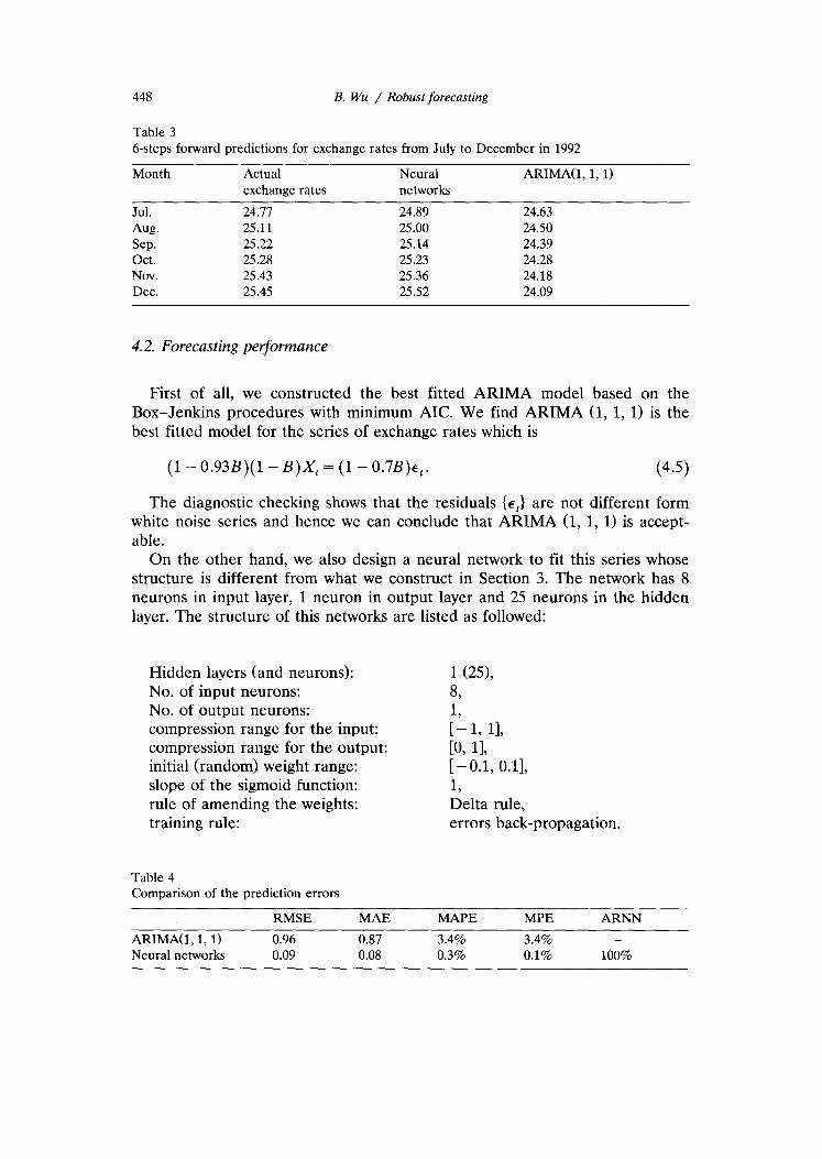
Table 3 6-steps forward predictions for exchange rates from July to December in 1992

Month Actual exchange rates

Neural networks

ARIMA(1, 1, 1)

Jul. 24.11 24.89 24.63 Aug. 25.11 25.00 24.50 Sep. 25.22 25.14 24.39 Ott. 25.28 25.23 24.28 Nov. 25.43 25.36 24.18 Dec. 25.45 25.52 24.09

4.2. Forecasting performante

First of all, we constructed the best fitted ARIMA model based on the Box-Jenkins procedures with minimum AIC. We find ARIMA (1, 1, 1) is the best fitted model for the series of exchange rates which is

(1 - 0.93B)(l- B)X, = (1 - 0.7+,. (4.5)

The diagnostic checking Shows that the residuals {er} are not different form white noise series and hence we tan conclude that ARIMA (1, 1, 1) is acceptable.

On the other hand, we also design a neural network to fit this series whose structure is different from what we construct in Section 3. The network has 8 neurons in input layer, 1 neuron in output layer and 25 neurons in the hidden layer. The structure of this networks are listed as followed:

Hidden layers (and neurons): No. of input neurons: No. of output neurons: compression range for the input: compression range for the output: initial (random) weight range: slope of the sigmoid function: rule of amending the weights: training rule:

Table 4 Comparison of the prediction errors

1 cm 8, $1 11, [O, 1;, [ - 0.1, 0.11, 1, Delta rule, errors back-propagation.

ARIh4A(l, 1, 1) Neural networks

RMSE MAE 0.96 0.87 0.09 0.08

MAPE 3.4% 0.3%

MPE 3.4% 0.1%

ARNN -

100%


Table 5 One-step-ahead predictions for exchange rates from July to December in 1992

Month

Jul. Aug. Sep. Ott. Nov. Dec.

Actual Neural exchange rates networks

24.77 24.89 25.11 24.87 25.22 25.22 25.28 25.28 25.43 25.35 25.45 25.42

ARIMA(1, 1, 1)

24.63 24.68 25.13 25.26 25.31 25.49

The network has trained for about 80 epochs. We compare its 6-steps forward and one-step-ahead predictions results with ARIMA’s in Tables 3 to 6. Figures 5 and 6 show the tendencies of the actual values and predictions by ARIMA(l, 1, 1) and neural networks.

On the other hand, we consider the Performance of forecasting by using of the structure changed model. It is not surprising that the best fitted ARIMA model is ARIMA(1, 1, 01,

(1 - 0.28B)(l -B)X, = E,.

The diagnostic checking Shows that the residuals {et) follow the white noise process and normal. So we accept ARIMA (1, 1,O) as an adequated model. The one-step-ahead forecasting comparisons between ARIMA model and neural networks are exhibited in Table 7 and 8.

From the above forecasting Performance, we conclude that the neural networks perform a robust forecasting. From March 1992 to June 1992, the exchange rates described a type of the decreasing trend. If we make use of the ARIMA(1, 1, 1) model to forecast the forthcoming months, the prediction values tan hardly trace its real tendency. While, the neural networks have traced the real tendency better than ARIMA models in this example, see Figures 5 and 6. Since the Pattern of the exchange rates exhibits certain kind of nonlinear type, neural networks method is suggested for the robust reason.

A special feature should be mentioned is that if we use the second data set in model construction, the Performance of ARIMA model is better than the first data set. We might regard the results as the structure Change which heavily influenced the Parameters estimations. But the neural networks approach which is based on model-free forecasting does not have the same result as ARIMA

Table 6 Comparison of the one-step-ahead prediction errors

ARIMA(1, 1,l) Neural networks

RMSE

0.20 0.16

0.14 0.08

MAPE MPE ARNN

0.6% 0.5% -

0.3% 0.2% 100%


- NETWORKS

-+- EXCH. RATES

26.6

26.2

24.0

24.4

24

, -

, -

l-

L -.

l-

I , , I

/’ <’ ,

/

,’ #’

,’ ._-._ -._--._._.

. .

. . .

..

I I I ,

t , , ,

I , I ,

l , , ,

,*’ ,’

*’ S’

*’ ,’

,’

/

_--.__ --_

._

.-..

1 I 1 ,

. .

-*

-L

.) 1)

163 164 166 166 167 166

Fig. 5’. The tendency of 6-steps forward predictions by ARIMA(1, 1, 1) and neural networks.

models, although its RMSE, MAE, MAPE and MPE are smaller. We should mention again that the larger data set will do a better job than a smaller networks approach and will be applicable for many different kinds of time series analysis if the data set is sufficiently large.


5. Conclusions

This Paper demonstrated the practical applications in forecasting when the underlying models for the observations are uncertain. The advantage of the neural networks technique proposed in this article is that it provides a method-

- NETlJORKS

--t- EXCH. RATES

26.6

26.4

26.2

2I j-

24.t 3-

3-- 24.f

I’

8’

,’ >’

#’ #’

,’

,’ ,’

: 7----- ----- -

I 1 , I

____?.. ._ ..-.-

I I , I I , I I

, I

#’

p _...-.-

__-..

I , , t

-f-- ARItlA<! . . .--.___.-..~

163 164 166 166 167 166 Fig. 6. The tendency of one-step-ahead prediction by ARIMA(1, 1, 1) and neural networks.


Table 7 One-step ahead predictions for exchange rates from July to December 1992

Month

Jul. Aug. Sep. Ott. Nov. Dec.

Actual Neural exchange rates networks

24.77 24.69 25.11 25.16 25.22 25.22 25.28 25.30 25.43 25.33 25.45 25.43

ARIMA(l, 1, 0)

24.73 24.78 25.19 25.25 25.29 25.46

Table 8 Comparison of the onestep ahead prediction errors

RMSE MAE MAPE MPE ARNN

ARIMA(1, 1,l) 0.15 0.1 0.4% -0.4% - Neural networks 0.06 0.05 0.2% -0.1% 67.%

ology for model-free approximation; i.e. the weighted matrix estimation is independent of any models. It has liberated us from the procedures of the model-based selection and the Sample data assumptions. When the nonlinear Systems are still in the early Stage of development, we tan conclude that the neural networks approach suggests a competitive and robust method for the System analysis, forecast and control. The neural network presented is a supe- rior technique in the process of bilinear time series. And the connections between forecasting, data compression, and neurocomputing shown in this Paper seems very interesting in the time series analysis.

In spite of the robust forecast performances for neural networks, there remain some Problems to be solved. For example: (i) How to select the appropriate initial conditions? (ii) How to avoid the Problem of overfitting? (iii) How many input nodes are required for a seasonal time series? (iV> How to find the 95% confidence interval for the forecasts? (v) How to treat the outlier data?

However, in Order to get an appropriate accuracy for arbitraty time series, we hope the neurocomputing will be a worthwhile approach and will stimulate more future empirical work in time series analysis.

References

Box, G.E.P. and G.M. Jenkins, Time series analysis: Forecasting and control, 2nd ed. (Holden-Day, San Francisco 1976).

Brockett, R.W. Volterra series and geometric control theory, Automatica, 12 (1976) 167-176. Chan, W.S. and H. Tong, On test for non-linearity in time series analysis, Intern. J. Forecasting, 5

(1986) 217-28.


Cybento, G., Approximation by superposition of a sigmoidal function, Mathematics of Control, Signals and Systems, 2 (1989) 303-314.

DeGooijer, J.G. and K. Kumar, Some recent developments in nonlinear time series modelling, testing and forecasting. Intern. J. Forecasting, 8 (1992) 135-156.

Engle, R.F., Autoregressive conditional heteroscedasticity with estimates of the variance of U.K. inflation. Econometrica, 50 (1982) 987-1008.

Funahashi, KJ., On the approximate of continuous mappings by neural networks, Neural Networks, 2 (1989) 183-192.

Granger, C.W.J. and A.P. Anderson, An introduction to bilinear time series models (Vandenhoeck and Ruprech Göttingen, 1978).

Granger, C.W.J., Developments in the nonlinear analysis of economic series, Stand. .Z. of Eton., 93 (2) (1991) 263-276.

Grossberg, S., Studies of mind and brain: Neural principles of learning, perception, development, cognition and motor control (Reidel, Boston, MA, 1933).

Guegan, D. and T.D. Pham, Power of the Score test against bilinear time series models, Statistica Sinica, Vol. 2, 1, (1992) 157-169.

Hecht-Nielsen, R., Neurocomputing, ZEEE Spectrum, March (1989) 36-41. Hinich, M., Testing for Gaussianity and linearity of a stationary time series, J. Time Ser. Anal.,

Vol. 3, No. 3 (1982) 169-76. Hornik, K., M. Stinchcombe and H. White, Multilayer feedfoward networks are universal

approximators, Neural Networks, Vol. 2 (19891359-366. Kolen, J.F. and A.K. Goel, Learning in parallel distributed processing networks: Computational

complexity and information content, ZEEE Transattions on Systems, Man, and Cybernetics, 21, 2 (1991) 359-367.

Kosko, B., Neural networks for Signal processing (Prentice Hall, Englewood Cliffs, NJ, 1992). Lapedes, A., and R. Farber, Nonlinear Signal processing using neural networks: prediction and

System modelling, Technical report LA-UR-87-2662 (Los Alamos National Laboratory, Los Alamos, 1987).

Lapedes, A., and R. Farber, How neural nets work, Theoretical Division (Los Alamos National Laboratory Los Alamos, NM 87545, 1988).

Luukkonen, R., P. Saikkonen and T. Terasvirta, Testing linearity against smooth transition autocorrelation models, Biometrica, 75 (1988) 491-500.

McKenzie, E., Some simple models for discrete variate time series, in: K.W. Hipel (Ed.) Time series analysis in water resources, (AM. Water Res. Assoc, 1935) pp. 645-650.

Pesaran, M.H. and S.M. Potter, Nonlinear dynamics and econometrics: An introduction, J. Appl. Econom., 7 (1992) Sl-S7.

Priestley, M.B., State-dependent models: A general approach to nonlinear time series, J. Time Series Anal. 1 (1980) 47-71.

Rumelhart, D.E., G.E. Hinton and R.J. Williams, Learning representations by back-propagation errors, Nature, Vol. 323 (1986) 533-536.

Saikkonen, P. and K. Luukkonen, Lagrange multiplier test for testing non-linearities in time series models, Stand. J. of Statist., 15 (1988) 55-68.

Subba Rao, T. and M.M. Gabr, An introduction to bispectral analysis and bilinear time series models, in: Lecture Notes in Statistics (Springer-Verlag, London, 1984).

Tj0stheim, D. Some doubly stochastic time series models, J. Time Ser. Anal., 7 (1986) 51-72. Tong, H. and K.S. Lim, Threshold autoregression, limit cycles and cyclical data, J. Roy. Statist.

Sec. Ser. B, 42 (1980) 245-292. Tsay, R.S., Detecting and modeling nonlinearity in univariate time series analysis, Statistica Sinica,

Vol. 1, 2 (1991) 431-451. Vogl, T.P., J.K. Mangis, A.K. Rigler, W.T. Zink and D.L. Alkon, Accelerating the convergence of

the back-propagation method, Biological Cybemetics, Vol. 59 (1988) 257-263. Weiss, A.A., ARCH and bilinear time series models: comparison and combination, J. Business&

Eton. Statist., Vol. 4, No. 1 (1986) 59-70.


White, H., Consequences and detection of misspecified nonlinaer regulartion models, J. Amer. Statist. Assoc., Vol. 76 (1981) 419-433.

Wu, B., W. Liou and Y. Chen, Robust forecasting for the stochastic models and chaotic models, J. Chinese Statist. Assoc. Vol. 30, No. 2 (1992) 169-189.

Wu, B. and N. Shih, On the identification Problem for bilinear time series models, .T. Statist. Comput. Simul., Vol. 43 (1992) 129-161.

Appendix A: Tendencies of the simulated bilinear time series

T+, = 20 + 0.2 x, Et + Et+1

iie - . . . .-

88 -

-48 _ _ . . : L . . I * . . . . ., ,

8 iee aee 388 488 6ee 688

q,, = 20 + 0.5 q=, + ct+l


e2e-!_-__’ 1. _j . ..-

326 -- --- -

q,, = 20 + 0.8 x, Et + Et+l


e iee 288 3ee la~..I....I

488 688 688

L, = 20 + 0.2 x, Et.1 + q+1

6e - .

-48 - -. e

1 . . . 1 I

ie8 288 388 488 sec 688

q,, = 20 + 0.5 x, q.1 + E,+1


q,, = 20 + 0.2 x, + 0.2 x, Et + E,+,

iee 288 388 48.8

q,, = 20 + 0.5 x, + 0.5 x, &, + &,+1

688 6ee

458

2780 -

B. Wu / Robust forecasting

1-1 I,, 1, 1, 7, I , I, 1, (

0 10Q 208 300 480 680 6e0

X,,, = 20 + 0.8 X, + 0.8 x, E, + E,+~

68

48

38

28

10

e ~

T

8 iee 288 388 4ee 688 688

X = 1+1 20 + 0.2 x, + 0.2 x, E( - 0.2 x,., Et_, + q+,

e ie0 288 388 488 sec 688

X 1+1 = 20 + 0.5 x, + 0.5 x, Et - 0.5 x,., E,., + Et+1


100 200 380 480 688 688

X <+1 = 20 + 0.8 x, + 0.8 X, E, - 0.8 X,_, q1 + q+,

model-free forecasting for nonlinear time series (with application to exchange rates)

Documents