Model-Driven Data Acquisition in Sensor Networks∗

Amol Deshpande† Carlos Guestrin‡ Samuel R. Madden§ ‡

Joseph M. Hellerstein† ‡ Wei Hong‡

†UC Berkeley ‡ Intel Research Berkeley §MIT{amol,jmh}@cs.berkeley.edu {guestrin,whong}@intel-research.net madden@csail.mit.edu

AbstractDeclarative queries are proving to be an attractive paradigm for in-teracting with networks of wireless sensors. The metaphor that “thesensornet is a database” is problematic, however, because sensorsdo not exhaustively represent the data in the real world. In orderto map the raw sensor readings onto physical reality, amodelofthat reality is required to complement the readings. In this paper,we enrich interactive sensor querying with statistical modeling tech-niques. We demonstrate that such models can help provide answersthat are both more meaningful, and, by introducing approximationswith probabilistic confidences, significantly more efficient to com-pute in both time and energy. Utilizing the combination of a modeland live data acquisition raises the challenging optimization prob-lem of selecting the best sensor readings to acquire, balancing theincrease in the confidence of our answer against the communicationand data acquisition costs in the network. We describe an expo-nential time algorithm for finding the optimal solution to this op-timization problem, and a polynomial-time heuristic for identifyingsolutions that perform well in practice. We evaluate our approach onseveral real-world sensor-network data sets, taking into account thereal measured data and communication quality, demonstrating thatour model-based approach provides a high-fidelity representation ofthe real phenomena and leads to significant performance gains ver-sus traditional data acquisition techniques.

1 IntroductionDatabase technologies are beginning to have a significant im-pact in the emerging area of wireless sensor networks (sen-sornets). The sensornet community has embraced declarativequeries as a key programming paradigm for large sets of sen-sors. This is seen in academia in the calls for papers for lead-ing conferences and workshops in the sensornet area [2, 1],and in a number of prior research publications ([21],[30],[17],etc). In the emerging industrial arena, one of the leading ven-dors (Crossbow) is bundling a query processor with their de-vices, and providing query processor training as part of theircustomer support. The area of sensornet querying representsan unusual opportunity for database researchers to apply theirexpertise in a new area of computer systems.

∗This work was supported by Intel Corporation, and by NSF under thegrant IIS-0205647.

Permission to copy without fee all or part of this material is granted providedthat the copies are not made or distributed for direct commercial advantage,the VLDB copyright notice and the title of the publication and its date appear,and notice is given that copying is by permission of the Very Large Data BaseEndowment. To copy otherwise, or to republish, requires a fee and/or specialpermission from the Endowment.

Proceedings of the 30th VLDB Conference,Toronto, Canada, 2004

Declarative querying has proved powerful in allowing pro-grammers to “task” an entire network of sensor nodes, ratherthan requiring them to worry about programming individ-ual nodes. However, the metaphor that “the sensornet is adatabase” has proven misleading. Databases are typicallytreated as complete, authoritative sources of information; thejob of a database query engine has traditionally been to an-swer a query “correctly” based upon all the available data.Applying this mindset to sensornets results in two problems:

1. Misrepresentations of data: In the sensornet environ-ment, it is impossible to gatherall the relevant data. Thephysically observable world consists of a set of con-tinuous phenomena in both time and space, so the setof relevant data is in principle infinite. Sensing tech-nologies acquiresamplesof physical phenomena at dis-crete points in time and space, but the data acquired bythe sensornet is unlikely to be a random (i.i.d.) sam-ple of physical processes, for a number of reasons (non-uniform placement of sensors in space, faulty sensors,high packet loss rates, etc). So a straightforward inter-pretation of the sensornet readings as a “database” maynot be a reliable representation of the real world.

2. Inefficient approximate queries: Since a sensornetcannot acquire all possible data, any readings from asensornet are “approximate”, in the sense that they onlyrepresent the true state of the world at the discrete in-stants and locations where samples were acquired. How-ever, the leading approaches to query processing in sen-sornets [30, 21] follow a completist’s approach, acquir-ing as much data as possible from the environment at agiven point in time, even whenmost of that data provideslittle benefit in approximate answer quality. We showexamples where query execution cost – in both time andpower consumption – can be orders of magnitude morethan is appropriate for a reasonably reliable answer.

1.1 Our contribution

In this paper, we propose to compensate for both of these defi-ciencies by incorporating statisticalmodelsof real-world pro-cesses into a sensornet query processing architecture. Modelscan help provide more robust interpretations of sensor read-ings: for example, they can account for biases in spatial sam-pling, can help identify sensors that are providing faulty data,and can extrapolate the values of missing sensors or sensorreadings at geographic locations where sensors are no longeroperational. Furthermore, models provide a framework foroptimizing the acquisition of sensor readings: sensors should

be used to acquire data only when the model itself is not suf-ficiently rich to answer the query with acceptable confidence.

Underneath this architectural shift in sensornet querying,we define and address a key optimization problem: given aquery and a model, choose a data acquisition plan for thesensornet to best refine the query answer. This optimizationproblem is complicated by two forms of dependencies: onein the statisticalbenefitsof acquiring a reading, the other inthe systemcostsassociated with wireless sensor systems.

First, any non-trivial statistical model will capture correla-tions among sensors: for example, the temperatures of ge-ographically proximate sensors are likely to be correlated.Given such a model, the benefit of a single sensor reading canbe used to improve estimates of other readings: the tempera-ture at one sensor node is likely to improve the confidence ofmodel-driven estimates for nearby nodes.

The second form of dependency hinges on the connectiv-ity of the wireless sensor network. If a sensor nodefar isnot within radio range of the query source, then one can-not acquire a reading fromfar without forwarding the re-quest/result pair through another nodenear. This presentsnot only a non-uniform cost model for acquiring readings, butone with dependencies: due to multi-hop networking, the ac-quisition cost fornear will be much lower if one has alreadychosen to acquire data fromfar by routing throughnear.

To explore the benefits of the model-based querying ap-proach we propose, we are building a prototype called BBQ1

that uses a specific model based on time-varying multivari-ate Gaussians. We describe how our generic model-based ar-chitecture and querying techniques are specifically applied inBBQ. We also present encouraging results on real-world sen-sornet trace data, demonstrating the advantages that modelsoffer for queries over sensor networks.

2 Overview of approachIn this section, we provide an overview of our basic architec-ture and approach, as well as a summary of BBQ. Our archi-tecture consists of a declarative query processing engine thatuses a probabilistic model to answer questions about the cur-rent state of the sensor network. We denote a model as aprob-ability density function(pdf), p(X1, X2, . . . , Xn), assigninga probability for each possible assignment to the attributesX1, . . . , Xn, where eachXi is an attribute at a particular sen-sor (e.g., temperature on sensing node 5, voltage on sensingnode 12). Typically, there is one such attribute per sensortype per sensing node. This model can also incorporatehid-den variables(i.e., variables that are not directly observable)that indicate, for example, whether a sensor is giving faultyvalues. Such models can be learned from historical data usingstandard algorithms (e.g., [23]).

Users query for information about the values of particu-lar attributes or in certain regions of the network, much asthey would in a traditional SQL database. Unlike databasequeries, however, sensornet queries request real-time infor-mation about the environment, rather than information abouta stored collection of data. The model is used to estimatesensor readings in the current time period; these estimatesform the answer the query. In the process of generating these

1BBQ is short for Barbie-Q: A Tiny-Model Query System

Probabilistic Model and Planner

Observation Plan

Probabilistic Queries Query Results

Query Processor

"SELECT nodeId, temp ± .1°C, conf(.95) WHERE nodeID in {1..8}"

"1, 22.3 97% 2, 25.6 99% 3, 24.4 95% 4, 22.1 100% ..."

"{[voltage,1], [voltage,2], [temp,4]}"

Data"1, voltage = 2.73 2, voltage = 2.65 4, temp = 22.1"

1

2

3

4

5 6

7

8

Sensor Network

202224262830

1 2 3 4

Sensor ID

Cel

sius

User

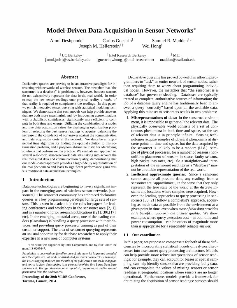
Figure 1:Our architecture for model-based querying in sensor net-works.

estimates, the model may interrogate the sensor network forupdated readings that will help to refine estimates for whichits uncertainty is high. As time passes, the model may alsoupdate its estimates of sensor values, to reflect expected tem-poral changes in the data.

In BBQ, we use a specific model based on time-varyingmultivariate Gaussians; we describe this model below. Weemphasize, however, that our approach is general with re-spect to the model, and that more or less complex modelscan be used instead. New models require no changes to thequery processor and can reuse code that interfaces with andacquires particular readings from the sensor network. Themain difference occurs in the algorithms required to solve theprobabilistic inference tasks described in Section 3. Thesealgorithms have been widely developed for many practicalmodels (e.g., [23]).

Figure 1 illustrates our basic architecture through an ex-ample. Users submit SQL queries to the database, whichare translated into probabilistic computations over the model(Section 3). The queries include error tolerances and tar-get confidence bounds that specify how much uncertainty theuser is willing to tolerate. Such bounds will be intuitive tomany scientific and technical users, as they are the same as theconfidence bounds used for reporting results in most scientificfields (c.f., the graph-representation shown in the upper rightof Figure 1). In this example, the user is interested in esti-mates of the value of sensor readings for nodes numbered 1through 8, within .1 degrees C of the actual temperature read-ing with 95% confidence. Based on the model, the system de-cides that the most efficient way to answer the query with therequested confidence is to read battery voltage from sensors 1and 2 and temperature from sensor 4. Based on knowledge ofthe sensor network topology, it generates anobservation planthat acquires samples in this order, and sends the plan into thenetwork, where the appropriate readings are collected. Thesereadings are used to update the model, which can then be usedto generate query answers with specified confidence intervals.

Notice that the model in this example chooses to observethe voltage at some nodes despite the fact that the user’s query

0 500 1000 1500 2000 2500 3000 350015

20

25

30Reading # vs. Voltage and Temperature

Tem

pera

ture

0 500 1000 1500 2000 2500 3000 35002.6

2.65

2.7

2.75

2.8

2.85

Vol

tage

Reading #

Sensor 1Sensor 25

Sensor 1Sensor 25

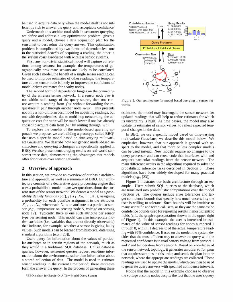
Figure 2:Trace of voltage and temperature readings over a two dayperiod from a single mote-based sensor. Notice the close correlationbetween the two attributes.

was over temperature. This happens for two reasons:

1. Correlations in Value: Temperature and voltage arehighly correlated, as illustrated by Figure 2 which showsthe temperature and voltage readings for two days ofsensor readings from a pair of Berkeley Mica2 Motes [6]that we deployed in the Intel Research Lab in Berkeley,California. Note how voltage tracks temperature, andhow temperature variations across motes, even thoughof noticeably different magnitudes, are very similar. Therelationship between temperature and voltage is due tothe fact that, for many types of batteries, as they heator cool, their voltages vary significantly (by as much as1% per degree). The voltages may also decrease as thesensor nodes consume energy from the batteries, but thetime scale at which that happens is much larger than thetime scale of temperature variations, and so the modelcan use voltage changes to infer temperature changes.

2. Cost Differential: Depending on the specific type oftemperature sensor used, it may be much cheaper tosample the voltage than to read the temperature. Forexample, on sensor boards from Crossbow Corporationfor Berkeley Motes [6], the temperature sensor requiresseveral orders of magnitude more energy to sample assimply reading battery voltage (see Table 1).

One of the important properties of many probabilistic mod-els (including the one used in BBQ) is that they can capturecorrelations between different attributes. We will see how wecan exploit such correlations during optimization to generateefficient query plans in Section 4.

2.1 Confidence intervals and correlation models

The user in Figure 1 could have requested 100% confidenceand no error tolerance, in which case the model would haverequired us to interrogate every sensor. The returned resultcould still include some uncertainty, as the model may nothave readings from particular sensors or locations at somepoints in time (due to sensor or communications failures, orlack of sensor instrumentation at a particular location). Theseconfidence intervals computed from our probabilistic modelprovide considerably more information than traditional sen-sor network systems like TinyDB and Cougar provide in thissetting. With those systems, the user would simply get nodata regarding those missing times and locations.

Conversely, the user could have requested very wide confi-dence bounds, in which case the model may have been able toanswer the query without acquiring any additional data fromthe network. In fact, in our experiments with BBQ on sev-eral real-world data sets, we see a number of cases wherestrong correlations between sensors during certain times ofthe day mean that even queries with relatively tight confi-dence bounds can be answered with a very small number ofsensor observations. In many cases, these tight confidencescan be provideddespite the fact that sensor readings havechanged significantly. This is because known correlations be-tween sensors make it possible to predict these changes: forexample, in Figure 2, it is clear that the temperature on thetwo sensors is correlated given the time of day. During thedaytime (e.g., readings 600-1200 and 2600-3400), sensor 25,which is placed near a window, is consistently hotter than sen-sor 1, which is in the center of our lab. A good model will beable to infer, with high confidence that, during daytime hours,sensor readings on sensor 25 are 1-2 degrees hotter than thoseat sensor 1 without actually observing sensor 25. Again, thisis in contrast to existing sensor network querying systems,where sensors are continuously sampled and readings are al-ways reported whenever small absolute changes happen.

Typically in probabilistic modeling, we pick a class ofmodels, and use learning techniques to pick the best model inthe class. The problem of selecting the right model class hasbeen widely studied (e.g., [23]), but can be difficult in someapplications. Before presenting the specific model class usedin BBQ, we note that, in general, a probabilistic model is onlyas good at prediction as the data used to train it. Thus, it maybe the case that the temperature between sensors 1 and 25would not show the same relationship during a different sea-son of the year, or in a different climate – in fact, one mightexpect that when the outside temperature is very cold, sensor25 will read less than sensor 1 during the day, just as it doesduring the night time. Thus, for models to perform accuratepredictions they must be trained in the kind of environmentwhere they will be used. That does not mean, however, thatwell-trained models cannot deal with changing relationshipsover time; in fact, the model we use in BBQ uses differentcorrelation data depending on time of day. Extending it tohandle seasonal variations, for example is a straightforwardextension of the techniques we use for handling variationsacross hours of the day.

2.2 BBQ

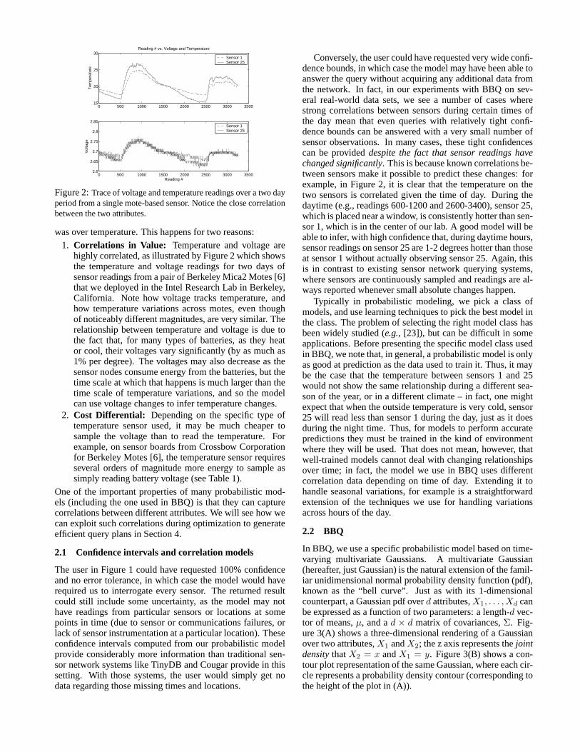
In BBQ, we use a specific probabilistic model based on time-varying multivariate Gaussians. A multivariate Gaussian(hereafter, just Gaussian) is the natural extension of the famil-iar unidimensional normal probability density function (pdf),known as the “bell curve”. Just as with its 1-dimensionalcounterpart, a Gaussian pdf overd attributes,X1, . . . , Xd canbe expressed as a function of two parameters: a length-d vec-tor of means,µ, and ad × d matrix of covariances,Σ. Fig-ure 3(A) shows a three-dimensional rendering of a Gaussianover two attributes,X1 andX2; the z axis represents thejointdensitythatX2 = x andX1 = y. Figure 3(B) shows a con-tour plot representation of the same Gaussian, where each cir-cle represents a probability density contour (corresponding tothe height of the plot in (A)).

Intuitively, µ is the point at the center of this probabilitydistribution, andΣ represents the spread of the distribution.Theith element along the diagonal ofΣ is simply the varianceof Xi. Each off-diagonal elementΣ[i, j], i 6= j representsthe covariance between attributesXi andXj . Covariance isa measure of correlation between a pair of attributes. A highabsolute covariance means that the attributes are strongly cor-related: knowledge of one closely constrains the value of theother. The Gaussians shown in Figure 3(A) and (B) have ahigh covariance betweenX1 andX2. Notice that the contoursare elliptical such that knowledge of one variable constrainsthe value of the other to a narrow probability band.

In BBQ, we use historical data to construct the initial rep-resentation of this pdfp. In the implementation describedin this paper, we obtained such data using TinyDB (a tradi-tional sensor network querying system)2. Once our initialp is constructed, we can answer queries using the model,updating it as new observations are obtained from the sen-sor network, and as time passes. We explain the details ofhow updates are done in Section 3.2, but illustrate it graph-ically with our 2-dimensional Gaussian in Figures 3(B) -3(D). Suppose that we have an initial Gaussian shown in Fig-ure 3(B) and we choose to observe the variableX1; giventhe resulting single value ofX1 = x, the points along theline {(x,X2) | ∀X2 ∈ [−∞,∞]} conveniently form an (un-normalized) one-dimensional Gaussian. After re-normalizingthese points (to make the area under the curve equal 1.0), wecan derive a new pdf representingp(X2 | X1 = x), which isshown in 3(C). Note that the mean ofX2 given the value ofX1 is not the same as the prior mean ofX2 in 3(B). Then, af-ter some time has passed, our belief aboutX1’s value will be“spread out”, and we will again have a Gaussian over twoattributes, although both the mean and variance may haveshifted from their initial values, as shown in Figure 3(D).

2.3 Supported queries

Answering queries probabilistically based on a distribution(e.g., the Gaussian representation described above) is con-ceptually straightforward. Suppose, for example, that a queryasks for anε approximation to the value of a set of attributes,with confidence at least1 − δ. We can use our pdf to com-pute the expected value,µi, of each attribute in the query.These will be our reported values. We can the use the pdfagain to compute the probability thatXi is within ε from themean,P (Xi ∈ [µi − ε, µi + ε]). If all of these probabili-ties meet or exceed user specified confidence threshold, thenthe requested readings can be directly reported as the meansµi. If the model’s confidence is too low, then the we requireadditional readings before answering the query.

Choosing which readings to observe at this point is an opti-mization problem: the goal is to pick the best set of attributesto observe, minimizing the cost of observation required tobring the model’s confidence up to the user specified thresh-old for all of the query predicates. We discuss this optimiza-tion problem in more detail in Section 4.

In Section 3, we show how our query and optimizationengine are used in BBQ to answer a number of SQL queries,

2Though these initial observations do consume some energy up-front, wewill show that the long-run energy savings obtained from using a model willbe much more significant.

5 10 15 20 25 30 35 40

5

10

15

20

25

30

35

40

X2

X 1

Gaussian PDF over X1,X2 where Σ(X1,X2) is Highly Positive

µ=20,20

5 10 15 20 25 30 35 40

5

10

15

20

25

30

35

40Gaussian PDF over X1, X2 after Some Time

X2

X 1

µ=25,25

5 10 15 20 25 30 350

0.02

0.04

0.06

0.08

0.1

0.12

0.14PDF over X2 After Conditioning on X1

Prob

abilit

y(X 2 =

x)

X2

µ=19

010

2030

40

010

2030

400

0.020.040.060.08

0.10.120.14

X1

2D Gaussian PDF With High Covariance (!)

X2

0.02

0.04

0.06

0.08

0.1

0.12

(C)

(A)

(B)

(D)

Figure 3: Example of Gaussians: (a) 3D plot of a 2D Gaussianwith high covariance; (b) the same Gaussian viewed as a contourplot; (c) the resulting Gaussian overX2 after a particular value ofX1 has been observed; finally, (d) shows how, as uncertainty aboutX1 increases from the time we last observed it, we again have a 2DGaussian with a lower variance and shifted mean.

including (i) simple selection queries requesting the value ofone or more sensors, or the value of all sensors in a givengeographic region, (ii) whether or not a predicate over oneor more sensor readings is true, and (iii) grouped aggregatessuch as AVERAGE.

For the purposes of this paper, we focus on multiple one-shot queries over the current state of the network, rather thancontinuous queries. We can provide simple continuous queryfunctionality by issuing a one-shot query at regular time in-tervals. In our experimental section, we compare this ap-proach to existing continuous query systems for sensor net-works (like TinyDB). We also discuss how knowledge of astanding, continuous query could be used to further optimizeour performance in Section 6.

In this paper, there are certain types of queries which wedo not address. For example, BBQ is not designed for out-lier detection – that is, it will not immediately detect when asingle sensor is reading something that is very far from itsexpected value or from the value of neighbors it has beencorrelated with in the past. We suggest ways in which ourapproach can be amended to handle outliers in Section 6.

2.4 Networking model and observation plan format

Our initial implementation of BBQ focuses on static sensornetworks, such as those deployed for building and habitatmonitoring. For this reason, we assume that network topolo-gies change relatively slowly. We capture network topologyinformation when collecting data by including, for each sen-sor, a vector of link quality estimates for neighboring sensornodes. We use this topology information when constructingquery plans by assuming that nodes that were previously con-nected will still be in the near future. When executing a plan,if we observe that a particular link is not available (e.g., be-cause one of the sensors has failed), we update our topologymodel accordingly.We can continue to collect new topologyinformation as we query the network, so that new links willalso become available. This approach will be effective if the

topology is relatively stable; highly dynamic topologies willneed more sophisticated techniques, which is a problem webriefly discuss in Section 6.

In BBQ, observation plans consist of a list of sensor nodesto visit, and, at each of these nodes, a (possibly empty) listof attributes that need to be observed at that node. The possi-bility of visiting a node but observing nothing is included toallow plans to observe portions of the network that are sepa-rated by multiple radio hops. We require that plans begin andend at sensor id 0 (theroot), which we assume to be the nodethat interfaces the query processor to the sensor network.

2.5 Cost model

During plan generation and optimization, we need to be ableto compare the relative costs of executing different plans inthe network. As energy is the primary concern in battery-powered sensornets [15, 26], our goal is to pick plans of min-imum energy cost. The primary contributors to energy costare communication and data acquisition from sensors (CPUoverheads beyond what is required when acquiring and send-ing data are small, as there is no significant processing doneon the nodes in our setting).

Our cost model uses numbers obtained from the datasheets of sensors and the radio used on Mica2 motes witha Crossbow MTS400 [6] environmental sensor board. Forthe purposes of our model, we assume that the sender and re-ceiver are well synchronized, so that a listening sensor turnson its radio just as a sending node begins transmitting3. Oncurrent generation motes, the time required to send a packetis about 27 ms. The ChipCon CC1000 radio on motes usesabout 15 mW of energy in both send and receive modes,meaning that both sender and receiver consume about .4 mJof energy. Table 1 summarizes the energy costs of acquiringreadings from various sensors available for motes. In this pa-per, we primarily focus on temperature readings, though webriefly discuss other attributes as well in Section 5. Assum-ing we are acquiring temperature readings (which cost .5 Jper sample), we compute the cost of a plan that visitss nodesand acquiresa readings to be(.4× 2)× s+.5× a if there areno lost packets. In Section 4.1, we generalize this idea, andconsider lossy communication. Note that this cost treats theentire network as a shared resource in which power needs tobe conserved equivalently on each mote. More sophisticatedcost models that take into account the relative importance ofnodes close to the root could be used, but an exploration ofsuch cost models is not needed to demonstrate the utility ofour approach.

3 Model-based querying

As described above, the central element in our approach isthe use of a probabilistic model to answer queries about theattributes in a sensor network. This section focuses on a fewspecific queries: range predicates, attribute-value estimates,

3In practice, this is done by having the receiver periodically sample theradio, listening for a preamble signal that indicates a sender is about to begintransmission; when this preamble is heard, it begins listening continuously.Though this periodic radio sampling uses some energy, it is small, becausethe sampling duty cycle can be 1% or less (and is an overhead paid by anyapplication that uses the radio).

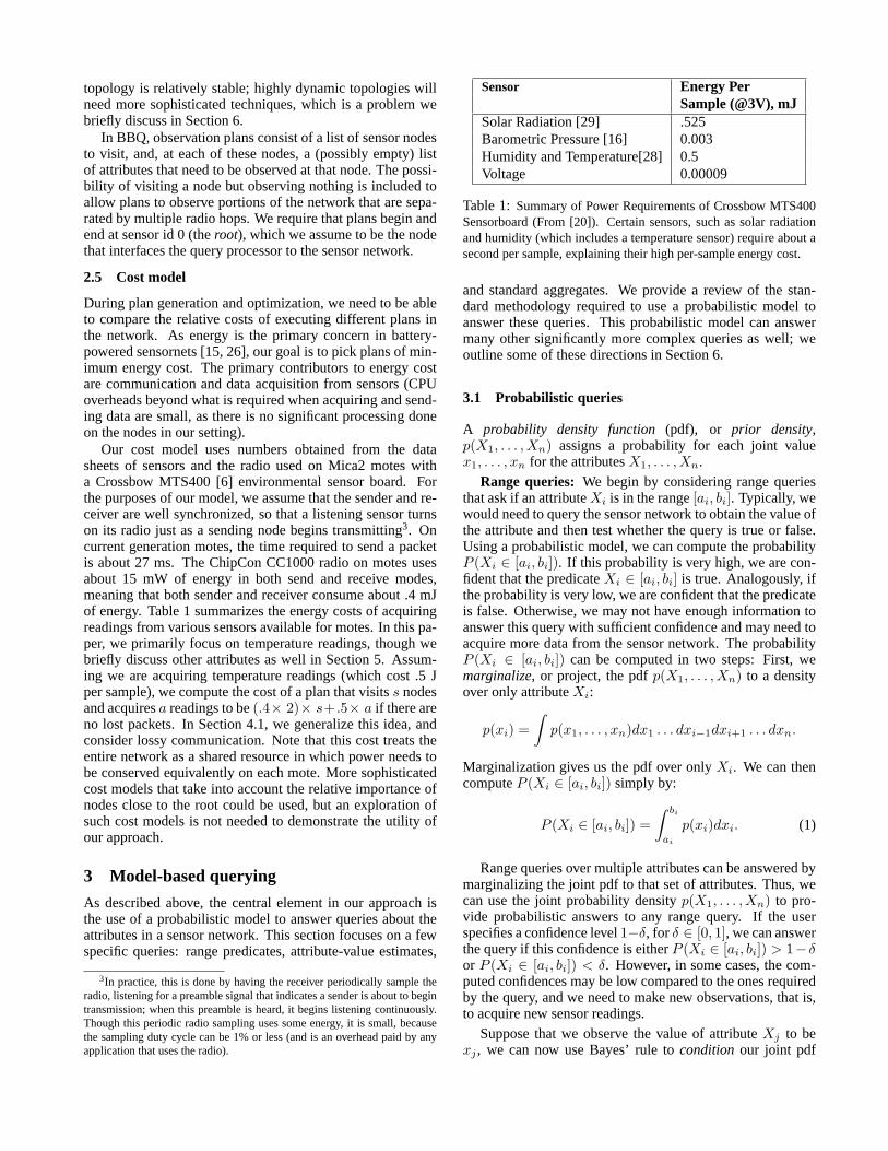
Sensor Energy PerSample (@3V), mJ

Solar Radiation [29] .525Barometric Pressure [16] 0.003Humidity and Temperature[28] 0.5Voltage 0.00009

Table 1: Summary of Power Requirements of Crossbow MTS400Sensorboard (From [20]). Certain sensors, such as solar radiationand humidity (which includes a temperature sensor) require about asecond per sample, explaining their high per-sample energy cost.

and standard aggregates. We provide a review of the stan-dard methodology required to use a probabilistic model toanswer these queries. This probabilistic model can answermany other significantly more complex queries as well; weoutline some of these directions in Section 6.

3.1 Probabilistic queries

A probability density function(pdf), or prior density,p(X1, . . . , Xn) assigns a probability for each joint valuex1, . . . , xn for the attributesX1, . . . , Xn.

Range queries: We begin by considering range queriesthat ask if an attributeXi is in the range[ai, bi]. Typically, wewould need to query the sensor network to obtain the value ofthe attribute and then test whether the query is true or false.Using a probabilistic model, we can compute the probabilityP (Xi ∈ [ai, bi]). If this probability is very high, we are con-fident that the predicateXi ∈ [ai, bi] is true. Analogously, ifthe probability is very low, we are confident that the predicateis false. Otherwise, we may not have enough information toanswer this query with sufficient confidence and may need toacquire more data from the sensor network. The probabilityP (Xi ∈ [ai, bi]) can be computed in two steps: First, wemarginalize, or project, the pdfp(X1, . . . , Xn) to a densityover only attributeXi:

p(xi) =∫

p(x1, . . . , xn)dx1 . . . dxi−1dxi+1 . . . dxn.

Marginalization gives us the pdf over onlyXi. We can thencomputeP (Xi ∈ [ai, bi]) simply by:

P (Xi ∈ [ai, bi]) =∫ bi

ai

p(xi)dxi. (1)

Range queries over multiple attributes can be answered bymarginalizing the joint pdf to that set of attributes. Thus, wecan use the joint probability densityp(X1, . . . , Xn) to pro-vide probabilistic answers to any range query. If the userspecifies a confidence level1−δ, for δ ∈ [0, 1], we can answerthe query if this confidence is eitherP (Xi ∈ [ai, bi]) > 1− δor P (Xi ∈ [ai, bi]) < δ. However, in some cases, the com-puted confidences may be low compared to the ones requiredby the query, and we need to make new observations, that is,to acquire new sensor readings.

Suppose that we observe the value of attributeXj to bexj , we can now use Bayes’ rule tocondition our joint pdf

p(X1, . . . , Xn) on this value4, obtaining:

p(X1, . . . , Xj−1, Xj+1, . . . , Xn | xj) =p(X1, . . . , Xj−1, xj , Xj+1, . . . , Xn)

p(xj).

The conditional probability density functionp(X1, . . . , Xj−1, Xj+1, . . . , Xn | xj), also referred as theposterior densitygiven the observationxj , will usually leadto a more confident estimate of the probability ranges. Usingmarginalization, we can computeP (Xi ∈ [ai, bi] | xj),which is often more certain than the prior probabilityP (Xi ∈ [ai, bi]). In general, we will make a set of observa-tionso, and, after conditioning on these observations, obtainp(X | o), the posterior probability of our set of attributesXgiveno.

Example 3.1 In BBQ, the pdf is represented by a multivari-ate Gaussian with mean vectorµ and covariance matrixΣ.In Gaussians, marginalization is very simple. If we want tomarginalize the pdf to a subsetY of the attributes, we sim-ply select the entries inµ and Σ corresponding to these at-tributes, and drop the other entries obtaining a lower dimen-sional mean vectorµY and covariance matrixΣYY. For aGaussian, there is no closed-form solution for Equation (1).However, this integration problem is very well understood,called theerror function(erf), with many well-known, simpleapproximations.

Interestingly, if we condition a Gaussian on the value ofsome attributes, the resulting pdf is also a Gaussian. Themean and covariance matrix of this new Gaussian can becomputed by simple matrix operations. Suppose that we ob-serve valueo for attributesO, the meanµY|o and covariancematrixΣY|o of the pdfp(Y | o) over the remaining attributesare given by:

µY|o = µY + ΣYOΣ−1OO(o− µO),

ΣY|o = ΣYY − ΣYOΣ−1OOΣOY,

(2)

whereΣYO denotes the matrix formed by selecting the rowsY and the columnsO from the original covariance matrixΣ. Note that the posterior covariance matrixΣY|o does notdepend on the actual observed valueo. We thus denote thismatrix byΣY|O. In BBQ, by using Gaussians, we can thuscompute all of the operations required to answer our queriesby performing only basic matrix operations.2

Value queries: In addition to range queries, a probabilitydensity function can, of course, be used to answer many otherquery types. For example, if the user is interested in the valueof a particular attributeXi, we can answer this query by usingthe posterior pdf to compute the meanx̄i value ofXi, giventhe observationso:

x̄i =∫

xi p(xi | o)dxi.

4The expressionp(x|y) is read “the probability ofx giveny”, and repre-sents the pdf of variablex given a particular value ofy. Bayes’ rule allowsconditional probabilities to be computed in scenarios where we only have

data on the inverse conditional probability:p(x|y) =p(y|x)p(x)

p(y).

We can additionally provide confidence intervals on this esti-mate of the value of the attribute: for a given error boundε >0, the confidence is simply given byP (Xi ∈ [x̄i−ε, x̄i +ε] |o), which can be computed as in the range queries in Equa-tion (1). If this confidence is greater than the user specifiedvalue1 − δ, then we can provide a probably approximatelycorrect value for the attribute, without observing it.

AVERAGE aggregates: Average queries can be an-swered in a similar fashion, by defining an appropriate pdf.Suppose that we are interested in the average value of a setof attributesA. For example, if we are interested in the av-erage temperature in a spatial region, we can defineA to bethe set of sensors in this region. We can now define a randomvariableY to represent this average byY = (

∑i∈A Xi)/|A|.

The pdf forY is simply given by appropriate marginalizationof the joint pdf over the attributes inA:

p(Y = y | o) =∫p(x1, . . . , xn | o) 1

[(∑i∈A

xi/|A|

)= y

]dx1 . . . dxn,

where1[·] is the indicator function.5 Oncep(Y = y | o) isdefined, we can answer an average query by simply defininga value query for the new random variableY as above. Wecan also compute probabilistic answers to more complex ag-gregation queries. For example, if the user wants the averagevalue of the attributes inA that have value greater thant, wecan define a random variableZ:

Z =∑

i∈A Xi1(Xi > c)∑i∈A 1(Xi > c)

,

where00 is defined to be0. The pdf ofZ is given by:

p(Z = z | o) =∫p(x1, . . . , xn | o) 1

[(∑i∈A,xi>c xi∑i∈A,xi>c 1

)= y

]dx1 . . . dxn.

In general, this inference problem,i.e., computing these in-tegrals, does not have a closed-form solution, and numericalintegration techniques may be required.

Example 3.2 BBQ focuses on Gaussians. In this case, eachposterior mean̄xi can be obtained directly from our meanvector by using the conditioning rule described in Exam-ple 3.1. Interestingly, the sum of Gaussian random variablesis also Gaussian. Thus, if we define an AVERAGE queryY = (

∑i∈A Xi)/|A|, then the pdf forY is a Gaussian. All

we need now is the variance ofY , which can be computed inclosed-form from those of eachXi by:

E[(Y − µY )2] = E[(∑

i∈A Xi − µi)2/|A|2],= 1

|A|2(∑

i∈A E[(Xi − µi)2]+2∑

i∈A∑

j∈A,j 6=i

E[(Xi − µi)(Xj − µj)]) .

Thus, the variance ofY is given by a weighted sum of the

5The indicator function translates a Boolean predicate into the arithmeticvalue 1 (if the predicate is true) and 0 (if false).

variances of eachXi, plus the covariances betweenXi andXj , all of which can be directly read off the covariance ma-trix Σ. Therefore, we can answer an AVERAGE query over asubset of the attributesA in closed-form, using the same pro-cedure as value queries. For the more general queries thatdepend on the actual value of the attributes, even with Gaus-sians, we require a numerical integration procedure.2

3.2 Dynamic models

Thus far, we have focused on a single static probability den-sity function over the attributes. This distribution representsspatialcorrelation in our sensor network deployment. How-ever, many real-world systems include attributes that evolveover time. In our deployment, the temperatures have bothtemporal and spatial correlations. Thus, the temperature val-ues observed earlier in time should help us estimate the tem-perature later in time. Adynamic probabilistic modelcanrepresent such temporal correlations.

In particular, for each (discrete) time indext, we shouldestimate a pdfp(Xt

1, . . . , Xtn | o1...t) that assigns a prob-

ability for each joint assignment to the attributes at timet, given o1...t, all observations made up to timet. A dy-namic model describes the evolution of this system over time,telling us how to computep(Xt+1

1 , . . . , Xt+1n | o1...t) from

p(Xt1, . . . , X

tn | o1...t). Thus, we can use all measurements

made up to timet to improve our estimate of the pdf at timet + 1.

For simplicity, we restrict our presentation toMarkovianmodels, where given the value ofall attributes at timet, thevalue of the attributes at timet + 1 are independent of thosefor any time earlier thant. This assumption leads to a verysimple, yet often effective, model for representing a stochas-tic dynamical system. Here, the dynamics are summarized bya conditional density called thetransition model:

p(Xt+11 , . . . , Xt+1

n | Xt1, . . . , X

tn).

Using this transition model, we can computep(Xt+1

1 , . . . , Xt+1n | o1...t) using a simple marginaliza-

tion operation:

p(xt+11 , . . . , xt+1

n | o1...t) =Zp(xt+1

1 , . . . , xt+1n | xt

1, . . . , xtn)p(xt

1, . . . , xtn | o1...t)dxt

1 . . . dxtn.

This formula assumes that the transition modelp(Xt+1 | Xt)is the same for all timest. In our deployment, for example,in the mornings the temperatures tend to increase, while atnight they tend to decrease. This suggests that the transitionmodel should be different at different times of the day. In ourexperimental results in Section 5, we address this problem bysimply learning a different transition modelpi(Xt+1 | Xt)for each houri of the day. At a particular timet, we simplyuse the transition modelmod(t, 24). This idea can, of course,be generalized to other cyclic variations.

Once we have obtainedp(Xt+11 , . . . , Xt+1

n | o1...t), theprior pdf for timet + 1, we can again incorporate the mea-surementsot+1 made at timet + 1, as in Section 3.1, obtain-ing p(Xt+1

1 , . . . , Xt+1n | o1...t+1), the posterior distribution

at timet + 1 given all measurements made up to timet + 1.

This process is then repeated for timet + 2, and so on.The pdf for the initial timet = 0, p(X0

1 , . . . , X0n), is ini-

tialized with the prior distribution for attributesX1, . . . , Xn.This process of pushing our estimate for the density at timet through the transition model and then conditioning on themeasurements at timet + 1 is often calledfiltering. In con-trast to the static model described in the previous section, fil-tering allows us to condition our estimate on the completehistory of observations, which, as we will see in Section 5,can significantly reduce the number of observations requiredfor obtaining confident approximate answers to our queries.

Example 3.3 In BBQ, we focus on Gaussian distributions;for these distributions the filtering process is called aKalman filter. The transition modelp(Xt+1

1 , . . . , Xt+1n |

Xt1, . . . , X

tn) can be learned from data with two simple steps:

First, we learn a mean and covariance matrix for the jointdensityp(Xt+1

1 , . . . , Xt+1n , Xt

1, . . . , Xtn). That is, we form

tuples⟨Xt+1

1 , . . . , Xt+1n , Xt

1, . . . , Xtn

⟩for our attributes at

every consecutive timest and t + 1, and use these tuples tocompute the joint mean vector and covariance matrix. Then,we use the conditioning rule described in Example 3.1 tocompute the transition model:

p(Xt+1 | Xt) =p(Xt+1,Xt)

p(Xt).

Once we have obtained this transition model, we can answerour queries in a similar fashion as described in Examples 3.1and 3.2. 2

4 Choosing an observation plan

In the previous section, we showed that our pdfs can be condi-tioned on the valueo of the set of observed attributes to obtaina more confident answer to our query. Of course, the choiceof attributes that we observe will crucially affect the result-ing posterior density. In this section, we focus on selectingthe attributes that are expected to increase the confidences inthe answer to our particular query at minimal cost. We firstformalize the notion of cost of observing a particular set ofattributes. Then, we describe the expected improvement inour answer from observing this set. Finally, we discuss theproblem of optimizing the choice of attributes.

4.1 Cost of observations

Let us denote a set of observations byO ⊆ {1, . . . , n}. Theexpected costC(O) of observing attributesO is divided addi-tively into two parts: the data acquisition costCa(O), repre-senting the cost of sensing these attributes, and the expecteddata transmission costCt(O), measuring the communicationcost required to download this data.

The acquisition costCa(O) is deterministically given bythe sum of the energy required to observe the attributesO, asdiscussed in Section 2.5:

Ca(O) =∑i∈O

Ca(i),

whereCa(i) is the cost of observing attributeXi.

The definition of the transmission costCt(O) is somewhattrickier, as it depends on the particular data collection mech-anism used to collect these observations from the network,and on the network topology. Furthermore, if the topology isunknown or changes over time, or if the communication linksbetween nodes are unreliable, as in most sensor networks, thiscost function becomes stochastic. For simplicity, we focus onnetworks with known topologies, but with unreliable com-munication. We address this reliability issue by introducingacknowledgment messages and retransmissions.

More specifically, we define our network graph by a set ofedgesE , where each edgeeij is associated two link qual-ity estimates,pij and pji, indicating the probability that apacket fromi will reach j and vice versa. With the sim-plifying assumption that these probabilities are independent,the expected number of transmission and acknowledgmentmessages required to guarantee a successful transmission be-tweeni andj is 1

pijpji. We can now use these simple values

to estimate the expected transmission cost.There are many possible mechanisms for traversing the

network and collecting this data. We focus on simply choos-ing a single path through the network that visits all sensorsthat observe attributes inO and returns to the base station.Clearly, choosing the best such path is an instance of thetraveling salesman problem, where the graph is given bythe edgesE with weights 1

pijpji. Although this problem is

NP-complete, we can use well-known heuristics, such as k-OPT [19], that are known to perform very well in practice.We thus defineCt(O) to be the expected cost of this (subop-timal) path, and our expected total cost for observingO cannow be obtained byC(O) = Ca(O) + Ct(O).

4.2 Improvement in confidence

Observing attributesO should improve the confidence of ourposterior density. That is, after observing these attributes, weshould be able to answer our query with more certainty6. Fora particular valueo of our observationsO, we can computethe posterior densityp(X1, . . . , Xn | o) and estimate ourconfidence as described in Section 3.1.

More specifically, suppose that we have a range queryXi ∈ [ai, bi], we can compute the benefitRi(o) of observ-ing the specific valueo by:

Ri(o) = max [P (Xi ∈ [ai, bi] | o), 1− P (Xi ∈ [ai, bi] | o)] ,

that is, for a range query,Ri(o) simply measures our confi-dence after observingo. For value and average queries, wedefine the benefit byRi(o) = P (Xi ∈ [x̄i − ε, x̄i + ε] | o),wherex̄i in this formula is the posterior mean ofXi given theobservationso.

However, the specific valueo of the attributesO is notknowna priori. We must thus compute theexpected benefitRi(O):

Ri(O) =∫

p(o)Ri(o)do. (3)

This integral may be difficult to compute in closed-form, andwe may need to estimateRi(O) using numerical integration.

6This is not true in all cases; for range predicates, the confidence in theanswer maydecreaseafter an observation, depending on the observed value.

Example 4.1 The descriptions in Examples 3.1-3.3 describehow the benefitsRi(o) can be computed for a particular ob-served valueo in the Gaussian models used in BBQ. For gen-eral range queries, even with Gaussians, we need to use nu-merical integration techniques to estimate the expected re-wardRi(O) in Equation (3).

However, for value and AVERAGE queries we can com-pute this expression in closed-form, by exploiting the fact de-scribed in Example 3.1 that the posterior covarianceΣY|Odoes not depend on the observed valueo. Note that for thesequeries, we are computing the probability that the true valuedeviates by more thanε from the posterior mean value. Thisprobability is equal to the probability that a zero mean Gaus-sian, with covarianceΣY|O, deviates by more thanε from0. This probability can be computed using the error function(erf) and the covariance matrixΣY|O. Thus, for value andAVERAGE queriesRi(O) = Ri(o),∀o, allowing us to com-pute Equation (3) in closed-form.2

More generally, we may have range or value queries overmultiple attributes. Semantically, we define this type of queryas trying to achieve a particular marginal confidence overeach attribute. We must thus decide how to trade off con-fidences between different attributes. For a query over at-tributesQ ⊆ {1, . . . , n}, we can, for instance, define the to-tal benefitR(o) of observing valueo as either the minimumbenefit over all attributes,R(o) = mini∈Q Ri(o), or the av-erage,R(o) = 1

|Q|∑

i∈Q Ri(o). In this paper, we focus onminimizing the total number of mistakes made by the queryprocessor, and use the average benefit to decide when to stopobserving new attributes.

4.3 Optimization

In the previous sections, we defined the expected benefitR(O) and costC(O) of observing attributesO. Of course,different sets of observed attributes will lead to different ben-efit and cost levels. Our user will define a desired confidencelevel1− δ. We would like to pick the set of attributesO thatmeet this confidence at a minimum cost:

minimizeO⊆{1,...,n} C(O),such that R(O) ≥ 1− δ.

This general optimization problem is known to be NP-hard.Thus, efficient and exact optimization algorithms are unlikelyto exist (unless P=NP).

We have developed two algorithms for solving this opti-mization problem. The first algorithm exhaustively searchesover the possible subsets of possible observations,O ⊆{1, . . . , n}. This algorithm can thus find the optimal subsetof attributes to observe, but has an exponential running time.

The second algorithm uses a greedy incremental heuris-tic. We initialize the search with an empty set of attributes,O = ∅. At each iteration, for each attributeXi that is not inour set (i 6∈ O), we compute the new expect benefitR(O∪ i)and costC(O ∪ i). If some set of attributesG reach the de-sired confidence, (i.e., for j ∈ G, R(O ∪ j) ≥ 1 − δ), then,among the attributes inG, we pick the one with lowest totalcostC(O∪j), and terminate the search returningO∪j. Oth-erwise, ifG = ∅, we have not reached our desired confidence,and we simply add the attribute with the highest benefit over

cost ratio to our set of attributes:

O = O ∪(

arg maxj 6∈O

R(O ∪ j)C(O ∪ j)

).

This process is then repeated until the desired confidence isreached.

5 Experimental resultsIn this section, we measure the performance of BBQ on sev-eral real world data sets. Our goal is to demonstrate that BBQprovides the ability to efficiently execute approximate querieswith user-specifiable confidences.

5.1 Data sets

Our results are based on running experiments over two real-world data sets that we have collected during the past fewmonths using TinyDB. The first data set,garden, is a onemonth trace of 83,000 readings from 11 sensors in a singleredwood tree at the UC Botanical Garden in Berkeley. In thiscase, sensors were placed at 4 different altitudes in the tree,where they collected collected light, humidity, temperature,and voltage readings once every 5 minutes. We split this dataset into non-overlapping training and test data sets (with 2/3used for training), and build the model on the training data.

The second data set,lab, is a trace of readings from 54 sen-sors in the Intel Research, Berkeley lab. These sensors col-lected light, humidity, temperature and voltage readings, aswell as network connectivity information that makes it possi-ble to reconstruct the network topology. Currently, the dataconsists of 8 days of readings; we use the first 6 days fortraining, and the last 2 for generating test traces.

5.2 Query workload

We report results for two sets of query workloads:Value Queries: The main type of queries that we antici-

pate users would run on a such a system are queries askingto report the sensor readings at all the sensors, within a spec-ified error boundε with a specified confidenceδ, indicatingthat no more than a fraction1−δ of the readings should devi-ate from their true value byε. As an example, a typical querymay ask for temperatures at all the sensors within 0.5 degreeswith 95% confidence.

Predicate Queries:The second set of queries that we useare selection queries over the sensor readings where the userasks for all sensors that satisfy a certain predicate, and onceagain specifies a desired confidenceδ.

We also looked ataverage queriesasking for averagesover the sensor readings. Due to space constraints, we donot present results for these queries.

5.3 Comparison systems

We compare the effectiveness of BBQ against two simplestrategies for answering such queries :

TinyDB-style Querying: In this model, the query is dis-seminated into the sensor network using an overlay tree struc-ture [22], and at each mote, the sensor reading is observed.The results are reported back to the base station using thesame tree, and are combined along the way back to minimizecommunication cost.

Approximate-Caching: The base-station maintains aview of the sensor readings at all motes that is guaranteedto be within a certain interval of the actual sensor readingsby requiring the motes to report a sensor reading to the base-station if the value of the sensor falls outside this interval.Note that, though this model saves communication cost bynot reporting readings if they do not change much, it does notsave acquisition costs as the motes are required to observe thesensor values at every time step. This approach is inspired bywork by Olstonet al. [24].

5.4 Methodology

BBQ is used to build a model of the training data. This modelincludes a transition model for each hour of the day, based onKalman filters described in Example 3.3 above. We gener-ate traces from the test data by taking one reading randomlyfrom each hour. We issue one query against the model perhour. The model computes thea priori probabilities for eachpredicate (orε bound) being satisfied, and chooses one ormore additional sensor readings to observe if the confidencebounds are not met. After executing the generated observa-tion plan over the network (at some cost), BBQ updates themodel with the observed values from the test data and com-pares predicted values for non-observed readings to the testdata from that hour.

To measure the accuracy of our prediction with valuequeries, we compute the average number of mistakes (perhour) that BBQ made,i.e., how many of the reported val-ues are further away from the actual values than the specifiederror bound. To measure the accuracy for predicate queries,we compute the number of predicates whose truth value wasincorrectly approximated.

For TinyDB, all queries are answered “correctly” (as weare not modeling loss). Similarly, for approximate caching, avalue from the test data is reported when it deviates by morethanε from the last reported value from that sensor, and assuch, this approach does not make mistakes either

We compute a cost for each observation plan as describedabove; this includes both the attribute acquisition cost andthe communications cost. For most of our experiments, wemeasure the accuracy of our model at predicting temperature.

5.5 Garden dataset: Value-based queries

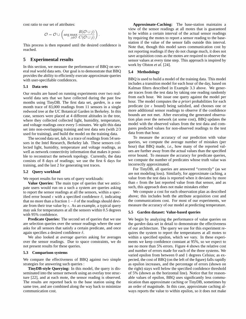
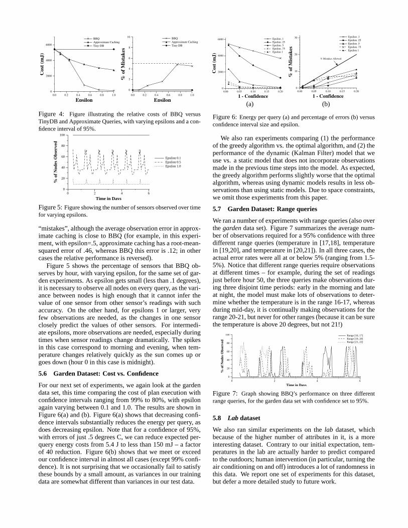
We begin by analyzing the performance of value queries onthegardendata set in detail to demonstrate the effectivenessof our architecture. The query we use for this experiment re-quires the system to report the temperatures at all motes towithin a specified epsilon, which we vary. In these experi-ments we keep confidence constant at 95%, so we expect tosee no more than 5% errors. Figure 4 shows the relative costand number of errors made for each of the three systems. Wevaried epsilon from between 0 and 1 degrees Celsius; as ex-pected, the cost of BBQ (on the left of the figure) falls rapidlyas epsilon increases, and the percentage of errors (shown onthe right) stays well below the specified confidence thresholdof 5% (shown as the horizontal line). Notice that for reason-able values of epsilon, BBQ uses significantly less commu-nication than approximate caching or TinyDB, sometimes byan order of magnitude. In this case, approximate caching al-ways reports the value to within epsilon, so it does not make

0.0 0.2 0.4 0.6 0.8 1.0

Epsilon

0

2000

4000

6000C

ost (

mJ)

BBQApproximate CachingTiny-DB

0.0 0.2 0.4 0.6 0.8 1.0

Epsilon

0

2

4

6

8

10

% o

f Mis

take

s

BBQApproximate CachingTiny-DB

Figure 4: Figure illustrating the relative costs of BBQ versusTinyDB and Approximate Queries, with varying epsilons and a con-fidence interval of 95%.

0 2 4 6

Time in Days

0

20

40

60

80

100

% o

f N

odes

Obs

erve

d

Epsilon 0.1Epsilon 0.5Epsilon 1.0

Figure 5:Figure showing the number of sensors observed over timefor varying epsilons.

“mistakes”, although the average observation error in approx-imate caching is close to BBQ (for example, in this experi-ment, with epsilon=.5, approximate caching has a root-mean-squared error of .46, whereas BBQ this error is .12; in othercases the relative performance is reversed).

Figure 5 shows the percentage of sensors that BBQ ob-serves by hour, with varying epsilon, for the same set of gar-den experiments. As epsilon gets small (less than .1 degrees),it is necessary to observe all nodes on every query, as the vari-ance between nodes is high enough that it cannot infer thevalue of one sensor from other sensor’s readings with suchaccuracy. On the other hand, for epsilons 1 or larger, veryfew observations are needed, as the changes in one sensorclosely predict the values of other sensors. For intermedi-ate epsilons, more observations are needed, especially duringtimes when sensor readings change dramatically. The spikesin this case correspond to morning and evening, when tem-perature changes relatively quickly as the sun comes up orgoes down (hour 0 in this case is midnight).

5.6 Garden Dataset: Cost vs. Confidence

For our next set of experiments, we again look at the gardendata set, this time comparing the cost of plan execution withconfidence intervals ranging from 99% to 80%, with epsilonagain varying between 0.1 and 1.0. The results are shown inFigure 6(a) and (b). Figure 6(a) shows that decreasing confi-dence intervals substantially reduces the energy per query, asdoes decreasing epsilon. Note that for a confidence of 95%,with errors of just .5 degrees C, we can reduce expected per-query energy costs from 5.4 J to less than 150 mJ – a factorof 40 reduction. Figure 6(b) shows that we meet or exceedour confidence interval in almost all cases (except 99% confi-dence). It is not surprising that we occasionally fail to satisfythese bounds by a small amount, as variances in our trainingdata are somewhat different than variances in our test data.

0.00 0.05 0.10 0.15 0.20

1 - Confidence

0

2000

4000

6000

Cos

t (m

J)

Epsilon .1Epsilon .25Epsilon .5Epsilon .75Epsilon 1

(a)

0.00 0.05 0.10 0.15 0.20

1 - Confidence

0

10

20

30

% o

f Mis

take

s

Epsilon .1Epsilon .25Epsilon .5Epsilon .75Epsilon 1

% Mistakes Allowed

(b)

Figure 6:Energy per query (a) and percentage of errors (b) versusconfidence interval size and epsilon.

We also ran experiments comparing (1) the performanceof the greedy algorithm vs. the optimal algorithm, and (2) theperformance of the dynamic (Kalman Filter) model that weuse vs. a static model that does not incorporate observationsmade in the previous time steps into the model. As expected,the greedy algorithm performs slightly worse that the optimalalgorithm, whereas using dynamic models results in less ob-servations than using static models. Due to space constraints,we omit those experiments from this paper.

5.7 Garden Dataset: Range queries

We ran a number of experiments with range queries (also overthegardendata set). Figure 7 summarizes the average num-ber of observations required for a 95% confidence with threedifferent range queries (temperature in [17,18], temperaturein [19,20], and temperature in [20,21]). In all three cases, theactual error rates were all at or below 5% (ranging from 1.5-5%). Notice that different range queries require observationsat different times – for example, during the set of readingsjust before hour 50, the three queries make observations dur-ing three disjoint time periods: early in the morning and lateat night, the model must make lots of observations to deter-mine whether the temperature is in the range 16-17, whereasduring mid-day, it is continually making observations for therange 20-21, but never for other ranges (because it can be surethe temperature is above 20 degrees, but not 21!)

0 2 4 6

Time in Days

0

20

40

60

80

100

% o

f N

odes

Obs

erve

d

Range [16, 17]Range [19, 20]Range [21, 22]

Figure 7: Graph showing BBQ’s performance on three differentrange queries, for the garden data set with confidence set to 95%.

5.8 Lab dataset

We also ran similar experiments on thelab dataset, whichbecause of the higher number of attributes in it, is a moreinteresting dataset. Contrary to our initial expectation, tem-peratures in the lab are actually harder to predict comparedto the outdoors; human intervention (in particular, turning theair conditioning on and off) introduces a lot of randomness inthis data. We report one set of experiments for this dataset,but defer a more detailed study to future work.

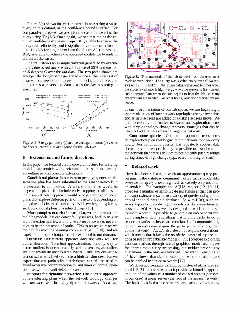
Figure 8(a) shows the cost incurred in answering a valuequery on this dataset, as the confidence bound is varied. Forcomparative purposes, we also plot the cost of answering thequery using TinyDB. Once again, we see that the as the re-quired confidence in answer drops, BBQ is able to answer thequery more efficiently, and is significantly more cost-efficientthan TinyDB for larger error bounds. Figure 8(b) shows thatBBQ was able to achieve the specified confidence bounds inalmost all the cases.

Figure 9 shows an example traversal generated by execut-ing a value based query with confidence of 99% and epsilonof .5 degrees C over thelab data. The two paths shown areamongst the longer paths generated – one is the initial set ofobservations needed to improve the model’s confidence, andthe other is a traversal at 8am just as the day is starting towarm up.

0.00 0.02 0.04 0.06 0.08 0.10

1 - Confidence

0

5000

10000

15000

20000

Cos

t (m

J)

Epsilon 0.25Epsilon 0.5

0.00 0.02 0.04 0.06 0.08 0.10

1 - Confidence

0

5000

10000

15000

20000

Cos

t (m

J)

Epsilon 0.75 Epsilon 1.0

TinyDB

(a)

0.00 0.02 0.04 0.06 0.08 0.10

1 - Confidence

0

5

10

% o

f Mis

take

s

Epsilon 0.25Epsilon 0.5

0.00 0.02 0.04 0.06 0.08 0.100

5

10

Epsilon 0.75Epsilon 1.0

% Mistakes Allowed

(b)

Figure 8:Energy per query (a) and percentage of errors (b) versusconfidence interval size and epsilon for the Lab Data.

6 Extensions and future directions

In this paper, we focused on the core architecture for unifyingprobabilistic models with declarative queries. In this sectionwe outline several possible extensions.

Conditional plans: In our current prototype, once an ob-servation plan has been submitted to the sensor network, itis executed to completion. A simple alternative would beto generate plans that include early stopping conditions; amore sophisticated approach would be to generate conditionalplans that explore different parts of the network depending onthe values of observed attributes. We have begun exploringsuch conditional plans in a related project [8].

More complex models:In particular, we are interested inbuilding models that can detect faulty sensors, both to answerfault detection queries, and to give correct answers to generalqueries in the presence of faults. This is an active researchtopic in the machine learning community (e.g., [18]), and weexpect that these techniques can be extended to our domain.

Outliers: Our current approach does not work well foroutlier detection. To a first approximation, the only way todetect outliers is to continuously sample sensors, as outliersare fundamentally uncorrelated events. Thus, any outlier de-tection scheme is likely to have a high sensing cost, but weexpect that our probabilistic techniques can still be used toavoid excessive communication during times of normal oper-ation, as with the fault detection case.

Support for dynamic networks: Our current approachof re-evaluating plans when the network topology changeswill not work well in highly dynamic networks. As a part

SERVER

LAB

KITCHEN

COPYELEC

PHONEQUIET

STORAGE

CONFERENCE

OFFICEOFFICE50

51

52 53

54

46

48

49

47

43

45

44

42 41

3739

38 36

33

3

6

10

11

12

13 14

1516

17

19

2021

22

242526283032

31

2729

23

18

9

5

8

7

4

34

1

2

3540

0

7-8am Traversal

InitialTraversal

Figure 9: Two traversals of the lab network. An observation ismade at every circle. The query was a value-query over all 54 sen-sors withε = .1 andδ = .99. These paths correspond to times whenthe model’s variance is high – e.g., when the system is first started,and at around 8am when the sun begins to heat the lab, so manyobservations are needed. For other hours, very few observations areneeded.

of our instrumentation of our lab space, we are beginning asystematic study of how network topologies change over timeand as new sensors are added or existing sensors move. Weplan to use this information to extend our exploration planswith simple topology change recovery strategies that can beused to find alternate routes through the network.

Continuous queries: Our current approach re-executesan exploration plan that begins at the network root on everyquery. For continuous queries that repeatedly request dataabout the same sensors, it may be possible to install code inthe network that causes devices to periodically push readingsduring times of high change (e.g., every morning at 8 am).

7 Related workThere has been substantial work on approximate query pro-cessing in the database community, often using model-likesynopsesfor query answering much as we rely on probabilis-tic models. For example, the AQUA project [12, 10, 11]proposes a number of sampling-based synopses that can pro-vide approximate answers to a variety of queries using a frac-tion of the total data in a database. As with BBQ, such an-swers typically include tight bounds on the correctness ofanswers. AQUA, however, is designed to work in an envi-ronment where it is possible to generate an independent ran-dom sample of data (something that is quite tricky to do insensor networks, as losses are correlated and communicatingrandom samples may require the participation of a large partof the network). AQUA also does not exploit correlations,which means that it lacks thepredictivepower of representa-tions based on probabilistic models. [7, 9] propose exploitingdata correlations through use of graphical model techniquesfor approximate query processing, but neither provide anyguarantees in the answers returned. Recently, Considineetal. have shown that sketch based approximation techniquescan be applied in sensor networks [17].

Work on approximate caching by Olstonet al., is also re-lated [25, 24], in the sense that it provides a bounded approx-imation of the values of a number of cached objects (sensors,in our case) at some server (the root of the sensor network).The basic idea is that the server stores cached values along

with absolute bounds for the deviation of those values; whenobjects notice that their values have gone outside the boundsknown to be stored at the server, they send an update of ourvalue. Unlike our approach, this work requires the cachedobjects to continuously monitor their values, which makesthe energy overhead of this approach considerable. It does,however, enable queries that detect outliers, something BBQcurrently cannot do.

There has been some recent work on approximate, prob-abilistic querying in sensor networks and moving objectdatabases [3]. This work builds on the work by Olstonet al.in that objects update cached values when they exceed someboundary condition, except that a pdf over the range definedby the boundaries is also maintained to allow queries that es-timate the most likely value of a cached object as well as anconfidence on that uncertainty. As with other approximationwork, the notion of correlated values is not exploited, and therequirement that readings be continuously monitored intro-duces a high sampling overhead.

Information Driven Sensor Querying (IDSQ) from Chuetal. [4] uses probabilistic models for estimation of target po-sition in a tracking application. In IDSQ, sensors are taskedin order according to maximally reduce the positional uncer-tainty of a target, as measured, for example, by the reductionin the principal components of a 2D Gaussian.

Our prior work presented the notion ofacquisitional queryprocessing(ACQP) [21] – that is, query processing in environ-ments like sensor networks where it is necessary to be sensi-tive to the costs of acquiring data. The main goal of an ACQPsystem is to avoid unnecessary data acquisition. The tech-niques we present are very much in that spirit, though theoriginal work did not attempt to use probabilistic techniquesto avoid acquisition, and thus cannot directly exploit correla-tions or provide confidence bounds.

BBQ is also inspired by prior work on Online Aggrega-tion [14] and other aspects of the CONTROL project [13].The basic idea in CONTROL is to provide an interface that al-lows users to see partially complete answers with confidencebounds for long running aggregate queries. CONTROL didnot attempt to capture correlations between the different at-tributes, such that observing one attribute had no effect on thesystems confidence on any of the other predicates.

The probabilistic querying techniques described here arebuilt on standard results in machine learning and statistics(e.g., [27, 23, 5]). The optimization problem we address is ageneralization of thevalue of informationproblem [27]. Thispaper, however, proposes and evaluates the first general ar-chitecture that combines model-based approximate query an-swering with optimizing the data gathered in a sensornet.

8 Conclusions

In this paper, we proposed a novel architecture for integrat-ing a database system with a correlation-aware probabilisticmodel. Rather than directly querying the sensor network, webuild a model from stored and current readings, and answerSQL queries by consulting the model. In a sensor network,this provides a number of advantages, including shielding theuser from faulty sensors and reducing the number of expen-sive sensor readings and radio transmissions that the networkmust perform. Beyond the encouraging, order-of-magnitude

reductions in sampling and communication cost offered byBBQ, we see our general architecture as the proper platformfor answering queries and interpreting data from real worldenvironments like sensornets, as conventional database tech-nology is poorly equipped to deal with lossiness, noise, andnon-uniformity inherent in such environments.

References[1] IPSN 2004 Call for Papers.http://ipsn04.cs.uiuc.edu/

call_for_papers.html .[2] SenSys 2004 Call for Papers.http://www.cis.ohio-state.

edu/sensys04/ .[3] R. Cheng, D. V. Kalashnikov, and S. Prabhakar. Evaluating probabilis-

tic queries over imprecise data. InSIGMOD, 2003.[4] M. Chu, H. Haussecker, and F. Zhao. Scalable information-driven sen-

sor querying and routing for ad hoc heterogeneous sensor networks. InJournal of High Performance Computing Applications., 2002.

[5] R. Cowell, P. Dawid, S. Lauritzen, and D. Spiegelhalter.ProbabilisticNetworks and Expert Systems. Spinger, New York, 1999.

[6] Crossbow, Inc. Wireless sensor networks.http://www.xbow.com/Products/Wireless_Sensor_Networks.htm .

[7] A. Deshpande, M. Garofalakis, and R. Rastogi. Independence is Good:Dependency-Based Histogram Synopses for High-Dimensional Data.In SIGMOD, May 2001.

[8] A. Desphande, C. Guestrin, W. Hong, and S. Madden. Exploiting cor-related attributes in acquisitional query processing. Technical report,Intel-Research, Berkeley, 2004.

[9] L. Getoor, B. Taskar, and D. Koller. Selectivity estimation using prob-abilistic models. InSIGMOD, May 2001.

[10] P. B. Gibbons. Distinct sampling for highly-accurate answers to distinctvalues queries and event reports. InProc. of VLDB, Sept 2001.

[11] P. B. Gibbons and M. Garofalakis. Approximate query processing:Taming the terabytes (tutorial), September 2001.

[12] P. B. Gibbons and Y. Matias. New sampling-based summary statisticsfor improving approximate query answers. InSIGMOD, 1998.

[13] J. M. Hellerstein, R. Avnur, A. Chou, C. Hidber, C. Olston, V. Raman,T. Roth, and P. J. Haas. Interactive data analysis with CONTROL.IEEE Computer, 32(8), August 1999.

[14] J. M. Hellerstein, P. J. Haas, and H. Wang. Online aggregation. InSIGMOD, pages 171–182, Tucson, AZ, May 1997.

[15] C. Intanagonwiwat, R. Govindan, and D. Estrin. Directed diffusion: Ascalable and robust communication paradigm for sensor networks. InMobiCOM, Boston, MA, August 2000.

[16] Intersema. Ms5534a barometer module. Technical report, October2002. http://www.intersema.com/pro/module/file/da5534.pdf .

[17] G. Kollios, J. Considine, F. Li, and J. Byers. Approximate aggregationtechniques for sensor databases. InICDE, 2004.

[18] U. Lerner, B. Moses, M. Scott, S. McIlraith, and D. Koller. Monitoringa complex physical system using a hybrid dynamic bayes net. InUAI,2002.

[19] S. Lin and B. Kernighan. An effective heuristic algorithm for the tsp.Operations Research, 21:498–516, 1971.

[20] S. Madden. The design and evaluation of a query processing architec-ture for sensor networks. Master’s thesis, UC Berkeley, 2003.

[21] S. Madden, M. J. Franklin, J. M. Hellerstein, and W. Hong. The de-sign of an acquisitional query processor for sensor networks. InACMSIGMOD, 2003.

[22] S. Madden, W. Hong, J. M. Hellerstein, and M. Franklin. TinyDB webpage. http://telegraph.cs.berkeley.edu/tinydb.

[23] T. Mitchell. Machine Learning. McGraw Hill, 1997.[24] C. Olston and J.Widom. Best effort cache sychronization with source

cooperation.SIGMOD, 2002.[25] C. Olston, B. T. Loo, and J. Widom. Adaptive precision setting for

cached approximate values. InACM SIGMOD, May 2001.[26] G. Pottie and W. Kaiser. Wireless integrated network sensors.Commu-

nications of the ACM, 43(5):51 – 58, May 2000.[27] S. Russell and P. Norvig.Artificial Intelligence: A Modern Approach.

Prentice Hall, 1994.[28] Sensirion. Sht11/15 relative humidity sensor. Technical report, June

2002. http://www.sensirion.com/en/pdf/Datasheet_SHT1x_SHT7x_0206.pdf .

[29] TAOS, Inc. Tsl2550 ambient light sensor. Technical report, September2002.http://www.taosinc.com/pdf/tsl2550-E39.pdf .

[30] Y. Yao and J. Gehrke. Query processing in sensor networks. InCon-ference on Innovative Data Systems Research (CIDR), 2003.