1

Model Building usingLogistic Regression

SHRS, UQ

23 Sept 2010

Asad Khan

2

Overview

• Aspects of Modeling

• Logistic Regression (LR)

• Assumptions

• Types of LR

• Working Examples

• LR in Stata

• LR Diagnostics

3

Aspects of Modeling

• To investigate whether an association exists between the

variables of interest

• To measure the strength (as well as direction) of

association between the variables

• To study the form of relationship (if any)

Modelling depends on type of outcome variable

• For continuous outcome variables, relationships are

examined by linear or non-linear regression models

• For categorical outcome variables, logistic regression is

usually used to examine possible relationship

4

Logistic Regression (LR)

• A regression with an outcome variable that is categorical

(e.g. success/failure) and explanatory variables that can

be a mix of continuous and categorical variables

• Addresses the same research questions that multiple

regression does

• Predicts which of the two possible events (in case of

binary outcome) are going to happen given the info on

explanatory variables (e.g. LR can be used to analyse

factors that determine whether an individual is likely to

have a certain type of rehab program)

5

Assumptions of LR

• Ratio of cases to variables – discrete variables should have enough responses in every given category

• If there are many cells with no response

• parameter estimates and standard errors are likely to be unstable

• maximum likelihood estimation (MLE) of parameters could be impossible to obtain

• Linearity in the logit – the regression equation should have a linear relationship with the logit form of outcome

• Absence of multicollinearity; no outliers; and independence of errors

6

Types of LR

• Dichotomous outcome (yes/no; pain/no pain)

Binary logistic regression

• Polychotomous outcome (choice of rehabilitation:

home/clinic/nursing home/hospital)

Multinomial logistic regression

• Ordered outcome (physical activity: none, low,

moderate, high)

Ordinal logistic regression

7

Binary Logistic Regression

• Y= Binary response (DV)

1: success → P, observed proportion of success

0: failure → Q = 1-P, observed proportion of failure

• X = Any type of covariate (e.g. continuous, dichotomous)

• The general LR model with one covariate (x) is:

where π is the probability of success at covariate level x

x

1log)(logit

8

The LR model can be rewritten as:

where represents the change in the odds of the

outcome by increasing x by 1 unit – odds ratio.

That is, every one unit increase in x increases the odds by a factor .

β = 0 (e =1) ► Pr(success) is the same at each level of x

β > 0 (e >1) ► Pr(success) increases as x increases

β < 0 (e <1)► Pr(success) decreases as x increases

xx eee

1e

e

9

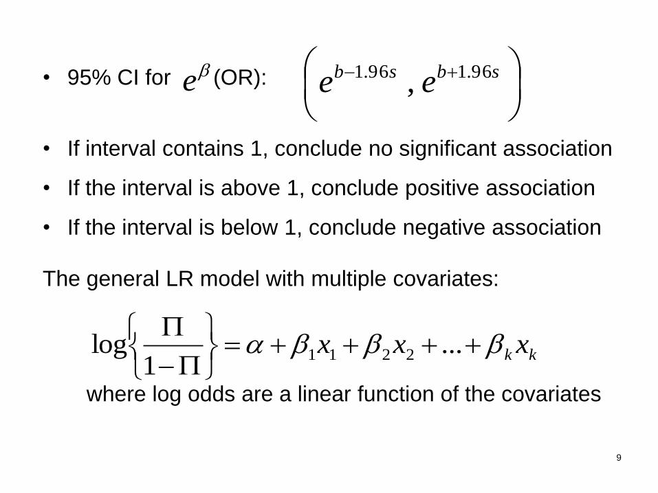
• 95% CI for (OR):

• If interval contains 1, conclude no significant association

• If the interval is above 1, conclude positive association

• If the interval is below 1, conclude negative association

The general LR model with multiple covariates:

where log odds are a linear function of the covariates

sbsb ee 96.196.1 ,e

kk xxx

...

1log 2211

10

Disease Exposure Total

Present Absent

Present a b a+b

Absent c d c+d

Total a+c b+d a+b+c+d

Odds ratio (OR) is the ratio of the odds of exposure in

those with disease to those without

The away from one (in either direction) the stronger the

association with OR = 1 representing no association

OR > 1 ► positive association between D & E

OR < 1 ► negative association between D & E

bc

ad

dc

baOR

/

/

Odds Ratio

11

Chi-square test examines the magnitude of discrepancy between observed frequencies (obs) and expected frequencies (exp)

It measures the significance of association between two categorical variables

Ho : The two (categorical) variables are independent

The test statistic is defined as:

with degrees of freedom (r-1)(c-1)

If p<0.05, reject the hypothesis of independence; i.e. the two (categorical) variables are significantly associated

Chi-square

exp

exp)( 22 obs

12

Let’s consider an example where we are interested in

examining factors associated with low birth-weight

(<2500gm), using a (Stata) dataset lbw.dta. This dataset

contains data from 189 mothers on a number of variables,

including birthweight of newborn, mother’s age, race,

smoking during pregnancy, premature birth history,

hypertension, uterine irritability, visits to physicians....

To load lbw.dta from the web, type the Stata command:

use http://www.stata-press.com/data/r10/lbw,

clear

Working Examples

13

To learn more about contents of the data file, type:

describe

Sorted by: bwt int %8.0g birthweight (grams)ftv byte %8.0g visits to physician during 1st trimesterui byte %8.0g presence, uterine irritabilityht byte %8.0g has history of hypertensionptl byte %8.0g premature labor history (count)smoke byte %8.0g smoked during pregnancyrace byte %8.0g race racelwt int %8.0g weight at last menstrual periodage byte %8.0g age of motherlow byte %8.0g birthweight<2500gid int %8.0g identification code variable name type format label variable label storage display value size: 3,402 (99.7% of memory free) vars: 11 5 Nov 2009 12:32 obs: 189 Hosmer & Lemeshow dataContains data from F:\Workshops\lbw.dta

14

To learn more about a categorical variable (e.g. race), type:

codebook race

To summarize continuous variables (age, lwt), type

sum age lwt

To look at the first 5 cases of some selected variables, type:

list id low age race smoke in 1/5

67 3 other 26 2 black 96 1 white tabulation: Freq. Numeric Label

unique values: 3 missing .: 0/189 range: [1,3] units: 1

label: race type: numeric (byte)

lwt 189 129.8201 30.57515 80 250 age 189 23.2381 5.298678 14 45 Variable Obs Mean Std. Dev. Min Max

15

Suppose we want

• to investigate whether smoking during pregnancy (smoke) is associated with low

birthweight (<2500g) of newborn (low)

• to identify factors associated with low

birthweight of newborn

Research Questions

16

Let’s first look at the frequencies of outcome (low) and

study factor (smoke):

tab1 low smoke

Here, 0=No, 1=Yes

Total 189 100.00 1 59 31.22 100.00 0 130 68.78 68.78 <2500g Freq. Percent Cum.birthweight

-> tabulation of low

Total 189 100.00 1 74 39.15 100.00 0 115 60.85 60.85 pregnancy Freq. Percent Cum. during smoked

-> tabulation of smoke

Data Exploration

17

To examine the relationship, let’s construct a 2x2 table

tab2 smoke low, row exp chi2

Odds Ratio: 0219.22944

3086

db

caOR

Pearson chi2(1) = 4.9237 Pr = 0.026

68.78 31.22 100.00 130.0 59.0 189.0 Total 130 59 189 59.46 40.54 100.00 50.9 23.1 74.0 1 44 30 74 74.78 25.22 100.00 79.1 35.9 115.0 0 86 29 115 pregnancy 0 1 Total during birthweight<2500g smoked

row percentage expected frequency frequency Key

18

• The outcome variable needs to be coded as 0 & 1

0 as reference category (e.g. 0=normal weight) and

1 as the event of interest (e.g. 1=low birth weight)

• Stata has two commands to perform logistic regression

logistic (default output with odds ratios)

logit (default output with coefficients)

LR in Stata

19

logit low smoke

Here OR =

_cons -1.087051 .2147299 -5.06 0.000 -1.507914 -.6661886 smoke .7040592 .3196386 2.20 0.028 .0775791 1.330539 low Coef. Std. Err. z P>|z| [95% Conf. Interval]

Log likelihood = -114.9023 Pseudo R2 = 0.0207 Prob > chi2 = 0.0274 LR chi2(1) = 4.87Logistic regression Number of obs = 189

021943545.27040592.0 ee

smoke 2.021944 .6462912 2.20 0.028 1.080668 3.783083 low Odds Ratio Std. Err. z P>|z| [95% Conf. Interval]

Log likelihood = -114.9023 Pseudo R2 = 0.0207 Prob > chi2 = 0.0274 LR chi2(1) = 4.87Logistic regression Number of obs = 189

logistic low smoke

20

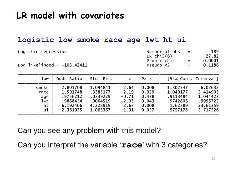
logistic low smoke race age lwt ht ui

Can you see any problem with this model?

Can you interpret the variable ‘race’ with 3 categories?

ui 2.361925 1.065367 1.91 0.057 .9757178 5.717526 ht 6.192406 4.228919 2.67 0.008 1.62389 23.61359 lwt .9868454 .0064519 -2.03 0.043 .9742806 .9995722 age .9756212 .0339229 -0.71 0.478 .9113484 1.044427 race 1.591748 .3385177 2.19 0.029 1.049177 2.414903 smoke 2.801708 1.094841 2.64 0.008 1.302547 6.02632 low Odds Ratio Std. Err. z P>|z| [95% Conf. Interval]

Log likelihood = -103.42411 Pseudo R2 = 0.1186 Prob > chi2 = 0.0001 LR chi2(6) = 27.82Logistic regression Number of obs = 189

LR model with covariates

21

• To accommodate categorical variable race, we need to

include indicator (dummy) variables for race

xi: logistic low smoke i.race age lwt ht ui

ui 2.448163 1.097945 2.00 0.046 1.016474 5.896367 ht 6.401179 4.408588 2.70 0.007 1.659681 24.68853 lwt .9838766 .0067461 -2.37 0.018 .970743 .9971879 age .9818813 .0347117 -0.52 0.605 .9161512 1.052327 _Irace_3 2.465253 1.070712 2.08 0.038 1.052365 5.77506 _Irace_2 3.596888 1.894271 2.43 0.015 1.281294 10.0973 smoke 2.794192 1.100642 2.61 0.009 1.291115 6.047107 low Odds Ratio Std. Err. z P>|z| [95% Conf. Interval]

Log likelihood = -101.98506 Pseudo R2 = 0.1308 Prob > chi2 = 0.0001 LR chi2(7) = 30.70Logistic regression Number of obs = 189

i.race _Irace_1-3 (naturally coded; _Irace_1 omitted)

22

• Prob>chi2=0.0001 ► the model as a whole is

statistically significant (p<0.0001)

• Pseudo R2=0.13 ► McFadden pseudo R2 which can be

interpreted as an approximate amount of variability

explained by the fitted model (with caution!!!)

• ORsmoke=2.79 (p=0.009) ► the odds of having an

underweight baby are increased by a factor of 2.79 for

being smoker (during pregnancy) rather than non-smoker,

controlling for other variables in the model

• ORlwt=0.98 (p=0.018) ► the odds of having an

underweight baby would change by a factor of 0.98 for

every pound increase in weight at last menstrual period,

controlling for other variables in the model

Interpretations

23

• To examine multicollinearity, type:

collin smoke race age lwt ht ui

Det(correlation matrix) 0.7192 Eigenvalues & Cond Index computed from scaled raw sscp (w/ intercept) Condition Number 17.6263 --------------------------------- 7 0.0143 17.6263 6 0.0398 10.5528 5 0.1539 5.3662 4 0.6168 2.6807 3 0.7387 2.4494 2 1.0044 2.1006 1 4.4321 1.0000--------------------------------- Eigenval Index Cond

Mean VIF 1.12---------------------------------------------------- ui 1.04 1.02 0.9627 0.0373 ht 1.08 1.04 0.9296 0.0704 lwt 1.15 1.07 0.8716 0.1284 age 1.07 1.03 0.9339 0.0661 race 1.22 1.10 0.8219 0.1781 smoke 1.16 1.08 0.8606 0.1394---------------------------------------------------- Variable VIF VIF Tolerance Squared SQRT R-

Collinearity Diagnostics

No concern with

multicollinearity

Multicollinearity

24

Model specification

This can be tested by using linktest

linktest

• Insignificant _hatsq (p=0.60) ► the link function is

correctly specified (no specification error)

• Significant _hatsq means either we have omitted relevant

variables or the link function is not correctly specified

_cons .022908 .2214007 0.10 0.918 -.4110295 .4568454 _hatsq -.0915845 .1746935 -0.52 0.600 -.4339775 .2508085 _hat .8791094 .3013084 2.92 0.004 .2885559 1.469663 low Coef. Std. Err. z P>|z| [95% Conf. Interval]

Log likelihood = -101.84316 Pseudo R2 = 0.1320 Prob > chi2 = 0.0000 LR chi2(2) = 30.99Logistic regression Number of obs = 189

LR Diagnostics (post-estimation)

25

Goodness-of-fit

Are the data fit the logistic model well?

• For Hosmer-Lemeshow goodness of fit statistic, type:

lfit, group(10)

► Insignificant p-value (0.1789) suggests that the model

fits the data reasonably well

• To produce other measures of model fit, type:

fitstat

Prob > chi2 = 0.1789 Hosmer-Lemeshow chi2(8) = 11.42 number of groups = 10 number of observations = 189

(Table collapsed on quantiles of estimated probabilities)

Logistic model for low, goodness-of-fit test

26

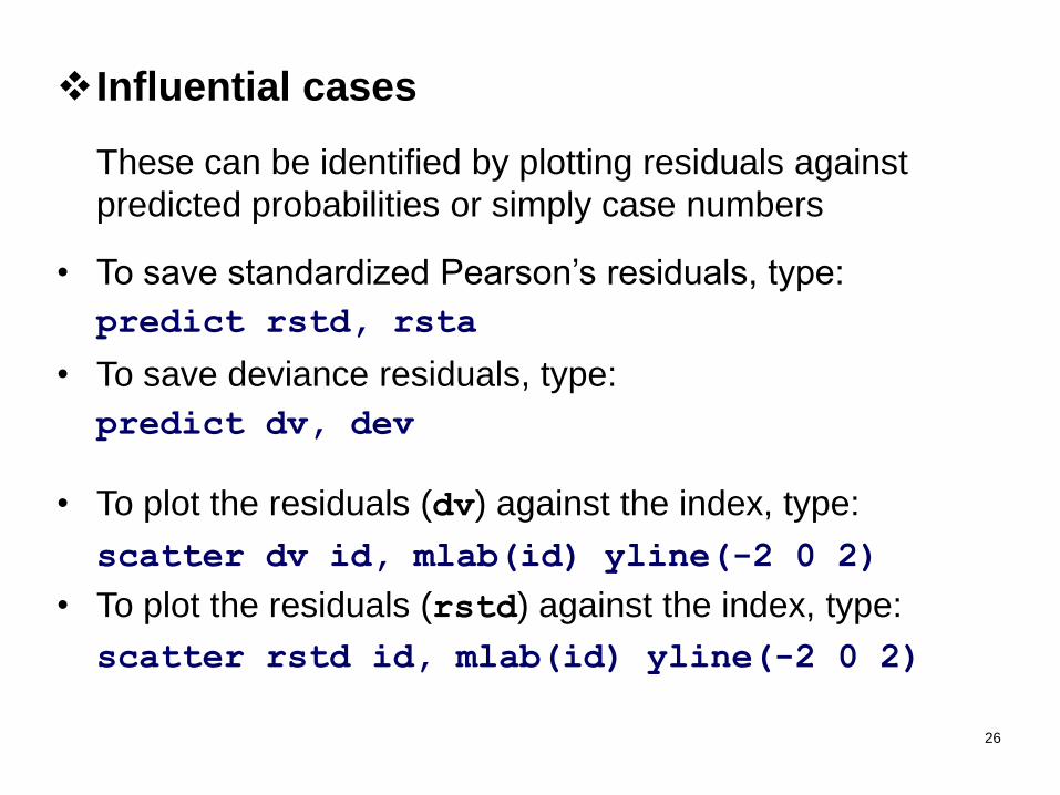
Influential cases

These can be identified by plotting residuals against

predicted probabilities or simply case numbers

• To save standardized Pearson’s residuals, type:

predict rstd, rsta

• To save deviance residuals, type:

predict dv, dev

• To plot the residuals (dv) against the index, type:

scatter dv id, mlab(id) yline(-2 0 2)

• To plot the residuals (rstd) against the index, type:

scatter rstd id, mlab(id) yline(-2 0 2)

27

scatter rstd id, mlab(id) yline(-2 0 2)

• You can identify influential cases by typing:

list rstd id if abs(rstd)> 2

list dv id if abs(dv)> 2

108 207173175112 183 223129 204120 191114 131 217169151 195190185 221182174134 220184 215126

22522292 136 219196203200 213218145168

139 186

226211

179 21286 97 12391 214149 177135 156 201125 209109 12410394 105

170142 20895 162

44

224106

146161

181 205

159

176113206

87

1601439396

127130118 216

14067

141210

121 193192150 199

82

155

3723 50

107

4 61 7840

148147154163

60

30 6952

128

13

76

17

47

15

63

111

34

115 166

46

84

24 35

104189167

164

26

51

83

3254

85

45

180

6242

68

19

31

79

88

81

99

11

102

89

25

100101188

27

56

29

202187

137172

65

20

22

4916

75

7118

43

36

33

197138119

59

144

57

117116

10

77

28

98 132133-2-1

01

23

sta

nd

ard

ize

d P

ea

rson r

esid

ual

0 50 100 150 200 250identification code

28

• Influential cases can also be identified by examining

Pregibon leverage or Pregibon’s Delta-Beta influential

statistic

• To save Pregibon leverage, type

predict hat, hat

• To save Pregibon’s dbeta, type

predict pgbon, dbeta

• You can identify influential cases by typing:

list pgbon id if pgbon>0.2

• To plot dbeta against the index, type

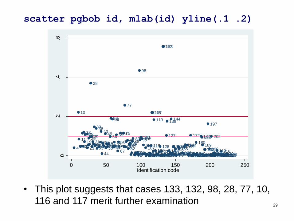
scatter pgbon id, mlab(id) yline(.1 .2)

29

121

221208

17

134

14762

99

98

22021997 181

46

215

19

213

155

156130

106207

6324

174

138

201143196

5415

223173129

71

30

214177185

32

36

199

43

222139 184176

107

168

33

49

20092 203146

10

186

111

161204

160

25

212206

52

114216

102

210190

3147

81

226225175

166

136 191108109 135131120

104

19591 217183

76

218

85

117

57

1816

28

93 14996

20275

83

11286 145 179169142

116

150

182151

13 148

7968

23167163

132

26 45

170

35

89

11337

95

60

65

197

44 224

1891645169

19382

100

84

137

119

127

3450 192

18818729 56

180

205162123

154

94

144

4

105141140

17227

59

6140

20

67159

11

124

42

118103

78 115

209211126

133

101

128

77

22

87

88

1250.2

.4.6

Pre

gib

on

's d

be

ta

0 50 100 150 200 250identification code

scatter pgbob id, mlab(id) yline(.1 .2)

• This plot suggests that cases 133, 132, 98, 28, 77, 10,

116 and 117 merit further examination

30

Assumption of linearity

• To assess whether log odds of the outcome is linearly

associated with the covariates, Lowes graph can be

produced by typing:

predict pr

lowess low pr, addplot(function y=x, leg(off))

0.2

.4.6

.81

bir

thw

eig

ht<

250

0g

0 .2 .4 .6 .8 1Pr(low)

bandwidth = .8

Lowess smoother

Reasonably

linear relationship

31

• To run a backward stepwise logistic model, type

xi: sw, pr(0.05): logistic low smoke

(i.race) age lwt ht ui

• To run a forward stepwise logistic model, type

xi: sw, pe(0.05): logistic low smoke

(i.race) age lwt ht ui

ht 6.490237 4.483259 2.71 0.007 1.676009 25.13302 lwt .9834361 .0066887 -2.46 0.014 .9704134 .9966336 ui 2.471801 1.106213 2.02 0.043 1.028189 5.942297 _Irace_3 2.526023 1.087054 2.15 0.031 1.08675 5.871446 _Irace_2 3.758631 1.959795 2.54 0.011 1.352705 10.44375 smoke 2.817403 1.105908 2.64 0.008 1.305356 6.080917 low Odds Ratio Std. Err. z P>|z| [95% Conf. Interval]

Log likelihood = -102.11978 Pseudo R2 = 0.1297 Prob > chi2 = 0.0000 LR chi2(6) = 30.43Logistic regression Number of obs = 189

p = 0.6050 >= 0.0500 removing age begin with full modeli.race _Irace_1-3 (naturally coded; _Irace_1 omitted)

Stepwise Logistic Regression

32

Fitting other LR Models

• Polytomous outcome (choice of rehabilitation:

home/clinic/nursing home/hospital)

Multinomial (polytomous) logistic regression

Stata command:

mlogit choice gender age .......

• Ordered outcome (physical activity: none, low,

moderate, vigorous)

Ordinal logistic regression

Stata command:

ologit satis gender age .......

33

Some References

Logistic Regression

• Hosmer DW, Lemeshow SL (2000) Applied Logistic

Regression. 2nd edition, Wiley-Interscience.

• Hilbe JM (2009) Logistic Regression Models. 1st edition,

Chapman & Hall/CRC

• Long JS, Freese J (2006) Regression Models for Categorical

Dependent Variables Using Stata, 2nd edition, Stata Press

Introductory Stata

• Acock A (2008) A Gentle Introduction to Stata, 2nd edition,

Stata Press

• Juul S (2008) An Introduction to Stata for Health

Researchers, 2nd edition, Stata Press

34

Getting Help

Within Stata:

• To get help in a particular command (e.g. regression)

help regression

• To obtain all references to a topic (e.g. logistic)

search logistic

• To find relevant commands on a topic (e.g. anova)

findit anova

Online Stata support : www.stata.com/support

AU/NZ distributor for Stata & StatTransfer

www.survey-design.com.au

– Stata GradPlan arrangements for students

35

Thank you

Comments

Questions?