MODE CHOICE MODEL FORDOMESTIC TOURIST TRAVEL

PRESENTED BY:NAINA GUPTA

GUIDED BY:MR.PRASANTH VARDHAN

MR.BHASKAR GOWD SUDAGANI

STRUCTURE OF PRESENTATION• Introduction• Case Study Description• Mode Choice Models

– Binary Logit Model• Model Development

– Parameters Identification– Generalized Cost– Model I: Taxi vs HOHO– Model II: Taxi vs City Bus

• Model Sensitivity• Conclusions• Way Forward

INTRODUCTION• Traffic and transportation in Indian cities is not

encouraging tourists towards public transport.• To alleviate the situation, this research highlight the

travel behavior and mode choice of tourist.• Decision making behavior of the tourists has been

understood by studying the attributes of travelcharacteristics.

• Attempt has been made to address the situationusing the concept of mode choice model.

CASE STUDY DESCRIPTION• 7 tourist locations, were identified within Delhi by

considering the past tourism statistics of thoselocations, published by the Ministry of Tourism*(Qutub Minar,Red Fort,Humayun's Tomb,Jama Masjid,Bahaitemple,Akshardham,Pragati Maidan)

• 21 lakhs* domestic tourists are attracted in the citywith an average daily arrival of 6000 tourists.

• Tourist opinion survey has been conducted with asample of 163 tourist groups comprising 499people’s characteristics, accounting to 8.4 % of dailytourist inflow.

* Source: India Tourism Statistics,2014

MODE CHOICE MODELMode choice

models

Logit Model

Binary Logit Nested LogitModel

MultinomialLogit Model

Probit ModelGeneralized

Extreme ValueModel

Binary Logit Model hasbeen used as a tool forthe research to developrelationship betweenmode & influencingparameters.

BINARY LOGIT

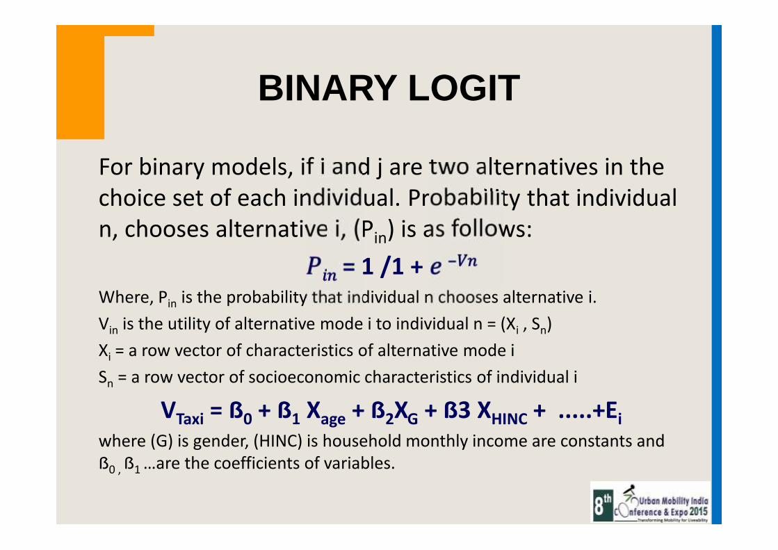
For binary models, if i and j are two alternatives in thechoice set of each individual. Probability that individualn, chooses alternative i, (Pin) is as follows:

= 1 /1 + −

Where, Pin is the probability that individual n chooses alternative i.Vin is the utility of alternative mode i to individual n = (Xi , Sn)Xi = a row vector of characteristics of alternative mode iSn = a row vector of socioeconomic characteristics of individual i

VTaxi = ẞ0 + ẞ1 Xage + ẞ2XG + ẞ3 XHINC + .....+Eiwhere (G) is gender, (HINC) is household monthly income are constants andẞ0 , ẞ1 …are the coefficients of variables.

PARAMETERS IDENTIFICATION

• Based on earlier literature ,18variables, were identified to beused in the calibration process.

• 20 runs for differentcombination of variables werecarried out using logisticregression*.

• Combinations of variablesexhibiting poor statisticalgoodness-of-fit, were rejected.

* SPSS 10 software has been used.

PARAMETERS• Total travel time• In vehicle time• Out vehicle time• Travel cost• In vehicle cost• Out vehicle cost• Waiting time• Distance• Access distance• Dispersal distance• Access cost• Dispersal cost• Vehicle ownership• Duration of stay• Group size• Income• Gender• Age

PARAMETERS IDENTIFICATION• After dropping variables with insignificant coefficients,

the explanatory variables were Age, gender, Income,group size, out vehicle travel time, total travel cost, invehicle time, Wait Time.

• Explanatory variables such as age, monthly income &gender were categorized.

• Gender was categorized as 0 for male & 1 for female.• Age was categorized as <14, 15-24, 25-34,35-44,45-

54,55- 64 and >64.• Income was categorized as 0-20000 Rs.,20000-30000 Rs.,

30000- 40000Rs., 40000-50000 Rs. & > 50000Rs.

GENERALIZED COST• Logistic regression was used to develop utility

equations and the total disutility of travel wasestimated in the form of generalized cost.

• The perceived values associated with in-vehicle traveltime, out- vehicle time, wait time & cost for thestudy were estimated.

According to model for HOHO;U = 3.214 (IVT) – 4.640 (OVT) - 8.249 (WT) + 2.801 (TC)-1.641

Where;TC: Travel Cost in Rs / kmIVT: in-vehicle travel time in minutes / kmOVT: out-vehicle travel time in minutes / kmWT: wait time in minutes / km

GENERALIZED COST

Based on the above utility model developed, the values

of different attributes are estimated as follows:

Value of IVT = 1.14 Rs / minute

Value of OVT = 1.65 Rs / minute

Value of WT = 2.95 Rs / minute

Generalized Cost (in Rs) = 1.14 (IVT) + 1.65 (OVT) + 2.95 (WT) +

Total Travel Cost

MODEL DEVELOPMENT

Binary logit model was developed for two alternatives,

a) Taxi vs HOHO and

b) Taxi vs City Bus.

These are taken to compare the utility of these travel

modes and identify the factors that would influence

users travelling by taxi to move to tourist buses (HOHO)

or city buses.

MODEL 1: TAXI vs HOHO BUSSummary of estimations from binary logit model for Taxi(0) vs HOHO Bus(1)

Negative coefficients for age,income, group size andwaiting time implies that anincrease in value of thesevariables would lower HOHObus usage.

Income is the leastsignificant variable.Most significant variablein the model is waitingtime followed by cost, Invehicle time, age &group size.

UTILITY EQUATION OF CHOOSING HOHO= − 5.520 − 0.478 ∗ −1.108 ∗ −0.575 ∗ − 1.727 ∗

+ 0.090 ∗ ℎ + 0.078 ∗ ℎ −0.235∗+ 0.009 ∗

Probability Curve of Choosing HOHOAge is significant asit implies that oldpeople are lesslikely to use HOHO.

PROBABILITY PREDICTION OF CHOOSING HOHO:= 1/[1 + (−(−5.520 − 0.478 ∗ − 1.108 ∗ − 0.575 ∗ − 1.727 ∗ +

0.090∗ + 0.078 ∗ −0.235∗ +0.009 ∗ ))]Reference forfemale: 1 & male: 0implies that malesare more likely toshift to HOHO.

Group size coefficientreveals that increasein group size wouldreduce probability ofHOHO.

Hosmer & Lemeshow’s goodness-of-fit test statistic

• The -2 log likelihood reflects the prediction deviation(error) by the model which has been observed as188.292.

• The model has:Cox and Snell’s value = 0.533Nagelkerke value = 0.687

Observed & expectedfrequencies did notdiffer considerablydepicting good fitnessof test.

MODEL 2: TAXI vs CITY BUSSummary of estimations from binary logit model for Taxi(0) vs City Bus(1)Negative coefficients for age,

gender, income, in vehicletime and waiting time impliesthat an increase in value ofthese variables would lowercity bus usage.Most significant

variable in the equationis income, followed bywait time, cost, invehicle time and age inaccordance to Waldtest value.UTILITY EQUATION OF CHOOSING CITY BUS:

Vn = −1.543 −0.849∗ − 0.683∗ − 4.332∗ − 1.436∗−0.215∗ - ℎ + 0.226∗ -v ℎ − 0.77∗+0.084∗

PROBABILITY PREDICTION OF CHOOSING CITY BUS:= 1/ (1+ (-(−1.543−0.849∗ −0.683∗ −4.322∗ −1.436∗ −0.215∗ +

0.226∗ −0.77∗ +0.084∗ )))

Probability Curve of Choosing City BusAge is significant asit implies that oldpeople are lesslikely to use HOHO.

Income Coefficientreveals that increasein value woulddecrease probabilityof using city bus

Hosmer & Lemeshow’s goodness-of-fit test statistic

• The -2 log likelihood reflects the prediction deviation(error) by the model which has been observed as52.725 indicating a better fit.

• The model has:Cox and Snell’s value = 0.410Nagelkerke value = 0.841

Observed & expectedfrequencies are veryclose depicting good fitof the model.

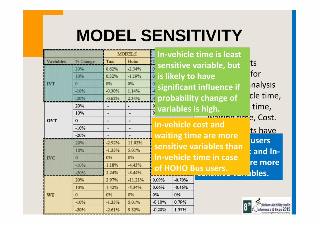
• Model inputsconsidered forsensitivity analysisare: In-vehicle time,Out-vehicle time,waiting time, Cost.

• Model inputs havebeen varied from -20% to +20% toassess the impact.

MODEL SENSITIVITY

In case of bus usersIn-vehicle cost and In-vehicle time are moresensitive variables.

In-vehicle cost andwaiting time are moresensitive variables thanIn-vehicle time in caseof HOHO Bus users.

In-vehicle time is leastsensitive variable, butis likely to havesignificant influence ifprobability change ofvariables is high.

PROBABILITY CURVESProbability curve of HOHO with % changes in disutilityProbability curve of City Bus with % changes in disutility

Probability that anindividual will useHOHO will increaseafter the differencebetween GC of Taxi& HOHO is Rs 420.

Probability of choosingHOHO when all inputvariables decrease by20% will increase afterdifference between GC oftaxi & HOHO is Rs.320.

Probability of choosingHOHO when all inputvariables increase by20% will increase afterdifference between GCof taxi & HOHO isRs.500.

CONCLUSIONS

• Gender, Age and Income variables are contributingsignificantly to explain the mode choice behavior;which is consistent with past researches.

• Most significant variable for choosing HOHO bususers is waiting time followed by cost, In vehicletime, age and group size.

• For Bus users Income is the most significant variablefollowed by wait time, cost, in vehicle time and age.

• Sensitivity analysis reveals that tourists using publictransport are time savers rather than money savers.

• For HOHO users Waiting time and In-vehicle cost aremore sensitive variables.

• With every 20% increase in waiting time there is11.21 % decrease in HOHO as a choice, with every20% reduction probability increases by 9.82%.

• For bus users In-vehicle cost and In-vehicle time aremore sensitive variables.

• With every 20% increase in in-vehicle cost there is1.84 % increase in bus as a choice & for every 20%reduction probability decrease by 3.24%.

CONCLUSIONS

WAY FORWARD

• Similar model can be developed using nested logitmodel or multinomial logit model and can becompared.

• Further, the transferability of model can be checkedto other cities.

REFERENCES1. AHERN, A & TAPLEY, N. 'The use of stated preference techniques to model modal choices on

interurban trips in Ireland' Transportation Research Part , vol.42, no.1, 2008, pp.15-27.2. ANTONIOU, C & TYRINOPOULOS.' Factors Affecting Public Transport Use in Touristic Areas',

International Journal of Transportation,vol.1, no.1,2013, pp.91-112.3. CAN,V. 'Estimation of travel mode choice for domestic tourists to Nha Trang using the

multinomial probit model', Transportation Research Part 12A: Policy and Practice,vol.49,2013, pp.149-159.

4. COSHALL, J. ‘A selection strategy for modeling UK tourism flows by air to Europeandestinations’, Tourism Economics, vol.11, no.4, 2005, pp.141- 158.

5. HSIEH, S,O'LEARY, J, MORRISON, A& CHANG, P. 'Modelling the travel mode choice ofAustralian outbound travellers', Journal of Tourism Studies, vol.4, no.1, 1993,pp.51-61.

6. MINAL & SEKHAR,C. ' Mode choice analysis: the data, the models and future ahead',International Journal for Traffic and Transport Engineering, vol.4, no.3, 2014, pp.269-285

7. PHANI KUMAR, DEBASIS BASU, AND BHARGAB MAITRA, ‘Modeling Generalized Cost of Travelfor Rural Bus Users: A Case Study’, Journal of Public Transportation, Vol. 7, No. 2, 2004

8. SONG,H & LI, G. 'Tourism demand modelling and forecasting—A review of recent research',Tourism Management, vol.29,no.2 ,2008,pp.203-220.

9. VU, C. J., & TURNER, L. ‘Data disaggregation in demand forecasting’, Tourism and HospitalityResearch, vol.6, no.1, 2005, pp.38-52.