mobile ad-hoc networks location prediction by using ... · pdf filemobile ad-hoc networks...

Mobile Ad-hoc Networks Location Prediction by using Artificial Neural

Networks: Considerations and Future Directions

Ammar Yassir1, Gamal Abdel Nasir2, Dr.Priyanka Roy3

Department of Information Technology, CMJ University, Shillong, India1

Faculty of Computer Science and Information Systems, UTM University, Malaysia2

Professor, Gateway Education Pvt Ltd, Chandigarh, India3

Abstract

Location prediction serves to save capacity on the

air interface of mobile radio networks.

Location prediction is the estimation of a mobile

host’s location at a time in future. When the future

location of a mobile host is known, this information

can be used in a number of ways to improve the

performance of the network. The hosts are free to

move anywhere. The mobile hosts can move with different mobility

patterns. Mobility Models are used to represent the

different mobility patterns. Mobility metrics are

used to differentiate the mobility models from each

other. Different mobility models impact the

protocols in different ways.

A selection of neural networks of the feed-forward

and feedback type are examined to prove their

suitability for this purpose. In this paper, as first

results preferable network structures, input vectors,

learning parameters and the simulated prediction

probabilities are presented. A comparison with

conventional methods shows the advantages and

disadvantages of the use of neural networks for

motion prediction. The results show that the gain

depends on the user profile and the amount of

extraordinary movements of the subscriber.

Keywords—Location Prediction, Mobile hosts,

neural networks, Mobility metrics, MANET

I. INTRODUCTION

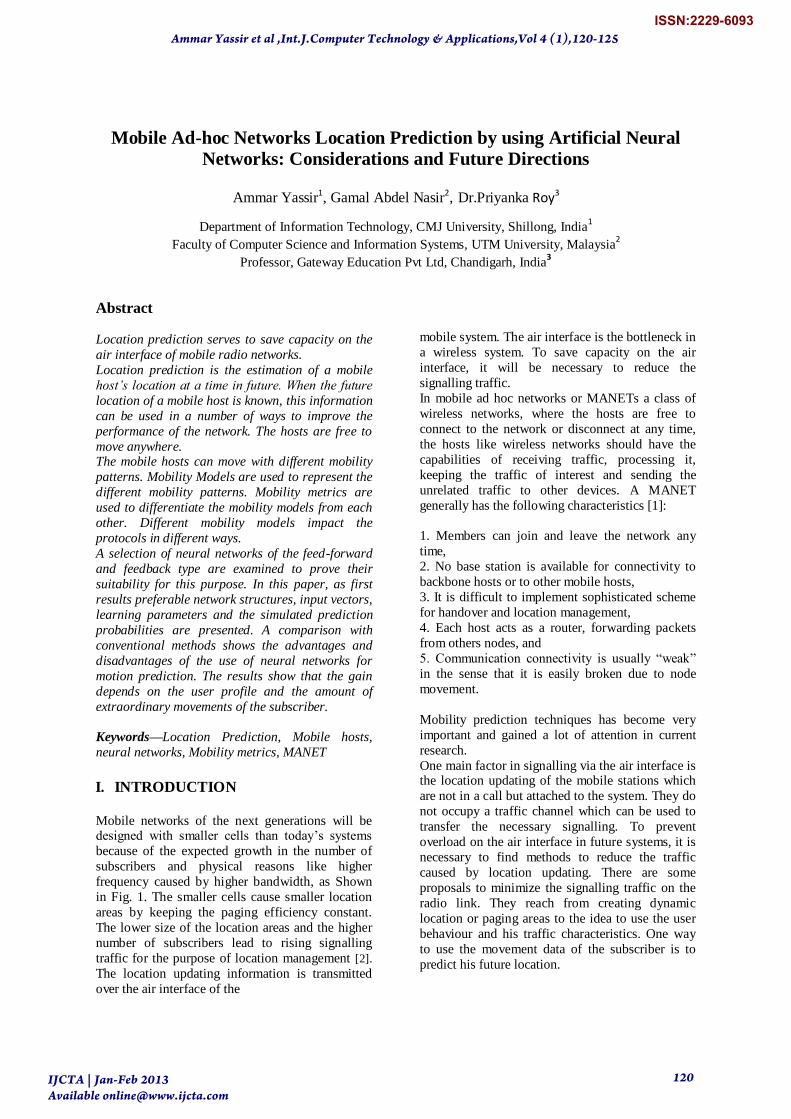
Mobile networks of the next generations will be designed with smaller cells than today‟s systems

because of the expected growth in the number of

subscribers and physical reasons like higher

frequency caused by higher bandwidth, as Shown

in Fig. 1. The smaller cells cause smaller location

areas by keeping the paging efficiency constant.

The lower size of the location areas and the higher

number of subscribers lead to rising signalling

traffic for the purpose of location management [2].

The location updating information is transmitted

over the air interface of the

mobile system. The air interface is the bottleneck in

a wireless system. To save capacity on the air

interface, it will be necessary to reduce the

signalling traffic.

In mobile ad hoc networks or MANETs a class of

wireless networks, where the hosts are free to

connect to the network or disconnect at any time,

the hosts like wireless networks should have the

capabilities of receiving traffic, processing it,

keeping the traffic of interest and sending the

unrelated traffic to other devices. A MANET

generally has the following characteristics [1]:

1. Members can join and leave the network any

time,

2. No base station is available for connectivity to

backbone hosts or to other mobile hosts,

3. It is difficult to implement sophisticated scheme

for handover and location management,

4. Each host acts as a router, forwarding packets

from others nodes, and

5. Communication connectivity is usually “weak”

in the sense that it is easily broken due to node

movement.

Mobility prediction techniques has become very

important and gained a lot of attention in current

research.

One main factor in signalling via the air interface is the location updating of the mobile stations which

are not in a call but attached to the system. They do

not occupy a traffic channel which can be used to

transfer the necessary signalling. To prevent

overload on the air interface in future systems, it is

necessary to find methods to reduce the traffic

caused by location updating. There are some

proposals to minimize the signalling traffic on the

radio link. They reach from creating dynamic

location or paging areas to the idea to use the user

behaviour and his traffic characteristics. One way

to use the movement data of the subscriber is to

predict his future location.

Ammar Yassir et al ,Int.J.Computer Technology & Applications,Vol 4 (1),120-125

IJCTA | Jan-Feb 2013 Available [email protected]

120

ISSN:2229-6093

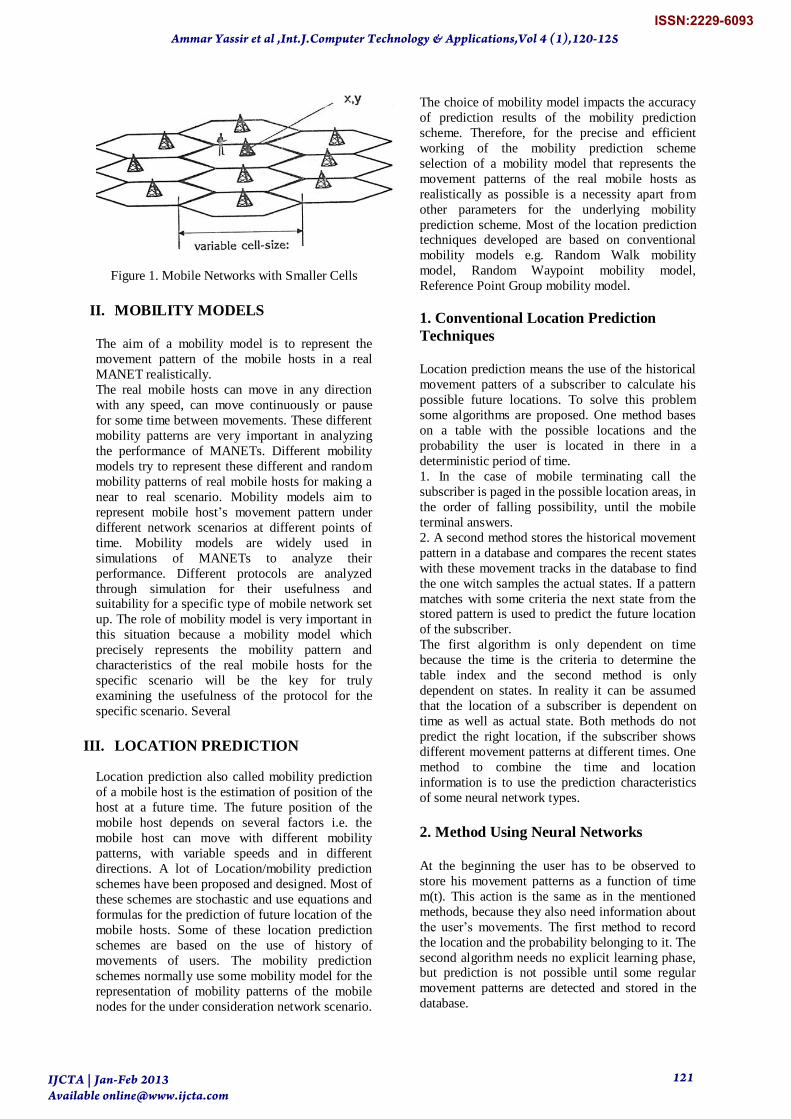
Figure 1. Mobile Networks with Smaller Cells

II. MOBILITY MODELS

The aim of a mobility model is to represent the

movement pattern of the mobile hosts in a real

MANET realistically.

The real mobile hosts can move in any direction

with any speed, can move continuously or pause

for some time between movements. These different

mobility patterns are very important in analyzing

the performance of MANETs. Different mobility

models try to represent these different and random

mobility patterns of real mobile hosts for making a

near to real scenario. Mobility models aim to

represent mobile host‟s movement pattern under

different network scenarios at different points of

time. Mobility models are widely used in

simulations of MANETs to analyze their

performance. Different protocols are analyzed

through simulation for their usefulness and suitability for a specific type of mobile network set

up. The role of mobility model is very important in

this situation because a mobility model which

precisely represents the mobility pattern and

characteristics of the real mobile hosts for the

specific scenario will be the key for truly

examining the usefulness of the protocol for the

specific scenario. Several

III. LOCATION PREDICTION

Location prediction also called mobility prediction

of a mobile host is the estimation of position of the

host at a future time. The future position of the

mobile host depends on several factors i.e. the

mobile host can move with different mobility

patterns, with variable speeds and in different

directions. A lot of Location/mobility prediction

schemes have been proposed and designed. Most of

these schemes are stochastic and use equations and

formulas for the prediction of future location of the

mobile hosts. Some of these location prediction

schemes are based on the use of history of

movements of users. The mobility prediction

schemes normally use some mobility model for the

representation of mobility patterns of the mobile

nodes for the under consideration network scenario.

The choice of mobility model impacts the accuracy

of prediction results of the mobility prediction

scheme. Therefore, for the precise and efficient

working of the mobility prediction scheme

selection of a mobility model that represents the

movement patterns of the real mobile hosts as

realistically as possible is a necessity apart from

other parameters for the underlying mobility

prediction scheme. Most of the location prediction techniques developed are based on conventional

mobility models e.g. Random Walk mobility

model, Random Waypoint mobility model,

Reference Point Group mobility model.

1. Conventional Location Prediction

Techniques

Location prediction means the use of the historical

movement patters of a subscriber to calculate his

possible future locations. To solve this problem

some algorithms are proposed. One method bases

on a table with the possible locations and the

probability the user is located in there in a

deterministic period of time.

1. In the case of mobile terminating call the

subscriber is paged in the possible location areas, in

the order of falling possibility, until the mobile

terminal answers.

2. A second method stores the historical movement

pattern in a database and compares the recent states

with these movement tracks in the database to find

the one witch samples the actual states. If a pattern

matches with some criteria the next state from the stored pattern is used to predict the future location

of the subscriber.

The first algorithm is only dependent on time

because the time is the criteria to determine the

table index and the second method is only

dependent on states. In reality it can be assumed

that the location of a subscriber is dependent on

time as well as actual state. Both methods do not

predict the right location, if the subscriber shows

different movement patterns at different times. One

method to combine the time and location

information is to use the prediction characteristics

of some neural network types.

2. Method Using Neural Networks

At the beginning the user has to be observed to

store his movement patterns as a function of time

m(t). This action is the same as in the mentioned

methods, because they also need information about

the user‟s movements. The first method to record

the location and the probability belonging to it. The

second algorithm needs no explicit learning phase, but prediction is not possible until some regular

movement patterns are detected and stored in the

database.



121

ISSN:2229-6093

In the next step the suitable neural network has to

be trained with the observed motion pattern m(t).

After training the network the recall phase is used

for prediction. The actual movement and time is

used to feed the neural network and to get the

output the next location or locations depending on

the output vector. We expect from this method that

it shows better results with unknown movements

than the conventional methods, but the same results with known movements.

3. Subscriber Profile

The movement pattern function m(t) is a discrete

function, it consists of samples {m(ti)}. The time

intervals ti-ti-1 may be constant or non-constant

depending on the recording method. The first

method is to register each location update

generated from the mobile terminal when changing the location area. The location update messages

arrive in non-deterministic times. The second

variant takes samples in constant time intervals by

looking in the networks location table as Shown in

Fig 2.

.

Figure 2. Subscriber Profile (Example)

In this examination we use only constant time

intervals to build the user profile. A mobile

network with 20 location areas was chosen,

numbered from 1 to 20. We constructed a

subscriber‟s movement pattern, as shown in Fig 2,

in this exemplary mobile network by writing down

the locations regularly six times a day for four

weeks, which means we obtain 168 location values. The sample rate may be higher depending on the

subscribers‟ movement and location area size. The

absolute time values, e.g. days and weeks, don‟t

constitute a restriction of the generality. With these

order of location area numbers, transformed into a

set of input and output patterns, we carried out our

investigations.

IV. INPUT AND OUTPUT VECTORS

Wherever Times is specified, Times Roman or

Times New Roman may be used. If neither is

available on your word processor, please use the

font closest in appearance to Times. Avoid using

bit-mapped fonts if possible. True-Type 1 fonts are

preferred.

1. Contents

The contents of the input and output vector depends

one the neural network type and on our different

studies to find a relation between prediction output

and contents of the vectors. Feedback neural

networks have the ability to remember the order in

which the input patterns are presented during the

training, because of their backward connections.

With these networks, it is only necessary to give

the last known location area number l as input

vector (1).

i = (l); l =1, 2, ..., 20 (1)

Feed-forward neural networks are memory-less, that means their output is independent of the

previous inputs. For this neural network

architecture a modified input vector is appropriate.

One possibility is the presentation of the N last

known locations (2). N has to be varied in our

examination, to get the best prediction

probabilities.

i = ( li, li-1 ,...,li-N ); l = 1, 2, ..., 20 (2)

In addition to the last known locations of the

subscriber, other information can be given to the

neural network. For example, we considered the

absolute time, in form of a couple of day and hour

(3). This information may be useful, because it may

be correlated with the subscriber habits. The time

information in the input vector is useful with both

types of neural networks.

i = ( li, li-1 ,...,li-N , t ); l = 1, 2, ..., 20 (3) The output-information is another important topic.

We want to obtain as output information only the

location area number, in our example a value

between 1 and L. The time information is not

necessary in the output vector because we studied

only a prediction for the next time interval t+Dt. If

the prediction should be extended to the prediction

of the location at the time t+kDt the time

information has to be included in the input vector.

A second information which will be useful in the

output vector are the probabilities that the

subscriber is located in the predicted location areas.

2. Encoding Of The Input And Output

An input pattern is a set of activation values of the

neurones belonging to the input layer of the neural network. The conversion of the real data into the

input pattern is called encoding [3]. There are

several possibilities to present the input data to the

neural network in an appropriate form. We studied

the quasi-continuous and the binary coding.



122

ISSN:2229-6093

Quasi-continuous representation means the real

input data, e.g. location area number and time, are

encoded with rational values in a certain interval,

e.g. [0;1] in steps of (1/l). In this configuration the

neural networks can be building with only one

neurone in the input layer.

Binary encoding means the real input data are

encoded with the values „0‟ and „1‟. In this case the

amount of neurones in the input layer is equal to the amount of location areas plus the time values

for one period. For this reason the total number of

neurones in the input layer rises with the size of the

modeled mobile network and the sample rate of the

subscriber movement function in case of binary

encoding.

The encoding of the output vector corresponds to

the encoding of the input vector, with the

difference that the time has not to be considered.

Binary encoding of the output information means

the predictions consists of one or more location

area numbers without any probability information

[4]. Whereas quasi continuous encoding is able to

deliver probability information corresponding to

the predicted location area number. This

information can be used for multiple paging

attempts. The disadvantage of this output layer structure is that each location area number needs to

be coded with one output neurone.

Following the multiple paging method is described.

The mobile system first pages the location area

corresponding to the neurone with the greatest

activation value. If the subscriber does not respond

to the paging, the system tries the location areas

corresponding to the next activation values in order

of falling activation, until the subscriber is found or

a maximal number of attempts are reached.

V. EXAMINED NEURAL NETWORK

ARCHITECTURES

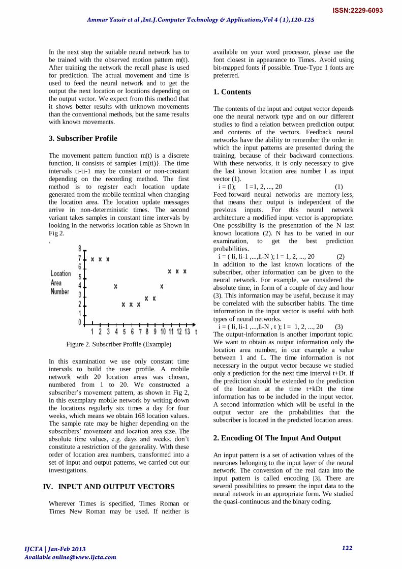
Representing the feedback type we chose Jordan-,

Elman- and Hierarchical Elman-Networks, as

shown in fig 3, and additionally we examined

different feed forward networks structures. The

learning algorithms studied were the standard back-

propagation algorithm, back propagation with

momentum term, quick prop and resilient

propagation [5].

The first step of the examination was the

determination of the best specific network

parameters, like learning, updating and initializing

parameters. To avoid complicating the

investigations, no input or site functions have been

used, and neither activation nor output functions

have been changed during the simulation. We

chose the tangents hyperbolic function as activation and the identity function as output function.

Figure 3. Examined Neural Networks Architectures

The testing of Hierarchical Elman networks did not

show better results than Elman networks, for this

reason we did not incorporate them in the further

investigations. The simulations support the results

from the Elman networks.

The next neural network structure studied was the

Jordan network type. Rising amount of neurones in the hidden layer improves the results in this case.

The other result, like learning with resilient

propagation, binary coding and including time

information, from Elman networks are confirmed.

The simulation with the same variation of

parameters showed no significant differences to the

results of the Elman networks.

Feed-forward networks delivered the following

results. The consideration of time in the input

vector is very important to gain sufficient

prediction results. Higher amount of neurones in

the hidden layer improves the prediction. The best

learning algorithm was back propagation with

momentum term, the obtained results improved

with rising of N, the last known locations in the

input vector.

In our examination feed-forward networks delivered better results than the feedback networks

with the chosen input vector and amount of training

data. This is an unexpected result that suggests to

use other input data and other learning algorithms

in future. The feed-forward networks produce

better results with more neurones in the hidden

layer. The best learning rule back-propagation with

momentum term showed better generalization

results with a rising number of historical states in

the input vector.

At last we trained then the best neural network for

20000 learning epochs in order to test it with new

profiles in the recall phase.

VI. PREDICTION RESULTS

After the training of the best feed-forward network,

we tested it in the recall phase with changed

profiles. The first profiles were a one day and the

second a half-day shifting of the original subscriber



123

ISSN:2229-6093

profile on the time axis. An second studied case

was a non-moving mobile station in a previously

visited location area. First results are promising;

they showed correct prediction probabilities around

80% within three paging attempts.

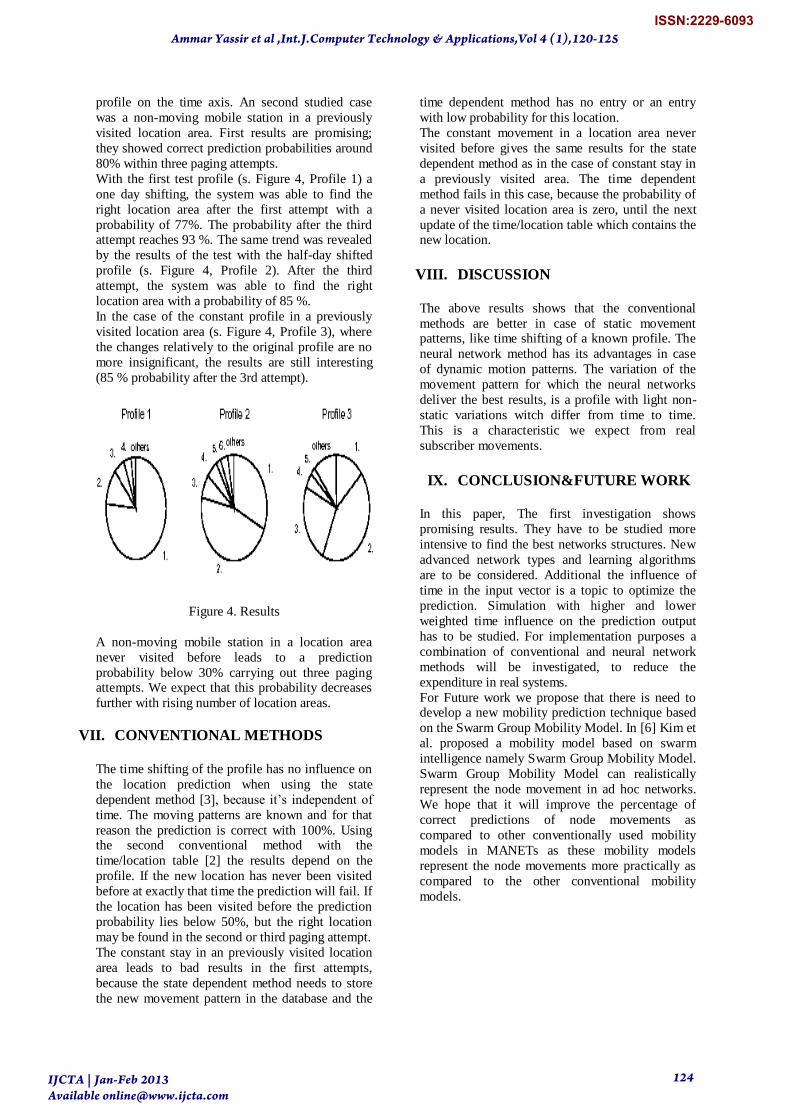
With the first test profile (s. Figure 4, Profile 1) a

one day shifting, the system was able to find the

right location area after the first attempt with a

probability of 77%. The probability after the third attempt reaches 93 %. The same trend was revealed

by the results of the test with the half-day shifted

profile (s. Figure 4, Profile 2). After the third

attempt, the system was able to find the right

location area with a probability of 85 %.

In the case of the constant profile in a previously

visited location area (s. Figure 4, Profile 3), where

the changes relatively to the original profile are no

more insignificant, the results are still interesting

(85 % probability after the 3rd attempt).

Figure 4. Results

A non-moving mobile station in a location area

never visited before leads to a prediction

probability below 30% carrying out three paging attempts. We expect that this probability decreases

further with rising number of location areas.

VII. CONVENTIONAL METHODS

The time shifting of the profile has no influence on

the location prediction when using the state

dependent method [3], because it‟s independent of

time. The moving patterns are known and for that

reason the prediction is correct with 100%. Using the second conventional method with the

time/location table [2] the results depend on the

profile. If the new location has never been visited

before at exactly that time the prediction will fail. If

the location has been visited before the prediction

probability lies below 50%, but the right location

may be found in the second or third paging attempt.

The constant stay in an previously visited location

area leads to bad results in the first attempts,

because the state dependent method needs to store

the new movement pattern in the database and the

time dependent method has no entry or an entry

with low probability for this location.

The constant movement in a location area never

visited before gives the same results for the state

dependent method as in the case of constant stay in

a previously visited area. The time dependent

method fails in this case, because the probability of

a never visited location area is zero, until the next

update of the time/location table which contains the new location.

VIII. DISCUSSION

The above results shows that the conventional

methods are better in case of static movement patterns, like time shifting of a known profile. The

neural network method has its advantages in case

of dynamic motion patterns. The variation of the

movement pattern for which the neural networks

deliver the best results, is a profile with light non-

static variations witch differ from time to time.

This is a characteristic we expect from real

subscriber movements.

IX. CONCLUSION&FUTURE WORK

In this paper, The first investigation shows

promising results. They have to be studied more

intensive to find the best networks structures. New

advanced network types and learning algorithms

are to be considered. Additional the influence of

time in the input vector is a topic to optimize the

prediction. Simulation with higher and lower

weighted time influence on the prediction output

has to be studied. For implementation purposes a

combination of conventional and neural network

methods will be investigated, to reduce the

expenditure in real systems.

For Future work we propose that there is need to develop a new mobility prediction technique based

on the Swarm Group Mobility Model. In [6] Kim et

al. proposed a mobility model based on swarm

intelligence namely Swarm Group Mobility Model.

Swarm Group Mobility Model can realistically

represent the node movement in ad hoc networks.

We hope that it will improve the percentage of

correct predictions of node movements as

compared to other conventionally used mobility

models in MANETs as these mobility models

represent the node movements more practically as

compared to the other conventional mobility

models.



124

ISSN:2229-6093

References

[1] Yi Zou et al. “Distributed Mobility

Management for Target Tracking in Mobile

Sensor Networks”, IEEE [7]. [2].Transactions on Mobile Computing, Vol. 6, No. 8, August

2007.

[2] William C. Y. Lee, “Mobile Cellular

Telecommunications”, McGraw Hill

International Editions (1995).

[3] B.Yegnanarayana, “Artificial Neural

Networks”, Prentice Hall India, (July 2000),

p. p. 88 – 200.

[4] Jacek M. Zurada, “Introduction to Artificial

Neural Systems”, Jaico Publishing House

(2003), p.p. 26-190.

[5] Mehrotra Kishan, Mohan C. K. , Ranka

Sanjay, “Elements of Artificial Neural

Networks”, Penram International Publishing,

Mumbai (1997), p.p. 70 – 94.

[6] Kim, D S and Hwang, S K (2007) Swarm

group mobility model for ad hoc wireless

networks. Journal of Ubiquitous Convergence Technology 1(1). http://creativecommons.org/

licenses/by/3.0/.

Biography

Ammar Yassir received the B.Sc.

degree with Honors in Computer

Science in the year 2002 from

Future University, Sudan & Master in Business Administration and IT

from SMU, India in 2006 &

currently a Ph.D. candidate in IT,

CMJ University, Shillong, India. He has published International

papers in several Journals and

attended International Conferences.

Gamal Abdel Nassir Awad Ali

Senior Lecturer & Deputy HOD,

Department of Computing Science,

Muscat College, Sultanate of

Oman and currently a Ph.D.

candidate in Information system,

UTM University, Malaysia. He has

published International papers in

several Journals and attended

International Conferences.

Dr. Priyanka Roy received the PhD

in Environment Science from

Jawaharlal University. Professor,

Working at Gateway Education Pvt Ltd as Professor for IT-Research &

Development in Department of

Science & Technology. She has

published several papers in field of Environment and Technology.



125

ISSN:2229-6093

mobile ad-hoc networks location prediction by using ... · pdf filemobile ad-hoc networks...

Documents