Mixture density estimation

Nuno Vasconcelos ECE Department, UCSDp ,

Recalllast class, we will have “Cheetah Day”what:what:• 4 teams, average of 6 people• each team will write a report on the 4 p

cheetah problems• each team will give a presentation on one

of the problemsp

I am waiting to hear on the teams

2

Plan for todaywe have talked a lot about the BDR and methods based on density estimationypractical densities are not well approximated by simple probability modelslast lecture: alternative way is to go non-parametric• kernel-based density estimates• “place a a pdf (kernel) on top of datapoint”

today: mixture models• similar but restricted number of kernels• similar, but restricted number of kernels• likelihood evaluation significantly simpler• parameter estimation much more complex

3

p p

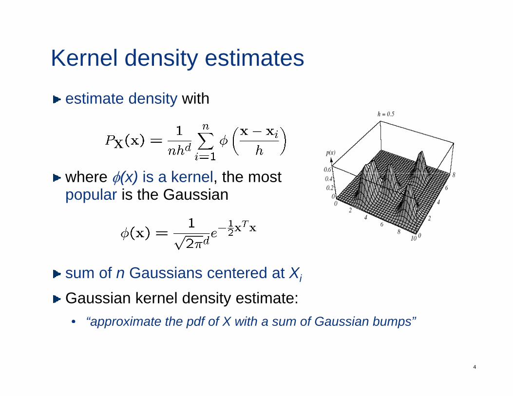
Kernel density estimatesestimate density with

h φ( ) i k l th twhere φ(x) is a kernel, the most popular is the Gaussian

sum of n Gaussians centered at Xsum of n Gaussians centered at Xi

Gaussian kernel density estimate:• “approximate the pdf of X with a sum of Gaussian bumps”

4

approximate the pdf of X with a sum of Gaussian bumps

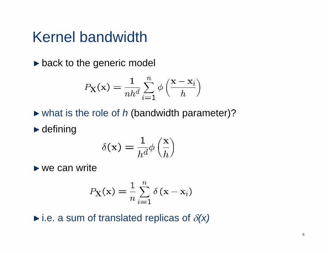
Kernel bandwidthback to the generic model

h t i th l f h (b d idth t )?what is the role of h (bandwidth parameter)?defining

we can write

5

i.e. a sum of translated replicas of δ(x)

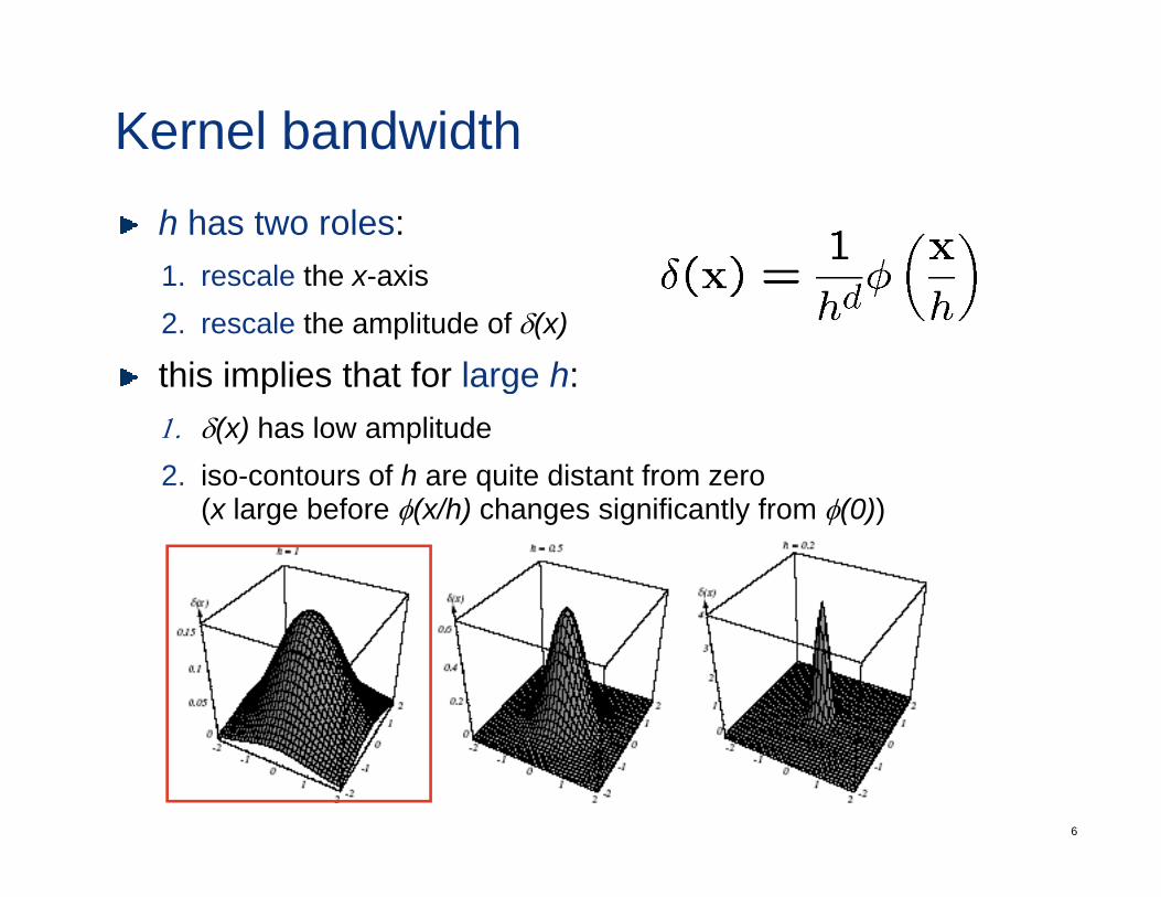
Kernel bandwidthh has two roles:1 rescale the x-axis1. rescale the x-axis2. rescale the amplitude of δ(x)

this implies that for large h:p g1. δ(x) has low amplitude2. iso-contours of h are quite distant from zero

(x large before φ(x/h) changes significantly from φ(0))(x large before φ(x/h) changes significantly from φ(0))

6

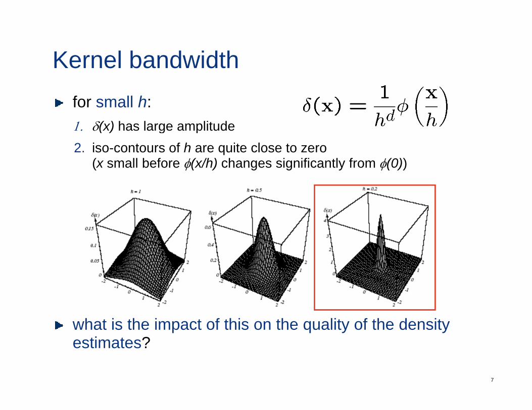
Kernel bandwidthfor small h:1 δ(x) has large amplitude1. δ(x) has large amplitude2. iso-contours of h are quite close to zero

(x small before φ(x/h) changes significantly from φ(0))

what is the impact of this on the quality of the density

7

estimates?

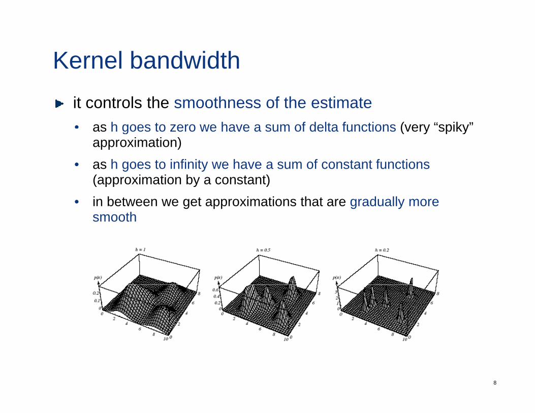
Kernel bandwidthit controls the smoothness of the estimate• as h goes to zero we have a sum of delta functions (very “spiky”as h goes to zero we have a sum of delta functions (very spiky

approximation)• as h goes to infinity we have a sum of constant functions

(approximation by a constant)(approximation by a constant)• in between we get approximations that are gradually more

smooth

8

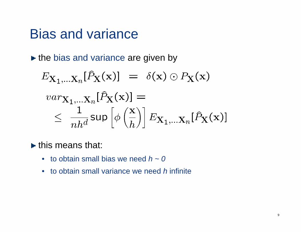
Bias and variancethe bias and variance are given by

this means that:• to obtain small bias we need h ~ 0to obtain small bias we need h 0• to obtain small variance we need h infinite

9

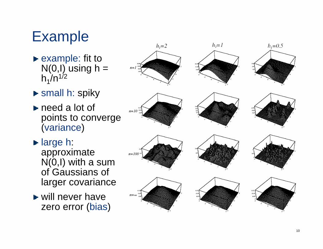
Exampleexample: fit to N(0,I) using h = h /n1/2h1/n1/2

small h: spikyneed a lot ofneed a lot of points to converge (variance)large hlarge h: approximateN(0,I) with a sum of Gaussians ofof Gaussians of larger covariancewill never have

(bi )

10

zero error (bias)

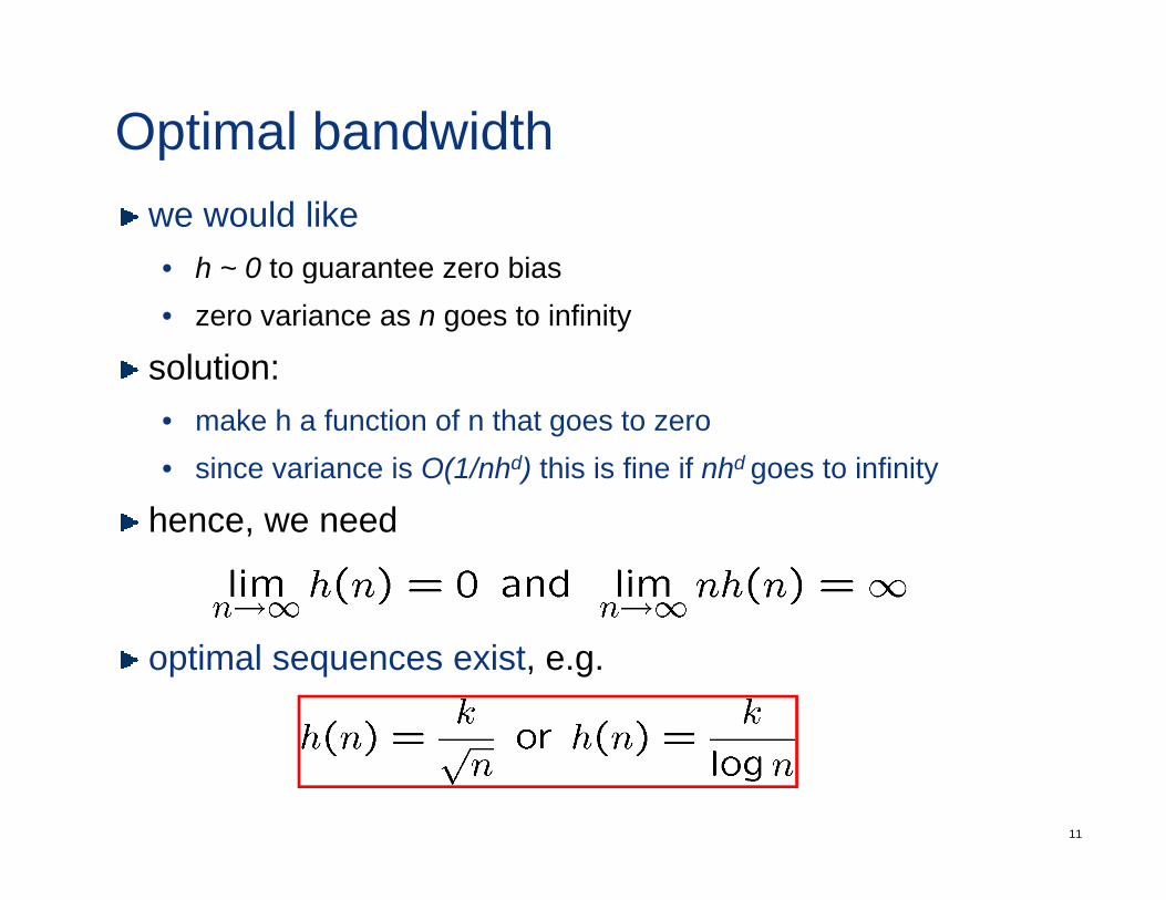
Optimal bandwidthwe would like• h ~ 0 to guarantee zero biasg• zero variance as n goes to infinity

solution:• make h a function of n that goes to zero• since variance is O(1/nhd) this is fine if nhd goes to infinity

h dhence, we need

optimal sequences exist, e.g.

11

Optimal bandwidthin practice this has limitations• does not say anything about the finite data case (the one we y y g (

care about)• still have to find the best k

ll d i t i l d t h iusually we end up using trial and error or techniques like cross-validation

12

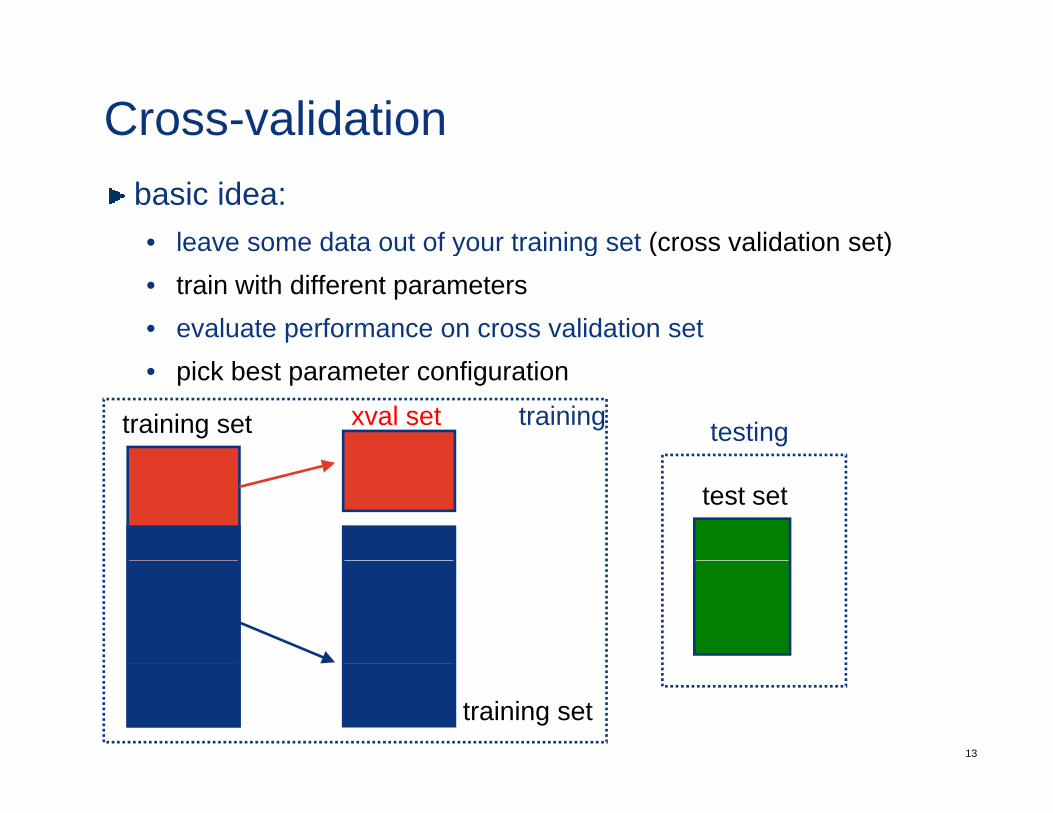
Cross-validationbasic idea:• leave some data out of your training set (cross validation set)y g ( )• train with different parameters• evaluate performance on cross validation set• pick best parameter configuration

training set xval set training testing

test set

13

training set

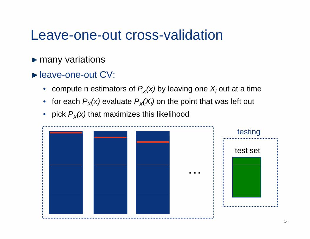
Leave-one-out cross-validationmany variationsleave one out CV:leave-one-out CV:• compute n estimators of PX(x) by leaving one Xi out at a time• for each PX(x) evaluate PX(Xi) on the point that was left outX( ) X( i) p• pick PX(x) that maximizes this likelihood

testing

test set

g

...

14

Non-parametric classifiersgiven kernel density estimates for all classes we can compute the BDRpsince the estimators are non-parametric the resulting classifier will also be non-parametricthis term is general and applies to any learning algorithma very simple example is the nearest neighbor classifier

15

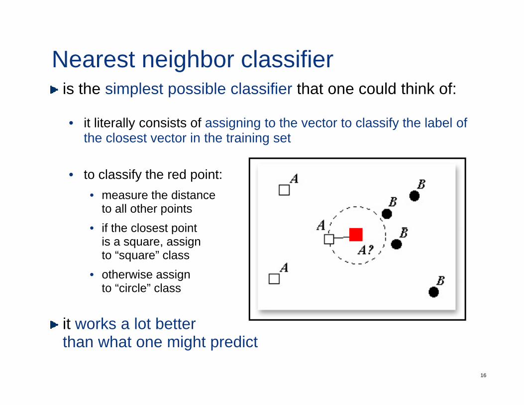
Nearest neighbor classifieris the simplest possible classifier that one could think of:

• it literally consists of assigning to the vector to classify the label ofit literally consists of assigning to the vector to classify the label of the closest vector in the training set

• to classify the red point:to classify the red point:• measure the distance

to all other points• if the closest point• if the closest point

is a square, assignto “square” class

• otherwise assigngto “circle” class

it works a lot better

16

than what one might predict

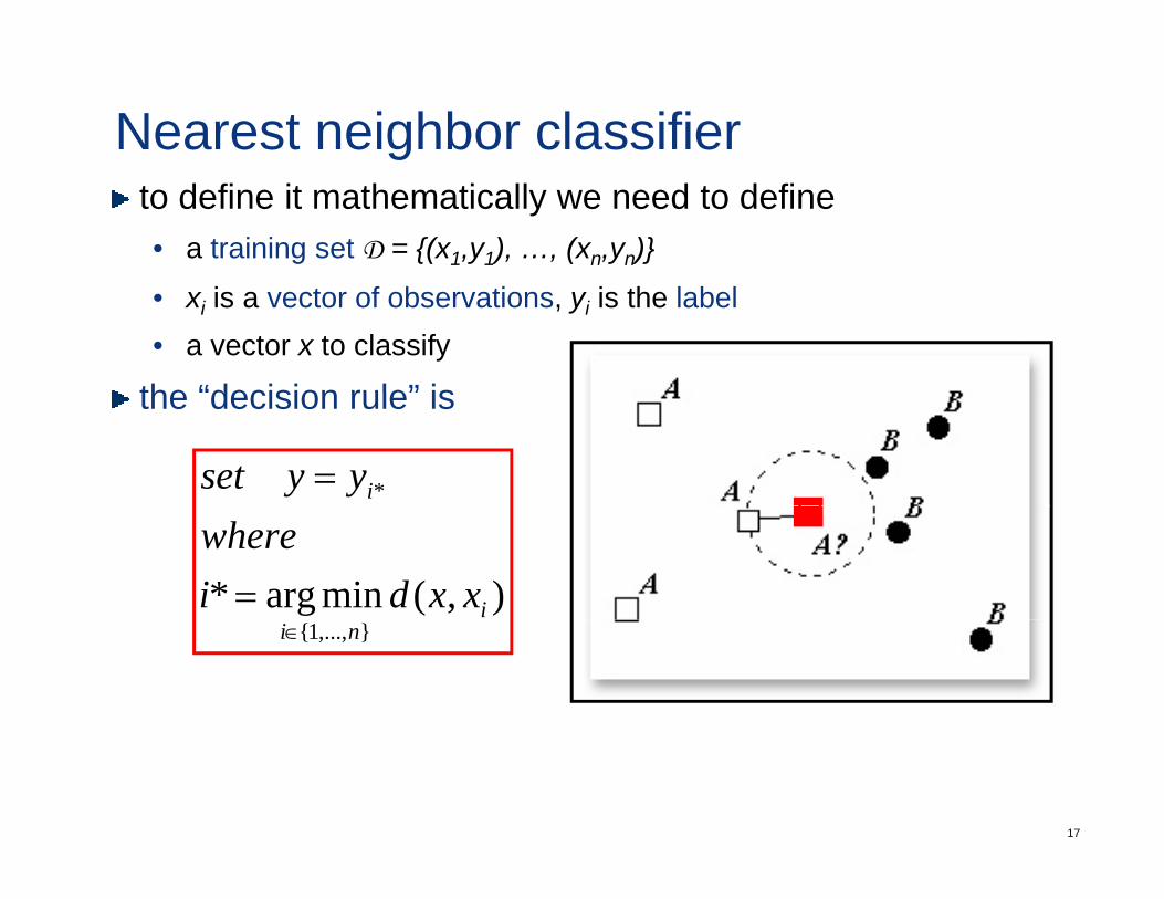
Nearest neighbor classifierto define it mathematically we need to define• a training set D = {(x1,y1), …, (xn,yn)}

• xi is a vector of observations, yi is the label• a vector x to classify

the “decision rule” isthe decision rule is

*iyyset =

),(minarg* ixxdiwhere

=},...,1{ ni∈

17

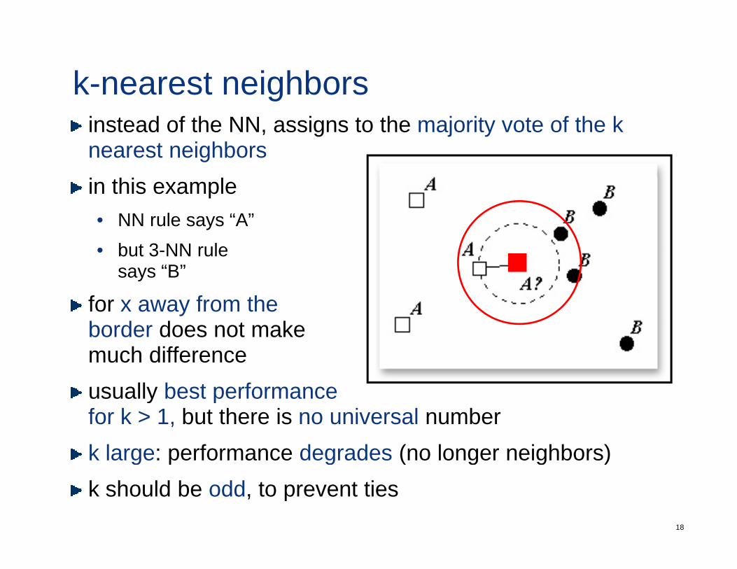
k-nearest neighborsinstead of the NN, assigns to the majority vote of the k nearest neighborsin this example• NN rule says “A”• but 3 NN rule• but 3-NN rule

says “B”

for x away from theborder does not makemuch differenceusually best performanceusually best performancefor k > 1, but there is no universal numberk large: performance degrades (no longer neighbors)

18

g p g ( g g )k should be odd, to prevent ties

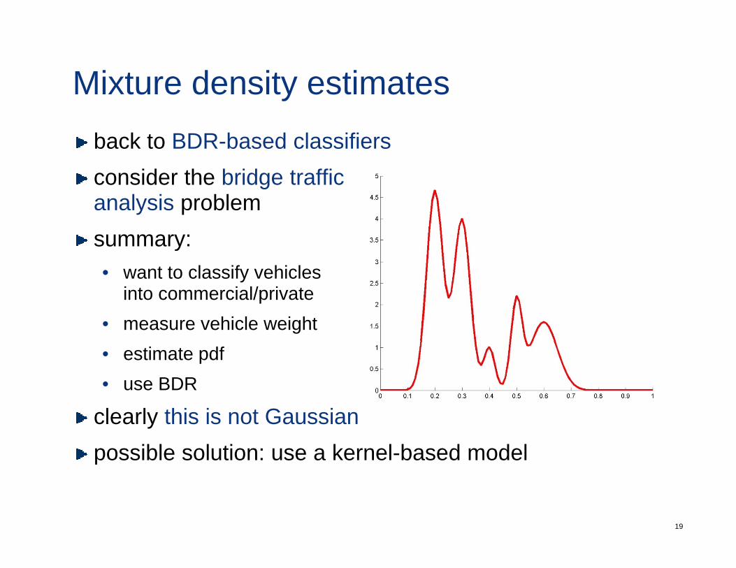
Mixture density estimatesback to BDR-based classifiersconsider the bridge trafficconsider the bridge traffic analysis problem summary:y• want to classify vehicles

into commercial/privatehi l i ht• measure vehicle weight

• estimate pdf• use BDR

clearly this is not Gaussianpossible solution: use a kernel-based model

19

p

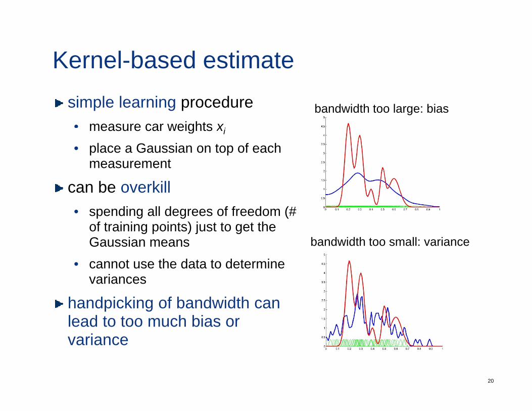
Kernel-based estimatesimple learning procedure• measure car weights xi

bandwidth too large: biasmeasure car weights xi

• place a Gaussian on top of each measurement

can be overkill• spending all degrees of freedom (#

of training points) just to get the g p ) j gGaussian means

• cannot use the data to determine variances

bandwidth too small: variance

variances

handpicking of bandwidth can lead to too much bias or

i

20

variance

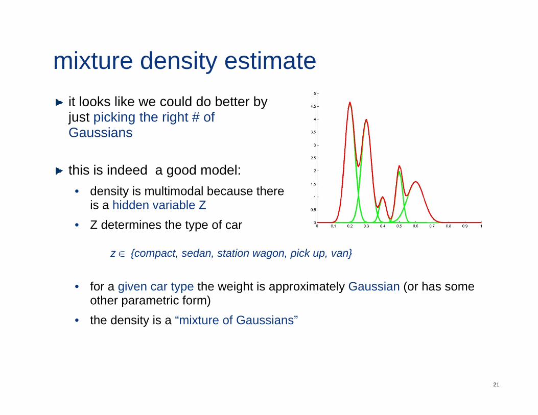
mixture density estimateit looks like we could do better byjust picking the right # of G iGaussians

this is indeed a good model:• density is multimodal because there

is a hidden variable Z• Z determines the type of car

z ∈ {compact, sedan, station wagon, pick up, van}

• for a given car type the weight is approximately Gaussian (or has some• for a given car type the weight is approximately Gaussian (or has some other parametric form)

• the density is a “mixture of Gaussians”

21

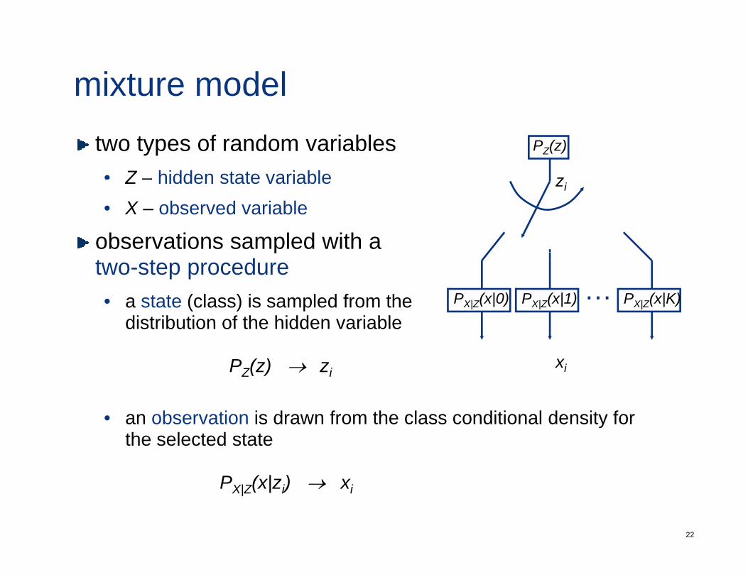
mixture modeltwo types of random variables• Z – hidden state variable

PZ(z)

zZ – hidden state variable• X – observed variable

observations sampled with a

zi

ptwo-step procedure• a state (class) is sampled from the

distribution of the hidden variablePX|Z(x|0) PX|Z(x|1) PX|Z(x|K)…

distribution of the hidden variable

PZ(z) → zixi

• an observation is drawn from the class conditional density for the selected state

22

PX|Z(x|zi) → xi

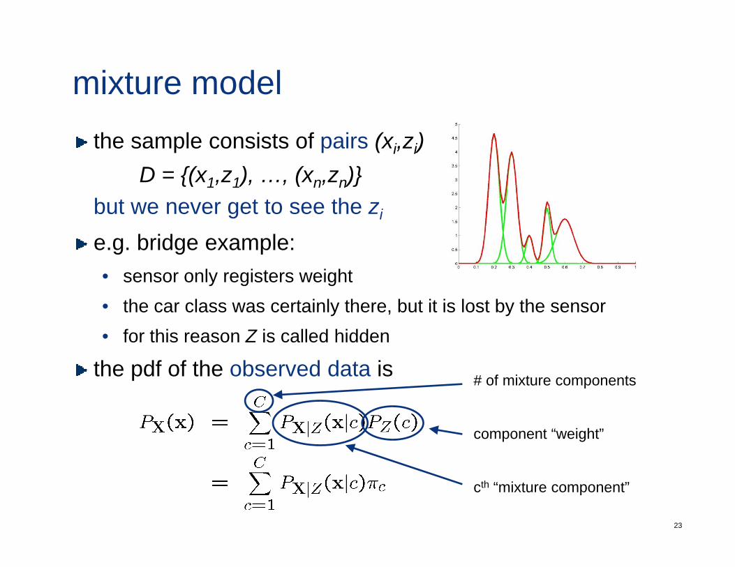
mixture modelthe sample consists of pairs (xi,zi)

D = {(x z ) (x z )}D = {(x1,z1), …, (xn,zn)}but we never get to see the zi

e.g. bridge example:e.g. bridge example:• sensor only registers weight• the car class was certainly there, but it is lost by the sensor• for this reason Z is called hidden

the pdf of the observed data is # of mixture components

component “weight”

23

cth “mixture component”

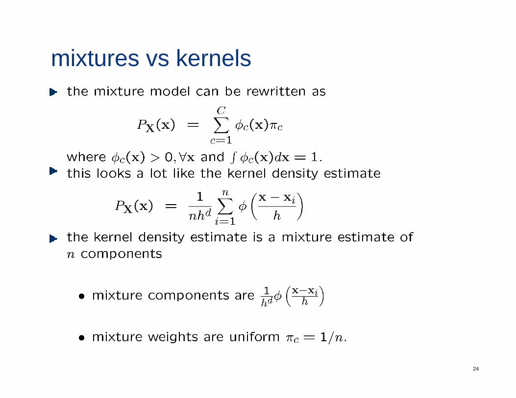
mixtures vs kernels

24

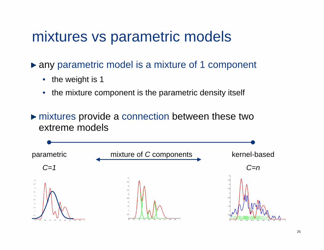
mixtures vs parametric models

any parametric model is a mixture of 1 componentthe eight is 1• the weight is 1

• the mixture component is the parametric density itself

mixtures provide a connection between these two extreme models

parametric

C=1

kernel-based

C=n

mixture of C components

25

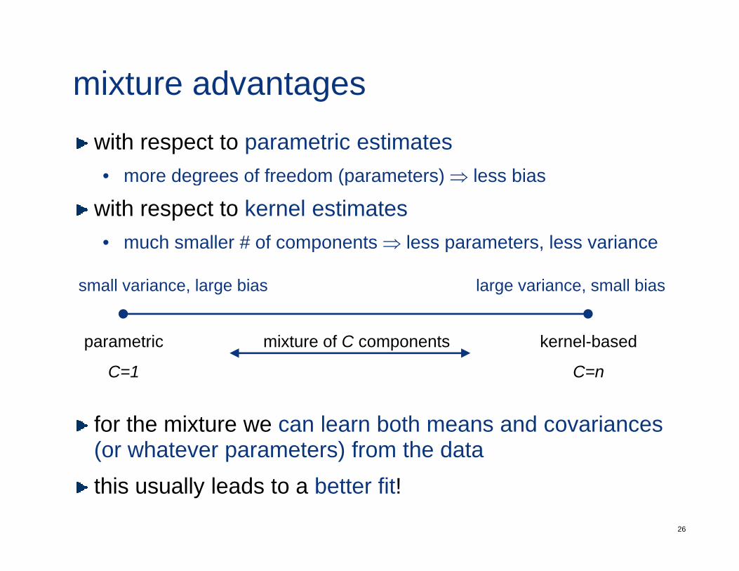
mixture advantageswith respect to parametric estimates• more degrees of freedom (parameters) ⇒ less bias• more degrees of freedom (parameters) ⇒ less bias

with respect to kernel estimates• much smaller # of components ⇒ less parameters, less variancep p ,

small variance, large bias large variance, small bias

parametric

C=1

kernel-based

C=n

mixture of C components

for the mixture we can learn both means and covariances (or whatever parameters) from the data

26

this usually leads to a better fit!

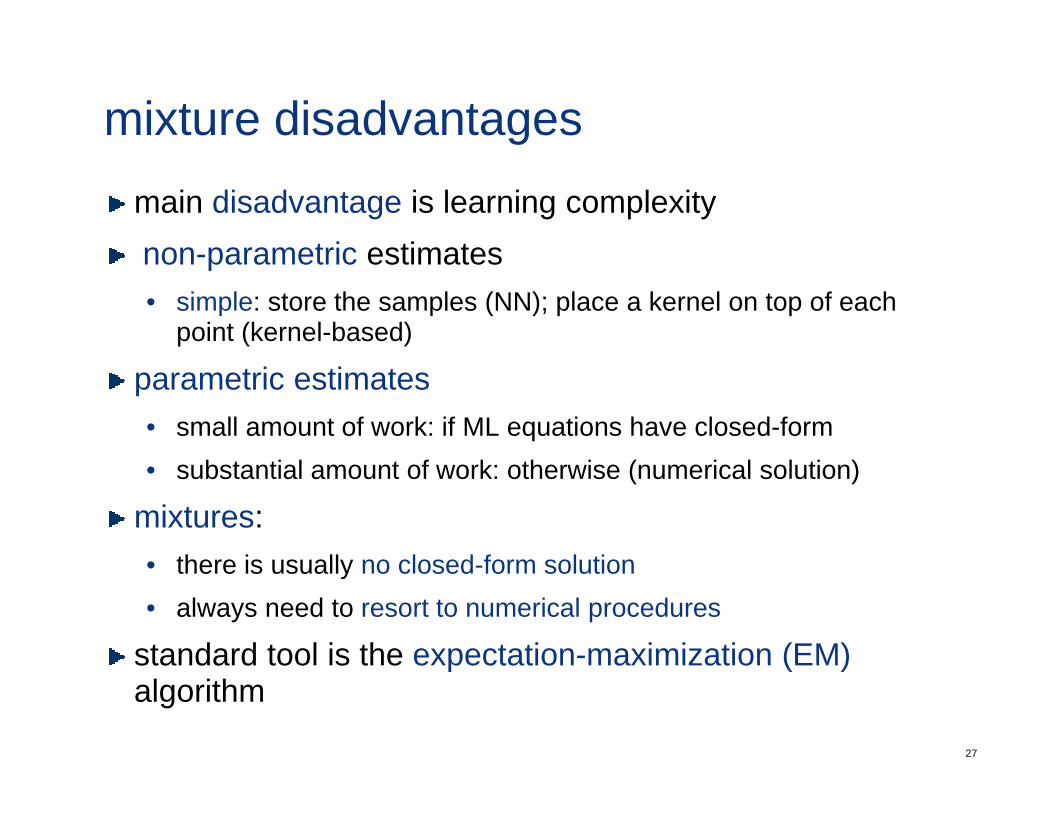
mixture disadvantagesmain disadvantage is learning complexitynon parametric estimatesnon-parametric estimates• simple: store the samples (NN); place a kernel on top of each

point (kernel-based)

parametric estimates• small amount of work: if ML equations have closed-form• substantial amount of work: otherwise (numerical solution)

mixtures:there is usually no closed form solution• there is usually no closed-form solution

• always need to resort to numerical procedures

standard tool is the expectation-maximization (EM)

27

standard tool is the expectation maximization (EM)algorithm

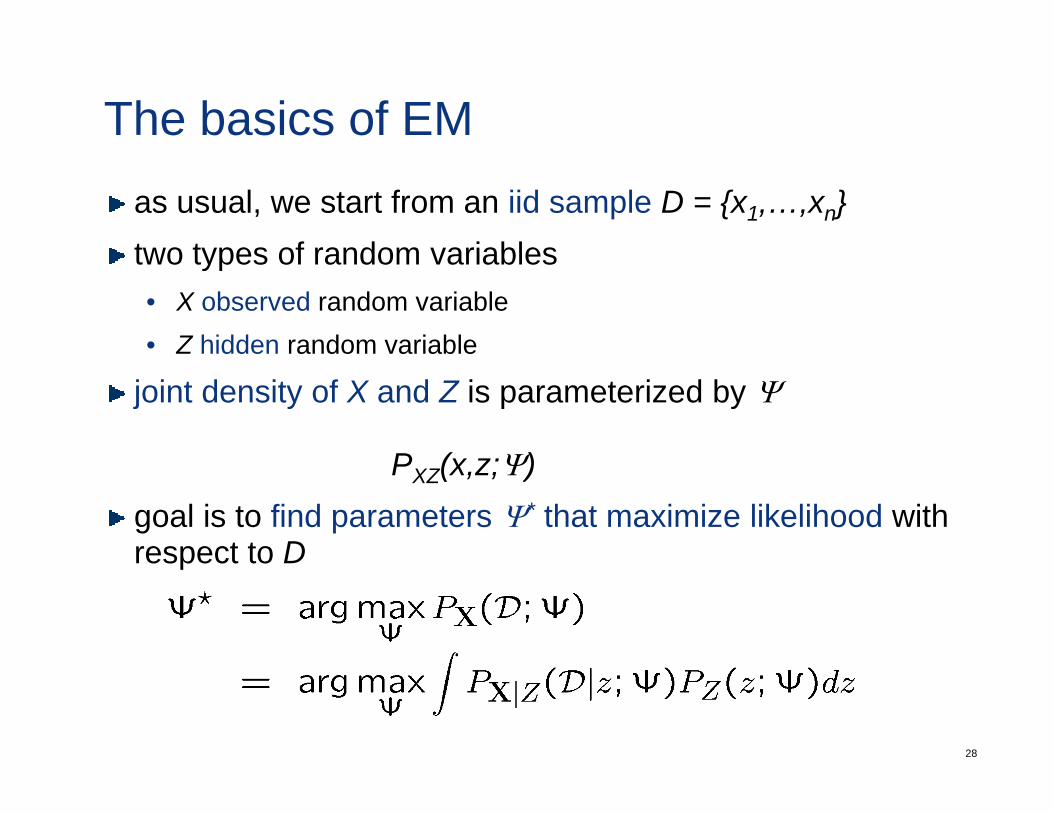
The basics of EMas usual, we start from an iid sample D = {x1,…,xn}two types of random variablestwo types of random variables• X observed random variable• Z hidden random variable

joint density of X and Z is parameterized by Ψ

P ( Ψ)PXZ(x,z;Ψ)goal is to find parameters Ψ* that maximize likelihood with respect to Drespect to D

28

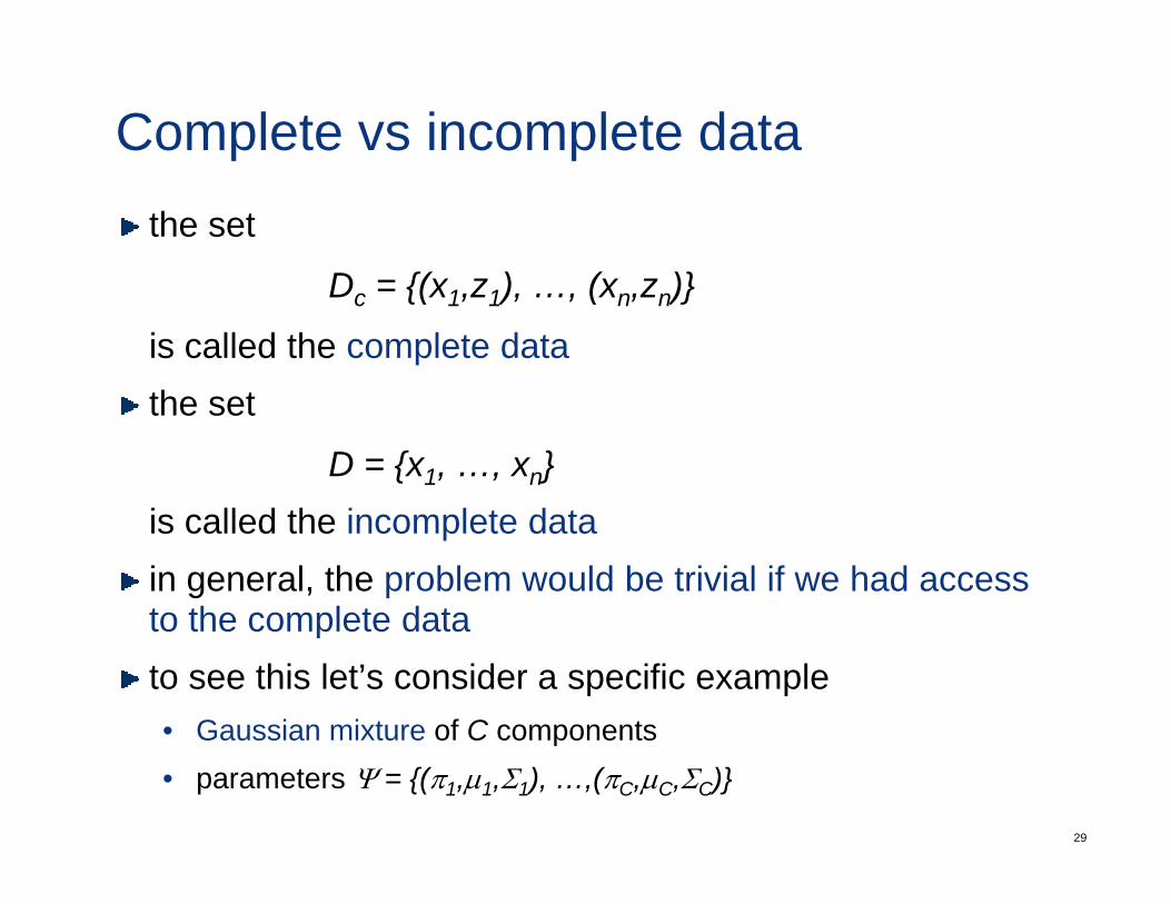
Complete vs incomplete datathe set

D = {(x z ) (x z )}Dc = {(x1,z1), …, (xn,zn)}

is called the complete datath tthe set

D = {x1, …, xn}i ll d th i l t d tis called the incomplete datain general, the problem would be trivial if we had access to the complete datato the complete datato see this let’s consider a specific example• Gaussian mixture of C components

29

Gaussian mixture of C components• parameters Ψ = {(π1,µ1,Σ1), …,(πC,µC,ΣC)}

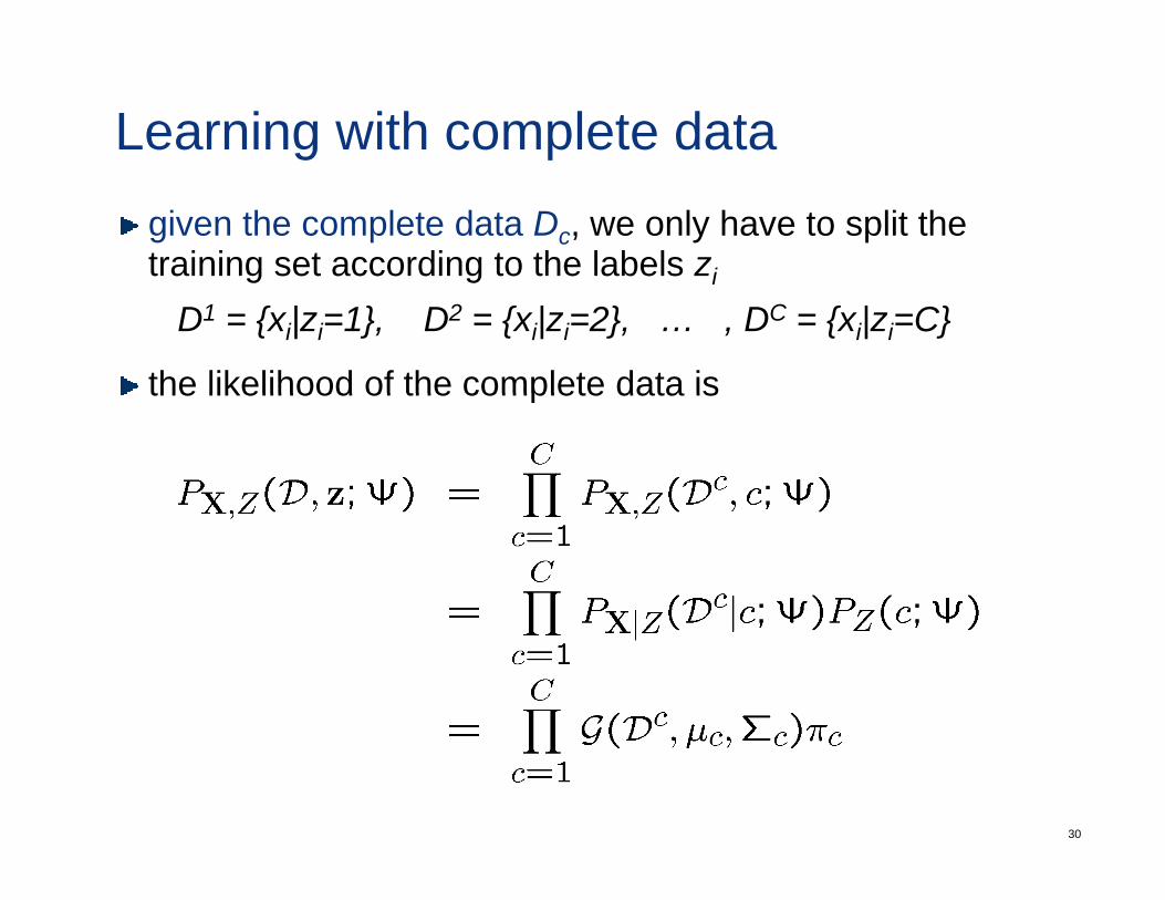
Learning with complete datagiven the complete data Dc, we only have to split the training set according to the labels zig g i

D1 = {xi|zi=1}, D2 = {xi|zi=2}, … , DC = {xi|zi=C}

the likelihood of the complete data isthe likelihood of the complete data is

30

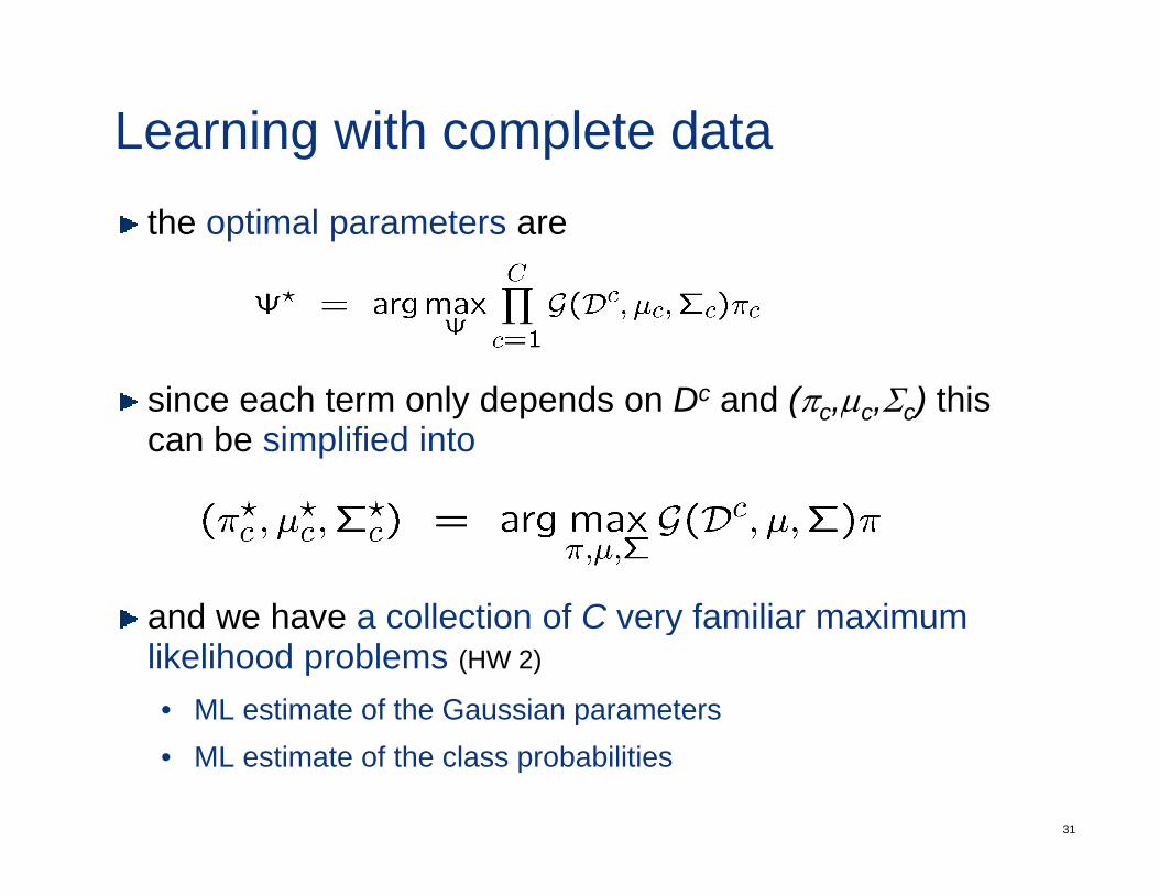
Learning with complete datathe optimal parameters are

i h t l d d Dc d ( Σ ) thisince each term only depends on Dc and (πc,µc,Σc) this can be simplified into

and we have a collection of C very familiar maximumand we have a collection of C very familiar maximum likelihood problems (HW 2)

• ML estimate of the Gaussian parameters

31

• ML estimate of the class probabilities

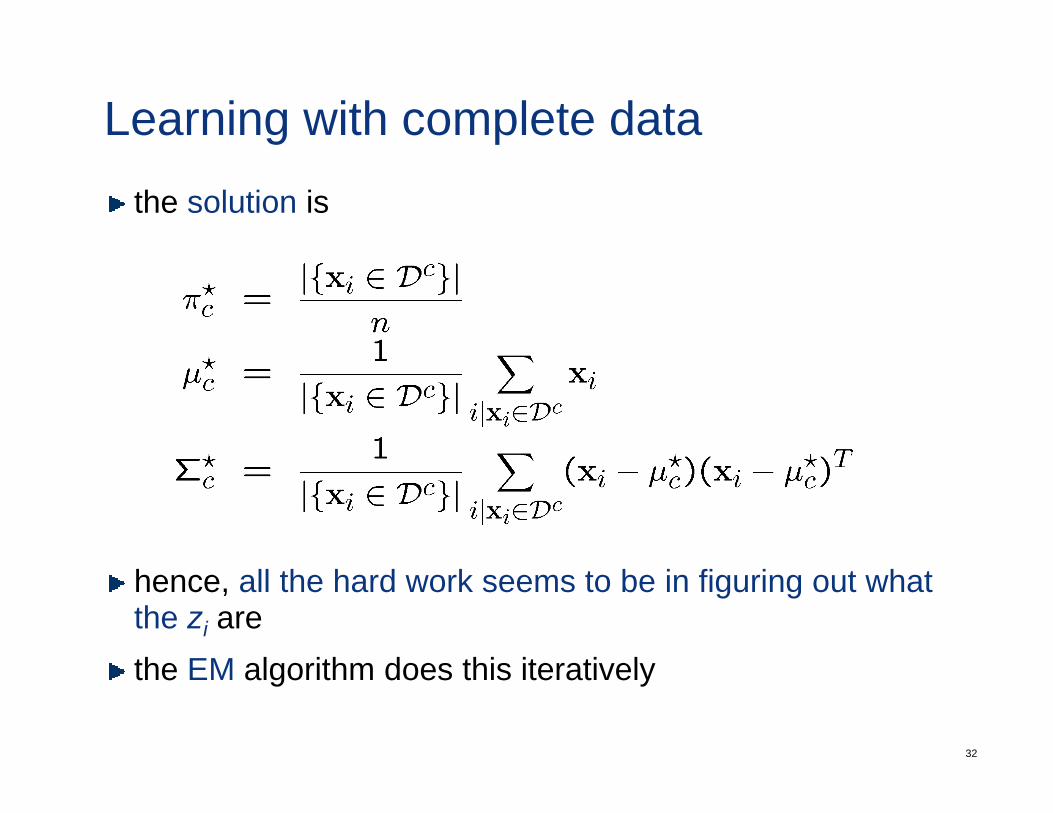
Learning with complete datathe solution is

hence, all the hard work seems to be in figuring out what the zi arethe EM algorithm does this iterati el

32

the EM algorithm does this iteratively

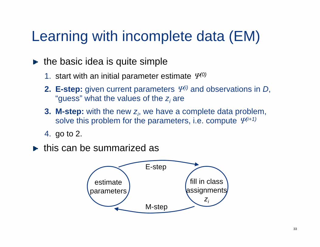
Learning with incomplete data (EM)the basic idea is quite simple1 start with an initial parameter estimate Ψ(0)1. start with an initial parameter estimate Ψ( )

2. E-step: given current parameters Ψ(i) and observations in D, “guess” what the values of the zi are

3. M-step: with the new zi, we have a complete data problem, solve this problem for the parameters, i.e. compute Ψ(i+1)

4. go to 2.

this can be summarized as

E-step

estimateparameters

fill in classassignments

zi

p

33

iM-step

47