mixed integer programming - co-at-work.zib.deco-at-work.zib.de/files/gurobi_mip.pdf · mixed...

Mixed Integer Programming

2 © 2015 Gurobi Optimization

Mixed Integer Programming

A mixed-integer program (MIP) is an optimization problem of the form

Why do we care about this problem?


Applications

Accounting

Advertising

Agriculture

Airlines

ATM provisioning

Compilers

Defense

Electrical power

Energy

Finance

Food service

Forestry

Gas distribution

Government

Internet applications

Logistics/supply chain

Medical

Mining

National research labs

Online dating

Portfolio management

Railways

Recycling

Revenue management

Semiconductor

Shipping

Social networking

Sports betting

Sports scheduling

Statistics

Steel Manufacturing

Telecommunications

Transportation

Utilities

Workforce scheduling

...


National Football League


NFL Schedule

NFL revenues (2014) from TVcontracts: ~$5 billion in 2014

256 games in regular season

Each team plays 16 games (with 1 BYE) over 17 weeks

Each team’s opponents are predetermined before scheduling

NFL begins scheduling immediately after Superbowl(once all opponents known)

Input from all 32 clubs (stadium blocks, travel considerations, competitive factors, etc.)

Input from all 5 television partners (key games, dates, markets, etc.)

Entire process takes 2-3 months


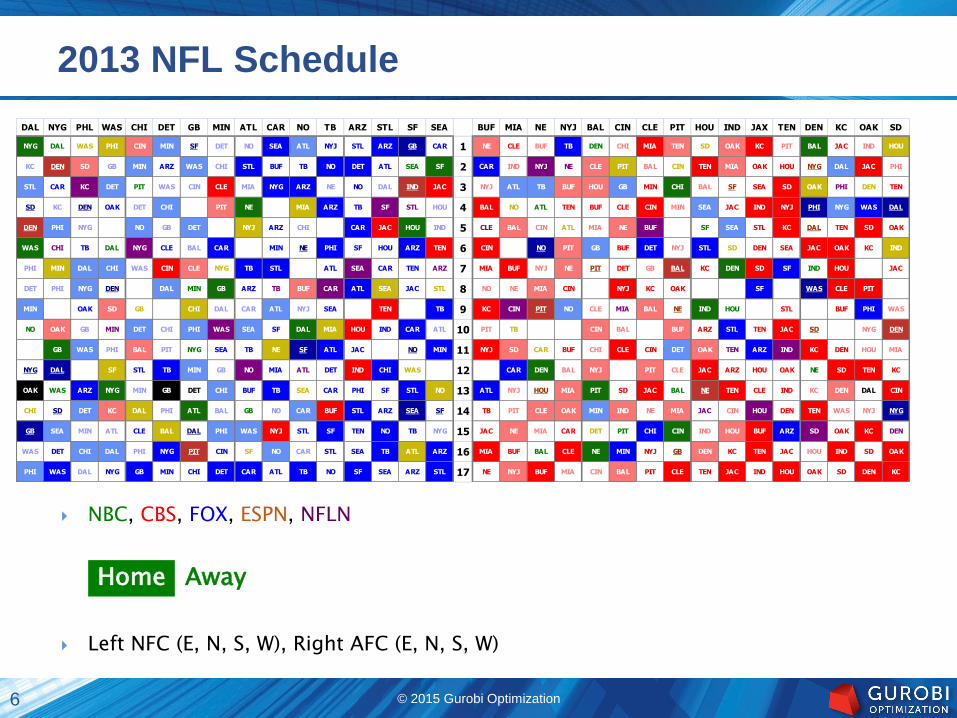
2013 NFL Schedule

NBC, CBS, FOX, ESPN, NFLN

Left NFC (E, N, S, W), Right AFC (E, N, S, W)

DAL NYG PHL WAS CHI DET GB MIN ATL CAR NO TB ARZ STL SF SEA BUF MIA NE NYJ BAL CIN CLE PIT HOU IND JAX TEN DEN KC OAK SD

NYG DAL WAS PHI CIN MIN SF DET NO SEA ATL NYJ STL ARZ GB CAR 1 NE CLE BUF TB DEN CHI MIA TEN SD OAK KC PIT BAL JAC IND HOU

KC DEN SD GB MIN ARZ WAS CHI STL BUF TB NO DET ATL SEA SF 2 CAR IND NYJ NE CLE PIT BAL CIN TEN MIA OAK HOU NYG DAL JAC PHI

STL CAR KC DET PIT WAS CIN CLE MIA NYG ARZ NE NO DAL IND JAC 3 NYJ ATL TB BUF HOU GB MIN CHI BAL SF SEA SD OAK PHI DEN TEN

SD KC DEN OAK DET CHI PIT NE MIA ARZ TB SF STL HOU 4 BAL NO ATL TEN BUF CLE CIN MIN SEA JAC IND NYJ PHI NYG WAS DAL

DEN PHI NYG NO GB DET NYJ ARZ CHI CAR JAC HOU IND 5 CLE BAL CIN ATL MIA NE BUF SF SEA STL KC DAL TEN SD OAK

WAS CHI TB DAL NYG CLE BAL CAR MIN NE PHI SF HOU ARZ TEN 6 CIN NO PIT GB BUF DET NYJ STL SD DEN SEA JAC OAK KC IND

PHI MIN DAL CHI WAS CIN CLE NYG TB STL ATL SEA CAR TEN ARZ 7 MIA BUF NYJ NE PIT DET GB BAL KC DEN SD SF IND HOU JAC

DET PHI NYG DEN DAL MIN GB ARZ TB BUF CAR ATL SEA JAC STL 8 NO NE MIA CIN NYJ KC OAK SF WAS CLE PIT

MIN OAK SD GB CHI DAL CAR ATL NYJ SEA TEN TB 9 KC CIN PIT NO CLE MIA BAL NE IND HOU STL BUF PHI WAS

NO OAK GB MIN DET CHI PHI WAS SEA SF DAL MIA HOU IND CAR ATL 10 PIT TB CIN BAL BUF ARZ STL TEN JAC SD NYG DEN

GB WAS PHI BAL PIT NYG SEA TB NE SF ATL JAC NO MIN 11 NYJ SD CAR BUF CHI CLE CIN DET OAK TEN ARZ IND KC DEN HOU MIA

NYG DAL SF STL TB MIN GB NO MIA ATL DET IND CHI WAS 12 CAR DEN BAL NYJ PIT CLE JAC ARZ HOU OAK NE SD TEN KC

OAK WAS ARZ NYG MIN GB DET CHI BUF TB SEA CAR PHI SF STL NO 13 ATL NYJ HOU MIA PIT SD JAC BAL NE TEN CLE IND KC DEN DAL CIN

CHI SD DET KC DAL PHI ATL BAL GB NO CAR BUF STL ARZ SEA SF 14 TB PIT CLE OAK MIN IND NE MIA JAC CIN HOU DEN TEN WAS NYJ NYG

GB SEA MIN ATL CLE BAL DAL PHI WAS NYJ STL SF TEN NO TB NYG 15 JAC NE MIA CAR DET PIT CHI CIN IND HOU BUF ARZ SD OAK KC DEN

WAS DET CHI DAL PHI NYG PIT CIN SF NO CAR STL SEA TB ATL ARZ 16 MIA BUF BAL CLE NE MIN NYJ GB DEN KC TEN JAC HOU IND SD OAK

PHI WAS DAL NYG GB MIN CHI DET CAR ATL TB NO SF SEA ARZ STL 17 NE NYJ BUF MIA CIN BAL PIT CLE TEN JAC IND HOU OAK SD DEN KC

Home Away


Partial list of rules and goals

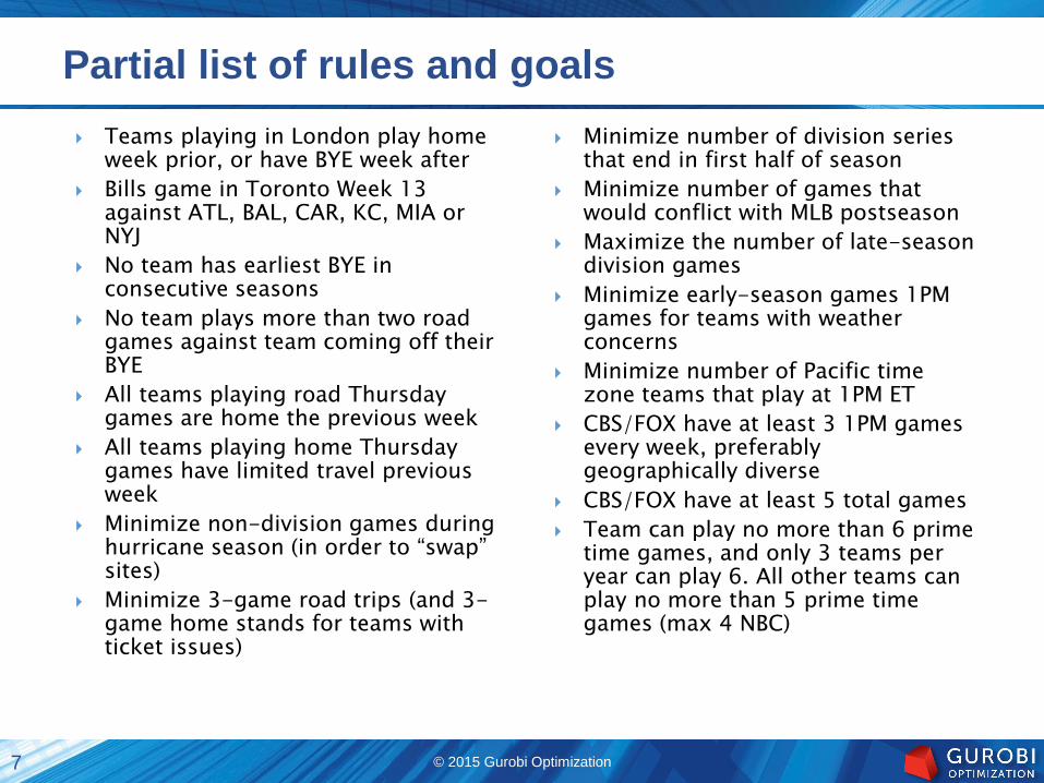
Teams playing in London play home week prior, or have BYE week after

Bills game in Toronto Week 13 against ATL, BAL, CAR, KC, MIA or NYJ

No team has earliest BYE in consecutive seasons

No team plays more than two road games against team coming off their BYE

All teams playing road Thursday games are home the previous week

All teams playing home Thursday games have limited travel previous week

Minimize non-division games during hurricane season (in order to “swap” sites)

Minimize 3-game road trips (and 3-game home stands for teams with ticket issues)

Minimize number of division series that end in first half of season

Minimize number of games that would conflict with MLB postseason

Maximize the number of late-season division games

Minimize early-season games 1PM games for teams with weather concerns

Minimize number of Pacific time zone teams that play at 1PM ET

CBS/FOX have at least 3 1PM games every week, preferably geographically diverse

CBS/FOX have at least 5 total games

Team can play no more than 6 prime time games, and only 3 teams per year can play 6. All other teams can play no more than 5 prime time games (max 4 NBC)


DAL NYG PHL WAS CHI DET GB MIN ATL CAR NO TB ARZ STL SF SEA BUF MIA NE NYJ BAL CIN CLE PIT HOU IND JAX TEN DEN KC OAK SD

BB

MON

BB

SUN

BB

SU-MO 1BB

SU-MO

BB

SU-MO

BB

SUN

BB

SUN

BB

SUN

BB

SUN

BB

MON

COLL.

FB

BB

SU-MOLEASE 2

BB

THU

BB

TH-MOLEASE

BB

MON

BB

MON

BB

MON

BB

SUN

BB

TH-SUHOME

PGA

TOURLEASE

BB

MON 3BB

MON

COLL.

FB

HOME

SNFNO THU

BB

SUN

BB

TH-SU

BB

SU-MO

BB

TH-SU

BON

JOVILONDON

BB

SUN 4BON

JOVI

BB

TH-SU

BB

SUNLONDON

BB

THU*

DIV DIV DIV BYE NO THU 5 DIV DIV BYE LEASE NASCAR DIV DIV

LCS LCS Marathon NASCAR LEASE AUTO 6 CARNIVAL LCS LCS LCS

LCS LCS NO THU AWAY 7 LCS LCS LCS

WS WS Marathon LONDON MLS 8 WS WS LONDON WS

NO THU BYE 9 BYE

LEASE MLS? 10 LEASE

SOCCER NO THU LEASE 11 NO MNFNO

PRIME

MLS? 12 LEASE NO MNF

TGIV TGIVNO

SUN 1p 13HIGH

SCHOOL

KU

HOOPSSEC ACC

NO

SUN 1pLEASE

MLS

CUP 14 Toronto? LEASE BIG 10

ARMY

NAVYNO SUN LEASE? 15

16

BELK 17

Stadium blocks

Of the 544 potential sites, almost 20% unavailable or had some sort of conflict

13 teams had 4 or more potential conflicts, affecting 25% or more of their potential home dates


A $5 billion MIP Model?

All constraints captured in one MIP:

◦ original: 25K rows, 20K cols, 800K nz

◦ presolved: 6K rows, 6K cols, 160K nz

3600 binary variables

What does a solution look like:

◦ 256 binary variables to set to 1

Each captures the particulars of one game

◦ the rest set to 0


New York Independent System Operator


What is NYISO?

NYISO is a non-profit,statutory agency

◦ began operating in 1999

NYISO primary responsibilities:

◦ operating New York's high-voltage grid

◦ administering and monitoring state's wholesale electricity markets

◦ long-term planning for high-voltage grid

reliability, future maintenance and expansion

Size

◦ grid encompasses 11,000 miles of transmission lines

◦ manages 500 power-generation units

◦ administers $7.5 billion in annual transactions


Optimization Plays a Central Role In NYISO Operations

Day-ahead problem

◦ unit-commitment for the next day: which units to be used

markets close 5 am

commitments must be posted by 11 am

30 minutes available to compute commitments

Real-time problem

◦ solved every 5 minutes, restricted unit-commitment

Real-time dispatch (EASY!)

◦ linear program, solved every 5 minutes

◦ determines generator clearing prices


Traditional Solution Approach: Lagrangian Relaxation (LR)

In use since the early 1980s

Claimed to produce high-quality solutions

Solution times are quite good

Considerable reluctance to make a change

However in 1999 MIP was demonstrated to be a viable alternative*

◦ pressure was mounting to switch

*Rutgers academic-industry meeting sponsored by Federal Energy Regulatory Commission (FERC).


Experience in Other ISOs*

In 2004, PJM implemented MIP in its day-ahead market

◦ estimated of annual production cost savings of $60 million

In 2006, PJM implemented MIP in its real-time market look-ahead

◦ test findings of $100 million in annual savings

In April 2009, CAISO implemented MIP as part of its Market Redesign and Technology Update

◦ estimated savings of $52 million

In 2009, the Southwest Power Pool (SPP) introduced MIP enhancements to its day-ahead market

◦ estimated $103 million in annual benefits

*FERC Staff Report, 2011 (Recent ISO Software Enhancements and Future Software and Modeling Plans)


MIP: Other Advantages

Maintainability

◦ LR code: 100,000 lines of FORTRAN

◦ understood by only one or two people

Transparency

◦ MIP formulation has much simpler representation

easy to read, interpret, and maintain

◦ solutions much easier to defend against legal challenges

Extensibility

◦ extremely difficult to add constraints to LR

◦ new constraints easy to add to MIP formulation

combined cycle-generator modeling enabled


Solution Implementation

Solution launch date: Q2 2014

Computing environment

◦ 50 HPUX client machines

◦ 12 Linux compute servers (3-production, 3-stage, 3-development)

Estimated savings: $4M yearly production costs

Future

◦ underlying models are highly nonlinear

MIP speed improvements can always be used to improve model accuracy

◦ conclusion:

continued MIP improvements will lead directly to efficiency gains in electrical-power markets!


Conclusion: Use MIP Instead of Custom Solution!

Easier to maintain a MIP model than complex source code

Easier to extend a MIP model than to adapt a custom algorithm

Easier to demonstrate correctness of a MIP model

Benefit from performance improvements over time coming from MIP solver vendors

◦ algorithmic speed-up exceeded hardware speed-up during the last 20 years!


Solving Mixed Integer Programs


MIP Application Types

Static MIP

◦ Formulate problem

◦ Solve it with a black-box MIP algorithm

◦ Read solution

◦ Potentially adjust problem and iterate

◦ most frequent use of MIP in practical applications

Branch-and-cut

◦ Problem has too many constraints to formulate in static fashion

e.g., classical TSP model: exponentially many sub-tour elimination constraints

◦ Construct partial problem

◦ Add violated constraints on demand

"Lazy constraint" separation callback: cut off primal infeasible LP or IP solutions

Branch-and-price

◦ Problem has too many variables to formulate in static fashion

e.g., many public transport and airline problems are solved via B&P

◦ Pricing callback: cut off dual infeasible LP solutions

◦ Usually needs problem specific branching rule that is compatible with pricing

◦ Heuristic variant: column generation

Only apply pricing for the root LP, then solve static MIP with resulting set of variables


MIP Building Blocks

Presolve

◦ Tighten formulation and reduce problem size

Solve continuous relaxations

◦ Ignoring integrality

◦ Gives a bound on the optimal integral objective

Cutting planes

◦ Cut off relaxation solutions

Branching variable selection

◦ Crucial for limiting search tree size

Primal heuristics

◦ Find integer feasible solutions


MIP Building Blocks

Presolve





Cutting planes




Primal heuristics



LP Presolve

Goal

◦ Reduce the problem size

Speedup linear algebra during the solution process

Example

x + y + z ≤ 5 (1)u – x – z = 0 (2)………0 ≤ x, y, z ≤ 1 (3)u is free (4)

Reductions

◦ Redundant constraint

(3) x + y + z ≤ 3, so (1) is redundant

◦ Substitution

(2) and (4) u can be substituted with x + z


MIP Presolve

Goals:

◦ Reduce problem size

Speed-up linear algebra during the solution process

◦ Strengthen LP relaxation

◦ Identify problem sub-structures

Cliques, implied bounds, networks, disconnected components, ...

Similar to LP presolve, but more powerful:

◦ Exploit integrality

Round fractional bounds and right hand sides

Lifting/coefficient strengthening

Probing

◦ Does not need to preserve duality

We only need to be able to uncrush a primal solution

Neither a dual solution nor a basis needs to be uncrushed


MIP Presolve

Goals:

◦ Reduce problem size

Speed-up linear algebra during the solution process

◦ Strengthen LP relaxation

◦ Identify problem sub-structures

Cliques, implied bounds, networks, disconnected components, ...

Similar to LP presolve, but more powerful:

◦ Exploit integrality

Round fractional bounds and right hand sides

Lifting/coefficient strengthening

Probing

◦ Does not need to preserve duality

We only need to be able to uncrush a primal solution

Neither a dual solution nor a basis needs to be uncrushed

modelwithout presolve with presolve

rows cols LP obj rows cols LP obj

roll3000 2291 1166 11097.1 987 855 11120.0

neos-787933 1897 236376 3.0 41 126 30.0


Single-Row Reductions

Clean-up rows

◦ Discard empty rows

◦ Discard redundant inequalities: sup{Ar⋅x} ≤ br

◦ Remove coefficients with tiny impact |aij⋅(uj-lj)|

Bound strengthening

◦ arj > 0, s:= br - inf{Ar⋅x} xj ≤ lj + s/arj

◦ arj < 0, s:= br - inf{Ar⋅x} xj ≥ uj + s/arj

Coefficient strengthening for inequalities

◦ j ∈ I, arj > 0, t:= br - sup{Ar⋅x} + arj > 0

arj := arj – t, br := br - ujt

2x – y ≤ 1

x – y ≤ 0

s/arj


Single-Row Reductions – Performance

0

0.1

0.2

0.3

0.4

0.5

0.6

0.7

0.8

39%

70%

24%

14%

27%

22%

1%

79%

74%

51%

60%

52%

44%

1%

6.4

%

4.8

%

3.3

%

5.7

%

4.6

%

0.0

%

0.9

%

affected (orig) affected (all) performance impact

benchmark data based on Gurobi 5.6

Key to these performance slides:

◦ affected (orig):

Disabled all presolve methods except for one particular reduction, abort after initial presolve

Chart shows fraction of models for which this method found a reduction in the presolve of the original model

◦ affected (all):

Disabled this one particular reduction, compare vs. default run with all reductions enabled

Chart shows number of models where disabling the reduction changes solution path

◦ performance impact

Disabled this one particular reduction, compare vs. default run with all reductions enabled

Chart shows performance degradation due to disabling the reduction

◦ top right number ("23%")

performance degradation from disabling all presolvereductions on this slide


Single-Row Reductions – Performance

0

0.1

0.2

0.3

0.4

0.5

0.6

0.7

0.8

39%

70%

24%

14%

27%

22%

1%

79%

74%

51%

60%

52%

44%

1%

6.4

%

4.8

%

3.3

%

5.7

%

4.6

%

0.0

%

0.9

%




Single-Column Reductions

Remove fixed variables and empty columns

◦ If |uj-lj| ≤∊, fix to some value in [lj,uj] and move terms to rhs

◦ Choice of value can be very tricky for numerical reasons

Round bounds of integer variables

Strengthen semi-continuous and semi-integer variables

Dual fixing, substitution, and bound strengthening

◦ Variable xj does not appear in equations

◦ cj ≥ 0, A⋅j ≥ 0 xj := lj

◦ cj ≥ 0, A⋅j ≥ 0 except for aij < 0,

z = 0 → row i redundant, xj := lj + (uj-lj)⋅zz = 1 → xj = uj

◦ cj ≥ 0, all rows i with aij < 0 redundant for xj ≥ t xj ≤ max{lj,t}


Single-Column Reductions – Performance

0

0.1

0.2

0.3

0.4

0.5

0.6

0.7

0.8

FIXED VARS SEMI-CONT/INT DUAL

STRENGTHENING

COMPL. SLACK AGGREGATE

25%

0%

41%

37%

57%

65%

0%

64%

61%

77%

2.7

%

0.5

% 7.0

%

3.1

%

29.8

%




Multi-Row Reductions

Parallel rows

◦ Search for pairs of rows such that coefficient vectors are parallel to each other

◦ Discard the dominated row, or merge two inequalities into an equation

Sparsify

◦ Add equations to other rows in order to cancel non-zeros

◦ Can also add inequalities with explicit slack variables

Multi-row bound and coefficient strengthening

◦ Like single-row version, but use other rows to get tighter bound on infimum and supremum tighter bounds, better coefficients

Clique merging

◦ Merge multiple cliques into larger single clique, e.g.:

x1 + x2 ≤ 1x1 + x3 ≤ 1

x2 + x3 ≤ 1

with binary variables x1, x2, x3 can be merged into

x1 + x2 + x3 ≤ 1


Multi-Row Reductions

0

0.1

0.2

0.3

0.4

0.5

0.6

0.7

0.8

PARALLEL ROWS SPARSIFY BOUND/COEFF STR. CLIQUE MERGING

37%

34%

65%

16%

63%

55%

76%

55%

1.7

% 6.3

%

17.9

%

16.1

%




Multi-Column Reductions

Fix redundant penalty variables

◦ Penalty variables: support(A⋅j) = 1

◦ Multiple penalty variables in a single constraint

Some can be fixed if others can accomplish all that is needed

Parallel columns (say, columns 1 and 2): A⋅1 = sA⋅2

◦ u2 = ∞, c1 ≥ sc2, 2 ∉ I or (|s| = 1, {1,2} ⊆ I): x1 := l1

◦ l2 = -∞, c1 ≤ sc2, 2 ∉ I or (|s| = 1, {1,2} ⊆ I): x1 := u1

◦ c1 = sc2, 1,2 ∉ I or (|s| = 1, {1,2} ⊆ I): x1' := x1 + sx2

◦ Detection algorithm: two level hashing plus sorting

Dominated columns: A⋅1 ≥ sA⋅2, only inequalities

◦ u2 = ∞, c1 ≥ sc2, 2 ∉ I or (|s| = 1, {1,2} ⊆ I): x1 := l1

◦ Detection algorithm: essentially pair-wise comparison

Can be very expensive: needs work limit


Multi-Column Reductions – Performance

0

0.1

0.2

0.3

0.4

0.5

0.6

PENALTY VARS PARALLEL COLS DOMINATED COLS

5%

31%

29%

9%

59%

57%

0.0

%

5.7

%

5.0

%




Full Problem Reductions

Symmetric variable substitution

◦ Integer variables in same orbit can be aggregated if the involved symmetries do not overlap

◦ Continuous variables in same orbit can always be aggregated

◦ Issue: symmetry detection can sometimes be time consuming!

Probing

◦ Tentatively fix binary x = 0 and x = 1, propagate fixing to get domain reductions for other variables

x = 0 → y ≤ u0, x = 1 → y ≤ u1 y ≤ max{u0,u1} (bound strength.)

x = 0 → y = ly, x = 1 → y = uy y := ly + (uy-ly)⋅x (substitution)

ay ≤ b, x = 1 → ay ≤ d < b ay + (b-d)⋅x ≤ b (lifting)

◦ Sequence dependent

◦ Can be very time consuming

Needs specialized data structures and algorithms

Implied Integer Detection

◦ Primal version: ax + y = b, x integer variables, a ∈ ℤn, b ∈ ℤ y integer

◦ Dual version:

One of the inequalities for y will be tight, but do not know which

If all those inequalities lead to primal version of implied integer detection, y is implied integer


Full Problem Reductions

0

0.1

0.2

0.3

0.4

0.5

0.6

0.7

0.8

SYMM VARS PROBING IMPLIED INT

29%

78%

45%

4%

70%

67%

4.6

%

15.5

% 21.6

%




MIP Building Blocks

Presolve





Cutting planes




Primal heuristics



Primal and Dual LP

Primal Linear Program:

Weighted combination of constraints (y) and bounds (z) yields

Dual Linear Program:

0

..

min

x

bAxts

xcT

0

..

max

z

czAyts

byTTT

T

0 with zbyxzAxy TTT

Strong Duality Theorem:

(if primal and dual are both feasible)

byxcTT


Karush-Kuhn-Tucker Conditions

Conditions for LP optimality:

◦ Primal feasibility: Ax = b (x ≥ 0)

◦ Dual feasibility: ATy + z = c (z ≥ 0)

◦ Complementarity: xTz = 0

Primal feas Dual feas ComplementarityPrimal simplex Maintain Goal MaintainDual simplex Goal Maintain MaintainBarrier Goal Goal Goal


Simplex Algorithm

Phase 1: find some feasible vertex solution

objective


Simplex Algorithm

Pricing: find directions in which objective improves and select one of them

◦ Gurobi parameters: SimplexPricing, NormAdjust

objective


Simplex Algorithm

Ratio test: follow outgoing ray until next vertex is reached

objective


Simplex Algorithm

Iterate until no more improving direction is found

objective


MIP – LP Relaxation

objective

MIP-optimal solutions

LP-optimal solutions


No feasible solutions can be better than an LP optimum

MIP – LP Relaxation

objective

MIP-optimal solutions

LP-optimal solutions


Side Note – Performance Variability

Measuring performance of MIP is a difficult task

Seemingly performance neutral changes can have a dramatic impact on the solve time for an individual model

◦ Changing the random seed

◦ Permuting the columns and rows

e.g., store model in *.lp file format and reading it back in

◦ Solving model on a different machine

Different operating system

Different CPU

Main reason: degeneracy of LP relaxation

◦ Most models have multiple optimal solutions to their LP relaxation

◦ LP solver's choice of solution is arbitrary

Depends on random seed, column and row ordering, tiny differences in numerics

◦ Different optimal solution vector leads to different cutting planes, different branching decisions, and thus different search tree

Conclusion: need big test set to measure performance

◦ Use multiple random seeds to artificially increase test set

More on performance variability: tomorrow


MIP Building Blocks

Presolve





Cutting planes




Primal heuristics



fractional LP-optimal solution

MIP – Cutting Planes

objective




objective




objective

new LP-optimal solution



objective


No feasible solutions can be better than an LP optimum


objective

improved dual bound


Cutting Planes – Overview

General-purpose cutting planes

◦ Gomory mixed integer cuts

◦ Mixed Integer Rounding (MIR) cuts

◦ Flow cover cuts

◦ Lift-and-project (L&P) cuts

◦ Zero-half and mod-k cuts

◦ ...

Structural cuts

◦ Implied bound cuts

◦ Knapsack cover cuts

◦ GUB cover cuts

◦ Clique cuts

◦ Multi-commodity-flow (MCF) cuts

◦ Flow path cuts

◦ ...


Chvatal-Gomory Cuts

Consider a rational polyhedron

P = {x ∈ Rn | Ax ≤ b, x ≥ 0}, A ∈ ℚmxn, b ∈ ℚm

We want to find the integer hull PI = conv {x ∈ ℤn | Ax ≤ b, x ≥ 0}

Chvatal-Gomory procedure:

1. Choose non-negative multipliers λ ∈ ℝm≥0

2. Aggregated inequality λTAx ≤ λTb is valid for P because λ ≥ 0

3. Relaxed inequality ⌊λTA⌋x ≤ λTb is still valid for P because x ≥ 0

4. Rounded Inequality ⌊λTA⌋x ≤ ⌊λTb⌋ is still valid for PI because x ∈ ℤn

CG procedure suffices to generate all non-dominated valid inequalities for PI in a finite number of iterations!

◦ P(0) = P

◦ P(k) = P(k-1) ∩ {CG cuts for P(k-1)}: k-th CG closure of P - is a polyhedron!

◦ CG rank of a valid inequality for PI: minimum k s.t. inequality is valid for P(k)


Gomory Fractional Cuts

How to find the multipliers λ in the Chvatal-Gomory procedure?

Read them from an optimal simplex tableau!

xi + ⌊(AB-1)i⋅AN⌋ xN ≤ ⌊(AB

-1)i⋅b⌋

Note: new slack variable is integer

◦ Hence, procedure can be iterated

Gomory (1963): These cuts lead to an integral LP solution in a finite number of iterations.

Conclusion:

◦ Integer programs with rational data can be solved by pure cutting plane algorithms in finite time

◦ What about mixed integer programs?

◦ And is this result useful in practice?


Gomory Cuts – Numerics

Pictures stolen from Zanette, Fischetti and Balas (2011):

"Lexicography and degeneracy: can a pure cutting plane algorithm work?"

Evolution of optimal basis matrix condition number and average absolute coefficient values of Gomory cuts for model "sentoy"

◦ Gomory fractional cuts added in rounds


Mixed Integer Rounding Cuts

Consider S := {(x,y) ∈ ℤℝ≥0 | x – y ≤ b}.

Then,

is valid for S with f0 := b - ⌊b⌋.

Example: x – y ≤ 2.5

MIR cut: x – 2y ≤ 2

𝑥 −1

1 − 𝑓0𝑦 ≤ 𝑏

x – y ≤ 2.5

x – 2y ≤ 2

x

y



Consider S := {(x,y) ∈ ℤℝ≥0 | x – y ≤ b}.

Then,

is valid for S with f0 := b - ⌊b⌋.

Consider S := {(x,y) ∈ ℤp≥0ℝq

≥0 | ax + dy ≤ b}.

Then,

is valid for S with fi := ai - ⌊ai⌋, f0 := b - ⌊b⌋.

𝑎𝑖 +𝑚𝑎𝑥 𝑓𝑖−𝑓0,0

1−𝑓0𝑥𝑖 +

𝑚𝑖𝑛 𝑑𝑗,0

1−𝑓0𝑦𝑗 ≤ 𝑏

𝑥 −1

1 − 𝑓0𝑦 ≤ 𝑏



General idea just like Chvatal-Gomory cuts:

1. Choose non-negative multipliers λ ∈ ℝm≥0

2. Aggregated inequality λTAx ≤ λTb is valid for P because λ ≥ 0

3. Apply MIR formula to aggregated inequality to produce cutting plane

Cut separation procedure of Marchand and Wolsey (1998, 2001):

1. Start with one constraint of the problem (do this for each one), call this the "current aggregated inequality"

2. Apply MIR procedure to current aggregated inequality

(a) Complement variables if LP solution is closer to upper bound

(b) For each aj in constraint and each of ∈ {1,2,4,8} divide the constraint by |aj|

(c) Apply MIR formula to resulting scaled constraint

(d) Choose most violated cut from this set of MIR cuts

(e) Check if complementing one more (or one less) variable yields larger violation

3. If no violated cut was found (and did not yet reach aggregation limit):

(a) Add another problem constraint to the current aggregated inequality such that a continuous variable with LP value not at a bound is canceled

(b) Go to 2


Gomory Mixed Integer Cuts

Just an alternative way to aggregate constraints

Read them from an optimal simplex tableau:

◦ Let i be a basis index with xi* ℤ

◦ Choose λT = (AB-1)i⋅

◦ Resulting aggregated inequality: xi + (AB-1)i⋅AN xN ≤ (AB

-1)i⋅b

Apply MIR formula on resulting aggregated inequality

In theory, always produces a violated cutting plane

Practical issues:

◦ Gomory Mixed Integer Cuts can be pretty dense

◦ Numerics (in particular for higher rank cuts) can be very challenging

But:

◦ If done right, GMICs (together with MIRs) are currently the most important cutting planes in practice


Knapsack Cover Cuts

A (binary) knapsack is a constraint ax ≤ b with

◦ ai ≥ 0 the weight of item i, i = 1,...,n

◦ b ≥ 0 the capacity of the knapsack

An index set C ⊆ {1,...,n} is called a cover, if

A cover C entails a cover inequality

Interesting for cuts: minimal covers

and for all

𝑖∈𝐶

𝑎𝑖 > 𝑏

𝑖∈𝐶

𝑥𝑖 ≤ 𝐶 − 1

𝑖∈𝐶

𝑎𝑖 > 𝑏

𝑖∈𝐶′

𝑎𝑖 ≤ 𝑏 𝐶′ ⊊ 𝐶


Knapsack Cover Cuts – Example

Consider knapsack 3x1 + 5x2 + 8x3 + 10x4 + 17x5 ≤ 24, x ∈ {0,1}5

A minimal cover is C = {1,2,3,4}

Resulting cover inequality: x1 + x2 + x3 + x4 ≤ 3

Lifting

◦ If x5 = 1, then x1 + x2 + x3 + x4 ≤ 1

◦ Hence, x1 + x2 + x3 + x4 + 2x5 ≤ 3 is valid

◦ Need to solve knapsack problem αj := d0 - max{dx | ax ≤ b - aj} to find lifting coefficient for variable xj

Use dynamic programming to solve knapsack problem


Cutting Planes – Performance

0

0.1

0.2

0.3

0.4

0.5

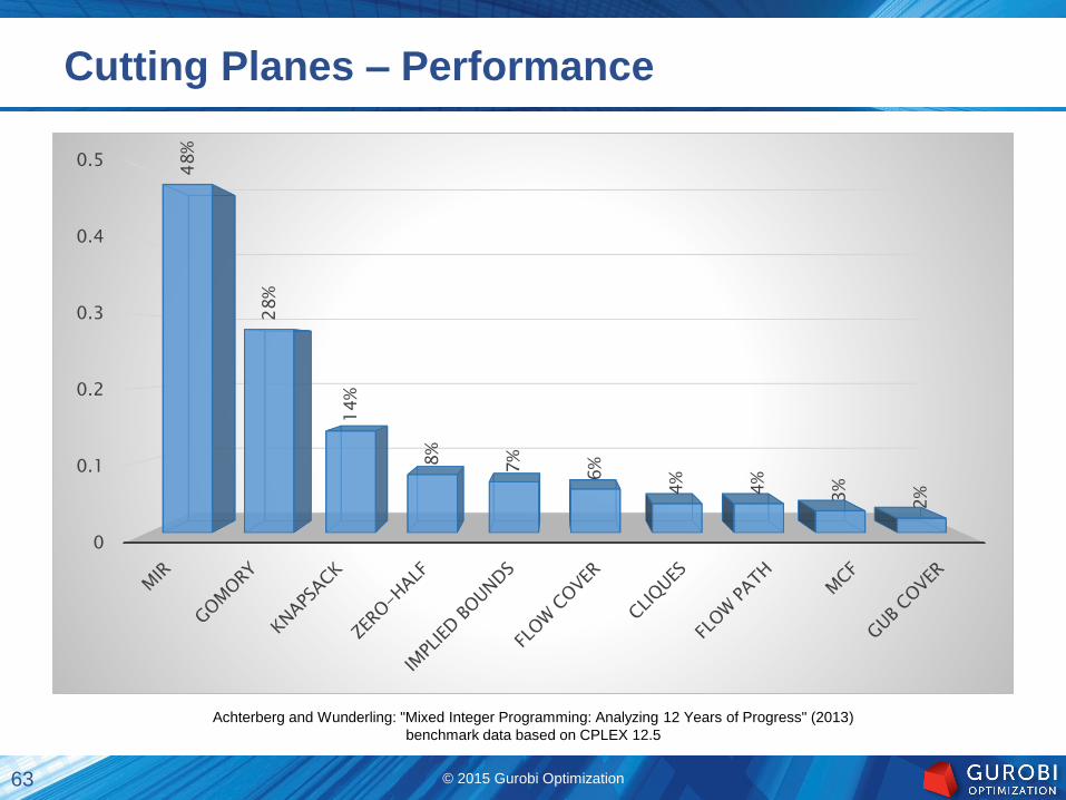
48%

28%

14%

8%

7%

6%

4%

4%

3%

2%

Achterberg and Wunderling: "Mixed Integer Programming: Analyzing 12 Years of Progress" (2013)

benchmark data based on CPLEX 12.5


MIP Building Blocks

Presolve





Cutting planes




Primal heuristics



MIP – Branching

objective


MIP – Branching

objective

P1 P2


MIP – Branching

objective

P1 P2

another improvement in dual bound


LP based Branch-and-Bound

Root

Solve LP relaxation:

v=3.5 (fractional)



Root



Root

Integer

Upper Bound


Remarks:(1) GAP = 0 Proof of optimality(2) In practice: good quality solution often enough


G

A

P

Root

Integer

Infeas

Infeas

Lower Bound

Upper Bound

Infeas


Solving a MIP Model

Solution

Bound

Obje

cti

ve

Time


Branching Variable Selection

Given a relaxation solution x*

◦ Branching candidates:

Integer variables xj that take fractional values

xj = 3.7 produces two child nodes (x ≤ 3 or x ≥ 4)

◦ Need to pick a variable to branch on

Choice is crucial in determining the size of the overall search tree


Branching Variable Selection

What’s a good branching variable?

◦ Superb: fractional variable infeasible in both branch directions

◦ Great: infeasible in one direction

◦ Good: both directions move the objective

Expensive to predict which branches lead to infeasibility or big objective moves

◦ Strong branching

Truncated LP solve for every possible branch at every node

Rarely cost effective

◦ Need a quick estimate


Pseudo-Costs

Use historical data to predict impact of a branch:

◦ Record cost(xj) = Δobj / Δxj for each branch

◦ Store results in a pseudo-cost table

Two entries per integer variable

Average down cost

Average up cost

◦ Use table to predict cost of a future branch

c*=13x* = 2.7


Pseudo-Costs





Average down cost

Average up cost


c*=13

c*=20 c*=19

x* = 2.7

down pseudo-cost update:

∆obj/∆x = 7/0.7 = 10

up pseudo-cost update:

∆obj/∆x = 6/0.3 = 20


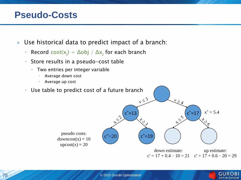
Pseudo-Costs





Average down cost

Average up cost


c*=13

c*=20 c*=19

c*=17

pseudo costs:

downcost(x) = 10

upcost(x) = 20

x* = 5.4

down estimate:c' = 17 + 0.4 ⋅ 10 = 21

up estimate:c' = 17 + 0.6 ⋅ 20 = 29


Pseudo-Costs Initialization

What do you do when there is no history?

◦ E.g., at the root node

Initialize pseudo-costs [Linderoth & Savelsbergh, 1999]

◦ Always compute up/down cost (using strong branching) for new fractional variables

Initialize pseudo-costs for every fractional variable at root

Reliability branching [Achterberg, Koch & Martin, 2005]

◦ Do not rely on historical data until pseudo-cost for a variable has been recomputed r times


Branching Rules – Performance

0

1

2

3

4

5

6

7

8

MOST FRACTIONAL RANDOM PSEUDO-COSTS WITH

SB INIT

RELIABILITY

0%

2%

548%

736%


benchmark data based on CPLEX 12.5

Achterberg, Koch, and Martin: "Branching Rules Revisited" (2005)


MIP Building Blocks

Presolve





Cutting planes




Primal heuristics



Primal Heuristics Explained on Twitter


Primal Heuristics

Try to find good integer feasible solutions quickly

◦ Better pruning during search due to better bound

◦ Reach desired gap faster

◦ Often important in practice: quality of solution after fixed amount of time

Start heuristics

◦ Try to find integer feasible solution, usually "close" to LP solution

Rounding heuristics: round LP solution to integral values Potentially, try to fix constraint infeasibilities

Fix-and-dive heuristics: fix variables, propagate, resolve LP

Feasibility pump: push LP solution towards integrality by modifying objective

RENS: Solve sub-MIP in neighborhood of LP solution

Improvement heuristics

◦ Given integer feasible solution, try to find better solution

1-Opt and 2-Opt: Modify one or two variables to get better objective

Local Branching: Solve sub-MIP in neighborhood of MIP solution

Mutation: Solve sub-MIP in neighborhood of MIP solution

Crossover: Solve sub-MIP in neighborhood of 2 or more MIP solutions

RINS: Solve sub-MIP in neighborhood of LP and MIP solution


Primal Heuristics – Performance

0.00

0.02

0.04

0.06

0.08

0.10

0.12

0.14

4%

4%

12%

4%

6%

3%

2%

2%

1%

2%

2%

Berthold: "Primal Heuristics for Mixed Integer Programs" (2006)

benchmark data based on SCIP 0.82b


Primal Heuristics – Measuring Performance

Is time to optimality a good measure to assess impact of heuristics?

◦ Goal of heuristics is to provide good solutions quickly

◦ Faster progress in dual bound due to additional pruning is only secondary

◦ Often important for practitioners:

Find any feasible solution quickly to validate that model is reasonable

Find good solution in reasonable time frame

Primal gap: 𝛾𝑝 𝑥 =𝑐𝑇𝑥∗−𝑐𝑇 𝑥

𝑚𝑎𝑥 𝑐𝑇𝑥∗ , 𝑐𝑇 𝑥

Primal gap function: 𝑝 𝑡 = 1, if no incumbent until time 𝑡

𝛾𝑝 𝑥 𝑡 , with 𝑥 𝑡 being incumbent at time 𝑡

Primal integral: 𝑃 𝑇 = 𝑡=0

𝑇𝑝 𝑡 𝑑𝑡


Solution

Bound

Primal IntegralO

bje

cti

ve

Time

cTx*

P(T)


Primal Heuristics – Performance

0

10

20

30

40

50

60

70

80

90

HEURISTICS ON HEURISTICS OFF

9.3

35.3

78.9

90

8.9

17.2

time to first (s) time to opt (s) primal integral (%)

Berthold (2014): "Heuristic algorithms in global MINLP solvers"

benchmark data based on SCIP 3.0.2


Putting It All Together


Branch-and-Cut

Presolving Node Selection

LP Relaxation

Cutting Planes

Node Presolve

Branching

Heuristics