mixed and blume–capel ising ferrimagnetic system on the bethe lattice

ARTICLE IN PRESS

Physica A 345 (2005) 48–60

0378-4371/$ -

doi:10.1016/j

�Correspo

E-mail ad

www.elsevier.com/locate/physa

Mixed spin- 12and spin- 3

2Blume–Capel Ising

ferrimagnetic system on the Bethe lattice

Erhan Albayrak�, Akkadin Alc- i

Department of Physics, Erciyes University, 38039 Kayseri, Turkey

Available online 21 July 2004

Abstract

We present the exact formulation for the mixed spin-12

and spin-32

Blume–Capel Ising

ferrimagnetic system on the Bethe lattice by the use of exact recursion relations. The exact

expressions for the magnetization, quadrupole moment, Curie temperature and free energy are

found and the phase diagrams are illustrated on the Bethe lattice with the coordination

numbers q ¼ 3, 4, 5 and 6. It is found that the phase diagram of this mixed spin system only

presents second-order phase transitions. The thermal variation of the magnetization belonging

to each sublattice and the net magnetization are also presented.

r 2004 Elsevier B.V. All rights reserved.

PACS: 05.50.+q; 05.70.Fh; 64.60.Cn; 75.10.Hk

Keywords: Recursion relations; Bethe lattice; Mixed-spin; Phase diagram

1. Introduction

The two-sublattice mixed spin-SA and spin-SB (SAaSB) systems are of interestsince they present less translational symmetry than their single counterparts andexhibit many new phenomena that cannot be observed in the single-spin Ising model.These systems are well adopted to study a certain type of ferrimagnetism which are

see front matter r 2004 Elsevier B.V. All rights reserved.

.physa.2004.04.134

nding author.

dress: [email protected] (E. Albayrak).

www.elsevier.com/locate/physa

ARTICLE IN PRESS

E. Albayrak, A. Alc- i / Physica A 345 (2005) 48–60 49

of great interest because of their interesting and possible useful properties for thetechnological applications as well as academic researchers. For example, it hasbeen shown experimentally that the MnNi (EDTA)-6H2O complex is a mixed-spinsystem [1].

The most extensively studied mixed-spin Ising models consist of half-integerand integer spins, i.e., spin-1

2and spin-1 and, spin-1 and spin-3

2, etc. The mixed

spin-12

and spin-1 system has been studied by the renormalization-group (RG)technique [2], high-temperature series expansions [3], the free-fermionapproximation [4], the Bethe-Peierls (BP) method [5], the framework of theeffective-field theory (EFT) [6,7], the mean-field approximation (MFA) [8,9],the finite cluster approximation (FCA) [10], the Monte-Carlo (MC) simulation[11,12], the mean-field renormalization-group (MFRG) [13], a numericaltransfer matrix study [12] and the cluster variation method in pair-approximation(CVMPA) [14]. Moreover, this mixed-spin model was also exactly solved on aBethe lattice by using a discrete nonlinear map [15] and by using the exactrecursion relations [16], leading to the same results of a recent CVMPAcalculation [14]. Several theoretical studies of the two-sublattice mixed spin-1 andmixed spin-3

2Ising models have been reported; based on the EFT with correlations

that correctly incorporates the single-site kinematic relations of the spin operatorson a honeycomb lattices [17], on a square lattice [18] and, on the square andsimple cubic lattices [19], within the mean-field theory based on the Bogoliubovinequalityfor the Gibbs free energy [20], by a cluster variational theory withinthe pair approximation [21] and by using the exact recursion relations on theBethe lattice [22].

Despite all these works, the half-integer or integer mixed-spin systems have notreceived enough attention. We could only report a few works for the mixedspin-1

2and spin-3

2Ising system; the transverse Ising model with a crystal field within

the framework of the EFT with correlations on the honeycomb lattice [23], on asquare lattice by using the EFT [24,25] and again on a square lattice with a MCalgorithm [26].

Therefore, the main purpose of this work is to present an exact formulation of themixed spin-1

2and spin-3

2Ising system on a Bethe lattice using the exact recursion

equations [27] and to obtain the phase diagrams for various values of thecoordination numbers q on the ðkTc

J; D

JÞ plane. The thermal variation of the

magnetization for each sublattice, i.e., for spin-12

and for spin-32, and the net

magnetization are also studied and illustrated for q ¼ 6.The rest of the paper is arranged as follows. In Section 2, the formulation

of the problem is given and the exact expressions for the magnetizationand the quadrupolar moment are obtained. The exact expressions for thesecond-order phase transition temperatures (Curie temperature) and thefree energy are obtained in Section 3. The thermal variations of magneti-zations belonging to each sublattice and the net magnetization for q ¼ 6and the phase diagram on the ðkTc

J; D

JÞ plane for q ¼ 3, 4, 5 and 6 are presented

in Section 4. Finally, the last section is devoted to a brief summary and aconclusion.

ARTICLE IN PRESS

E. Albayrak, A. Alc- i / Physica A 345 (2005) 48–6050

2. The formulation of the problem

The Hamiltonian of the mixed-spin Blume–Capel (BC) model on the Bethe latticeG is given by

H ¼ �JXhi;ji

si sj � DX

i

s2j ; ð1Þ

where each si located at site i is a spin of kind 1 and each sj located at site j is a spinof kind 2, on the Bethe lattice. In the case of mixed spins, the Bethe lattice isarranged such that it contains two different kinds of spins. Therefore, the centralspin is chosen to be kind 1, the next generation spins are of kind 2, and the nextgeneration spins are again kind 1, and so on to infinity, illustrated in Fig. 1. The firstsum runs over all nearest-neighbor pairs of G. J and D are the bilinear exchange andcrystal-field interactions, respectively. The calculation on the Bethe lattice is donerecursively [27].

In order to calculate all the function of the interest, we need to calculate thepartition function and is given by the definition as

Z ¼X

e�bH ¼XSpc

PðSpcÞ ¼Xfs;sg

exp b JXhi;ji

si sj þ DX

j

s2j

!" #; ð2Þ

where PðSpcÞ can be thought of as an unnormalized probability distribution over thespin-configurations, Spc (e.g. fs; sg), and si and sj indicates the spin-values at site i

σ2

σ2

σ2 σ2

σ2σ0

σ2

s3

s3

s3

s3

s3 s3

s3

s3

s3s1 s1

s1

s3 s3

Fig. 1. Bethe lattice, or regular tree, of coordination number 3 for mixed spin-12

and spin-32

BC Ising

system. The Bethe lattice is arranged such that the central spin so (the filled circle) is spin-12, the next

generation spins s1 (open circles) are spin-32, and the next generation spins s2 (filled circles) are again spin-1

2,

and so on to infinity.

ARTICLE IN PRESS


and site j, respectively. If the Bethe lattice is cut in some central point with a spin so,spin of kind 1, then it splits up into q identical branches, i.e., disconnected pieces.Each of these is a rooted tree at the central spin so. This implies that PðfsoÞg, i.e.,Spc ¼ fsog, is a spin-configuration with the spin value so at the central site, can bewritten as

PðfsogÞ ¼Yq

k¼1

QnðsojfsðkÞ1 gÞ ; ð3Þ

where fsðkÞ1 g indicates the spin-configurations of the kth branch of the Cayley tree

starting with sðkÞ1 (n � 2 variables, tðlÞ2 ; rðmÞ

3 , etc., following) other than the central spinso, the suffix n denotes the fact that the sub-tree has n-shells, i.e., n steps from theroot to the boundary sites, and

QnðsojfsðkÞ1 gÞ ¼ exp b Jsos

ðkÞ1 þ bDðs

ðkÞ1 Þ

2þ J

Xhi;jið0X20Þ

si sj þ DX

jð0X20Þ

s2j

0@

1A

24

35 ;ð4Þ

where ð0X20Þ means that the first two digits are left out in the summations and si andsj are the spins of the site i and j of the sub-tree (other than the central spin so, whichis a spin of kind 1). Site 1 with spin of kind 2, i.e., s

ðkÞ1 , is the site next to the central

point 0. The first summation in Eq. (4) is over all edges of the sub-tree other than theedge (0, 1) and the summation over i is over all sites with spin of kind 1 other thanthe central site. Now if the sub-tree, say the upper sub-tree, is cut at the site 1 next to0, then it also decomposes into q pieces: one being ‘‘trunk’’ (0,1) and the rest are theidentical branches. Each of these branches is a sub-tree like the original, but withn � 1 shells and q � 1 neighbors. Thus

QnðsojfsðkÞ1 gÞ ¼ exp½bJsos

ðkÞ1 þ bDðs

ðkÞ1 Þ

2 �Yq�1

l¼1

Q0n�1ðs

ðkÞ1 jftðlÞ2 gÞ ; ð5Þ

where ftðlÞ2 g denotes the spin-configurations (other than sðkÞ1 ) on the lth branch of the

upper sub-tree and the prime over Qn�1 is used to distinguish the sublattice withspin-1

2from the sublattice with 3

2. If the upper sub-tree is cut at site 2 with a spin of

kind 1, i.e., s2, next to site 1, then it again decomposes into q pieces: one again beingthe second trunk (1, 2) and the rest are the identical branches, again with n � 1 shellsand q � 1 neighbors. So

Q0n�1ðs

ðkÞ1 jftðlÞ2 gÞ ¼ exp½bJs1s2 �

Yq�1

m¼1

Qn�2ðtðlÞ2 jfr

ðmÞ

3 gÞ ; ð6Þ

where frðmÞ

3 g denotes again the spin-configurations (other than tðlÞ2 ) on the next mthbranch of the upper subsub-tree. In this way, one should take n steps from root tothe boundary on the Bethe lattice, i.e., in the thermodynamic limit n ! 1. As aresult, the Bethe lattice is set up in such a way that the central spin so is being spin ofkind 1 with q-neighbors of spin of kind 2, i.e., s1, the next generation s1 of kind 2 has

ARTICLE IN PRESS


q � 1 neighbors spin with kind 1, s2, and the next generation with spin s2 of kind 1has q � 1 neighbors of spin of kind 2, s3, and so on to infinity. Therefore, the newformulation includes all the interactions of spin of kind 1 with spin of kind 2 andwith the crystal-field interaction. Now defining

gnðsoÞ ¼Xfs1g

Qnðsojfs1gÞ ; ð7Þ

and using it in Eq. (2) the partition function for the central spin so takes the form

Z ¼Xfsog

½gnðsoÞ q : ð8Þ

On the other hand, if so is the spin of kind 1 at the central site 0, then themagnetization or the dipole and the quadrupolar order parameters are given by thedefinition

M ¼ Z�1Xfsog

so PðfsogÞ; Q ¼ Z�1Xfsog

s2o PðfsogÞ ; ð9Þ

respectively. PðfsogÞ and Z are given by Eqs. (3) and (8), respectively, and so is thespin of kind 1 at the central site 0. Using Eqs. (3)–(8), one can easily calculate themagnetization or the dipole moment M as

M ¼ Z�1Xso

so½gnðsoÞ q ; ð10Þ

and similarly the quadrupolar order parameter Q as

Q ¼ Z�1Xso

s2o½gnðsoÞ

q : ð11Þ

The above formulation is the detailed generalization of the mixed spin BC Isingferrimagnetic system on the Bethe lattice and it is well-known that the single-ionanisotropy term D is neutral for the spin-1

2, therefore, it is obvious that s represents

spin-12and s represents spin-3

2. Now, we are ready to obtain the necessary formulation

for the special case of the mixed spin-12and spin-3

2BC Ising ferrimagnetic system.

In the case of mixed spin-12and spin-3

2, each si located at site i is a spin-1

2and can

take the values �12and each sj located at site j is a spin-3

2and can take the values �3

2

and �12 on the Bethe lattice. In this formulation the Bethe lattice is arranged such

that the central spin is spin-12, the next generation is spin-3

2, and the next generation is

again spin-12, and so on to infinity, see Fig. 1. It is important to note here that the

choice of the central spin, i.e., whether spin-12or spin-3

2, does not affect the results and

both choice leads to same physical conclusions [22].Since the central spin so is chosen to be the spin-1

2, which can have the values �1

2,

the partition function can be calculated using Eqs. (3), (7) and (8) as

Z ¼ gn12

� �� qþ gn �1

2

� �� q: ð12Þ

ARTICLE IN PRESS


M and Q can be written for the central spin so by using Eqs. (3), (10)–(12) as

M ¼

12½gnð

12Þ

q � 12½gnð�

12Þ

q

½gnð12Þ q þ ½gnð�

12Þ q

; ð13Þ

Q ¼

14½gnð

12Þ q þ 1

4½gnð�

12Þ q

½gnð12Þ q þ ½gnð�

12Þ q

; ð14Þ

respectively.In order to calculate M and Q explicitly from Eqs. (13) and (14), first we need to

sum Eq. (6) over all the spins, i.e., s1 is spin-32and s2 is spin 1

2, together with Eq. (7),

g0n�1ðs1Þ ¼

Xs2

exp½bJs1s2 ½gn�2ðs2Þ q�1 : ð15Þ

Since s1 can take the values �32and �1

2and s2 can take the values �1

2, one can

obtain four different g0nðs1Þ for four possible values of s1, then for s1 ¼ �3

2

g0n�1 �

3

2

� �¼ exp �

3bJ

4

� �gn�2

1

2

� �� q�1

þ exp �3bJ

4

� �gn�2 �

1

2

� �� q�1

;

ð16Þ

and for s1 ¼ � 12

g0n�1 �

1

2

� �¼ exp �

bJ

4

� �gn�2

1

2

� �� q�1

þ exp �bJ

4

� �gn�2 �

1

2

� �� q�1

: ð17Þ

Now in order to calculate the gnðsoÞ, we need to consider Eq. (5) together withEq. (7), summing over all so, i.e., a spin-1

2, and s1, which is a spin-3

2, we obtain

gnðsoÞ ¼X

s1

exp½bJsos1 þ bDs21 ½g0n�1ðs1Þ

q�1 ; ð18Þ

and since so can have only two values, i.e., �12, we get two different gnðsoÞ for two

possible values of so

gn �1

2

� �¼ exp �

3bJ

4þ

9bD

4

� �g0

n�1

3

2

� �� q�1

þ exp �3bJ

4þ

9bD

4

� �g0

n�1 �3

2

� �� q�1

þ exp �bJ

4þ

bD

4

� �g0

n�1

1

2

� �� q�1

þ exp �bJ

4þ

bD

4

� �g0

n�1 �1

2

� �� q�1

: ð19Þ

Now, we are ready to introduce the recursion relations as

X n ¼gnð

12Þ

gnð�12Þ; Y n ¼

g0nð

32Þ

g0nð�

12Þ; Zn�1 ¼

g0nð�

32Þ

g0nð�

12Þ; W n�1 ¼

g0nð

12Þ

g0nð�

12Þ: ð20Þ

ARTICLE IN PRESS


Thus we can obtain a set of four recursion relations from which the dipole(magnetization) and quadrupolar order parameters can be found. Therefore, therecursion equations are found by substituting Eqs. (15)–(19) into Eq. (20) as

X n ¼e

b0ð3þ9dÞ4

h iY

q�1n�1 þ e

b0ð�3þ9dÞ4

h iZ

q�1n�1 þ e

b0ð1þdÞ4

h iW

q�1n�1 þ e

b0ð�1þdÞ4

h i

eb0ð�3þ9dÞ

4

h iY

q�1n�1 þ e

b0ð3þ9dÞ4

h iZ

q�1n�1 þ e

b0ð�1þdÞ4

h iW

q�1n�1 þ e

b0ð1þdÞ4

h i ; ð21Þ

Y n�1 ¼e

3b0

4

h iX

q�1n�2 þ e

�3b0

4

h i

e�b0

4

h iX

q�1n�2 þ e

b0

4

h i ; ð22Þ

Zn�1 ¼e

�3b0

4

h iX

q�1n�2 þ e

3b0

4

h i

e�b0

4

h iX

q�1n�2 þ e

b0

4

h i ; ð23Þ

W n�1 ¼e

b0

4

h iX

q�1n�2 þ e

�b0

4

h i

e�b0

4

h iX

q�1n�2 þ e

b0

4

h i ; ð24Þ

where b0 ¼ bJ and d ¼ DJ.

It should be mentioned that the values of X , Y , Z and W have no direct physicalsense, but one can express in terms of X , Y , Z and W all thermodynamic functionsof interest. The sublattice with spin-1

2is a two-state system, i.e., spin-up and spin-

down, therefore, for the definition of this sublattice one needs only one order-parameter, the magnetization. Thus, the magnetization for the central spin withspin-1

2is obtained in terms of recursion relations by using Eqs. (13) and (20) as

M1=2 ¼1

2

X qn � 1

X qn þ 1

: ð25Þ

It should be mentioned that in order to obtain the magnetization and quadrupolemoment for the central spin with spin-3

2, one does not need to carry out all these

formulation which are simply by using Eq. (9) and Eqs. (22)–(24)

M3=2 ¼

32 e

9b0d4

h iðY

qn�1 � Z

qn�1Þ þ

12 e

b0d4

h iðW

qn�1 � 1Þ

e9b0d4

h iðY

qn�1 þ Z

qn�1Þ þ e

b0d4

h iðW

qn�1 þ 1Þ

; ð26Þ

Q3=2 ¼

94e

9b0d4

h iðY

qn�1 þ Z

qn�1Þ þ

14e

b0d4

h iðW

qn�1 þ 1Þ

e9b0d4

h iðY

qn�1 þ Z

qn�1Þ þ e

b0d4

h iðW

qn�1 þ 1Þ

: ð27Þ

ARTICLE IN PRESS


From the recursion relations, namely Eqs. (21)–(24), X n, Y n, Zn and W n can beobtained, using the values of these recursion relations in Eqs. (25)–(27) and varyingthe system parameters, i.e., d ¼ D

Jand b0 ¼ J

kT, one can study the behavior of the

order parameters as a function of temperature for various values of the couplingconstant D

Jand coordination number q. Therefore, by studying the thermal

variations of magnetizations M1=2 or M3=2, one can obtain the phase diagrams forthe mixed spin-1

2and spin-3

2BC model on the ðkTc

J; D

JÞ plane for various values of D

Jand

q. It should also be mentioned that the choice of the central spin has no effect on thecritical temperatures, that is they lead to the same phase diagrams.

3. The second- and first-order phase transition temperatures

In order to obtain the phase diagrams of the mixed spin-12and spin-3

2system, one

needs to find the places of the second-order (Curie temperature) and the first-orderphase transition temperatures on the ðkTc=J;D=JÞ plane. Therefore, to obtain anexact expression for the second-order phase transition temperature one needs tosearch for the temperature at which the magnetization goes to zero continuously. So,by setting Eq. (25) or Eq. (26) to be equal to zero and observing the behavior of therecursion relations, we have obtained that the recursion relations must satisfy theconditions:

X n ¼ 1; Y n�1 ¼ Zn�1; W n�1 ¼ 1 ð28Þ

which have a simple interpretation as follows: At the Curie temperature themagnetization must be equal to zero, therefore the probability of spins being up andspins being down must be equal which implies that gnðþ

12Þ ¼ gnð�

12Þ for spin-1

2and

g0nðþ

12Þ ¼ g0

nð�12Þ and g0

nðþ32Þ ¼ g0

nð�32Þ for spin-3

2. It should be mentioned that they

also satisfy the recursion relations and Eq. (28) at the Curie temperature. Deep insidethe Bethe lattice, i.e., far from the boundary sites all sites with spin-1

2and all sites

with spin-32are equivalent, thus one can omit the suffix n, hence X ¼ 1, Y ¼ Z and

W ¼ 1. Now, we may obtain an equation for the second-order phase transitiontemperature by using Eq. (21) or Eq. (22) as

Y ¼ Z ¼cosh

3bc4

� �cosh

bc4

� � ð29Þ

which could be solved numerically to obtain the second-order phase transition or theCurie temperatures. Instead of obtaining the Curie temperatures by using the aboveequation, first we have obtained the numerical values of the recursion relations X , Y ,Z and W for various values of D

Jand q iteratively from Eqs. (21)–(24) and then used

these values in Eqs. (25) and (26) to obtain the magnetizations belonging to eachsublattice, i.e., M1=2 for spin-1

2and M3=2 for spin-3

2, respectively. Then, the Curie

temperature is the temperature when either of these sublattice magnetizations goes tozero continuously, since both must lead to the same critical temperatures.

ARTICLE IN PRESS


Using Eqs. (27) and (28), we have also obtained an equation to study the behaviorof the quadrupolar order-parameter as a function of the critical temperatures as

Q3=2 ¼

94e

9bcd4

h iY q þ 1

4e

bcd4

h i

e

9bcd4

h iY q þ e

bcd4

h i ; ð30Þ

where Y is given by Eq. (29).In order to find the places of the first-order phase transition temperatures on the

(kTcJ; D

J) plane, we need the free-energy expression, so using the definition of the free

energy F ¼ �kT ln Z and Eqs. (12), (15)–(19) in thermodynamic limit as n ! 1,we have obtained the free energy expression in terms of the recursion relations as

F ¼ �1

b01

2 � qln e b0 �

34þ

9d4

� �� Y

q�1n�1 þ e b0 3

4þ

9d4

� �� Z

q�1n�1 þ e b0 �

14þ

d4

� �� W

q�1n�1

��

þe b0 14þ

d4

� �� þ

q � 1

2 � qln e

�b0

4

h iX q�1

n þ eb0

4

h i" #þ ln X q

n þ 1� �#

: ð31Þ

The first-order phase transition temperatures are determined from a free energyanalysis. It should be mentioned that in solving the recursion relations, i.e., Eqs.(21)–(24), one has to assign an initial value for each of X , Y , Z and W . Therefore,varying the initial values may result in different solutions for all the thermodynamicfunctions including the free energy. As a result, the temperature at which the freeenergy values are equal to each other is the first-order phase transition temperature.

We can now obtain the thermal variations of the sublattice magnetizations and thenet magnetization, defined as MNET ¼j M3=2 � M1=2 j since Jo0 for the ferrimag-netic ordering the sublattice magnetizations directed oppositely, therefore bystudying the thermal variations of the magnetizations one can obtain the phasediagrams of the mixed spin-1

2and spin-3

2BC Ising ferrimagnetic system on the ðkTc

J; D

JÞ

plane for various values of the coordination number q. The discussion of the thermalvariations of the magnetizations and the phase diagrams are given in the nextSection.

4. Thermal variations of magnetizations and phase diagrams

The temperature change of the sublattice magnetizations and the net magnetiza-tion are studied for various values of D

Jand coordination number q, because of the

similarity of the thermal variations of the magnetizations the results are onlyillustrated for q ¼ 6.

The sublattice magnetizations M1=2 and M3=2 for the mixed BC Isingferrimagnetic system, Jo0, are obtained numerically from Eqs. (25), (26) and therecursion relations and shown only for q ¼ 6 (See Fig. 2). Since the system isferrimagnetic the sublattice magnetizations are directed oppositely. In the figure,while the negative magnetization axis shows the sublattice magnetization for spin-1

2,

ARTICLE IN PRESS

kT/J

0.5 1.0 1.5 2.0 2.5 3.0 3.5 4.0

-5

-1

0

1.55

q=61.50

1.25

1.00

0.75

0.50

0.25

0.00

-0.25

-0.50

-0.750.0

M3/

2M

1/2

-0.5

-1.9

-2.4

-1.5

-1.6

Fig. 2. The thermal variations of the sublattice magnetizations. The positive magnetization axis denotes

the sublattice magnetization M3=2 for spin-32and the negative axis for the sublattice magnetization M1=2

for spin-12for the ferrimagnetic system with q ¼ 6. The lines are labelled with the values of D

J.


the positive axis shows the sublattice magnetization for spin-32

and the lines arelabelled with the values of D

J. As seen in the figure both sublattice magnetizations,

M1=2 and M3=2, go to zero continuously, indicating the existence of the second-orderphase transition temperature, and terminate at the same critical temperature.Therefore, in obtaining the phase diagrams one can use either of the sublatticemagnetizations. We have also studied the thermal variations of the sublatticemagnetizations for q ¼ 3, 4, and 5, and observed that as q increases the second-orderphase transition temperatures occur at higher temperatures. As a final note weshould mention that if one compares Fig. 2 of this work with Figs. 1a, b of Jianget al. [23] and with Fig. 4 of Buendia et al. [26], an overall agreement is found.

The net magnetization is defined as MNET ¼j M3=2 � M1=2 j and its thermalvariation is illustrated for q ¼ 6 only in Fig. 3. For spin-3

2the possible spin values are

�32and �1

2, therefore, for lower negative values and positive values of D

Jthe sublattice

magnetization M3=2 ¼ 3=2, i.e., MNET ¼ 1:0, and for higher negative values of DJthe

sublattice magnetization M3=2 ¼ 1=2, i.e., MNET ¼ 0:0, at zero temperature. Thus,for higher negative values of D

Jspins with spin-3

2acts like spins with spin-1

2, as a result

the net magnetization vanishes for DJffi �6:05 when q ¼ 6. For q ¼ 3, 4 and 5, the

net magnetization also vanishes when DJffi �2:58, �3:78, and �4:93, respectively. It

should also be mentioned that the net magnetization does also give the same criticaltemperatures as the sublattice magnetizations. The thermal behavior of the netmagnetization also shows an overall agreement with Fig. 1c of Ref. [23] and withFig. 3 of Ref. [26].

As a result of studying the thermal variations of the either of magnetizations,we are ready to obtain the phase diagram of the mixed spin-1

2and spin-3

2BC

Ising ferrimagnetic system on the ðkTcJ; D

JÞ plane for different coordination numbers,

i.e., q ¼ 3, 4, 5 and 6 (see Fig. 4). As we mentioned earlier the second-order phase

ARTICLE IN PRESS

kT/J

0.0

1.0

5.0

q=6

1.2

1.0

0.8

0.6

0.4

0.2

0.00.0 0.5 1.0 1.5 2.0 2.5 3.0 3.5 4.0

-0.5

-1.0

-1.4

-1.6

-1.9

-2.4

MN

ET

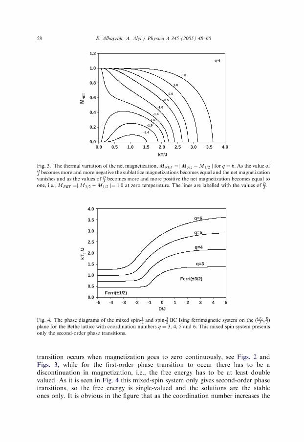
Fig. 3. The thermal variation of the net magnetization, MNET ¼j M3=2 � M1=2 j for q ¼ 6. As the value ofDJbecomes more and more negative the sublattice magnetizations becomes equal and the net magnetization

vanishes and as the values of DJ

becomes more and more positive the net magnetization becomes equal to

one, i.e., MNET ¼j M3=2 � M1=2 j¼ 1:0 at zero temperature. The lines are labelled with the values of DJ.

D/J0

q=3

q=4

q=5

q=6

1 2 3 4 5-5 -4 -3 -2 -1

4.0

3.5

3.0

2.5

2.0

1.5

1.0

0.5

0.0

kTc

/J

Ferri(±3/2)

Ferri(±1/2)

Fig. 4. The phase diagrams of the mixed spin-12and spin-3

2BC Ising ferrimagnetic system on the ðkTc

J; D

JÞ

plane for the Bethe lattice with coordination numbers q ¼ 3, 4, 5 and 6. This mixed spin system presents

only the second-order phase transitions.


transition occurs when magnetization goes to zero continuously, see Figs. 2 andFigs. 3, while for the first-order phase transition to occur there has to be adiscontinuation in magnetization, i.e., the free energy has to be at least doublevalued. As it is seen in Fig. 4 this mixed-spin system only gives second-order phasetransitions, so the free energy is single-valued and the solutions are the stableones only. It is obvious in the figure that as the coordination number increases the

ARTICLE IN PRESS


second-order phase transition occurs at higher critical temperatures. Since for thehigher negative values of D

Jspin-3

2acts like spin-1

2, therefore the phase diagram

presents two regions, ferrimagnetic (�12) and ferrimagnetic (�3

2). In Ref. [23]

the phase diagrams are only given for q ¼ 3 and with and without transversefield, therefore, when our figure is compared with their phase diagram with zerocrystal-field we see that the results are in well agreement. It should be mentionedthat the phase diagram for the square lattice in Ref. [26]also shows an overallagreement. In concluding this section we have to note that the phase diagram of thismixed-spin system is not very interesting, since it only gives second-order phasetransitions.

5. A brief summary and conclusion

The exact formulation for the mixed spin-12

and spin-32

Blume–Capel Isingferrimagnetic system on the Bethe lattice was studied by the use of exact recursionrelations. The exact expressions for the magnetization, quadrupole moment, Curietemperature and free energy are found in terms of the recursion relations. Thethermal variation of the magnetization belonging to each sublattice and the netmagnetization were studied in a great detail and the obtained results were comparedwith the results of Ref. [23] with zero transverse crystal-field and with Ref. [26], andan overall agreement was found. The phase diagrams on the ðkTc

J; D

JÞ plane for the

Bethe lattice with different coordination numbers, i.e., for q ¼ 3, 4, 5 and 6, werestudied by studying the thermal behavior of the sublattice magnetizations or the netmagnetization and free energy. As a result, it was found that the phase diagram ofthis mixed spin system presents only the second-order phase transitions.

References

[1] M. Drillon, E. Coronado, D. Beltran, R. Georges, J. Chem. Phys. 79 (1983) 449.

[2] S.L. Schofield, R.G. Bowers, J. Phys. A: Math. Gen. 13 (1980) 3697;

N. Benayad, J. Zittartz, Z. Phys. B. Condens. Matter 81 (1990) 107;

B. Boechat, R.A. Filgueiras, L. Marins, C. Cordeiro, N.S. Branco, Mod. Phys. Lett. B 14 (2000) 749;

B. Boechat, R.A. Filgueiras, C. Cordeiro, N.S. Branco, Physica A 304 (2002) 429.

[3] S.L. Schofield, R.G. Bowers, J. Phys. A: Math. Gen. 14 (1981) 2163;

B.Y. Yousif, R.G. Bowers, J. Phys. A: Math. Gen. 17 (1984) 3389.

[4] F.K. Tang, J. Phys. A: Math. Gen. 21 (1988) L1097.

[5] T. Iwashita, N. Uryu, Phys. Lett. A 96 (1983) 311;

T. Iwashita, N. Uryu, J. Phys. Soc. Japan 53 (1984) 721;

T. Iwashita, N. Uryu, Phys. Status Solidi b 125 (1984) 551.

[6] T. Kaneyoshi, Phys. Rev. B 34 (1986) 7866;

T. Kaneyoshi, J. Phys. Soc. Japan 56 (1987) 2675;

T. Kaneyoshi, J. Phys. Soc. Japan 58 (1989) 1755;

T. Kaneyoshi, J. Magn. Magn. Mater. 98 (2000) 201;

A.L. De Lima, B.D. Stogic, I.F. Fittipaldi, J. Magn. Magn. Mater. 226 (2001) 635.

[7] T. Kaneyoshi, Solid State Commun. 70 (1989) 975.

ARTICLE IN PRESS


[8] T. Kaneyoshi, E.F. Sarmento, I.F. Fittipaldi, Phys. Status Solidi b 150 (1988) 261;

J.A. Plascak, Physica A 198 (1993) 655

C. Ekiz, M. Keskin, Physica A (2002) in press.

[9] T. Kaneyoshi, J.C. Chen, J. Magn. Magn. Mater. 98 (1991) 201.

[10] N. Benayad, A. Klumper, J. Zittartz, A. Benyoussef, Z. Phys. B. Condens. Matter 77 (1989) 333, 339.

[11] G.M. Zhang, C.Z. Yang, Phys. Rev. B 48 (1993) 9452.

[12] G.M. Buendia, M.A. Novotny, J. Zhang, in: D.P. Landau, K.K. Mon, H.B. Schuttler (Eds.),

Springer Proceeds in Physics, Vol. 78, Computer Simulations in Condensed Matter Physics, Vol. VII,

Springer, Heidelberg, 1994, p. 223;

G.M. Buendia, M.A. Novotny, J. Phys.: Condens. Matter 9 (1997) 5951.

[13] H.F.V. De Resende, F.C. Sa Barreto, J.A. Plascak, Physica A 149 (1988) 606.

[14] J.W. Tucker, J. Magn. Magn. Mater. 195 (1999) 733.

[15] N.R. Da Silva, S.R. Salinas, Phys. Rev. B 44 (1991) 852.

[16] E. Albayrak, M. Keskin, J. Magn. Magn. Mater. 261 (2003) 196.

[17] A. Bobak, M. Jurcisin, Phys. Stat. Sol. b 204 (1997) 787;

A. Bobak, M. Jurcisin, Physica B 233 (1997) 187;

G.Z. Wei, Z.H. Xin, J. Wei, J. Magn. Magn. Mater. 204 (1999) 144;

A. Bobak, Physica A 258 (1998) 140;

J. Wei, G.Z. Wei, Z.H. Xin, Physica A 293 (2001) 455.

[18] Z.H. Xin, G.Z. Wei, T.S. Liu, J. Magn. Magn. Mater. 188 (1998) 65.

[19] A. Bobak, O.F. Abubrig, D. Horvath, J. Magn. Magn. Mater., in press.

[20] O.F. Abubrig, D. Horvath, A. Bobak, M. Jascur, Physica A 296 (2001) 437.

[21] J.W. Tucker, J. Magn. Magn. Mater. 237 (2001) 215.

[22] E. Albayrak, Int. J. Mod. Phys. 17 (2003) 1087;

E. Albayrak, Phys. Status Solidi b 239 (2003) 411.

[23] W. Jiang, G.Z. Wei, Z.H. Xin, Physica A 293 (2001) 455.

[24] N. Benayad, et al., Ann. Physik 5 (1996) 387.

[25] A. Bobak, M. Jurcisin, J. Phys. IV France 7 (1997) C1-179.

[26] G.M. Buendia, R. Cardano, Phys. Rev. B 59 (1999) 6784.

[27] R.J. Baxter, Exactly Solved Models in Statistical Mechanics, Academic Press Inc., New York, 1982.

mixed and blume–capel ising ferrimagnetic system on the bethe lattice

Documents