m.i.t. 18.03 ordinary di erential...
TRANSCRIPT

M.I.T. 18.03Ordinary Differential Equations
Notes and Exercises
Arthur Mattuck, Haynes Miller, David Jerison,Jennifer French, Jeremy Orloff

18.03 NOTES, EXERCISES, AND SOLUTIONS
NOTES
D. Definite Integral Solutions
G. Graphical and Numerical Methods
C. Complex Numbers
IR. Input Response Models
O. Linear Differential Operators
S. Stability
I. Impulse Response and Convolution
H. Heaviside Coverup Method
LT. Laplace Transform
CG. Convolution and Green’s Formula
LS1. Linear Systems: Review of Linear Algebra
LS2. Homogeneous Linear Systems with Constant Coefficients
LS3. Complex and Repearted Eigenvalues
LS4. Decoupling Systems
LS5. Theory of Linear Systems
LS6. Solution Matrices
GS. Graphing ODE Systems
GS78. Structural stability
LC. Limit Cycles
FR. Frequency Response
P. Poles and Amplitude Response
LA.1 Phase Plane and Linear Systems
LA.2 Matrix Multiplication, Rank, Solving Linear Systems
LA.3 Complete Solutions, Nullspace, Space, Dimension, Basis
LA.4 Inverses and Determinants
LA.5 Eigenvalues and Eigenvectors
LA.6 Diagonalization and Orthogonal Matrices
LA.7 Two Dimensional Dynamics
LA.8 Stability, Normal Modes
LA.9 Decoupling
LA.10 The Matrix Exponential
LA.11 Inhomogeneous Systems
PDE.1 Fourier’s Theory of Heat
PDE.2 Decoupling; Insulated ends
PDE.3 The Wave Equation

EXERCISES (exercises with * are not solved)
1. First Order ODE’s
2. Higher Order ODE’s
3. Laplace Transform
4. Linear Systems
5. Graphing Systems
6. Power Series
7. Fourier Series
8. Extra Problems9. Linear Algebra Exercises
10. PDE Exercises
SOLUTIONS TO 18.03 EXERCISES
c©A. Mattuck, Haynes Miller, David Jerison, Jennifer French andM.I.T. 2007, 2013, 2017

D. Definite Integral Solutions
You will find in your other subjects that solutions to ordinary differential equations(ODE’s) are often written as definite integrals, rather than as indefinite integrals. Thisis particularly true when initial conditions are given, i.e., an initial-value problem (IVP)is being solved. It is important to understand the relation between the two forms for thesolution.
As a simple example, consider the IVP
(1) y′ = 6x2, y(1) = 5.
Using the usual indefinite integral to solve it, we get y = 2x3 + c, and by substitutingx = 1, y = 5, we find that c = 3. Thus the solution is
(2) y = 2x3 + 3
However, we can also write down this answer in another form, as a definite integral
(3) y = 5 +
∫x
1
6t2dt .
Indeed, if you evaluate the definite integral, you will see right away that the solution (3) isthe same as the solution (2). But that is not the point. Even before actually integrating, youcan see that (3) solves the IVP (1). For, according to the Second Fundamental Theorem ofCalculus,
d
dx
∫x
a
f(t) dt = f(x) .
If we use this and differentiate both sides of (3), we see that y′ = 6x2, so that the firstpart of the IVP (1) is satisfied. Also the initial condition is satisfied, since
y(1) = 5 +
∫1
1
6t2 dt = 5 .
In the above example, the explicit form (2) seems preferable to the definite integral form(3). But if the indefinite integration that leads to (2) cannot be explicitly performed, wemust use the integral. For instance, the IVP
y′ = sin(x2), y(0) = 1
is of this type: there is no explicit elementary antiderivative (indefinite integral) for sin(x2);the solution to the IVP can however be written in the form (3):
y = 1 +
∫x
0
sin(t2) dt .
The most important case in which the definite integral form (3) must be used is inscientific and engineering applications when the functions in the IVP aren’t specified, butone still wants to write down the solution explicitly. Thus, the solution to the general IVP
(4) y′ = f(x), y(x0) = y0
may be written1

2 18.03 NOTES
(5) y = y0 +
∫x
x0
f(t) dt .
If we tried to write down the solution to (4) using indefinite integration, we would have tosay something like, “the solution is y =
∫f(x) dx + c, where the constant c is determined
by the condition y(x0) = y0” — an awkward and not explicit phrase.
In short, the definite integral (5) gives us an explicit solution to the IVP; the indefiniteintegral only gives us a procedure for finding a solution, and just for those cases when anexplicit antiderivative can actually be found.

G. Graphical and Numerical Methods
In studying the first-order ODE
(1)dy
dx= f(x, y),
the main emphasis is on learning different ways of finding explicit solutions. But you shouldrealize that most first-order equations cannot be solved explicitly. For such equations, oneresorts to graphical and numerical methods. Carried out by hand, the graphical methodsgive rough qualitative information about how the graphs of solutions to (1) look geometri-cally. The numerical methods then give the actual graphs to as great an accuracy as desired;the computer does the numerical work, and plots the solutions.
1. Graphical methods.
The graphical methods are based on the construction of what is called a direction field
for the equation (1). To get this, we imagine that through each point (x, y) of the plane isdrawn a little line segment whose slope is f(x, y). In practice, the segments are drawn inat a representative set of points in the plane; if the computer draws them, the points areevenly spaced in both directions, forming a lattice. If drawn by hand, however, they arenot, because a different procedure is used, better adapted to people.
To construct a direction field by hand, draw in lightly, or in dashed lines, what are calledthe isoclines for the equation (1). These are the one-parameter family of curves given bythe equations
(2) f(x, y) = c, c constant.
Along the isocline given by the equation (2), the line segments all have the same slope c;this makes it easy to draw in those line segments, and you can put in as many as you want.(Note: “iso-cline” = “equal slope”.)
The picture shows a direction field for the equation
y′ = x− y .
The isoclines are the lines x − y = c, two of whichare shown in dashed lines, corresponding to the valuesc = 0,−1. (Use dashed lines for isoclines).
Once you have sketched the direction field for the equa-tion (1) by drawing some isoclines and drawing in littleline segments along each of them, the next step is todraw in curves which are at each point tangent to the line segment at that point. Suchcurves are called integral curves or solution curves for the direction field. Their significanceis this:
(3) The integral curves are the graphs of the solutions to y′ = f(x, y) .
Proof. Suppose the integral curve C is represented near the point (x, y) by the graph ofthe function y = y(x). To say that C is an integral curve is the same as saying
0

G. GRAPHICAL AND NUMERICAL METHODS 1
slope of C at (x, y) = slope of the direction field at (x, y);
from the way the direction field is defined, this is the same as saying
y′(x) = f(x, y) .
But this last equation exactly says that y(x) is a solution to (1). �
We may summarize things by saying, the direction field gives a picture of the first-orderequation (1), and its integral curves give a picture of the solutions to (1).
Two integral curves (in solid lines) have been drawn for the equation y′ = x − y. Ingeneral, by sketching in a few integral curves, one can often get some feeling for the behaviorof the solutions. The problems will illustrate. Even when the equation can be solved exactly,sometimes you learn more about the solutions by sketching a direction field and some integralcurves, than by putting numerical values into exact solutions and plotting them.
There is a theorem about the integral curves which often helps in sketching them.
Integral Curve Theorem.
(i) If f(x, y) is defined in a region of the xy-plane, then integral curves of y′ = f(x, y)cannot cross at a positive angle anywhere in that region.
(ii) If fy(x, y) is continuous in the region, then integral curves cannot even be tangentin that region.
A convenient summary of both statements is (here “smooth”= continuously differentiable):
Intersection Principle
(4) Integral curves of y′ = f(x, y) cannot intersect wherever f(x, y) is smooth.
Proof of the Theorem. The first statement (i) is easy, for at any point (x0, y0) wherethey crossed, the two integral curves would have to have the same slope, namely f(x0, y0).So they cannot cross at a positive angle.
The second statement (ii) is a consequence of the uniqueness theorem for first-orderODE’s; it will be taken up then when we study that theorem. Essentially, the hypothesisguarantees that through each point (x0, y0) of the region, there is a unique solution to theODE, which means there is a unique integral curve through that point. So two integralcurves cannot intersect — in particular, they cannot be tangent — at any point wheref(x, y) has continuous derivatives.
Exercises: Section 1C

2 18.03 NOTES
2. The ODE of a family. Orthogonal trajectories.
The solution to the ODE (1) is given analytically by an xy-equation containing anarbitrary constant c; either in the explicit form (5a), or the implicit form (5b):
(5) (a) y = g(x, c) (b) h(x, y, c) = 0 .
In either form, as the parameter c takes on different numerical values, the correspondinggraphs of the equations form a one-parameter family of curves in the xy-plane.
We now want to consider the inverse problem. Starting with an ODE, we got a one-parameter family of curves as its integral curves. Suppose instead we start with a one-parameter family of curves defined by an equation of the form (5a) or (5b), can we find afirst-order ODE having these as its integral curves, i.e. the equations (5) as its solutions?
The answer is yes; the ODE is found by differentiating the equation of the family (5)(using implicit differentiation if it has the form (5b)), and then using (5) to eliminate thearbitrary constant c from the differentiated equation.
Example 1. Find a first-order ODE whose general solution is the family
(6) y =c
x− c(c is an arbitrary constant).
Solution. We differentiate both sides of (6) with respect to x, getting y′ = − c
(x− c)2.
We eliminate c from this equation, in steps. By (6), x− c = c/y, so that
(7) y′ = − c
(x− c)2= − c
(c/y)2= −y2
c;
To get rid of c, we solve (6) algebraically for c, getting c =yx
y + 1; substitute this for the
c on the right side of (7), then cancel a y from the top and bottom; you get as the ODEhaving the solution (6)
(8) y′ = −y(y + 1)
x.
Remark. The c must not appear in the ODE, since then we would not have a single ODE,but rather a one-parameter family of ODE’s — one for each possible value of c. Instead, wewant just one ODE which has each of the curves (5) as an integral curve, regardless of thevalue of c for that curve; thus the ODE cannot itself contain c.
Orthogonal trajectories.
Given a one-parameter family of plane curves, its orthogonal trajectories are anotherone-parameter family of curves, each one of which is perpendicular to all the curves in theoriginal family. For instance, if the original family consisted of all circles having center atthe origin, its orthogonal trajectories would be all rays (half-lines) starting at the origin.
Orthogonal trajectories arise in different contexts in applications. For example, if theoriginal family represents the lines of force in a gravitational or electrostatic field, its or-thogonal trajectories represent the equipotentials, the curves along which the gravitationalor electrostatic potential is constant.

G. GRAPHICAL AND NUMERICAL METHODS 3
In a temperature map of the U.S., the original family would be the isotherms, the curvesalong which the temperature is constant; their orthogonal trajectories would be the tem-
perature gradients, the curves along which the temperature is changing most rapidly.
More generally, if the original family is of the form h(x, y) = c, it represents the level
curves of the function h(x, y); its orthogonal trajectories will then be the gradient curves
for this function — curves which everywhere have the direction of the gradient vector ∇h.This follows from the 18.02 theorem which says the gradient ∇h at any point (x, y) isperpendicular to the level curve of h(x, y) passing through that point.
To find the orthogonal trajectories for a one-parameter family (5):
1. Find the ODE y′ = f(x, y) satisfied by the family.
2. The new ODE y′ = − 1
f((x, y)will have as its integral curves the orthogonal trajec-
tories to the family (5); solve it to find the equation of these curves.
The method works because at any point (x, y), the orthogonal trajectory passing through(x, y) is perpendicular to the curve of the family (5a) passing through (x, y). Therefore theslopes of the two curves are negative reciprocals of each other. Since the slope of the originalcurve at (x, y) is f(x, y), the slope at (x, y) of the orthogonal trajectory has to be −1/f(x, y).The ODE for the orthogonal trajectories then gives their slope at (x, y), thus it is
(9) y′ = − 1
f(x, y)ODE for orthogonal trajectories to (5a) .
More generally, if the equation of the original family is given implicitly by (5b), and itsODE is also in implicit form, the procedure and its justification are essentially the same:
1. Find the ODE in implicit form F (x, y, y′) = 0 satisfied by the family (5).2. Replace y′ by −1/y′; solve the new ODE F (x, y,−1/y′) = 0 to find the orthogonal
trajectores of the original family.
Example 2. Find the orthogonal trajectories to the family of curves y = c xn, where nis a fixed positive integer and c an arbitrary constant.
Solution. If n = 1, the curves are the family of rays from the origin, so the orthogonaltrajectories should be the circles centered at the origin – this will help check our work.
We first find the ODE of the family. Differentiating the equation of the family givesy′ = nc xn−1; we eliminate c by using the equation of the family to get c = y/xn andsubstituting this into the differentiated equation, giving
(10) y′ =n y
x(ODE of family); y′ = − x
n y(ODE of orthog. trajs.) .
Solving the latter equation by separation of variables leads first to n ydy = −xdx, thenafter integrating both sides, transposing, and multiplying through by 2, to the solution
(11) x2 + n y2 = k, (k ≥ 0 is an arbitrary non-negative constant; n is fixed.)
For different k-values, the equations (11) represent the family of ellipses centered at the
origin, and having x-intercepts at ±√k and y-intercepts at ±
√
k/n.If n = 1, these intercepts are equal, and the ellipses are circles centered at the origin, as
predicted.
Exercises: Section 1D-2

4 18.03 NOTES
3. Euler’s numerical method. The graphical method gives you a quick feel forhow the integral curves behave. But when they must be known accurately and the equationcannot be solved exactly, numerical methods are used. The simplest method is called Euler’s
method. Here is its geometric description.
We want to calculate the solution (integral curve) toy′ = f(x, y) passing through (x0, y0). It is shown as acurve in the picture.
We choose a step size h. Starting at (x0, y0), over theinterval [x0, x0 + h], we approximate the integral curve bythe tangent line: the line having slope f(x0, y0). (This isthe slope of the integral curve, since y′ = f(x, y).)
This takes us as far as the point (x1, y1), which is calculated by the equations (see thepicture)
x1 = x0 + h, y1 = y0 + h f(x0, y0) .
Now we are at (x1, y1). We repeat the process, using as the new approximation to theintegral curve the line segment having slope f(x1, y1). This takes us as far as the next point(x2, y2), where
x2 = x1 + h, y2 = y1 + h f(x1, y1) .
We continue in the same way. The general formulas telling us how to get from the (n−1)-stpoint to the n-th point are
(12) xn = xn−1 + h, yn = yn−1 + h f(xn−1, yn−1) .
In this way, we get an approximation to the integral curve consisting of line segmentsjoining the points (x0, y0), (x1, y1), . . . .
In doing a few steps of Euler’s method by hand, as you are asked to do in some of theexercises to get a feel for the method, it’s best to arrange the work systematically in a table.
Example 3. For the IVP: y′ = x2 − y2, y(1) = 0, use Euler’s method with step size .1to find y(1.2).
Solution. We use f(x, y) = x2 − y2, h = .1, and (12) above to find xn and yn:
n xn yn f(xn, yn) hf(xn, yn)0 1 0 1 .11 1.1 .1 1.20 .122 1.2 .22
Remarks. Euler’s method becomes more accurate the smaller the step-size h is taken.But if h is too small, round-off errors can appear, particularly on a pocket calculator.
As the picture suggests, the errors in Euler’s method will accumulateif the integral curve is convex (concave up) or concave (concave down).Refinements of Euler’s method are aimed at using as the slope for the linesegment at (xn, yn) a value which will correct for the convexity or concavity,and thus make the next point (xn+1, yn+1) closer to the true integral curve.We will study some of these. The book in Chapter 6 has numerical examplesillustrating Euler’ s method and its refinements.
Exercises: Section 1C

C. Complex Numbers
1. Complex arithmetic.
Most people think that complex numbers arose from attempts to solve quadratic equa-tions, but actually it was in connection with cubic equations they first appeared. Everyoneknew that certain quadratic equations, like
x2 + 1 = 0, or x2 + 2x+ 5 = 0,
had no solutions. The problem was with certain cubic equations, for example
x3 − 6x+ 2 = 0.
This equation was known to have three real roots, given by simple combinations of theexpressions
(1) A = 3
√
−1 +√−7, B = 3
√
−1−√−7;
one of the roots for instance is A+B: it may not look like a real number, but it turns outto be one.
What was to be made of the expressions A and B? They were viewed as some sortof “imaginary numbers” which had no meaning in themselves, but which were useful asintermediate steps in calculations that would ultimately lead to the real numbers you werelooking for (such as A+B).
This point of view persisted for several hundred years. But as more and more applicationsfor these “imaginary numbers” were found, they gradually began to be accepted as valid“numbers” in their own right, even though they did not measure the length of any linesegment. Nowadays we are fairly generous in the use of the word “number”: numbers of onesort or another don’t have to measure anything, but to merit the name they must belong to asystem in which some type of addition, subtraction, multiplication, and division is possible,and where these operations obey those laws of arithmetic one learns in elementary schooland has usually forgotten by high school — the commutative, associative, and distributivelaws.
To describe the complex numbers, we use a formal symbol i representing√−1; then a
complex number is an expression of the form
(2) a+ bi, a, b real numbers.
If a = 0 or b = 0, they are omitted (unless both are 0); thus we write
a+ 0i = a, 0 + bi = bi, 0 + 0i = 0 .
The definition of equality between two complex numbers is
(3) a+ bi = c+ di ⇔ a = c, b = d .
This shows that the numbers a and b are uniquely determined once the complex numbera+ bi is given; we call them respectively the real and imaginary parts of a+ bi. (It would bemore logical to call bi the imaginary part, but this would be less convenient.) In symbols,
(4) a = Re (a+ bi), b = Im (a+ bi)1

2 18.03 NOTES
Addition and multiplication of complex numbers are defined in the familiar way, makinguse of the fact that i2 = −1 :
Addition (a+ bi) + (c+ di) = (a+ c) + (b+ d)i(5a)
Multiplication (a+ bi)(c+ di) = (ac− bd) + (ad+ bc)i(5b)
Division is a little more complicated; what is important is not so much the final formulabut rather the procedure which produces it; assuming c+ di 6= 0, it is:
(5c) Divisiona+ bi
c+ di=
a+ bi
c+ di· c− di
c− di=
ac+ bd
c2 + d2+
bc− ad
c2 + d2i
This division procedure made use of complex conjugation: if z = a + bi, we define thecomplex conjugate of z to be the complex number
(6) z = a− bi (note that zz = a2 + b2 ).
The size of a complex number is measured by its absolute value, or modulus, defined by
(7) |z| = |a+ bi| =√
a2 + b2; (thus : zz = |z|2 ).
Remarks. For the sake of computers, which do not understand what a “formal expression”is, one can define a complex number to be just an ordered pair (a, b) of real numbers, anddefine the arithmetic operations accordingly; using (5b), multiplication is defined by
(a, b)(c, d) = (ac− bd, ad+ bc) .
Then if we let i represent the ordered pair (0, 1), and a the ordered pair (a, 0), it is easyto verify using the above definition of multiplication that
i2 = (0, 1)(0, 1) = (−1, 0) = −1 and (a, b) = (a, 0) + (b, 0)(0, 1) = a+ bi ,
and we recover the human way of writing complex numbers.
Since it is easily verified from the definition that multiplication of complex numbers iscommutative: z1z2 = z2z1, it does not matter whether the i comes before or after, i.e.,whether we write z = x + yi or z = x + iy. The former is used when x and y are simplenumbers because it looks better; the latter is more usual when x and y represent functions(or values of functions), to make the i stand out clearly or to avoid having to use parentheses:
2 + 3i, 5− 2πi; cos π2 + i sin π
2 , x(t) + i y(t) .
2. Polar representation.
Complex numbers are represented geometrically by points in the plane: the number a+ibis represented by the point (a, b) in Cartesian coordinates. When the points of the planerepresent complex numbers in this way, the plane is called the complex plane.
By switching to polar coordinates, we can write any non-zero complex number in analternative form. Letting as usual
x = r cos θ, y = r sin θ,
we get the polar form for a non-zero complex number: assuming x+ iy 6= 0,
(8) x+ iy = r(cos θ + i sin θ) .
When the complex number is written in polar form, we see from (7) that
r = |x+ iy|. (absolute value, modulus)

C. COMPLEX NUMBERS 3
We call θ the polar angle or the argument of x+ iy. In symbols, one sometimes sees
θ = arg (x+ iy) (polar angle, argument) .
The absolute value is uniquely determined by x+ iy, but the polar angle is not, since it canbe increased by any integer multiple of 2π. (The complex number 0 has no polar angle.) Tomake θ unique, one can specify
0 ≤ θ < 2π principal value of the polar angle.
This so-called principal value of the angle is sometimes indicated by writing Arg (x+ iy).For example,
Arg (−1) = π, arg (−1) = ±π,±3π,±5π, . . . .
Changing between Cartesian and polar representation of a complex number is essentially thesame as changing between Cartesian and polar coordinates: the same equations are used.
Example 1. Give the polar form for: −i, 1 + i, 1− i, −1 + i√3 .
Solution.
−i = i sin 3π2 1 + i =
√2 (cos π
4 + i sin π4 )
−1 + i√3 = 2 (cos 2π
3 + i sin 2π3 ) 1− i =
√2 (cos −π
4 + i sin −π4 )
The abbreviation cis θ is sometimes used for cos θ+ i sin θ; for students of science andengineering, however, it is important to get used to the exponential form for this expression:
(9) eiθ = cos θ + i sin θ Euler’s formula.
Equation (9) should be regarded as the definition of the exponential of an imaginary power.A good justification for it however is found in the infinite series
et = 1 +t
1!+
t2
2!+
t3
3!+ . . . .
If we substitute iθ for t in the series, and collect the real and imaginary parts of the sum(remembering that
i2 = −1, i3 = −i, i4 = 1, i5 = i, . . . ,
and so on, we get
eiθ =
(
1− θ2
2!+
θ4
4!− . . .
)
+ i
(
θ − θ3
3!+
θ5
5!− . . .
)
= cos θ + i sin θ ,
in view of the infinite series representations for cos θ and sin θ.
Since we only know that the series expansion for et is valid when t is a realnumber, the above argument is only suggestive — it is not a proof of (9). What itshows is that Euler’s formula (9) is formally compatible with the series expansionsfor the exponential, sine, and cosine functions.
Using the complex exponential, the polar representation (8) is written
(10) x+ iy = r eiθ
The most important reason for polar representation is that multiplication and divisionof complex numbers is particularly simple when they are written in polar form. Indeed, byusing Euler’s formula (9) and the trigonometric addition formulas, it is not hard to show

4 18.03 NOTES
(11) eiθeiθ′
= ei(θ+θ′) .
This gives another justification for the definition (9) — it makes the complex exponentialfollow the same exponential addition law as the real exponential. The law (11) leads to thesimple rules for multiplying and dividing complex numbers written in polar form:
(12a) multiplication rule r eiθ · r′eiθ′
= r r′ ei(θ+θ′) ;
to multiply two complex numbers, you multiply the absolute values and add the angles.
(12b) reciprocal rule1
r eiθ=
1
re−iθ;
(12c) division ruler eiθ
r′eiθ′=
r
r′ei (θ−θ′);
to divide by a complex number, divide by its absolute value and subtract its angle.
The reciprocal rule (12b) follows from (12a), which shows that1
re−iθ · reiθ = 1.
The division rule follows by writingr eiθ
r′eiθ′=
1
r′eiθ′· r eiθ and using (12b) and then (12a).
Using (12a), we can raise x+ iy to a positive integer power by first using x+ iy = r eiθ;the special case when r = 1 is called DeMoivre’s formula:
(13) (x+iy)n = rneinθ; DeMoivre’s formula: (cos θ+i sin θ)n = cosnθ+i sinnθ.
Example 2. Express a) (1 + i)6 in Cartesian form; b)1 + i
√3√
3 + iin polar form.
Solution. a) Change to polar form, use (13), then change back to Cartesian form:
(1 + i)6 = (√2 eiπ/4)6 = (
√2)6ei 6π/4 = 8 ei 3π/2 = −8i .
b) Changing to polar form,1 + i
√3√
3 + i=
2eiπ/3
2eiπ/6= eiπ/6 , using the division rule (12c).
You can check the answer to (a) by applying the binomial theorem to (1+ i)6 and collectingthe real and imaginary parts; to (b) by doing the division in Cartesian form (5c), thenconverting the answer to polar form.
3. Complex exponentials
Because of the importance of complex exponentials in differential equations, and in scienceand engineering generally, we go a little further with them.
Euler’s formula (9) defines the exponential to a pure imaginary power. The definition ofan exponential to an arbitrary complex power is:
(14) ea+ib = eaeib = ea(cos b+ i sin b).
We stress that the equation (14) is a definition, not a self-evident truth, since up to now nomeaning has been assigned to the left-hand side. From (14) we see that
(15) Re (ea+ib) = ea cos b, Im (ea+ib) = ea sin b .

C. COMPLEX NUMBERS 5
The complex exponential obeys the usual law of exponents:
(16) ez+z′
= ezez′
,
as is easily seen by combining (14) and (11).
The complex exponential is expressed in terms of the sine and cosine by Euler’s formula(9). Conversely, the sin and cos functions can be expressed in terms of complex exponentials.There are two important ways of doing this, both of which you should learn:
cosx = Re (eix), sinx = Im (eix) ;(17)
cosx = 12 (e
ix + e−ix), sinx = 12i (e
ix − e−ix) .(18)
The equations in (18) follow easily from Euler’s formula (9); their derivation is left for theexercises. Here are some examples of their use.
Example 3. Express cos3 x in terms of the functions cosnx, for suitable n.
Solution. We use (18) and the binomial theorem, then (18) again:
cos3 x = 18 (e
ix + e−ix)3
= 18 (e
3ix + 3eix + 3e−ix + e−3ix)
= 14 cos 3x+ 3
4 cosx . �
As a preliminary to the next example, we note that a function like
eix = cosx+ i sinx
is a complex-valued function of the real variable x. Such a function may be written as
u(x) + i v(x), u, v real-valued
and its derivative and integral with respect to x are defined to be
(19a,b) a) D(u+ iv) = Du+ iDv, b)
∫
(u+ iv) dx =
∫
u dx+ i
∫
v dx .
From this it follows by a calculation that
(20) D(e(a+ib)x = (a+ ib)e(a+ib)x, and therefore
∫
e(a+ib)xdx =1
a+ ibe(a+ib)x .
Example 4. Calculate
∫
ex cos 2x dx by using complex exponentials.
Solution. The usual method is a tricky use of two successive integration by parts. Usingcomplex exponentials instead, the calculation is straightforward. We have
ex cos 2x = Re(
e(1+2i)x)
, by (14) or (15); therefore∫
ex cos 2x dx = Re
(∫
e(1+2i)x dx
)
, by (19b).
Calculating the integral,∫
e(1+2i)x dx =1
1 + 2ie(1+2i)x by (20);
=
(
1
5− 2
5i
)
(
ex cos 2x+ i ex sin 2x)
,
using (14) and complex division (5c). According to the second line above, we want the realpart of this last expression. Multiply using (5b) and take the real part; you get
15e
x cos 2x+ 25e
x sin 2x. �

6 18.03 NOTES
In this differential equations course, we will make free use of complex exponentials insolving differential equations, and in doing formal calculations like the ones above. This isstandard practice in science and engineering, and you need to get used to it.
4. Finding n-th roots.
To solve linear differential equations with constant coefficients, you need to be able findthe real and complex roots of polynomial equations. Though a lot of this is done today withcalculators and computers, one still has to know how to do an important special case byhand: finding the roots of
zn = α,
where α is a complex number, i.e., finding the n-th roots of α. Polar representation will bea big help in this.
Let’s begin with a special case: the n-th roots of unity: the solutions to
zn = 1 .
To solve this equation, we use polar representation for both sides, setting z = reiθ on theleft, and using all possible polar angles on the right; using the exponential law to multiply,the above equation then becomes
rneinθ = 1 · e(2kπi), k = 0,±1,±2, . . . .
Equating the absolute values and the polar angles of the two sides gives
rn = 1, nθ = 2kπ , k = 0,±1,±2, . . . ,
from which we conclude that
(∗) r = 1, θ =2kπ
n, k = 0, 1, . . . , n− 1 .
In the above, we get only the value r = 1, since r must be real and non-negative. We don’tneed any integer values of k other than 0, . . . , n−1 since they would not produce a complexnumber different from the above n numbers. That is, if we add an, an integer multiple ofn, to k, we get the same complex number:
θ′ =2(k + an)π
n= θ + 2aπ; and eiθ
′
= eiθ, since e2aπi = (e2πi)a = 1.
We conclude from (∗) therefore that
(21) the n-th roots of 1 are the numbers e2kπi/n, k = 0, . . . , n− 1.
This shows there are n complex n-th roots of unity. They all lieon the unit circle in the complex plane, since they have absolutevalue 1; they are evenly spaced around the unit circle, starting with1; the angle between two consecutive ones is 2π/n. These factsare illustrated on the right for the case n = 6.
ππ
π π
i
i i
33
3 3
1
e
e
i2
54 e
e
1

C. COMPLEX NUMBERS 7
From (21), we get another notation for the roots of unity (ζ is the Greek letter “zeta”):
(22) the n-th roots of 1 are 1, ζ, ζ2, . . . , ζn−1, where ζ = e2πi/n.
We now generalize the above to find the n-th roots of an arbitrary complex number w.We begin by writing w in polar form:
w = r eiθ ; θ = Arg w, 0 ≤ θ < 2π,
i.e., θ is the principal value of the polar angle of w. Then the same reasoning as we usedabove shows that if z is an n-th root of w, then
(23) zn = w = r eiθ, so z = n√r ei(θ+2kπ)/n, k = 0, 1, . . . , n− 1.
Comparing this with (22), we see that these n roots can be written in the suggestive form
(24) n√w = z0, z0ζ, z0ζ
2, . . . , z0ζn−1, where z0 = n
√r eiθ/n .
As a check, we see that all of the n complex numbers in (24) satisfy zn = w :
(z0ζi)n = zn0 ζ
ni = zn0 · 1i, since ζn = 1, by (22);
= w, by the definition (24) of z0 and (23).
Example 5. Find in Cartesian form all values of a) 3√1 b) 4
√i .
Solution. a) According to (22), the cube roots of 1 are 1, ω, and ω2, where
ω = e2πi/3 = cos2π
3+ i sin
2π
3= −1
2+ i
√3
2
ω2 = e−2πi/3 = cos−2π
3+ i sin
−2π
3= −1
2− i
√3
2.
The greek letter ω (“omega”) is traditionally used for this cube root. Note thatfor the polar angle of ω2 we used −2π/3 rather than the equivalent angle 4π/3,in order to take advantage of the identities
cos(−x) = cosx, sin(−x) = − sinx .
Note that ω2 = ω. Another way to do this problem would be to draw the positionof ω2 and ω on the unit circle, and use geometry to figure out their coordinates.
b) To find 4√i, we can use (24). We know that 4
√1 = 1, i,−1,−i (either by drawing
the unit circle picture, or by using (22)). Therefore by (24), we get
4√i = z0, z0i, −z0, −z0i, where z0 = eπi/8 = cos
π
8+ i sin
π
8;
= a+ ib, −b+ ia, −a− ib, b− ia, where z0 = a+ ib = cosπ
8+ i sin
π
8.

8 18.03 NOTES
Example 6. Solve the equation x6 − 2x3 + 2 = 0.
Solution. Treating this as a quadratic equation in x3, we solve the quadratic by usingthe quadratic formula, the two roots are 1 + i and 1 − i (check this!), so the roots of theoriginal equation satisfy either
x3 = 1 + i, or x3 = 1− i .
This reduces the problem to finding the cube roots of the two complex numbers 1 ± i.We begin by writing them in polar form:
1 + i =√2 eπi/4, 1− i =
√2 e−πi/4 .
(Once again, note the use of the negative polar angle for 1− i, which is more convenient forcalculations.) The three cube roots of the first of these are (by (23)),
6√2 eπi/12 = 6
√2
(
cosπ
12+ i sin
π
12
)
6√2 e3πi/4 = 6
√2
(
cos3π
4+ i sin
3π
4
)
, sinceπ
12+
2π
3=
3π
4;
6√2 e−7πi/12 = 6
√2
(
cos7π
12− i sin
7π
12
)
, sinceπ
12− 2π
3= −7π
12.
The second cube root can also be written as 6√2
(−1 + i√2
)
=−1 + i3√2
.
This gives three of the cube roots. The other three are the cube roots of 1 − i, whichmay be found by replacing i by −i everywhere above (i.e., taking the complex conjugate).
The cube roots can also according to (24) be described as
z1, z1ω, z1ω2 and z2, z2ω, z2ω
2, where z1 = 6√2 eπi/12, z2 = 6
√2 e−πi/12.
Exercises: Section 2E

IR. Input-Response Models
1. First-order linear ODE’s with positive constant coefficient. This isprobably the most important first order equation; we use t and y as the variables, and thinkof the independent variable t as representing time. The IVP in standard form then is
(1) y′ + ky = q(t), k > 0; y(0) = y0 .
The integrating factor for the ODE in (1) is ekt; using it, the general solution is
(2) y = e−kt
(∫
q(t)ektdt+ c
)
.
To get from this an explicit solution to (1), we change (cf. Notes D) the indefinite integralin (2) to a definite integral from 0 to t, which requires us to change the t in the integrandto a different dummy variable, u say; then the explicit solution to (1) is
(3) y = e−kt
∫ t
0
q(u)ekudu+ y0e−kt.
In this form, note that the first term on the right is the solution to the IVP (1) correspondingto the initial condition y0 = 0.
What we have done so far does not depend on whether k is positive or negative. However,the terminology we will now introduce makes sense only when k > 0, which we shall assumefrom now on.
Looking at (3) and assuming k > 0, we observe that as t → ∞, the second term of thesolution y0e
−kt → 0, regardless of the initial value y0. It is therefore called the transient
since its effect on the solution dies away as time increases. As it dies away, what is left ofthe solution is the integral term on the right, which does not involve the initial value y0; itis called the steady-state or long-term solution to (1).
y = e−kt
∫ t
0
q(u)ekudu + y0e−kt, k > 0.(4)
steady-state transient
Despite the use of the definite article, the steady-state solution is not unique: since allthe solutions approach the steady-state solution as t → ∞, they all approach each other,and thus any of them can be called the steady-state solution. In practice, it is usually thesimplest-looking solution which is given this honor.
2. Input-response; superposition of inputs. When the ODE (1) is used tomodel a physical situation, the left-hand side usually is concerned with the physical set-up — the “system” — while the right-hand side represents something external which isdriving or otherwise affecting the system from the outside. For this reason, the functionq(t) is often called the input, or in some engineering subjects, the signal; the correspondinggeneral solution (2) is called the response of the system to this input.
We will indicate the relation of input to response symbolically byq(t) y(t) (input response).
1

2 18.03 NOTES
Superposition principle for inputs.
For the ODE y′ + ky = q(t), let q1(t) and q2(t) be inputs, and c1, c2 constants. Then
(5) q1 y1, q2 y2 =⇒ c1q1 + c2q2 c1y1 + c2y2.
Proof. This follows in one line from the sum property of indefinite integrals; note thatthe proof does not require k to be positive.
y = e−kt
∫
(q1 + q2)ektdt = e−kt
∫
q1ektdt+ e−kt
∫
q2ektdt = y1 + y2 .
The superposition principle allows us to break up a problem into simpler problems andthen at the end assemble the answer from its simpler pieces. Here is an easy example.
Example 1. Find the response of y′ + 2y = q(t) to q = 1 + e−2t.
Solution. The input q = 1 generates the response y = 1/2, by inspection; the input e−2t
generates the response te−2t, by solving; therefore the response to 1+ e−2t is 1/2+ te−2t. �
3. Physical inputs; system responses to linear inputs.
We continue to assume k > 0. We want to get some feeling for how the system respondsto a variety of inputs. The temperature model for (1) will be a good guide: in two notations– suggestive and neutral, respectively – the ODE is
(6) T ′ + kT = kTe(t), y′ + ky = kqe(t) = q(t).
Note that the neutral notation writes the input in two different forms: the q(t) we havebeen using, and also in the form kqe(t) with the k factored out. This last corresponds to theway the input appears in certain physical problems (temperature and diffusion problems,for instance) and leads to more natural formulas: for example, qe and y have the same units,whereas q and y do not.
For this class of problems, the relation of response to input will be clearer if we relate ywith qe, rather than with q. We will use for qe the generic name physical input, or if wehave a specific model in mind, the temperature input, concentration input, and so on.
The expected behavior of the temperature model suggests general questions such as:Is the response the same type of function as the physical input? What controls its
magnitude?Does the graph of the response lag behind that of the physical input?What controls the size of the lag?
Our plan will be to get some feeling for the situation by answering these questions for sev-eral simple physical inputs. We begin with linear inputs. Throughout, keep the temperaturemodel in mind to guide your intuition.
Example 2. Find the response of the system (6) to the physical inputs 1 and t.
Solution. The ODE is y′ + ky = kqe.If qe = 1, a solution by inspection is y = 1, so the response is 1.

IR. INPUT-RESPONSE MODELS 3
If qe = t, the ODE is y′ + ky = kt; using the integrating factor ekt and subsequentintegration by parts leads (cf. (2)) to the simplest steady-state solution
y = e−kt
∫
ktektdt
= k e−kt
(
tekt
k− ekt
k2
)
= t− 1
k.
Thus the response of (6) is identical to the physical input t, but with a time lag 1/k. Thisis reasonable when one thinks of the temperature model: the internal temperature increaseslinearly at the same rate as the temperature of the external water bath, but with a time lagdependent on the conductivity: the higher the conductivity, the shorter the time lag.
Using the superposition principle for inputs, it follows from Example 2 that for the ODEy′ + ky = kqe, its response to a general linear physical input is given by:
(7) linear input physical input: qe = a+ bt response: a+ b
(
t− 1
k
)
.
In the previous example, we paid no attention to initial values. If they are important,one cannot just give the steady-state solution as the response, one has to take account ofthem, either by using a definite integral as in (3), or by giving the value of the arbitraryconstant in (2). Examples in the next section will illustrate.
4. Response to discontinuous inputs, k > 0.
The most basic discontinuous function is the unit-step function at a point, defined by
(8) ua(t) =
{
0, t < a;
1, t > a.unit-step function at a
(We leave its value at a undefined, though some books give it the value 0, others the value1 there.)
Example 3. Find the response of the IVP y′ + ky = kqe, y(0) = 0, for t ≥ 0, to theunit-step physical input ua(t), where a ≥ 0.
Solution. For t < a the input is 0, so the response is 0. For t ≥ a, the steady-state solutionfor the physical input ua(t) is the constant function 1, according to Example 2 or (7).
We still need to fit the value y(a) = 0 to the response for t ≥ a. Using (2) to do this, weget 1 + ce−ka = 0, so that c = −eka. We now assemble the results for t < a and t ≥ a intoone expression; for the latter we also put the exponent in a more suggestive form. We getfinally
unit-step input
(9) physical input: ua(t), a ≥ 0 response: y(t) =
{
0, 0 ≤ t < a;
1− e−k(t−a), t ≥ a.
Note that the response is just the translation a units to the right of the response to theunit-step input at 0.

4 18.03 NOTES
Another way of getting the same answer would be to use the definite integral in (3); weleave this as an exercise.
As another example of discontinuous input, we focus on the temperature model, andobtain the response to the temperature input corresponding to the external bath initiallyice-water at 0 degrees, then replaced by water held at a fixed temperature for a time interval,then replaced once more by the ice-water bath.
Example 4. Find the response of y′ + ky = kqe to the physical input
(10) uab =
{
1, a ≤ t ≤ b;
0, otherwise,0 ≤ a < b; unit-box function on [a, b].
Solution. There are at least three ways to do this:
a) Express uab as a sum of unit step functions and use (9) together with superposition ofinputs;
b) Use the function uab directly in the definite integral expression (3) for the response;
c) Find the response in two steps: first use (9) to get the response y(t) for the physicalinput ua(t); this will be valid up to the point t = b.
Then, to continue the response for values t > b, evaluate y(b) and find the response fort > b to the input 0, with initial condition y(b).
We will follow (c), leaving the first two as exercises.
By (9), the response to the physical input ua(t) is y(t) =
{
0, 0 ≤ t < a;
1− e−k(t−a), t ≥ a.;
this is valid up to t = b, since uab(t) = ua(t) for t ≤ b. Evaluating at b,
(11) y(b) = 1− e−k(b−a).
Using (2) to find the solution for t ≥ b, we note first that the steady-state solution will be0, since uab = 0 for t > b; thus by (2) the solution for t > b will have the form
(12) y(t) = 0 + ce−kt
where c is determined from the initial value (11). Equating the initial values y(b) from (11)and (12), we get
ce−kb = 1− e−kb+ka
from whichc = ekb − eka;
so by (12),
(13) y(t) = (ekb − eka)e−kt, t ≥ b.
After combining exponents in (13) to give an alternative form for the response, we assemblethe parts, getting the response to the physical unit-box input uab :
(14) y(t) =
0, 0 ≤ t ≤ a;
1− e−k(t−a), a < t < b;
e−k(t−b) − e−k(t−a), t ≥ b.

IR. INPUT-RESPONSE MODELS 5
5. Response to sinusoidal inputs.
Of great importance in the applications is the sinusoidal input, i.e., a pure oscillationlike cosωt or sinωt, or more generally, A cos(ωt − φ). (The last form includes both of theprevious two, as you can see by letting A = 1 and φ = 0 or π/2).
In the temperature model, this could represent the diurnal varying of outside tempera-ture; in the conentration model, the diurnal varying of the level of some hormone in thebloodstream, or the varying concentration in a sewer line of some waste product producedperiodically by a manufacturing process.
What follows assumes some familiarity with the vocabulary of pure oscillations: ampli-
tude, frequency, period, phase lag. Section 6 following this gives a brief review of theseterms plus a few other things that we will need: look at it first, or refer to it as needed whenreading this section.
Response of y′ + ky = kqe to the physical inputs cosωt, sinωt.
This calculation is a good example of how the use of complex exponentials can simplifyintegrations and lead to a more compact and above all more expressive answer. You shouldstudy it very carefully, since the ideas in it will frequently recur.
We begin by complexifying the inputs, the response, and the differential equation:
cosωt = Re (eiωt), sinωt = Im (eiωt);(15)
y(t) = y1(t) + iy2(t);(16)
y′ + ky = keiωt.(17)
If (16) is a solution to the complex ODE (17), then substituting it into the ODE and usingthe rule (u+ iv)′ = u′ + iv′ for differentiating complex functions (see Notes C, (19)), gives
y′1 + iy′2 + k(y1 + iy2) = k(cosωt+ i sinωt);
equating real and imaginary parts on the two sides gives the two real ODE’s
(18) y′1 + ky1 = k cosωt, y′2 + ky2 = k sinωt;
this shows that the real and imaginary parts of our complex solution y(t) give us respectivelythe responses to the physical inputs cosωt and sinωt.
It seems wise at this point to illustrate the calculations with an example, before repeatingthem as a derivation. If you prefer, you can skip the example and proceed directly to thederivation, using the example as a solved exercise to test yourself afterwards.
Example 5. Find the response of y′ + y = 0 to the input cos t; in other words, find asolution to the equation y′ + y = cos t; use complex numbers.
Solution. We follow the above plan and complexify the real ODE, getting
y′ + y = eit .
We made the right side eit, since cos t = Re (eit). We will find a complex solution y(t) forthe complexified ODE; then Re (y) will be a real solution to y′ + y = cos t, according to(18) and what precedes it.
6 18.03 NOTES
The complexified ODE is linear, with the integrating factor et; multiplying both sidesby this factor, and then following the steps for solving the first order linear ODE, we get
y′ + y = eit ⇒ (y et)′ = e(1+i)t ⇒ y et =1
1 + ie(1+i)t ⇒ y =
1
1 + ieit .
This gives us our complex solution y; the rest of the work is calculating Re (y). To do this,we can use either the polar or the Cartesian representations.
Using the polar first, conver 1 + i to polar form and then use the reciprocal rule (NotesC, (12b)):
1 + i =√2 eiπ/4 ⇒ 1
1 + i=
1√2e−iπ/4;
from which it follows from the multiplication rule (12a) that
y =1
1 + ieit =
1√2ei(t−π/4)
and therefore our solution to y′ + y = cos t is
Re (y) =1√2cos(t− π/4) ,
the pure oscillation with amplitude 1/√2, circular frequency 1, and phase lag π/4.
Repeating the calculation, but using the Cartesian representation, we have
y =1
1 + ieit =
(
1− i
2
)
(cos t+ i sin t)
whose real part is
Re (y) =1
2(cos t+ sin t) =
√2
2cos(t− π/4),
the last equality following from the sinusoidal identity ((25), section 6).
Instead of converting the Cartesian form to the polar, we could have converted the polarform to the Cartesian form by using the trigonometric addition formula. Since cosπ/4 =
sinπ/4 =√2/2, it gives
1√2cos(t− π/4) =
1√2(cos t cosπ/4 + sin t sinπ/4) =
1
2(cos t+ sin t)
However, in applications the polar form of the answer is generally preferred, since it givesdirectly important characteristics of the solution — its amplitude and phase lag, whereasthese are not immediately apparent in the Cartesian form of the answer.

IR. INPUT-RESPONSE MODELS 7
Resuming our general solving of the ODE (17) using the circular frequency ω and theconstant k, but following the same method as in the example, the integrating factor is ekt;multiplying through by it leads to
(yekt)′ = ke(k+iω)t;
integrate both sides, multiply through by e−kt, and scale the coefficient to lump constantsand make it look better:
(19) y =k
k + iωeiωt =
1
1 + i(ω/k)eiωt.
This is our complex solution.
Writing 1 + i(ω/k) in polar form, then using the reciprocal rule (Notes C, (12b)), wehave
1 + i(ω/k) =√
1 + (ω/k)2 eiφ ⇒ 1
1 + i(ω/k)=
1√
1 + (ω/k)2e−iφ,(20)
where φ = tan−1(ω/k).
Therefore in polar form,
y =1
√
1 + (ω/k)2ei(ωt−φ).(21)
The real and imaginary parts of this complex response give the responses of the system torespectively the real and imaginary parts of the complex input eiωt; thus we can summarizeour work as follows:
First-order Sinusoidal Input Theorem. For the equation y′ + ky = kqe we have
physical input:
{
qe = cosωt
qe = sinωtresponse:
{
y1 = A cos(ωt− φ)
y2 = A sin(ωt− φ),(22)
A =1
√
1 + (ω/k)2, φ = tan−1(ω/k).(23)
The calculation can also be done in Cartesian form as in Example 5, then converted topolar form using the sinusoidal identity. We leave this as an exercise.
The Sinusoidal Input Theorem is more general than it looks; it actually covers any sinu-soidal input f(t) having ω as its circular frequency. This is because any such input can bewritten as a linear combination of cosωt and sinωt:
f(t) = a cosωt+ b sinωt, a, b constants
and then it is an easy exercise to show:
(22’) physical input: qe = cosωt+ b sinωt response: a y1 + b y2 .

8 18.03 NOTES
6. Sinusoidal oscillations: reference.
The work in section 5 uses terms describing a pure, or sinusoidal oscillation: analytically,one that can be written in the form
(24) A cos(ωt− φ);
or geometrically, one whose graph can be obtained from the graph of cos t by stretching orshrinking the t and y axes by scale factors, then translating the resulting graph along thet-axis.
Terminology. Referring to function (24) whose graph describes the oscillation,
|A| is its amplitude: how high its graph rises over the t-axis at its maximum points;
φ is its phase lag: the smallest non-negative value of ωt for which the graph is at itsmaximum
(if φ = 0, the graph has the position of cosωt; if φ = π/2, it has the position of sinωt);
φ/ω is its time delay or time lag: how far to the right on the t-axis the graph of cosωt hasbeen moved to make the graph of (24);
(to see this, write A cos(ωt− φ) = A cosω(t− φ/ω) );
ω is its circular or angular frequency: the number of complete oscillations it makes in at-interval of length 2π;
ω/2π (usually written ν) is its frequency: the number of complete oscillations the graphmakes in a time interval of length 1;
2π/ω or 1/ν is its period, the t-interval required for one complete oscillation.
The Sinusoidal Identity. For any real constants a and b,
(25) a cosωt+ b sinωt = A cos(ωt− φ),
where A, φ, a, and b are related as shown in the accompanying righttriangle:
φa
bA
(26) A =√
a2 + b2, φ = tan−1 b
a, a = A cosφ, b = A sinφ
There are at least three ways to verify the sinusoidal identity:
1. Apply the trigonometric addition formula for cos(θ1 − θ2) to the right side.(Our good proof, uses only high-school math, but not very satisfying, since it doesn’t
show where the right side came from.)
2. Observe that the left side is the real part of (a − bi)(cosωt + i sinωt); calculate thisproduct using polar form instead, and take its real part.
(Our better proof, since it starts with the left side, and gives practice with complexnumbers to boot.)
3. The left side is the dot product 〈a, b〉 · 〈cosωt, sinωt〉; evaluate the dot product bythe geometric formula for it (first day of 18.02).
(Our best proof: starts with the left side, elegant and easy to remember.)

O. Linear Differential Operators
1. Linear differential equations. The general linear ODE of order n is
(1) y(n) + p1(x)y(n−1) + . . .+ pn(x)y = q(x).
If q(x) 6= 0, the equation is inhomogeneous. We then call
(2) y(n) + p1(x)y(n−1) + . . .+ pn(x)y = 0.
the associated homogeneous equation or the reduced equation.
The theory of the n-th order linear ODE runs parallel to that of the second order equation.In particular, the general solution to the associated homogeneous equation (2) is called thecomplementary function or solution, and it has the form
(3) yc = c1y1 + . . .+ cnyn , ci constants,
where the yi are n solutions to (2) which are linearly independent, meaning that none ofthem can be expressed as a linear combination of the others, i.e., by a relation of the form(the left side could also be any of the other yi):
yn = a1y1 + . . .+ an−1yn−1 , ai constants.
Once the associated homogeneous equation (2) has been solved by finding n independentsolutions, the solution to the original ODE (1) can be expressed as
(4) y = yp + yc,
where yp is a particular solution to (1), and yc is as in (3).
2. Linear differential operators with constant coefficients
From now on we will consider only the case where (1) has constant coefficients. This typeof ODE can be written as
(5) y(n) + a1y(n−1) + . . .+ any = q(x) ;
using the differentiation operator D, we can write (5) in the form
(6) (Dn + a1Dn−1 + . . .+ an) y = q(x)
or more simply,p(D) y = q(x) ,
where
(7) p(D) = Dn + a1Dn−1 + . . .+ an .
We call p(D) a polynomial differential operator with constant coefficients. Wethink of the formal polynomial p(D) as operating on a function y(x), convertingit into another function; it is like a black box, in which the function y(x) goes in,and p(D)y (i.e., the left side of (5)) comes out.
p(D)
p(D)
y
y
1

2 18.03 NOTES
Our main goal in this section of the Notes is to develop methods for finding particularsolutions to the ODE (5) when q(x) has a special form: an exponential, sine or cosine, xk, ora product of these. (The function q(x) can also be a sum of such special functions.) Theseare the most important functions for the standard applications.
The reason for introducing the polynomial operator p(D) is that this allows us to usepolynomial algebra to help find the particular solutions. The rest of this chapter of theNotes will illustrate this. Throughout, we let
(7) p(D) = Dn + a1Dn−1 + . . .+ an , ai constants.
3. Operator rules.
Our work with these differential operators will be based on several rules they satisfy.In stating these rules, we will always assume that the functions involved are sufficientlydifferentiable, so that the operators can be applied to them.
Sum rule. If p(D) and q(D) are polynomial operators, then for any (sufficiently differ-entiable) function u,
(8) [p(D) + q(D)]u = p(D)u+ q(D)u .
Linearity rule. If u1 and u2 are functions, and ci constants,
(9) p(D) (c1u1 + c2u2) = c1p(D)u1 + c2p(D)u2 .
The linearity rule is a familiar property of the operator aDk ; it extends to sums of theseoperators, using the sum rule above, thus it is true for operators which are polynomials inD. (It is still true if the coefficients ai in (7) are not constant, but functions of x.)
Multiplication rule. If p(D) = g(D)h(D), as polynomials in D, then
(10) p(D)u = g(D)(h(D)u
).
The picture illustrates the meaning of the right side of (10). The propertyis true when h(D) is the simple operator aDk, essentially because
Dm(aDku) = aDm+ku;
it extends to general polynomial operators h(D) by linearity. Note that a must bea constant; it’s false otherwise. p(D)u
u
g(D)
h(D)u
h(D)
An important corollary of the multiplication property is that polynomial operators with
constant coefficients commute; i.e., for every function u(x),
(11) g(D)(h(D)u
)= h(D)
(g(D)u
).
For as polynomials, g(D)h(D) = h(D)g(D) = p(D), say; therefore by the multiplicationrule, both sides of (11) are equal to p(D)u, and therefore equal to each other.
The remaining two rules are of a different type, and more concrete: they tell us howpolynomial operators behave when applied to exponential functions and products involvingexponential functions.
Substitution rule.

O. LINEAR DIFFERENTIAL OPERATORS 3
(12) p(D)eax = p(a)eax
Proof. We have, by repeated differentiation,
Deax = aeax, D2eax = a2eax, . . . , Dkeax = akeax;therefore,
(Dn + c1Dn−1 + . . .+ cn) e
ax = (an + c1an−1 + . . .+ cn) e
ax,
which is the substitution rule (12). �
The exponential-shift rule This handles expressions such as xkeax and xk sin ax.
(13) p(D) eaxu = eaxp(D + a)u .
Proof. We prove it in successive stages. First, it is true when p(D) = D, since by theproduct rule for differentiation,
(14) Deaxu(x) = eaxDu(x) + aeaxu(x) = eax(D + a)u(x) .
To show the rule is true for Dk, we apply (14) to D repeatedly:
D2eaxu = D(Deaxu) = D(eax(D + a)u) by (14);
= eax(D + a)((D + a)u
), by (14);
= eax(D + a)2u , by (10).In the same way,
D3eaxu = D(D2eaxu) = D(eax(D + a)2u) by the above;
= eax(D + a)((D + a)2u
), by (14);
= eax(D + a)3u , by (10),and so on. This shows that (13) is true for an operator of the form Dk. To show it is truefor a general operator
p(D) = Dn + a1Dn−1 + . . .+ an ,
we write (13) for each Dk(eaxu), multiply both sides by the coefficient ak, and add upthe resulting equations for the different values of k. �
Remark on complex numbers. By Notes C. (20), the formula
(*) D (c eax) = c a eax
remains true even when c and a are complex numbers; therefore the rules and argumentsabove remain valid even when the exponents and coefficients are complex. We illustrate.
Example 1. Find D3e−x sinx .
Solution using the exponential-shift rule. Using (13) and the binomial theorem,
D3e−x sinx = e−x(D − 1)3 sinx = e−x(D3 − 3D2 + 3D − 1) sinx
= e−x(2 cosx+ 2 sinx),since D2 sinx = − sinx, and D3 sinx = − cosx.
Solution using the substitution rule. Write e−x sinx = Im e(−1+i)x. We have
D3e(−1+i)x = (−1 + i)3e(−1+i)x, by (12) and (*);
= (2 + 2i) e−x(cosx+ i sinx),
by the binomial theorem and Euler’s formula. To get the answer we take the imaginarypart: e−x(2 cosx+ 2 sinx).

4 18.03 NOTES
4. Finding particular solutions to inhomogeneous equations.
We begin by using the previous operator rules to find particular solutions to inhomoge-neous polynomial ODE’s with constant coefficients, where the right hand side is a real orcomplex exponential; this includes also the case where it is a sine or cosine function.
Exponential-input Theorem. Let p(D) be a polynomial operator with onstant coefficients,and p(s) its s-th derivative. Then
(15) p(D)y = eax, where a is real or complex
has the particular solution
(16) yp =eax
p(a), if p(a) 6= 0;
(17) yp =xseax
p(s)(a), if a is an s-fold zero1of p.
Note that (16) is just the special case of (17) when s = 0. Before proving the theorem,we give two examples; the first illustrates again the usefulness of complex exponentials.
Example 2. Find a particular solution to (D2 −D + 1) y = e2x cosx .
Solution. We write e2x cosx = Re (e(2+i)x) , so the corresponding complex equation is
(D2 −D + 1) y = e(2+i)x,
and our desired yp will then be Re(yp). Using (16), we calculate
p(2 + i) = (2 + i)2 − (2 + i) + 1 = 2 + 3i , from which
yp =1
2 + 3ie(2+i)x, by (16);
=2− 3i
13e2x(cosx+ i sinx) ; thus
Re(yp) =2
13e2x cosx+
3
13e2x sinx , our desired particular solution.
Example 3. Find a particular solution to y′′ + 4y′ + 4y = e−2t.
Solution. Here p(D) = D2 + 4D + 4 = (D + 2)2, which has −2 as a double root; using(17), we have p′′(−2) = 2, so that
yp =t2e−2t
2.
Proof of the Exponential-input Theorem.
That (16) is a particular solution to (15) follows immediately by using the linearity rule(9) and the substitution rule (12):
p(D)yp = p(D)eax
p(a)=
1
p(a)p(D)eax =
p(a)eax
p(a)= eax.
1John Lewis communicated this useful formula.

O. LINEAR DIFFERENTIAL OPERATORS 5
For the more general case (17), we begin by noting that to say the polynomial p(D) has thenumber a as an s-fold zero is the same as saying p(D) has a factorization
(18) p(D) = q(D)(D − a)s, q(a) 6= 0.We will first prove that (18) implies
(19) p(s)(a) = q(a) s! .
To prove this, let k be the degree of q(D), and write it in powers of (D − a):
q(D) = q(a) + c1(D − a) + . . .+ ck(D − a)k; then(20)
p(D) = q(a)(D − a)s + c1(D − a)s+1 + . . .+ ck(D − a)s+k;
p(s)(D) = q(a) s! + positive powers of D − a;
substituting a for D on both sides proves (19). �
Using (19), we can now prove (17) easily using the exponential-shift rule (13). We have
p(D)eaxxs
p(s)(a)=
eax
p(s)(a)p(D + a)xs, by linearity and (13);
=eax
p(s)(a)q(D + a)Dsxs, by (18);
=eax
q(a)s!q(D + a) s!, by (19);
=eax
q(a)s!q(a) s! = eax,
where the last line follows from (20), since s! is a constant:
q(D + a)s! = (q(a) + c1D + . . .+ ckDk) s! = q(a)s! .
Polynomial Input: The Method of Undetermined Coefficients.
Let r(x) be a polynomial of degree k; we assume the ODE p(D)y = q(x) has as input
(21) q(x) = r(x), p(0) 6= 0; or more generally, q(x) = eax r(x), p(a) 6= 0.
(Here a can be complex; when a = 0 in (21), we get the pure polynomial case on the left.)
The method is to assume a particular solution of the form yp = eaxh(x), where h(x) isa polynomial of degree k with unknown (“undetermined”) coefficients, and then to find thecoefficients by substituting yp into the ODE. It’s important to do the work systematically;follow the format given in the following example, and in the solutions to the exercises.
Example 5. Find a particular solution yp to y′′ + 3y′ + 4y = 4x2 − 2x.
Solution. Our trial solution is yp = Ax2+Bx+C; we format the work as follows. Thelines show the successive derivatives; multiply each line by the factor given in the ODE, andadd the equations, collecting like powers of x as you go. The fourth line shows the result;the sum on the left takes into account that yp is supposed to be a particular solution to thegiven ODE.
× 4 yp = Ax2 +Bx+ C
× 3 y′p = 2Ax+B
y′′p = 2A
4x2 − 2x = (4A)x2 + (4B + 6A)x+ (4C + 3B + 2A).

6 18.03 NOTES
Equating like powers of x in the last line gives the three equations
4A = 4, 4B + 6A = −2, 4C + 3B + 2A = 0;
solving them in order gives A = 1, B = −2, C = 1, so that yp = x2 − 2x+ 1.
Example 6. Find a particular solution yp to y′′ + y′ − 4y = e−x(1− 8x2).
Solution. Here the trial solution is yp = e−xup, where up = Ax2 +Bx+ C.
The polynomial operator in the ODE is p(D) = D2 + D − 4; note that p(−1) 6= 0,so our choice of trial solution is justified. Substituting yp into the ODE and using theexponential-shift rule enables us to get rid of the e−x factor:
p(D)yp = p(D)e−xup = e−xp(D − 1)up = e−x(1− 8x2),
so that after canceling the e−x on both sides, we get the ODE satisfied by up:
(22) p(D − 1)up = 1− 8x2; or (D2 −D − 4)up = 1− 8x2,
since p(D − 1) = (D − 1)2 + (D − 1)− 4 = D2 −D − 4.
From this point on, finding up as a polynomial solution to the ODE on the right of (22)is done just as in Example 5 using the method of undetermined coefficients; the answer is
up = 2x2 − x+ 1, so that yp = e−x(2x2 − x+ 1).
In the previous examples, p(a) 6= 0; if p(a) = 0, then the trial solution must be alteredby multiplying each term in it by a suitable power of x. The book gives the details; briefly,the terms in the trial solution should all be multiplied by the smallest power xr for whichnone of the resulting products occur in the complementary solution yc, i.e., are solutions ofthe associated homogeneous ODE. Your book gives examples; we won’t take this up here.
5. Higher order homogeneous linear ODE’s with constant coefficients.
As before, we write the equation in operator form:
(23) (Dn + a1Dn−1 + . . .+ an) y = 0,
and define its characteristic equation or auxiliary equation to be
(24) p(r) = rn + a1rn−1 + . . .+ an = 0.
We investigate to see if erx is a solution to (23), for some real or complex r. Accordingto the substitution rule (12),
p(D) erx = 0 ⇔ p(r) erx = 0 ⇔ p(r) = 0 .
Therefore
(25) erx is a solution to (7) ⇔ r is a root of its characteristic equation (16).
Thus, to the real root ri of (16) corresponds the solution erix.

O. LINEAR DIFFERENTIAL OPERATORS 7
Since the coefficients of p(r) = 0 are real, its complex roots occur in pairs which areconjugate complex numbers. Just as for the second-order equation, to the pair of complexconjugate roots a± ib correspond the complex solution (we use the root a+ ib)
e(a+ib)x = eax(cos bx+ i sin bx),
whose real and imaginary parts
(26) eax cos bx and eax sin bx
are solutions to the ODE (23).
If there are n distinct roots to the characteristic equation p(r) = 0, (there cannot be moresince it is an equation of degree n), we get according to the above analysis n real solutionsy1, y2, . . . , yn to the ODE (23), and they can be shown to be linearly independent. Thusthe the complete solution yh to the ODE can be written down immediately, in the form:
y = c1y1 + c2y2 + . . .+ cnyn .
Suppose now a real root r1 of the characteristic equation (24) is a k-fold root, i.e., thecharacteristic polynomial p(r) can be factored as
(27) p(r) = (r − r1)kg(r), where g(r1) 6= 0 .
We shall prove in the theorem below that corresponding to this k-fold root there are k
linearly independent solutions to the ODE (23), namely:
(28) er1x, xer1x, x2er1x, . . . , xk−1er1x .
(Note the analogy with the second order case that you have studied already.)
Theorem. If a is a k-fold root of the characteristic equation p(r) = 0 , then the k
functions in (28) are solutions to the differential equation p(D) y = 0 .
Proof. According to our hypothesis about the characteristic equation, p(r) has (r−a)k
as a factor; denoting by g(x) the other factor, we can write
p(r) = g(r)(r − a)k ,
which implies that
(29) p(D) = g(D)(D − a)k .
Therefore, for i = 0, 1, . . . , k − 1, we have
p(D)xieax = g(D)(D − a)kxieax
= g(D)((D − a)kxieax
), by the multiplication rule,
= g(D)(eaxDkxi
), by the exponential-shift rule,
= g(D)(eax · 0
), since Dkxi = 0 if k > i;
= 0,
which shows that all the functions of (20) solve the equation. �
If r1 is real, the solutions (28) give k linearly independent real solutions to the ODE (23).

8 18.03 NOTES
In the same way, if a+ib and a−ib are k-fold conjugate complex roots of the characteristicequation, then (28) gives k complex solutions, the real and imaginary parts of which give2k linearly independent solutions to (23):
eax cos bx, eax sin bx, xeax cos bx, xeax sin bx, . . . , xk−1eax cos bx, xk−1eax sin bx .
Example 6. Write the general solution to (D + 1)(D − 2)2(D2 + 2D + 2)2y = 0.
Solution. The characteristic equation is
p(r) = (r + 1)(r − 2)2(r2 + 2r + 2)2 = 0 .
By the quadratic formula, the roots of r2 + 2r + 2 = 0 are r = −1± i, so we get
y = c1e−x + c2e
2x + c3xe2x + e−x(c4 cosx+ c5 sinx+ c6x cosx+ c7x sinx)
as the general solution to the differential equation. �
As you can see, if the linear homogeneous ODE has constant coefficients, then the workof solving p(D)y = 0 is reduced to finding the roots of the characteristic equation. This is“just” a problem in algebra, but a far from trivial one. There are formulas for the roots ifthe degree n ≤ 4, but of them only the quadratic formula ( n = 2 ) is practical. Beyondthat are various methods for special equations and general techniques for approximating theroots. Calculation of roots is mostly done by computer algebra programs nowadays.
This being said, you should still be able to do the sort of root-finding described in NotesC, as illustrated by the next example.
Example 7. Solve: a) y(4) + 8y′′ + 16y = 0 b) y(4) − 8y′′ + 16y = 0
Solution. The factorizations of the respective characteristic equations are
(r2 + 4)2 = 0 and (r2 − 4)2 = (r − 2)2(r + 2)2 = 0 .
Thus the first equation has the double complex root 2i, whereas the second has thedouble real roots 2 and −2. This leads to the respective general solutions
y = (c1 + c2x) cos 2x+ (c3 + c4x) sin 2x and y = (c1 + c2x)e2x + (c3 + c4x)e
−2x.
6. Justification of the method of undetermined coefficients.
As a last example of the use of these operator methods, we use operators to show wherethe method of undetermined coefficients comes from. This is the method which assumes thetrial particular solution will be a linear combination of certain functions, and finds whatthe correct coefficients are. It only works when the inhomogeneous term in the ODE (23)(i.e., the term on the right-hand side) is a sum of terms having a special form: each mustbe the product of an exponential, sin or cos, and a power of x (some of these factors can bemissing).
Question: What’s so special about these functions?
Answer: They are the sort of functions which appear as solutions to some linear homo-geneous ODE with constant coefficients.

O. LINEAR DIFFERENTIAL OPERATORS 9
With this general principle in mind, it will be easiest to understand why the method ofundetermined coefficients works by looking at a typical example.
Example 8. Show that
(30) (D − 1)(D − 2)y = sin 2x.
has a particular solution of the form
yp = c1 cos 2x+ c2 sin 2x .
Solution. Since sin 2x, the right-hand side of (30), is a solution to (D2 +4)y = 0, i.e.,
(D2 + 4) sin 2x = 0.
we operate on both sides of (30) by the operator D2 + 4 ; using the multiplication rule foroperators with constant coefficients, we get (using yp instead of y)
(31) (D2 + 4)(D − 1)(D − 2)yp = 0.
This means that yp is one of the solutions to the homogeneous equation (31). But weknow its general solution: yp must be a function of the form
(32) yp = c1 cos 2x+ c2 sin 2x+ c3ex + c4e
2x .
Now, in (32) we can drop the last two terms, since they contribute nothing: they arepart of the complementary solution to (30), i.e., the solution to the associated homogeneousequation. Therefore they need not be included in the particular solution. Put another way,when the operator (D − 1)(D − 2) is applied to (32), the last two terms give zero, andtherefore don’t help in finding a particular solution to (30).
Our conclusion therefore is that there is a particular solution to (30) of the form
yp = c1 cos 2x+ c2 sin 2x .
Here is another example, where one of the inhomogeneous terms is a solution to theassociated homogeneous equation, i.e., is part of the complementary function.
Example 9. Find the form of a particular solution to
(33) (D − 1)2yp = ex.
Solution. Since the right-hand side is a solution to (D − 1)y = 0, we just apply theoperator D − 1 to both sides of (33), getting
(D − 1)3yp = 0.
Thus yp must be of the formyp = ex(c1 + c2x+ c3x
2).
But the first two terms can be dropped, since they are already part of the complementarysolution to (33); we conclude there must be a particular solution of the form
yp = c3x2ex .
Exercises: Section 2F

S. Stability
1. The notion of stability.
A system is called stable if its long-term behavior does not depend significantly on theinitial conditions.
It is an important result of mechanics that any system of masses connected by springs(damped or undamped) is a stable system. In network theory, there is a similar result: anyRLC-network gives a stable system. In these notes, we investigate for the simplest suchsystems why this is so.
In terms of differential equations, the simplest spring-mass system or RLC-circuit isrepresented by an ODE of the form
(1) a0y′′ + a1y
′ + a2y = r(t), ai constants, t = time.
For the spring-mass system, y is the displacement from equilibrium position, and r(t) isthe externally applied force.
For the RLC-circuit, y represents the charge on the capacitor, and r(t) is the electromotiveforce E(t) applied to the circuit (or else y is the current and r(t) = E ′).
By the theory of inhomogeneous equations, the general solution to (1) has the form
(2) y = c1y1 + c2y2 + yp, c1, c2 arbitrary constants,
where yp is a particular solution to (1), and c1y1 + c2y2 is the complementary function, i.e.,the general solution to the associated homogeneous equation (the one having r(t) = 0).
The initial conditions determine the exact values of c1 and c2. So from (2),
(3)the system modeledby (1) is stable
⇐⇒for every choice of c1, c2,c1y1 + c2y2 → 0 as t → ∞.
Often one applies the term stable to the ODE (1) itself, as well as to the system it models.We shall do this here.
If the ODE (1) is stable, the two parts of the solution (2) are named:
(4) yp = steady-state solution c1y1 + c2y2 = transient;
the whole solution y(t) and the right side r(t) of (1) are described by the terms
y(t) = response r(t) = input.
From this point of view, the driving force is viewed as the input to the spring-mass system,and the resulting motion of the mass is thought of as the response of the system to the input.So what (2) and (4) are saying is that this response is the sum of two terms: a transientterm, which depends on the initial conditions, but whose effects disappear over time; and
0

S. STABILITY 1
a steady-state term, which represents more and more closely the response of the system astime goes to ∞, no matter what the initial conditions are.
2. Conditions for stability: second-order equations.
We now ask under what circumstances the ODE (1) will be stable. In view of thedefinition, together with (2) and (3), we see that stability concerns just the behavior of thesolutions to the associated homogeneous equation
(5) a0y′′ + a1y
′ + a2y = 0 ;
the forcing term r(t) plays no role in deciding whether or not (1) is stable.
There are three cases to be considered in studying the stability of (5); they are summarizedin the table below, and based on the roots of the characteristic equation
(6) a0r2 + a1r + a2 = 0 .
roots solution to ODE condition for stability
r1 6= r2 c1er1t + c2e
r2t r1 < 0, r2 < 0
r1 = r2 er1t(c1 + c2t) r1 < 0
a± ib eat(c1 cos bt+ c2 sin bt) a < 0
The first two columns of the table should be familiar, from your work in solving the linearsecond-order equation (5) with constant coefficients. Let us consider the third column,therefore. In each case, we want to show that if the condition given in the third columnholds, then the criterion (3) for stability will be satisfied.
Consider the first case. If r1 < 0 and r2 < 0, then it is immediate that the solution giventends to 0 as t → ∞.
On the other hand, if say r1 ≥ 0, then the solution er1t tends to ∞ (or to 1 if r1 = 0).This shows the ODE (5) is not stable, since not all solutions tend to 0 as t → ∞.
In the second case, the reasoning is the same, except that here we are using the limit
limt→∞
tert = 0 ⇔ r < 0
For the third case, the relevant limits are (assuming b 6= 0 for the second limit):
limt→∞
eat cos bt = 0 ⇔ a < 0, limt→∞
eat sin bt = 0 ⇔ a < 0 .
The three cases can be summarized conveniently by one statement:
Stability criterion for second-order ODE’s — root form
(7) a0y′′ + a1y
′ + a2y = r(t) is stable ⇔all roots of a0r
2 + a1r + a2 = 0have negative real part.
Alternatively, one can phrase the criterion in terms of the coefficients of the ODE; this isconvenient, since it doesn’t require you to calculate the roots of the characteristic equation.
Stability criterion for second order ODE’s — coefficient form. Assume a0 > 0.
(8) a0y′′ + a1y
′ + a2y = r(t) is stable ⇐⇒ a0, a1, a2 > 0 .
The proof is left for the exercises; it is based on the quadratic formula.

2 18.03 NOTES
3. Stability of higher-order ODE’s.
The stability criterion in the root form (7) also applies to higher-order ODE’s withconstant coefficients:
(9) (a0Dn + a1D
n−1 + . . .+ an−1D + an) y = f(t) .
These model more complicated spring-mass systems and multi-loop RLC circuits. Thecharacteristic equation of the associated homogeneous equation is
(10) a0rn + a1r
n−1 + . . .+ an−1r + an = 0 .
The real and complex roots of the characteristic equation give rise to solutions to theassociated homogeneous equation just as they do for second order equations. (For a k-foldrepeated root, one gets additional solutions by multiplying by 1, t, t2, . . . tk−1.)
The reasoning which led to the above stability criterion for second-order equations appliesto higher-order equations just as well. The end result is the same:
Stability criterion for higher-order ODE’s — root form
(11) ODE (9) is stable ⇐⇒ all roots of (10) have negative real parts;
that is, all the real roots are negative, and all the complex roots have negative real part.
There is a stability criterion for higher-order ODE’s which uses just the coefficients ofthe equation, but it is not so simple as the one (8) for second-order equations. Without lossof generality, we may assume that a0 > 0. Then it is not hard to prove (see the Exercises)that
(12) ODE (9) is stable ⇒ a0, . . . , an > 0 .
The converse is not true (see the exercises). For an implication ⇐, the coefficients mustsatisfy a more complicated set of inequalities, which we give without proof, known as the
Routh-Hurwitz conditions for stability Assume a0 > 0; ODE (9) is stable ⇔
in the determinant below, all of the n principal minors (i.e., the subdeterminants in theupper left corner having sizes respectively 1, 2, . . . , n) are > 0 when evaluated.
(13)
∣
∣
∣
∣
∣
∣
∣
∣
∣
∣
a1 a0 0 0 0 0 . . . 0a3 a2 a1 a0 0 0 . . . 0a5 a4 a3 a2 a1 a0 . . . 0...
......
......
......
...a2n−1 a2n−2 a2n−3 a2n−4 . . . . . . . . . an
∣
∣
∣
∣
∣
∣
∣
∣
∣
∣
In the determinant, we define ak = 0 if k > n; thus for example, the last row always hasjust one non-zero entry, an.
Exercises: Section 2G

I. Impulse Response and Convolution
1. Impulse response. Imagine a mass m at rest on a frictionless track, then givena sharp kick at time t = 0. We model the kick as a constant force F applied to the massover a very short time interval 0 < t < ǫ. During the kick the velocity v(t) of the mass risesrapidly from 0 to v(ǫ); after the kick, it moves with constant velocity v(ǫ), since no furtherforce is acting on it. We want to express v(ǫ) in terms of F, ǫ, and m.
By Newton’s law, the force F produces a constant acceleration a, and we get
(1) F = ma ⇒ v(t) = at, 0 ≤ t ≤ ǫ ⇒ v(ǫ) = aǫ =Fǫ
m.
If the mass is part of a spring-mass-dashpot system, modeled by the IVP
(2) my′′ + cy′ + ky = f(t), y(0) = 0, y′(0−) = 0,
to determine the motion y(t) of the mass, we should solve (2), taking the driving force f(t)to be a constant F over the time interval [0, ǫ] and 0 afterwards. But this will take workand the answer will need interpretation.
Instead, we can both save work and get quick insight by solving the problem approxi-mately, as follows. Assume the time interval ǫ is negligible compared to the other parameters.Then according to (1), the kick should impart the instantaneous velocity Fǫ/m to the mass,after which its motion y(t) will be the appropriate solution to the homogeneous ODE asso-ciated with (2). That is, if the time interval ǫ for the initial kick is very small, the motionis approximately given (for t ≥ 0) by the solution y(t) to the IVP
(3) my′′ + cy′ + ky = 0, y(0) = 0, y′(0) =Fǫ
m.
Instead of worrying about the constants, assume for the moment that Fǫ/m = 1; then theIVP (3) becomes
(4) my′′ + cy′ + ky = 0, y(0) = 0, y′(0) = 1 ;
its solution for t > 0 will be called w(t), and in view of the physical problem, we definew(t) = 0 for t < 0.
Comparing (3) and (4), we see that we can write the solution to (3) in terms of w(t) as
(5) y(t) =Fǫ
mw(t) ,
for since the ODE (4) is linear, multiplying the initial values y(0) and y′(0) by the samefactor Fǫ/m multiplies the solution by this factor.
The solution w(t) to (4) is of fundamental importance for the system (2); it is oftencalled in engineering the weight function for the ODE in (4). A longer but more expressivename for it is the unit impulse response of the system: the quantity Fǫ is called in physicsthe impulse of the force, as is Fǫ/m (more properly, the impulse/unit mass), so that ifFǫ/m = 1, the function w(t) is the response of the system to a unit impulse at time t = 0.
1

2 18.03 NOTES
Example 1. Find the unit impulse response to an undamped spring-mass system having(circular) frequency ω0.
Solution. Taking m = 1, the IVP (4) is y′′ + ω20y = 0, y(0) = 0, y′(0) = 1, so that
yc = a cosω0t+ b sinω0t; substituting in the initial conditions, we find
w(t) =
{ 1ω0
sinω0t, t > 0;
0, t < 0.
Example 2. Find the unit impulse response to a critically damped spring-mass-dashpotsystem having e−pt in its complementary function.
Solution. Since it is critically damped, it has a repeated characteristic root −p, andthe complementary function is yc = e−pt(c1 + c2t). The function in this family satisfyingy(0) = 0, y′(0) = 1 must have c1 = 0; it is t e−pt, either by differentiation or by observingthat its power series expansion starts t(1− pt+ ...) ≈ t.
2. Superposition. We now return to the general second-order linear ODE with constantcoefficients
(6) my′′ + cy′ + ky = f(t), or L(y) = f(t), where L = mD2 + cD + k.
We shall continue to interpret (6) as modeling a spring-mass-dashpot system, this time withan arbitrary driving force f(t).
Since we know how to solve the associated homogeneous ODE, i.e., find the complemen-tary solution yc, our problem with (6) is to find a particular solution yp. We can do this iff(t) is “special” — sums of products of polynomials, exponentials, and sines and cosines. Iff(t) is periodic, or we are interested in it only on a finite interval, we can try expanding itinto a Fourier series over that interval , and obtaining the particular solution yp as a Fourierseries. But what can we do for a general f(t)?
We use the linearity of the ODE (6), which allows us to make use of a
Superposition principle
If f(t) = f1(t) + . . .+ fn(t) and yi are corresponding particular solutions:
L(yi) = fi(t), i = 1, . . . , n,
then yp = y1 + . . .+ yn is a particular solution to (2).
Proof. Using the linearity of the polynomial operator L, the proof takes one line:
L(yp) = L(y1) + . . .+ L(yn) = f1(t) + . . .+ fn(t) = f(t).
Of course a general f(t) is not the sum of a finite number of simpler functions. But overa finite interval we can approximate f(t) by a sum of such functions.
Let the time interval be 0 < t < x; we want to find the value of the particular solutionyp(t) to (6) at the time t = x. We divide the time interval [0, x] into n equal small intervalsof length ∆t:
0 = t0, t1, t2, . . . , tn = x, ti+1 − ti = ∆t.

I. IMPULSE RESPONSE AND CONVOLUTION 3
Over the time interval [ti, ti+1] we have approximately f(t) ≈ f(ti), and therefore if we set
fi(t) =
{
f(ti), ti ≤ t < ti+1;
0, elsewhere,i = 0, 1, . . . , n− 1 ,
we will have approximately
(7) f(t) ≈ f0(t) + . . .+ fn−1(t), 0 < t < x .
We now apply our superposition principle. Since w(t) is the response of the system in(6) to a unit impulse at time t = 0, then the response of (6) to the impulse given by fi(t)(in other words, the particular solution to (6) corresponding to fi(t)) will be
(8) f(ti)w(t− ti)∆t;
we translated w(t) to the right by ti units since the impulse is delivered at time ti ratherthan at t = 0; we multiplied it by the constant f(ti)∆t since this is the actual impulse: theforce fi(t) has magnitude f(ti) and is applied over a time interval ∆t.
Since (7) breaks up f(t), and (8) gives the response to each fi(t), the superpositionprinciple tells us that the particular solution is approximated by the sum:
yp(t) =
n−1∑
0
f(ti)w(t− ti)∆t, 0 ≤ t ≤ x,
so that at the time t = x,
(9) yp(x) ≈
n−1∑
0
f(ti)w(x− ti)∆t .
We recognize the sum in (9) as the sum which approximates a definite integral; if we passto the limit as n → ∞, i.e., as ∆t → 0, in the limit the sum becomes the definite integraland the approximation becomes an equality:
(10) yp(x) =
∫ x
0
f(t)w(x− t) dt system response to f(t)
In effect, we are imagining the driving force f(t) to be made up of an infi-nite succession of infinitely close kicks fi(t); by the superposition principle, theresponse of the system can then be obtained by adding up (via integration) theresponses of the system to each of these kicks.
Which particular solution does (10) give? The answer is:
(11) for yp as in (10), yp(0) = 0, y′(0) = 0.
The first equation is clear from (10); we will derive the second in the next section.
The formula (10) is a very remarkable one. It expresses a particular solution to a second-order differential equation directly as a definite integral, whose integrand consists of twoparts: a factor w(x − t) depending only on the left-hand-side of (6) — that is, only on

4 18.03 NOTES
the spring-mass-dashpot system itself, not on how it is being driven — and a factor f(t)depending only on the external driving force. For example, this means that once the unitimpulse response w(t) is calculated for the system, one only has to put in the differentdriving forces to determine the responses of the system to each.
The formula (10) makes superposition clear: to the sum of driving forces corresponds thesum of the corresponding particular solutions.
Still another advantage of our formula (10) is that it allows the driving force to havediscontinuities, as long as they are isolated, since such functions can always be integrated.For instance, f(t) could be a step function or the square wave function.
Let us check out the formula (10) in some simple cases where we can find the particularsolution yp also by the method of undetermined coefficients.
Example 3. Find the particular solution given by (10) to y′′+y = A, where D = d/dx.
Solution. From Example 1, we have w(t) = sin t. Therefore for x ≥ 0, we have
yp(x) =
∫ x
0
A sin(x− t) dt = A cos(x− t)
]x
0
= A(1− cosx).
Here the method of undetermined coefficients would produce yp = A; however, A−A cosxis also a particular solution, since −A cosx is in the complementary function yc. Note thatthe above yp satisfies (11), whereas yp = A does not.
Example 4. Find the particular solution for x ≥ 0 given by (10) to y′′ + y = f(x),where f(x) = 1 if 0 ≤ x ≤ π, and f(x) = 0 elsewhere.
Solution. Here the method of Example 3 leads to two cases: 0 ≤ x ≤ π and x ≥ π:
yp =
∫ x
0
f(t) sin(x− t) dt =
∫ x
0
sin(x− t) dt = cos(x− t)
]x
0
= 1− cosx, 0 ≤ x ≤ π;
∫ π
0
sin(x− t) dt = cos(x− t)
]π
0
= −2 cosx, x ≥ π
3. Leibniz’ Formula. To gain further confidence in our formula (10), which wasobtained as a limit of approximations of varying degrees of shadiness, we want to check thatit satisfies the ODE (6), with the initial conditions y(0) = y′(0) = 0.
To do this, we will have to differentiate the right side of (10) with respect to x. Thefollowing theorem tells us how to do this.
Theorem. If the integrand g(x, t) and its partial derivative gx(x, t) are continuous, then
(12)d
dx
∫ b
a
g(x, t) dt =
∫ b
a
gx(x, t) dt.
When we try to apply the theorem to differentiating the integral in (10), a difficulty arisesbecause x occurs not just in the integrand, but as one of the limits as well. The best wayto handle this is to give these two x’s different names: u and v, and write
F (u, v) =
∫ u
0
g(v, t) dt, u = x, v = x.

I. IMPULSE RESPONSE AND CONVOLUTION 5
Using the 18.02 chain ruled
dxF (u, v) =
∂F
∂u
du
dx+
∂F
∂v
dv
dx, we get
d
dx
∫ u
0
g(v, t) dt = g(v, u) +
∫ u
0
∂
∂vg(v, t) dt ,
by the Second Fundamental Theorem of calculus and the preceding Theorem; then if wesubstitute u = x and v = x, we get
(13)d
dx
∫ x
0
g(x, t) dt = g(x, x) +
∫ x
0
∂
∂xg(x, t) dt Leibniz’ Formula.
We can now use Leibniz’ formula to show that (10) satisfies the ODE (6); we have
yp =
∫ x
0
f(t)w(x− t) dt
y′p = f(x)w(x− x) +
∫ x
0
f(t)w′(x− t) dt;
the first term on the right is 0 since w(0) = 0 by (5); using Leibniz’ formula once more:
y′′p = f(x)w′(x− x) +
∫ x
0
f(t)w′′(x− t) dt;
again, the first term on the right is f(x) since w′(0) = 1 by (5); multipying each of the threepreceding equations by the appropriate coefficient of the ODE and then adding the threeequations gives
y′′p + ay′p + byp = f(x) +
∫ x
0
f(t) [w′′(x− t) + aw′(x− t) + bw(x− t)] dt
= f(x),
since for any independent variable, w′′(u) + aw′(u) + bw(u) = 0, and therefore the same istrue if u is replaced by x− t.
This shows that the integral in (10) satisfies the ODE; as for the initial conditions, wehave yp(0) = 0 from the definition of the integral in the equation for yp above, and y′p(0) = 0from the equation for y′p and the fact that w(0) = 0.
4. Convolution. Integrals of the form
∫ x
0
f(t)w(x− t) dt
occur widely in applications; they are called “convolutions” and a special symbol is used forthem. Since w and f have a special meaning in these notes related to second-order ODE’sand their associated spring-mass-dashpot systems, we give the definition of convolutionusing fresh symbols.

6 18.03 NOTES
Definition. The convolution of u(x) and v(x) is the function of x defined by
(14) u ∗ v =
∫ x
0
u(t)v(x− t) dt.
The form of the convolution of two functions is not really predictable from the functions.Two simple and useful ones are worth remembering:
(15) eax ∗ ebx =eax − ebx
a− b, a 6= b; eax ∗ eax = x eax
Proof. We do the first; the second is similar. If a 6= b,
eax∗ ebx =
∫ x
0
ea(t)eb(x−t)dt = ebx∫ x
0
e(a−b)tdt = ebxe(a−b)t
a− b
]x
0
= ebxe(a−b)x − 1
a− b=
eax − ebx
a− b.
Properties of the convolution.
(u1 + u2) ∗ v = u1 ∗ v + u2 ∗ v, (cu) ∗ v = c(u ∗ v);(linearity)
u ∗ (v1 + v2) = u ∗ v1 + u ∗ v2, u ∗ (cv) = c(u ∗ v);
which follow immediately from the corresponding properties of the definite integral.
(commutativity) u ∗ v = v ∗ u
Since the definition (14) of convolution does not treat u and v symmetrically, the commu-tativity is not obvious. We will prove the commutativity later using the Laplace transform.One can also prove it directly, by making a change of variable in the convolution integral.As an example, the formula in (15) shows that eax ∗ ebx = ebx ∗ eax.
5. Examples of using convolution.
Higher-order linear ODE’s. The formula yp(x) = f(x) ∗w(x) given in (10) also holdsfor the n-th order ODE p(D)y = f(t) analogous to (6); the weight function w(t) is definedto be the unique solution to the IVP
(16) p(D)y = 0, w(0) = w′(0) = . . . w(n−2)(0) = 0, w(n−1)(0) = 1.
As in the second-order case, w(t) is the response of the system to the driving force f(t)given by a unit impulse at time t = 0.
Example 5. Verify yp = f(x) ∗ w(x) for the solution to the first-order IVP
(17) y′ + ay = f(x); y(0) = 0.
Solution. According to (16), the weight function w(t) should be the solution of theassociated homogeneous equation satisfying w(0) = 1; it is therefore w = e−at. Using thestandard integrating factor eax to solve (17), and a definite integral to express the solution,
(y eax)′ = f(x)eax
yp eax =
∫ x
0
f(t)eat dt t is a dummy variable
yp =
∫ x
0
f(t)e−a(x−t) dt
yp = f(x) ∗ e−ax.

I. IMPULSE RESPONSE AND CONVOLUTION 7
Example 6. Radioactive dumping. A radioactive substance decays exponentially:
(18) R = R0e−at,
where R0 is the initial amount, R(t) the amount at time t, and a the decay constant.A factory produces this substance as a waste by-product, and it is dumped daily on a
waste site. Let f(t) be the rate of dumping; this means that in a relatively small time period[t0, t0 +∆t], approximately f(t0)∆t grams of the substance is dumped.
The dumping starts at time t = 0.Find a formula for the amount of radioactive waste in the dump site at time x, and
express it as a convolution.
Solution. Divide up the time interval [0, x] into n equal intervals of length ∆t, usingthe times
t0 = 0, t1, . . . , tn = x.
amount dumped in the interval [ti, ti+1] ≈ f(ti)∆t ;
By time x, it will have decayed for approximately the length of time x − ti; therefore,according to (18), at time x the amount of waste coming from what was dumped in thetime interval [ti, ti+1] is approximately
f(ti)∆t · e−a(x−ti);
this shows that the
total amount at time x ≈
n−1∑
0
f(ti)e−a(x−ti)∆t .
As n → ∞ and ∆t → 0, the sum approaches the corresponding definite integral and theapproximation becomes an equality. So we conclude that
total amount at time x =
∫ x
0
f(t)e−a(x−t) dt = f(x) ∗ e−ax;
i.e., the amount of waste at time x is the convolution of the dumping rate and the decayfunction.
Example 7. Bank interest. On a savings account, a bank pays the continuousinterest rate r, meaning that a sum A0 deposited at time t = 0 will by time t grow to theamount A0e
rt.
Suppose that starting at day t = 0 a Harvard square juggler deposits every day his take,with deposit rate d(t) — i.e., over a relatively small time interval [t0, t0 +∆t], he depositsapproximately d(t0)∆t dollars in his account. Assuming that he makes no withdrawals andthe interest rate doesn’t change, give with reasoning an approximate expression (involvinga convolution) for the amount of money in his account at time t = x.
Solution. Similar to Example 6, and left as an exercise.
Exercises: Section 2H

H. Heaviside’s Cover-up Method
The cover-up method was introduced by Oliver Heaviside as a fast way to do a decom-position into partial fractions. This is an essential step in using the Laplace transform tosolve differential equations, and this was more or less Heaviside’s original motivation.
The cover-up method can be used to make a partial fractions decomposition of a rational
functionp(x)
q(x)whenever the denominator can be factored into distinct linear factors.
We first show how the method works on a simple example, and then show why it works.
Example 1. Decomposex− 7
(x− 1)(x+ 2)into partial fractions.
Solution. We know the answer will have the form
(1)x− 7
(x− 1)(x+ 2)=
A
x− 1+
B
x+ 2.
To determine A by the cover-up method, on the left-hand side we mentally remove (or coverup with a finger) the factor x− 1 associated with A, and substitute x = 1 into what’s left;this gives A:
(2)x− 7
(x+ 2)
∣
∣
∣
∣
x=1
=1− 7
1 + 2= −2 = A .
Similarly, B is found by covering up the factor x + 2 on the left, and substituting x = −2into what’s left. This gives
x− 7
(x− 1)
∣
∣
∣
∣
x=−2
=−2− 7
−2− 1= 3 = B .
Thus, our answer is
(3)x− 7
(x− 1)(x+ 2)=
−2
x− 1+
3
x+ 2.
Why does the method work? The reason is simple. The “right” way to determine A fromequation (1) would be to multiply both sides by (x− 1); this would give
(4)x− 7
(x+ 2)= A +
B
x+ 2(x− 1) .
Now if we substitute x = 1, what we get is exactly equation (2), since the term on the rightdisappears. The cover-up method therefore is just any easy way of doing the calculationwithout going to the fuss of writing (4) — it’s unnecessary to write the term containing Bsince it will become 0 .
0
H. COVER-UP METHOD 1
In general, if the denominator of the rational function factors into the product of distinctlinear factors:
p(x)
(x− a1)(x− a2) · · · (x− ar)=
A1
x− a1+ . . .+
Ar
x− ar, ai 6= aj ,
then Ai is found by covering up the factor x− ai on the left, and setting x = ai in the restof the expression.
Example 2. Decompose1
x3 − xinto partial fractions.
Solution. Factoring, x3 − x = x(x2 − 1) = x(x− 1)(x+ 1). By the cover-up method,
1
x(x− 1)(x+ 1)=
−1
x+
1/2
x− 1+
1/2
x+ 1.
To be honest, the real difficulty in all of the partial fractions methods (the cover-upmethod being no exception) is in factoring the denominator. Even the programs which dosymbolic integration, like Macsyma, or Maple, can only factor polynomials whose factorshave integer coefficients, or “easy coefficients” like
√2. and therefore they can only integrate
rational functions with “easily-factored” denominators.
Heaviside’s cover-up method also can be used even when the denominator doesn’t factorinto distinct linear factors. To be sure, it gives only partial results, but these can often bea big help. We illustrate.
Example 3. Decompose5x+ 6
(x2 + 4)(x− 2).
Solution. We write
(5)5x+ 6
(x2 + 4)(x− 2)=
Ax+B
x2 + 4+
C
x− 2.
We first determine C by the cover-up method, getting C = 2 . Then A and B can be foundby the method of undetermined coefficients; the work is greatly reduced since we need tosolve only two simultaneous equations to find A and B, not three.
Following this plan, using C = 2, we combine terms on the right of (5) so that both sideshave the same denominator. The numerators must then also be equal, which gives us
(6) 5x+ 6 = (Ax+B)(x− 2) + 2(x2 + 4) .
Comparing the coefficients say of x2 and of the constant terms on both sides of (6) thengives respectively the two equations
0 = A+ 2 and 6 = −2B + 8,
from which A = −2 and B = 1 .
In using (6), one could have instead compared the coefficients of x, getting 5 = −2A+B;this provides a valuable check on the correctness of our values for A and B.

2 18.03 NOTES
In Example 3, an alternative to undetermined coefficients would be to substitute twonumerical values for x into the original equation (5), say x = 0 and x = 1 (any valuesother than x = 2 are usable). Again one gets two simultaneous equations for A and B.This method requires addition of fractions, and is usually better when only one coefficientremains to be determined (as in Example 4 below).
Still another method would be to factor the denominator completely into linear factors,using complex coefficients, and then use the cover-up method, but with complex numbers. Atthe end, conjugate complex terms have to be combined in pairs to produce real summands.The calculations are sometimes longer, and require skill with complex numbers.
The cover-up method can also be used if a linear factor is repeated, but there too it givesjust partial results. It applies only to the highest power of the linear factor. Once again, weillustrate.
Example 4. Decompose1
(x− 1)2(x+ 2).
Solution. We write
(7)1
(x− 1)2(x+ 2)=
A
(x− 1)2+
B
x− 1+
C
x+ 2.
To find A cover up (x− 1)2 and set x = 1; you get A = 1/3. To find C, cover up x+2, andset x = −2; you get C = 1/9.
This leaves B which cannot be found by the cover-up method. But since A and C arealready known in (7), B can be found by substituting any numerical value (other than 1 or−2) for x in equation (7). For instance, if we put x = 0 and remember that A = 1/3 andC = 1/9, we get
1
2=
1/3
1+
B
−1+
1/9
2,
from which we see that B = −1/9.
B could also be found by applying the method of undetermined coefficients to the equation(7); note that since A and C are known, it is enough to get a single linear equation in orderto determine B — simultaneous equations are no longer needed.
The fact that the cover-up method works for just the highest power of the repeated linearfactor can be seen just as before. In the above example for instance, the cover-up methodfor finding A is just a short way of multiplying equation (5) through by (x − 1)2 and thensubstituting x = 1 into the resulting equation.

LT. Laplace Transform
1. Translation formula. The usual L.T. formula for translation on the t-axis is
(1) L(
u(t− a)f(t− a))
= e−asF (s), where F (s) = L(
f(t))
, a > 0.
This formula is useful for computing the inverse Laplace transform of e−asF (s), for example.On the other hand, as written above it is not immediately applicable to computing the L.T.of functions having the form u(t− a)f(t). For this you should use instead this form of (1):
(2) L(
u(t− a)f(t))
= e−asL(
f(t+ a))
, a > 0.
Example 1. Calculate the Laplace transform of u(t− 1)(t2 + 2t).
Solution. Here f(t) = t2 + 2t, so (check this!) f(t+ 1) = t2 + 4t+ 3. So by (2),
L(
u(t− 1)(t2 + 2t))
= e−sL(t2 + 4t+ 3) = e−s
(
2
s3+
4
s2+
3
s
)
.
Example 2. Find L(
u(t− π2) sin t
)
.
Solution. L(
u(t− π2) sin t
)
= e−πs/2L(
sin(t+ π2
)
= e−πs/2L(cos t) = e−πs/2 s
s2 + 1.
Proof of formula (2). According to (1), for any g(t) we have
L(
u(t− a)g(t− a))
= e−asL(
g(t))
;
this says that to get the factor on the right side involving g, we should replace t− a by t inthe function g(t− a) on the left, and then take its Laplace transform.
Apply this procedure to the function f(t), written in the form f(t) = f((t− a) + a); weget (“replacing t− a by t and then taking the Laplace Transform”)
L(
u(t− a)f((t− a) + a))
= e−asL(
f(t+ a))
,
exactly the formula (2) that we wanted to prove. �
Exercises. Find: a) L(
u(t− a)et)
b) L(
u(t− π) cos t)
c) L(
u(t− 2)te−t)
Solutions. a) e−as ea
s− 1b) −e−πs s
s2 + 1c) e−2s e
−2(2s+ 3)
(s+ 1)2
1

CG. Convolution and Green’s Formula
1. Convolution. A peculiar-looking integral involving two functions f(t) and g(t)occurs widely in applications; it has a special name and a special symbol is used for it.
Definition. The convolution of f(t) and g(t) is the function f ∗ g of t defined by
(1) [f ∗ g](t) =
∫ t
0
f(u)g(t− u) du.
Example 1 below calculates two useful convolutions from the definition (1). As you cansee, the form of f ∗ g is not very predictable from the form of f and g.
Example 1. Show that
(2) eat ∗ ebt =eat − ebt
a− b, a 6= b; eat ∗ eat = t eat
Solution. We do the first; the second is similar. If a 6= b,
eat ∗ ebt =
∫ t
0
eaueb(t−u)du = ebt∫ t
0
e(a−b)udu = ebte(a−b)u
a− b
]t
0
= ebte(a−b)t − 1
a− b=
eat − ebt
a− b.
The convolution gives us an expressive formula for a particular solution yp to an inho-mogeneous linear ODE. The next example illustrates this for the first-order equation.
Example 2. Express as a convolution the solution to the first-order constant-coefficientlinear IVP (cf. Notes IR (3))
(3) y′ + ky = q(t); y(0) = 0.
Solution. The integrating factor is ekt; multiplying both sides by it gives
(y ekt)′ = q(t)ekt.
Integrate both sides from 0 to t, and apply the Fundamental Theorem of Calculus to theleft side; since the particular solution yp we want satisfies y(0) = 0, we get
yp ekt =
∫ t
0
q(u)eku du ; (u is a dummy variable.)
Moving the ekt to the right side and placing it under the integral sign gives
yp =
∫ t
0
q(u)e−k(t−u) du
yp = q(t) ∗ e−kt.0

CG. CONVOLUTION AND GREEN’S FORMULA 1
We see that the solution is the convolution of the input q(t) with the solution to the IVP (3)where q = 0 and the initial value is y(0) = 1. This is the simplest case of Green’s formula,which does the same thing for higher-order linear ODE’s. We will describe it in section 3.
2. Physical applications of the convolution. The convolution comes up natu-rally in a variety of physical sitations. Here are two typical examples.
Example 3. Radioactive dumping. A radioactive substance decays exponentially:
(4) R = R0e−kt,
where R0 is the initial amount, R(t) the amount at time t, and k the decay constant.A factory produces this substance as a waste by-product, and it is dumped daily on a
waste site. Let f(t) be the rate of dumping; this means that in a relatively small time period[t0, t0 +∆t], approximately f(t0)∆t grams of the substance is dumped.
Find a formula for the amount of radioactive waste in the dump site at time t, and expressit as a convolution. Assume the dumping starts at time t = 0.
Solution. Divide up the time interval [0, t] into n equal intervals of length ∆u, using thetimes
u0 = 0, u1, u2, . . . , un = t.
amount dumped in the interval [ui, ui+1] ≈ f(ui)∆u ;
by time t, this amount will have decayed for approximately the length of time t − ui;therefore, according to (4), at time t the amount of waste coming from what was dumpedin the time interval [ui, ui+1] is approximately
f(ui)∆u · e−k(t−ui).
Adding up the radioactive material in the pile coming from the dumping over each timeinterval, we get
total amount at time t ≈
n−1∑
0
f(ui)e−k(t−ui)∆u .
As n → ∞ and ∆u → 0, the sum approaches the corresponding definite integral and theapproximation becomes an equality. So we conclude that
total amount at time t =
∫ t
0
f(u)e−k(t−u) du = f(t) ∗ e−kt;
i.e., the amount of waste still radioactive at time t is the convolution of the dumping rateand the decay function.
Example 4. Bank interest. On a savings account, a bank pays the continuous interestrate r, meaning that a sum A0 deposited at time u = 0 will by time u = t grow to the amountA0e
rt.
Suppose that starting at day t = 0 a Harvard square juggler deposits every day his take,with deposit rate d(t) — i.e., over a relatively small time interval [u0, u0+∆u], he depositsapproximately d(u0)∆u dollars in his account. Assuming that he makes no withdrawals andthe interest rate doesn’t change, give with reasoning an approximate expression (involvinga convolution) for the amount of money in his account at time u = t.

2 18.03 NOTES
Solution. Similar to Example 3, and left as an exercise.
3. Weight and transfer functions and Green’s formula.
In Example 2 we expressed the solution to the IVP y′ + ky = q(t), y(0) = 0 as aconvolution. We can do the same with higher order ODE’s which are linear with constantcoefficients. We will illustrate using the second order equation,
(5) y′′ + ay′ + by = f(t), y(0) = 0, y′(0) = 0.
The Laplace transform of this IVP, with the usual notation, is
s2Y + asY + bY = F (s) ;
solving as usual for Y = L(y), we get
Y = F (s)1
s2 + as+ b;
using the convolution operator to take the inverse transform, we get the solution in the formcalled Green’s formula ( the function w(t) is defined below):
(6) y = f(t) ∗ w(t) =
∫ t
0
f(u)w(t− u) du .
In connection with this form of the solution, the following terminology is often used. Letp(D) = D2 + aD + b be the differential operator; then we write
W (s) =1
s2 + as+ bthe transfer function for p(D),
w(t) = L−1(
W (s))
the weight function for p(D),
G(t, u) = w(t− u) the Green’s function for p(D).
The important thing to note is that each of these functions depends only on the operator,not on the input f(t); once they are calculated, the solution (6) to the IVP can be writtendown immediately by Green’s formula, and used for a variety of different inputs f(t).
The weight w(t) is the unique solution to either of the IVP’s
y′′ + ay′ + by = 0; y(0) = 0, y′(0) = 1;(7)
y′′ + ay′ + by = δ(t); y(0) = 0, y′(0−) = 0;(8)
in (8), the δ(t) is the Dirac delta function. It is an easy Laplace transform exercise toshow that w(t) is the solution to (7) and to (8). In the next section, we will give a physicalinterpretation for the weight function and Green’s formula.
Let us check out Green’s formula (6) in some simple cases where we can find the particularsolution yp also by another method.
Example 5. Find the particular solution given by (6) to y′′ + y = A, y(0) = 0.
Solution. From (7), we see that w(t) = sin t. Therefore for t ≥ 0, we have
yp(t) =
∫ t
0
A sin(t− u) du = A cos(t− u)
]t
0
= A(1− cos t).

CG. CONVOLUTION AND GREEN’S FORMULA 3
Here the exponential response formula or the method of undetermined coefficients wouldproduce the particular solution yp = A; however, A − A cos t is also a particular solution,since −A cos t is in the complementary function yc; the extra cosine term is required tosatisfy y(0) = 0.
Example 6. Find the particular solution for t ≥ 0 given by (6) to y′′ + y = f(t), wheref(t) = 1 if 0 ≤ t ≤ π, and f(t) = 0 elsewhere.
Solution. Here the method of Example 5 leads to two cases: 0 ≤ t ≤ π and t ≥ π:
yp =
∫ t
0
f(u) sin(t− u) du =
∫ t
0
sin(t− u) du = cos(t− u)
]t
0
= 1− cos t, 0 ≤ t ≤ π;
∫ π
0
sin(t− u) du = cos(t− u)
]π
0
= −2 cos t, t ≥ π .
Terminology and results analogous to (6) hold for the higher-order linear IVP’s withconstant coefficients (here p(D) is any polynomial in D)
p(D)y = f(t), y(0) = y′(0) = . . . = y(n−1)(0) = 0;
Green’s formula for the solution is once again (6), where the weight function w(t) is definedto be the unique solution to the IVP
(9) p(D)y = 0, w(0) = w′(0) = . . . w(n−2)(0) = 0, w(n−1)(0) = 1.
Equivalently, it can be defined as the unique solution to the analogue of (8).
4. Impulse-response; interpretation of Green’s formula.
We obtained Green’s formula (6) by using the Laplace transform; our aim now is tointerpret it physically, to see the “why” of it. This will give us further insight into theweight function and the convolution operation.
We know the weight function w(t) is the solution to the IVP
(7) y′′ + ay′ + by = 0, y(0) = 0, y′(0) = 1.
We think of this as modeling the motion of the mass in a spring-mass-dashpot system (wewill take the mass m = 1, for simplicity). The system is initially at rest, but at time t = 0the mass is given a kick in the positive direction, which imparts to it unit velocity:
y′(0+) = 1.
According to physical mechanics, to impart this unit velocity to a unit mass, the kickmust have unit impulse, which is defined for a constant force F to be
(10) Impulse = (force F )(length of time F is applied) .
A kick is modeled as a constant force F applied over a very short time interval 0 ≤ t ≤ ∆u;according to (10), for the force to impart a unit impulse over this time interval, it must havemagnitude 1/∆u:
1 = (1/∆u)(∆u) .

4 18.03 NOTES
Input: force (1/∆u) applied over time interval [0,∆u] Response: w(t)
If the kick is applied instead over the time interval u ≤ t ≤ u+∆u, the response is the sameas before, except that it starts at time u:
Input: force (1/∆u) applied over time interval [u, u+∆u] Response: w(t− u)
Finally, if the force is not a constant (1/∆u), but varies with time: F = f(u), by (10) theimpulse it imparts over the time interval [u, u+∆u] is approximately f(u)∆u, instead of 1,so the response must be multiplied by this factor; our final result therefore is
(11) Input: force f(u) applied over [u, u+∆u] Response: f(u)∆u · w(t− u).
From this last it is but a couple of steps to the physical interpretation of Green’s formula.We use the
Superposition principle for the IVP (5): if f(t) = f1(t) + . . . fn(t), and yi(t) is the solution
corresponding to fi(t), then y1 + . . . yn is the solution corresponding to f(t).
In other words, the response to a sum of inputs is the sum of the corresponding responsesto each separate input.
Of course, the input force f(t) to our spring-mass-dashpot system is not the sum ofsimpler functions, but it can be approximated by such a sum. To do this, divide the timeinterval from u = 0 to u = t into n equal subintervals, of length ∆u:
0 = u0, u1, . . . , un = t, ui+1 − ui = ∆u .
Assuming f(t) is continuous,
f(t) ≈ f(ui) over the time interval [ui, ui+1]
Therefore if we set
(12) fi(t) =
{
f(ui), ui ≤ t < ui+1;
0, elsewhere,i = 0, 1, . . . , n− 1 ,
we will have approximately
(13) f(t) ≈ f0(t) + . . .+ fn−1(t), 0 < u < t .
We now apply our superposition principle. According to (10), the response of the systemto the input fi(t) described in (12) will be approximately
(14) f(ui)w(t− ui)∆u;
Applying the superposition principle to (13), we find the response yp(t) of the system to theinput f(t) =
∑
fi(t) is given approximately by
(15) yp(t) ≈
n−1∑
0
f(ui)w(t− ui)∆u .

CG. CONVOLUTION AND GREEN’S FORMULA 5
We recognize the sum in (15) as the sum which approximates a definite integral; if we passto the limit as n → ∞, i.e., as ∆u → 0, in the limit the sum becomes the definite integraland the approximation becomes an equality and we get Green’s formula:
(16) yp(t) =
∫ t
0
f(u)w(t− u) du system response to f(t)
In effect, we are imagining the driving force f(t) to be made up of an infi-nite succession of infinitely close kicks fi(t); by the superposition principle, theresponse of the system can then be obtained by adding up (via integration) theresponses of the system to each of these kicks.
Green’s formula is a very remarkable one. It expresses a particular solution to a second-order differential equation directly as a definite integral, whose integrand consists of twoparts: a factor w(t − u) depending only on the left-hand-side of (5) — that is, only onthe spring-mass-dashpot system itself, not on how it is being driven — and a factor f(t)depending only on the external driving force. For example, this means that once the unitimpulse response w(t) is calculated for the system, one only has to put in the differentdriving forces to determine the responses of the system to each.
Green’s formula makes the superposition principle clear: to the sum of input forcescorresponds the sum of the corresponding particular solutions.
Still another advantage of Green’s formula is that it allows the input force to have dis-continuities, as long as they are isolated, since such functions can always be integrated. Forinstance, f(t) could be a step function or the square wave function.
Exercises: Section 2H

LS. LINEAR SYSTEMS
LS.1 Review of Linear Algebra
In these notes, we will investigate a way of handling a linear system of ODE’s directly,instead of using elimination to reduce it to a single higher-order equation. This gives im-portant new insights into such systems, and it is usually a more convenient and faster wayof solving them.
The method makes use of some elementary ideas about linear algebra and matrices, whichwe will assume you know from your work in multivariable calculus. Your textbook containsa section (5.3) reviewing most of these facts, with numerical examples. Another source is the18.02 Supplementary Notes, which contains a beginning section on linear algebra coveringapproximately the right material.
For your convenience, what you need to know is summarized briefly in this section.Consult the above references for more details and for numerical examples.
1. Vectors. A vector (or n-vector) is an n-tuple of numbers; they are usually realnumbers, but we will sometimes allow them to be complex numbers, and all the rules andoperations below apply just as well to n-tuples of complex numbers. (In the context ofvectors, a single real or complex number, i.e., a constant, is called a scalar.)
The n-tuple can be written horizontally as a row vector or vertically as a column vector.In these notes it will almost always be a column. To save space, we will sometimes writethe column vector as shown below; the small T stands for transpose, and means: changethe row to a column.
a = (a1, . . . , an) row vector a = (a1, . . . , an)T column vector
These notes use boldface for vectors; in handwriting, place an arrow ~a over the letter.
Vector operations. The three standard operations on n-vectors are:
addition: (a1, . . . , an) + (b1, . . . , bn) = (a1 + b1, . . . , an + bn) .
multiplication by a scalar: c (a1, . . . , an) = (ca1, . . . , can)
scalar product: (a1, . . . , an) · (b1, . . . , bn) = a1b1 + . . .+ anbn .
2. Matrices and Determinants. An m × n matrix A is a rectangular array ofnumbers (real or complex) having m rows and n columns. The element in the i-th row andj-th column is called the ij-th entry and written aij . The matrix itself is sometimes written(aij), i.e., by giving its generic entry, inside the matrix parentheses.
A 1× n matrix is a row vector; an n× 1 matrix is a column vector.
Matrix operations. These are
addition: if A and B are bothm×nmatrices, they are added by adding the correspondingentries; i.e., if A = (aij) and B = (bij), then A+B = (aij + bij).
multiplication by a scalar: to get cA, multiply every entry of A by the scalar c; i.e., ifA = (aij), then cA = (caij).
1

2 18.03 NOTES: LS. LINEAR SYSTEMS
matrix multiplication: if A is an m× n matrix and B is an n× k matrix, their productAB is an m× k matrix, defined by using the scalar product operation:
ij-th entry of AB = (i-th row of A) · (j-th column of B)T .
The definition makes sense since both vectors on the right are n-vectors. In what follows,the most important cases of matrix multiplication will be
(i) A and B are square matrices of the same size, i.e., both A and B are n×nmatrices. In this case, multiplication is always possible, and the product AB isagain an n× n matrix.
(ii) A is an n × n matrix and B = b, a column n-vector. In this case, thematrix product Ab is again a column n-vector.
Laws satisfied by the matrix operations.
For any matrices for which the products and sums below are defined, we have
(AB)C = A (BC) (associative law)
A (B + C) = AB +AC, (A+B)C = AB +AC (distributive laws)
AB 6= BA (commutative law fails in general)
Identity matrix. We denote by In the n × n matrix with 1’s on the main diagonal(upper left to bottom right), and 0’s elsewhere. If A is an arbitrary n× n matrix, it is easyto check from the definition of matrix multiplication that
AIn = A and InA = A .
In is called the identity matrix of order n; the subscript n is often omitted.
Determinants. Associated with every square matrix A is a number, written |A| ordetA, and called the determinant of A. For these notes, it will be enough if you can calculatethe determinant of 2× 2 and 3× 3 matrices, by any method you like.
Theoretically, the determinant should not be confused with the matrix itself;the determinant is a number, the matrix is the square array. But everyone putsvertical lines on either side of the matrix to indicate its determinant, and thenuses phrases like “the first row of the determinant”, meaning the first row of thecorresponding matrix.
An important formula which everyone uses and no one can prove is
(1) det(AB) = detA · detB .
Inverse matrix. A square matrix A is called nonsingular or invertible if detA 6= 0.
If A is nonsingular, there is a unique square matrix B of the same size, called the inverseto A, having the property that
BA = I, and AB = I .
This matrix B is denoted by A−1. To confirm that a given matrix B is the inverse to A,you only have to check one of the above equations; the other is then automatically true.
Different ways of calculating A−1 are given in the references. However, if A is a 2 × 2matrix, as it usually will be in the notes, it is easiest simply to use the formula for it:

LS.1 REVIEW OF LINEAR ALGEBRA 3
(2) A =
(
a bc d
)
A−1 =1
|A|
(
d −b−c a
)
.
Remember this as a procedure, rather than as a formula: switch the entries on the maindiagonal, change the sign of the other two entries, and divide every entry by the determinant.(Often it is better for subsequent calculations to leave the determinant factor outside, ratherthan to divide all the terms in the matrix by detA.) As an example of (2),
(
1 −2−1 4
)
−1
= 1
2
(
4 21 1
)
=
(
2 11
2
1
2
)
.
To calculate the inverse of a nonsingular 3× 3 matrix, see for example the 18.02 notes.
3. Square systems of linear equations. Matrices and determinants were origi-nally invented to handle in an efficient way the solution of a system of simultaneous linearequations. This is still one of their most important uses. We give a brief account of whatyou need to know. This is not in your textbook, but can be found in the 18.02 Notes. Wewill restrict ourselves to square systems — those having as many equations as they havevariables (or “unknowns”, as they are frequently called). Our notation will be:
A = (aij), a square n× n matrix of constants,
x = (x1, . . . , xn)T , a column vector of unknowns,
b = (b1, . . . , bn)T , a column vector of constants;
then the square systema11x1 + . . .+ a1nxn = b1
a21x1 + . . .+ a2nxn = b2
· · ·
an1x1 + . . .+ annxn = bn
can be abbreviated by the matrix equation
(3) Ax = b .
If b = 0 = (0, . . . , 0)T , the system (3) is called homogeneous; if this is not assumed,it is called inhomogeneous. The distinction between the two kinds of system is signifi-cant. There are two important theorems about solving square systems: an easy one aboutinhomogeneous systems, and a more subtle one about homogeneous systems.
Theorem about square inhomogeneous systems.
If A is nonsingular, the system (3) has a unique solution, given by
(4) x = A−1b .
Proof. Suppose x represents a solution to (3). We have
Ax = b ⇒ A−1(Ax) = A−1b,
⇒ (A−1A)x = A−1b, by associativity;
⇒ I x = A−1b, definition of inverse;
⇒ x = A−1b, definition of I.

4 18.03 NOTES: LS. LINEAR SYSTEMS
This gives a formula for the solution, and therefore shows it is unique if it exists. It doesexist, since it is easy to check that A−1b is a solution to (3). �
The situation with respect to a homogeneous square system Ax = 0 is different. Thisalways has the solution x = 0, which we call the trivial solution; the question is: whendoes it have a nontrivial solution?
Theorem about square homogeneous systems. Let A be a square matrix.
(5) Ax = 0 has a nontrivial solution ⇔ detA = 0 (i.e., A is singular).
Proof. The direction ⇒ follows from (4), since if A is nonsingular, (4) tells us thatAx = 0 can have only the trivial solution x = 0.
The direction ⇐ follows from the criterion for linear independence below, which we arenot going to prove. But in 18.03, you will always be able to show by calculation that thesystem has a nontrivial solution if A is singular.
4. Linear independence of vectors.
Let x1,x2, . . . , xk be a set of n-vectors. We say they are linearly dependent (or simply,dependent) if there is a non-zero relation connecting them:
(6) c1x1 + . . .+ ckxk = 0, (ci constants, not all 0).
If there is no such relation, they are called linearly independent (or simply, independent).This is usually phrased in a positive way: the vectors are linearly independent if the onlyrelation among them is the zero relation, i.e.,
(7) c1x1 + . . .+ ckxk = 0 ⇒ ci = 0 for all i.
We will use this definition mostly for just two or three vectors, so it is useful to see whatit says in these low-dimensional cases. For k = 2, it says
(8) x1 and x2 are dependent ⇔ one is a constant multiple of the other.
For if say x2 = cx1, then cx1 − x2 = 0 is a non-zero relation; while conversely, if we havenon-zero relation c1x1 + c2x2 = 0, with say c2 6= 0, then x2 = −(c1/c2)x1.
By similar reasoning, one can show that
(9) x1,x2,x3 are dependent ⇔ one of them is a linear combination of the other two.
Here by a linear combination of vectors we mean a sum of scalar multiples of them, i.e., anexpression like that on the left side of (6). If we think of the three vectors as origin vectorsin three space, the geometric interpretation of (9) is
(10) three origin vectors in 3-space are dependent ⇔ they lie in the same plane.
For if they are dependent, say x3 = d1x1 + d2x2, then (thinking of them asorigin vectors) the parallelogram law for vector addition shows that x3 lies in theplane of x1 and x2 — see the figure.
Conversely, the same figure shows that if the vectors lie in the same plane andsay x1 and x2 span the plane (i.e., don’t lie on a line), then by completing the

LS.1 REVIEW OF LINEAR ALGEBRA 5
parallelogram, x3 can be expressed as a linear combination of x1 and x2. (If theyall lie on a line, they are scalar multiples of each other and therefore dependent.)
x2
1xd
d2 2x
1 1x
3x
Linear independence and determinants. We can use (10) to see that
(11) the rows of a 3× 3 matrix A are dependent ⇔ detA = 0.
Proof. If we denote the rows by a1,a2, and a3, then from 18.02,
volume of the parallelepipedspanned by a1, a2, a3
= a1 · (a2 × a3) = detA,
so thata1, a2, a3 lie in a plane ⇔ detA = 0.
The above statement (11) generalizes to an n × n matrix A ; we rephrase it in thestatement below by changing both sides to their negatives. (We will not prove it, however.)
Determinantal criterion for linear independence
Let a1, . . . ,an be n-vectors, and A the square matrix having these vectors for its rows(or columns). Then
(12) a1, . . . ,an are linearly independent ⇔ detA 6= 0.
Remark. The theorem on square homogeneous systems (5) follows from the criterion (12),for if we let x be the column vector of n variables, and A the matrix whose columns area1, . . . ,an, then
(13) Ax = (a1 . . . an)
x1
...xn
= a1x1 + . . .+ anxn
and therefore
Ax = 0 has only the solution x = 0
⇔ a1x1 + . . .+ anxn = 0 has only the solution x = 0, by (13);
⇔ a1, . . . ,an are linearly independent, by (7);
⇔ detA 6= 0, by the criterion (12).
Exercises: Section 4A
LS.2 Homogeneous LinearSystems with Constant Coefficients
1. Using matrices to solve linear systems.
The naive way to solve a linear system of ODE’s with constant coefficients is by elimi-nating variables, so as to change it into a single higher-order equation. For instance, if
(1)x′ = x+ 3y
y′ = x− y
we can eliminate x by solving the second equation for x, getting x = y+ y′, then replacingx everywhere by y + y′ in the first equation. This gives
y′′ − 4y = 0 ;
the characteristic equation is (r − 2)(r + 2) = 0, so the general solution for y is
y = c1e2t + c2e
−2t .
From this we get x from the equation x = y + y′ originally used to eliminate x; the wholesolution to the system is then
(2)x = 3c1e
2t − c2e−2t
y = c1e2t + c2e
−2t .
We now want to introduce linear algebra and matrices into the study of systems like theone above. Our first task is to see how the above equations look when written using matricesand matrix multiplication.
When we do this, the system (1) and its general solution (2) take the forms
(4)
(
x′
y′
)
=
(
1 31 −1
)(
x
y
)
,
(5)
(
x
y
)
=
(
3c1e2t − c2e
−2t
c1e2t + c2e
−2t
)
= c1
(
31
)
e2t + c2
(
−11
)
e−2t .
Study the above until it is clear to you how the matrices and column vectors are beingused to write the system (1) and its solution (2). Note that when we multiply the columnvectors by scalars or scalar functions, it does not matter whether we write them behind orin front of the column vector; the way it is written above on the right of (5) is the oneusually used, since it is easiest to read and interpret.
We are now going to show a new method of solving the system (1), which makes use ofthe matrix form (4) for writing it. We begin by noting from (5) that two particular solutionsto the system (4) are
(6)
(
31
)
e2t and
(
−11
)
e−2t .
Based on this, our new method is to look for solutions to (4) of the form6
LS.2 HOMOGENEOUS LINEAR SYSTEMS 7
(7)
(
x
y
)
=
(
a1a2
)
eλt ,
where a1, a2 and λ are unknown constants. We substitute (7) into the system (4) to deter-mine what these unknown constants should be. This gives
(8)
(
a1a2
)
λ eλt =
(
1 31 −1
)(
a1a2
)
eλt .
We can cancel the factor eλt from both sides, getting
(9) λ
(
a1a2
)
=
(
1 31 −1
)(
a1a2
)
.
We have to solve the matrix equation (9) for the three constants. It is not very clear howto do this. When faced with equations in unfamiliar notation, a reasonable strategy is torewrite them in more familiar notation. If we try this, (9) becomes the pair of equations
(10)λa1 = a1 + 3a2
λa2 = a1 − a2 .
Technically speaking, these are a pair of non-linear equations in three variables. The trickin solving them is to look at them as a pair of linear equations in the unknowns ai, with λ
viewed as a parameter. If we think of them this way, it immediately suggests writing themin standard form
(11)(1− λ)a1 + 3a2 = 0
a1 + (−1− λ)a2 = 0 .
In this form, we recognize them as forming a square system of homogeneous linear equations.According to the theorem on square systems (LS.1, (5)), they have a non-zero solution forthe a’s if and only if the determinant of coefficients is zero:
(12)
∣
∣
∣
∣
1− λ 31 −1− λ
∣
∣
∣
∣
= 0 ,
which after calculation of the determinant becomes the equation
(13) λ2 − 4 = 0 .
The roots of this equation are 2 and −2; what the argument shows is that the equations(10) or (11) (and therefore also (8)) have non-trivial solutions for the a’s exactly when λ = 2or λ = −2.
To complete the work, we see that for these values of the parameter λ, the system (11)becomes respectively
−a1 + 3a2 = 0 3a1 + 3a2 = 0
a1 − 3a2 = 0 a1 + a2 = 0(14)
(for λ =2) (for λ =− 2)
It is of course no accident that in each case the two equations of the system becomedependent, i.e., one is a constant multiple of the other. If this were not so, the two equations

8 18.03 NOTES: LS. LINEAR SYSTEMS
would have only the trivial solution (0, 0). All of our effort has been to locate the two valuesof λ for which this will not be so. The dependency of the two equations is thus a check onthe correctness of the value of λ.
To conclude, we solve the two systems in (14). This is best done by assigning the value1 to one of the unknowns, and solving for the other. We get
(15)
(
a1a2
)
=
(
31
)
for λ = 2 ;
(
a1a2
)
=
(
1−1
)
for λ = −2 ,
which thus gives us, in view of (7), essentially the two solutions (6) we had found previouslyby the method of elimination. Note that the solutions (6) could be multiplied by an arbitrarynon-zero constant without changing the validity of the general solution (5); this correspondsin the new method to selecting an arbitrary value of one of the a’s, and then solving for theother value.
One final point before we discuss this method in general. Is there some way of passingfrom (9) (the point at which we were temporarily stuck) to (11) or (12) by using matrices,without writing out the equations separately? The temptation in (9) is to try to combine thetwo column vectors a by subtraction, but this is impossible as the matrix equation stands.If we rewrite it however as
(9′)
(
λ 00 λ
)(
a1a2
)
=
(
1 31 −1
)(
a1a2
)
,
it now makes sense to subtract the left side from the right; using the distributive law formatrix multiplication, the matrix equation (9′) then becomes
(11′)
(
1− λ 31 −1− λ
)(
a1a2
)
=
(
00
)
,
which is just the matrix form for (11). Now if we apply the theorem on square homogeneoussystems, we see that (11′) has a nontrivial solution for the a if and only if its coefficientdeterminant is zero, and this is precisely (12). The trick therefore was in (9) to replace thescalar λ by the diagonal matrix λ I .
2. Eigenvalues and eigenvectors.
With the experience of the preceding example behind us, we are now ready to considerthe general case of a homogeneous linear 2× 2 system of ODE’s with constant coefficients:
(16)x′ = ax+ by
y′ = cx+ dy ,
where the a, b, c, d are constants. We write this system in matrix form as
(17)
(
x′
y′
)
=
(
a b
c d
)(
x
y
)
.
We look for solutions to (17) having the form
(18)
(
x
y
)
=
(
a1a2
)
eλt =
(
a1eλt
a2eλt
)
,

LS.2 HOMOGENEOUS LINEAR SYSTEMS 9
where a1, a2, and λ are unkinown constants. We substitute (18) into the system (17) todetermine these unknown constants. Since D(aeλt) = λaeλt, we arrive at
(19) λ
(
a1a2
)
eλt =
(
a b
c d
)(
a1a2
)
eλt .
We can cancel the factor eλt from both sides, getting
(20) λ
(
a1a2
)
=
(
a b
c d
)(
a1a2
)
.
As the equation (20) stands, we cannot combine the two sides by subtraction, since thescalar λ cannot be subtracted from the square matrix on the right. As in the previouslyworked example however (9′), the trick is to replace the scalar λ by the diagonal matrix λI;then (20) becomes
(21)
(
λ 00 λ
)(
a1a2
)
=
(
a b
c d
)(
a1a2
)
.
If we now proceed as we did in the example, subtracting the left side of (6) from the rightside and using the distributive law for matrix addition and multiplication, we get a 2 × 2homogeneous linear system of equations:
(22)
(
a− λ b
c d− λ
)(
a1a2
)
=
(
00
)
.
Written out without using matrices, the equations are
(23)(a− λ)a1 + ba2 = 0
ca1 + (d− λ)a2 = 0 .
According to the theorem on square homogeneous systems, this system has a non-zerosolution for the a’s if and only if the determinant of the coefficients is zero:
(24)
∣
∣
∣
∣
a− λ b
c d− λ
∣
∣
∣
∣
= 0 .
The equation (24) is a quadratic equation in λ, evaluating the determinant, we see that itcan be written
(25) λ2 − (a+ d)λ+ (ad− bc) = 0 .
Definition. The equation (24) or (25) is called the characteristic equation of the matrix
(26) A =
(
a b
c d
)
.
Its roots λ1 and λ2 are called the eigenvalues or characteristic values of the matrix A.
There are now various cases to consider, according to whether the eigenvalues of thematrix A are two distinct real numbers, a single repeated real number, or a pair of conjugatecomplex numbers. We begin with the first case: we assume for the rest of this chapter that
the eigenvalues are two distinct real numbers λ1 and λ2.

10 18.03 NOTES: LS. LINEAR SYSTEMS
To complete our work, we have to find the solutions to the system (23) corresponding tothe eigenvalues λ1 and λ2. Formally, the systems become
(27)(a− λ1)a1 + ba2 = 0
ca1 + (d− λ1)a2 = 0
(a− λ2)a1 + ba2 = 0
ca1 + (d− λ2)a2 = 0
The solutions to these two systems are column vectors, for which we will use Greek lettersrather than boldface.
Definition. The respective solutions a = ~α1 and a = ~α2 to the systems (27) are called theeigenvectors (or characteristic vectors) corresponding to the eigenvalues λ1 and λ2.
If the work has been done correctly, in each of the two systems in (27), the two equationswill be dependent, i.e., one will be a constant multiple of the other. Namely, the two valuesof λ have been selected so that in each case the coefficient determinant of the system will bezero, which means the equations will be dependent. The solution ~α is determined only upto an arbitrary non-zero constant factor. A convenient way of finding the eigenvector ~α isto assign the value 1 to one of the ai, then use the equation to solve for the correspondingvalue of the other ai.
Once the eigenvalues and their corresponding eigenvectors have been found, we have twoindependent solutions to the system (16); According to (19), they are
(28) x1 = ~α1eλ1t, x2 = ~α2e
λ2t, where xi =
(
xi
yi
)
.
Then the general solution to the system (16) is
(29) x = c1x1 + c2x2 = c1~α1eλ1t + c2~α2e
λ2t .
At this point, you should stop and work another example, like the one we did earlier.Try 5.4 Example 1 in your book; work it out yourself, using the book’s solution to checkyour work. Note that the book uses v instead of ~α for an eigenvector, and vi or a, b insteadof ai for its components.
We are still not done with the general case; without changing any of the preceding work,you still need to see how it appears when written out using an even more abridged notation.Once you get used to it (and it is important to do so), the compact notation makes theessential ideas stand out very clearly.
As before, we let A denote the matrix of constants, as in (26). Below, on the left side ofeach line, we will give the compact matrix notation, and on the right, the expanded version.The equation numbers are the same as the ones above.
We start with the system (16), written in matrix form, with A as in (26):
x′ = Ax
(
x′
y′
)
=
(
a b
c d
)(
x
y
)
.(17′)
We use as the trial solution
x = a eλt(
x
y
)
=
(
a1a2
)
eλt.(18′)

LS.2 HOMOGENEOUS LINEAR SYSTEMS 11
We substitute this expression for x into the system (17′), using x′ = λaeλt:
λa eλt = Aa eλt λ
(
a1a2
)
eλt =
(
a b
c d
)(
a1a2
)
eλt .(19′)
Cancel the exponential factor from both sides, and replace λ by λI, where I is the identitymatrix:
λIa = Aa
(
λ 00 λ
)(
a1a2
)
=
(
a b
c d
)(
a1a2
)
.(21′)
Subtract the left side from the right and combine terms, getting
(A− λI)a = 0
(
a− λ b
c d− λ
)(
a1a2
)
=
(
00
)
.(22′)
This square homogeneous system has a non-trivial solution if and only if the coefficientdeterminant is zero:
|A− λI| = 0
∣
∣
∣
∣
a− λ b
c d− λ
∣
∣
∣
∣
= 0 .(24′)
Definition. Let A be a square matrix of constants, Then by definition
(i) |A− λ I| = 0 is the characteristic equation of A ;
(ii) its roots λi are the eigenvalues (or characteristic values) of A ;
(iii) for each eigenvalue λi, the corresonding solution ~αi to (22′) is the eigenvector (orcharacteristic vector) associated with λi .
If the eigenvalues are distinct and real, as we are assuming in this chapter, we obtain inthis way two independent solutions to the system (17′):
(28) x1 = ~α1eλ1t, x2 = ~α2e
λ2t, where xi =
(
xi
yi
)
.
Then the general solution to the system (16) is
(29) x = c1x1 + c2x2 = c1~α1eλ1t + c2~α2e
λ2t .
The matrix notation on the left above in (17′) to (24′) is compact to write, makes thederivation look simpler. Moreover, when written in matrix notation, the derivation applies
to square systems of any size: n × n just as well as 2 × 2. This goes for the subsequentdefinition as well: it defines characteristic equation, eigenvalue and associated eigenvector
for a square matrix of any size.
The chief disadvantage of the matrix notation on the left is that for beginners it is veryabridged. Practice writing the sequence of matrix equations so you get some skill in usingthe notation. Until you acquire some confidence, keep referring to the written-out form onthe right above, so you are sure you understand what the abridged form is actually saying.
Since in the compact notation, the definitions and derivations are valid for square systemsof any size, you now know for example how to solve a 3 × 3 system, if its eigenvalues turnout to be real and distinct; 5.4 Example 2 in your book is such a system. First howeverread the following remarks which are meant to be helpful in doing calculations: rememberand use them.

12 18.03 NOTES: LS. LINEAR SYSTEMS
Remark 1. Calculating the characteristic equation.
If A =
(
a b
c d
)
, its characteristic equation is given by (cf. (24) and (25)):
(30)
∣
∣
∣
∣
a− λ b
c d− λ
∣
∣
∣
∣
= 0, or λ2 − (a+ d)λ+ (ad− bc) = 0 .
Since you will be calculating the characteristic equation frequently, learn to do it using thesecond form given in (30). The two coefficients have analogs for any square matrix:
ad− bc = detA a+ d = tr A (trace A)
where the trace of a square matrix A is the sum of the elements on the main diagonal.Using this, the characteristic equation (30) for a 2× 2 matrix A can be written
(31) λ2 − (trA)λ+ detA = 0 .
In this form, the characteristic equation of A can be written down by inspection; youdon’t need the intermediate step of writing down |A− λI| = 0. For an n× n matrix, thecharacteristic equation reads in part (watch the signs!)
(32) |A− λI| = (−λ)n + trA(−λ)n−1 + . . .+ detA = 0 .
In one of the exercises you are asked to derive the two coefficients specified.
Equation (32) shows that the characteristic polynomial |A − λ I| of an n × n matrixA is a polynomial of degree n, so that such a matrix has at most n real eigenvalues. Thetrace and determinant of A give two of the coefficients of the polynomial. Even for n = 3however this is not enough, and you will have to calculate the characteristic equation byexpanding out |A− λ I|. Nonetheless, (32) is still very valuable, as it enables you to get anindependent check on your work. Use it whenever n > 2.
Remark 2. Calculating the eigenvectors.
This is a matter of solving a homogeneous system of linear equations (22′).
For n = 2, there will be just one equation (the other will be a multiple of it); give one ofthe ai’s the value 1 (or any other convenient non-zero value), and solve for the other ai.
For n = 3, two of the equations will usually be independent (i.e., neither a multiple ofthe other). Using just these two equations, give one of the a’s a convenient value (say 1),and solve for the other two a’s. (The case where the three equations are all multiples of asingle one occurs less often and will be dealt with later.)
Remark 3. Normal modes.
When the eigenvalues of A are all real and distinct, the corresponding solutions (28)
xi = ~αieλit, i = 1, . . . , n,
are usually called the normal modes in science and engineering applications. They often havephysical interpretations, which sometimes makes it possible to find them just by inspectionof the physical problem. The exercises will illustrate this.
Exercises: Section 4C

LS.3 Complex and Repeated Eigenvalues
1. Complex eigenvalues.
In the previous chapter, we obtained the solutions to a homogeneous linear system withconstant coefficients
Ax = 0
under the assumption that the roots of its characteristic equation |A− λI| = 0 — i.e., theeigenvalues of A — were real and distinct.
In this section we consider what to do if there are complex eigenvalues. Since the chan-racteristic equation has real coefficients, its complex roots must occur in conjugate pairs:
λ = a+ bi, λ = a− bi .
Let’s start with the eigenvalue a + bi. According to the solution method described inChapter LS.2, the next step would be to find the corresponding eigenvector ~α, by solvingthe equations (LS.2, (27))
(a− λ)a1 + ba2 = 0
ca1 + (d− λ)a2 = 0
for its components a1 and a2. Since λ is complex, the ai will also be complex, and thereforethe eigenvector ~α corresponding to λ will have complex components.
Putting together the eigenvalue and eigenvector gives us formally the complex solution
(1) x = ~α e(a+bi)t .
Naturally, we want real solutions to the system, since it was real to start with. To getthem, the following theorem tells us to just take the real and imaginary parts of (1).
Theorem 3.1 Given a system x′ = Ax, where A is a real matrix. If x = x1 + ix2 is a
complex solution, then its real and imaginary parts x1,x2 are also solutions to the system.
Proof. Since x1 + ix2 is a solution, we have
(x+ ix2)′ = A (x+ ix2) ;
equating real and imaginary parts of this equation,
x′
1 = Ax1 , x′
2 = Ax2 ,
which shows that the real vectors x1 and x2 are solutions to x′ = Ax . �
Example 1. Find the corresponding two real solutions to x′ = Ax if a complex eigenvalueand corresponding eigenvector are
λ = −1 + 2i , ~α =
(
i
2− 2i
)
.
Solution. First write ~α in terms of its real and imaginary parts:
~α =
(
02
)
+ i
(
1−2
)
.
13

14 18.03 NOTES: LS. LINEAR SYSTEMS
The corresponding complex solution x = ~α eλt to the system can then be written
x =
((
02
)
+ i
(
1−2
))
e−t(
cos 2t+ i sin 2t)
,
so that we get respectively for the real and imaginary parts of x
x1 = e−t
((
02
)
cos 2t− i
(
1−2
)
sin 2t
)
= e−t
(
− sin 2t2 cos 2t+ 2 sin 2t
)
,
x2 = e−t
((
1−2
)
cos 2t− i
(
02
)
sin 2t
)
= e−t
(
− cos 2t−2 cos 2t+ 2 sin 2t
)
;
these are the two real solutions to the system. �
In general, if the complex eigenvalue is a+ bi, to get the real solutions to the system, wewrite the corresponding complex eigenvector ~α in terms of its real and imaginary part:
~α = ~α1 + i ~α2, ~αi real vectors;
(study carefully in the above example how this is done in practice). Then we substitute into(1) and calculate as in the example:
x = (~α1 + i~α2) eat(cos bt+ i sin bt),
so that the real and imaginary parts of x give respectively the two real solutions
(3)x1 = eat(~α1 cos bt− ~α2 sin bt) ,
x2 = eat(~α1 sin bt+ ~α2 cos bt) .
These solutions are linearly independent if n = 2. If n > 2, that portion of the generalsolution corresonding to the eigenvalues a± bi will be
c1x1 + c2x2 .
Note that, as for second-order ODE’s, the complex conjugate eigenvalue a− bi
gives up to sign the same two solutions x1 and x2.The expression (3) was not written down for you to memorize, learn, or even
use; the point was just for you to get some practice in seeing how a calculationlike that in Example 1 looks when written out in general. To actually solve ODEsystems having complex eigenvalues, imitate the procedure in Example 1.
Stop at this point, and practice on an example (try Example 3, p. 377).
2. Repeated eigenvalues. Again we start with the real n× n system
(4) x′ = Ax .
We say an eigenvalue λ1 of A is repeated if it is a multiple root of the characteristicequation of A—in other words, the characteristic polynomial |A− λI| has (λ− λ1)
2 as afactor. Let’s suppose that λ1 is a double root; then we need to find two linearly independentsolutions to the system (4) corresponding to λ1.
One solution we can get: we find in the usual way an eigenvector ~α1 corresponding toλ1 by solving the system
(5) (A− λ1I)a = 0 .
This gives the solution x1 = ~α1eλ1t to the system (4). Our problem is to find a second
solution. To do this we have to distinguish two cases. The first one is easy.

LS.3 COMPLEX AND REPEATED EIGENVALUES 15
A. The complete case.
Still assuming λ1 is a real double root of the characteristic equation of A, we say λ1
is a complete eigenvalue if there are two linearly independent eigenvectors ~α1 and ~α2
corresponding to λ1; i.e., if these two vectors are two linearly independent solutions to thesystem (5). Using them we get two independent solutions to (4), namely
(6) x1 = ~α1eλ1t, and x2 = ~α2e
λ1t .
Naturally we would like to see an example of this for n = 2, but the following theoremexplains why there aren’t any good examples: if the matrix A has a repeated eigenvalue, itis so simple that no one would solve the system (4) by fussing with eigenvectors!
Theorem 3.2 Let A be a 2× 2 matrix and λ1 an eigenvalue. Then
λ1 is repeated and complete ⇔ A =
(
λ1 00 λ1
)
Proof. Let ~α1 and ~α2 be two independent solutions to (5). Then any 2-vector ~α is asolution to (5), for by using the parallelogram law of addition, ~α can be written in the form
~α = c1~α1 + c2~α2 ,
and this shows it is a solution to (5), since ~α1 and ~α2 are:
(A− λ1I)~α = c1(A− λ1I)~α1 + c2(A− λ1I)~α2 = 0 + 0 .
In particular, the vectors
(
10
)
and
(
01
)
satisfy (5); letting A =
(
a b
c d
)
,
(
a− λ1 b
c d− λ1
)(
10
)
=
(
00
)
⇒
{
a = λ1
c = 0;
(
a− λ1 b
c d− λ1
)(
01
)
=
(
00
)
⇒
{
b = 0
d = λ1.
This proves the theorem in the direction ⇒; in the other direction, one sees immediatelythat the characteristic polynomial is (λ − λ1)
2, so that λ1 is a repeated eigenvalue; it iscomplete since the matrix A− λ1I has 0 for all its entries, and therefore every 2-vector ~α isa solution to (5).
For n = 3 the situation is more interesting. Still assuming λ1 is a double root of thecharacteristic equation, it will be a complete eigenvalue when the system (5) has two inde-pendent solutions; this will happen when the system (5) has essentially only one equation:the other two equations are constant multiples of it (or identically 0). You can then findtwo independent solutions to the system just by inspection.
Example 2. If the system (5) turns out to be three equations, each of which is a constantmultiple of say
2a1 − a2 + a3 = 0 ,
we can give a1 and a2 arbitrary values, and then a3 will be determined by the above equation.Hence two independent solutions (eigenvectors) would be the column 3-vectors
(1, 0, 2)T and (0, 1, 1)T .
In general, if an eigenvalue λ1 of A is k-tuply repeated, meaning the polynomial A−λI hasthe power (λ− λ1)
k as a factor, but no higher power, the eigenvalue is called complete if it

16 18.03 NOTES: LS. LINEAR SYSTEMS
has k independent associated eigenvectors, i.e., if the system (5) has k linearly independentsolutions. These then produce k solutions to the ODE system (4).
There is an important theorem in linear algebra (it usually comes at the very end ofa linear algebra course) which guarantees that all the eigenvalues of A will be complete,regardless of what their multiplicity is:
Theorem 3.3 If the real square matrix A is symmetric, meaning AT = A, then all its
eigenvalues are real and complete.
B. The defective case.
If the eigenvalue λ is a double root of the characteristic equation, but the system (5)has only one non-zero solution ~α1 (up to constant multiples), then the eigenvalue is saidto be incomplete or defective, and no second eigenvector exists. In this case, the secondsolution to the system (4) has a different form. It is
(7) x = (~β + ~α1t)eλ1t ,
where ~β is an unknown vector which must be found. This may be done by substituting(7) into the system (4), and using the fact that ~α1 is an eigenvector, i.e., a solution to (5)
when λ = λ1. When this is done, we find that ~β must be a solution to the system
(8) (A− λ1I) ~β = ~α1 .
This is an inhomogeneous system of equations for determining β. It is guaranteed to havea solution, provided that the eigenvalue λ1 really is defective.
Notice that (8) doesn’t look very solvable, because the matrix of coefficientshas determinant zero! So you won’t solve it by finding the inverse matrix or byusing Cramer’s rule. It has to be solved by elimination.
Some people do not bother with (7) or (8); when they encounter the defective case (atleast when n = 2), they give up on eigenvalues, and simply solve the original system (4) byelimination.
Example. Try Example 2 (section 5.6) in your book; do it by using (7) and (8) aboveto find β, then check your answer by instead using elimination to solve the ODE system.
Proof of (7) for n = 2. Let A be a 2× 2 matrix.
Since λ1 is to be a double root of the characteristic equation, that equation must be
(λ− λ1)2 = 0, i.e., λ2 − 2λ1λ+ λ2
1 = 0.
From the known form of the characteristic equation (LS.2, (25)), we see that
trace A = 2λ1, detA = λ21.
A convenient way to write two numbers whose sum is 2λ1 is: λ1 ± a; doing this, we seethat our matrix A takes the form
(9) A =
(
λ1 + a b
c λ1 − a
)
, where bc = −a2, (since detA = λ21).

LS.3 COMPLEX AND REPEATED EIGENVALUES 17
Now calculate the eigenvectors of such a matrix A. Note that b and c are not both zero,for if they were, a = 0 by (9), and the eigenvalue would be complete. If say b 6= 0, we maychoose as the eigenvector
~α1 =
(
b
−a
)
,
and then by (8), we get
β =
(
01
)
.
Exercises: Section 4D

LS.4 Decoupling Systems
1. Changing variables.
A common way of handling mathematical models of scientific or engineering problems isto look for a change of coordinates or a change of variables which simplifies the problem. Wehandled some types of first-order ODE’s — the Bernouilli equation and the homogeneousequation, for instance — by making a change of dependent variable which converted theminto equations we already knew how to solve. Another example would be the use of polaror spherical coordinates when a problem has a center of symmetry.
An example from physics is the description of the acceleration of a particle moving inthe plane: to get insight into the acceleration vector, a new coordinate system is introducedwhose basis vectors are t and n (the unit tangent and normal to the motion), with the resultthat F = ma becomes simpler to handle.
We are going to do something like that here. Starting with a homogeneous linear systemwith constant coefficients, we want to make a linear change of coordinates which simplifiesthe system. We will work with n = 2, though what we say will be true for n > 2 also.
How would a simple system look? The simplest system is one with a diagonal matrix:written first in matrix form and then in equation form, it is
(1)
(
u
v
)
′
=
(
λ1 00 λ2
)(
u
v
)
, oru′ = λ1u
v′ = λ2v.
As you can see, if the coefficient matrix has only diagonal entries, the resulting “system”really consists of a set of first-order ODE’s, side-by-side as it were, each involving only itsown variable. Such a system is said to be decoupled since the variables do not interact witheach other; each variable can be solved for independently, without knowing anything aboutthe others. Thus, solving the system on the right of (1) gives
(2)u = c1e
λ1t
v = c2eλ2t
, or u = c1
(
10
)
eλ1t + c2
(
01
)
eλ2t.
So we start with a 2× 2 homogeneous system with constant coefficients,
(3) x′ = Ax ,
and we want to introduce new dependent variables u and v, related to x and y by a linearchange of coordinates, i.e., one of the form (we write it three ways):
(4) u = D x ,
(
u
v
)
=
(
a b
c d
)(
x
y
)
,u = ax+ by
v = cx+ dy.
We call D the decoupling matrix. After the change of variables, we want the system tobe decoupled, i.e., to look like the system (1). What should we choose as D?
The matrix D will define the new variables u and v in terms of the old ones x and y.But in order to substitute into the system (3), it is really the inverse to D that we need;we shall denote it by E :
17

18 18.03 NOTES: LS. LINEAR SYSTEMS
(5) u = D x, x = E u , E = D−1 .
In the decoupling, we first produce E ; then D is calculated as its inverse. We needboth matrices: D to define the new variables, E to do the substitutions.
We are now going to assume that the ODE system x′ = Ax has two real and distinct
eigenvalues; with their associated eigenvectors, they are denoted as usual in these notes by
(6) λ1, ~α1 =
(
a1b1
)
; λ2, ~α2 =
(
a2b2
)
.
The idea now is the following. Since these eigenvectors are somehow “special” to thesystem, let us choose the new coordinates so that the eigenvectors become the unit vectorsi and j in the uv-system. To do this, we make the eigenvectors the two columns of thematrix E ; that is, we make the change of coordinates
(7)
(
x
y
)
=
(
a1 a2b1 b2
)(
u
v
)
, E =
(
a1 a2b1 b2
)
.
With this choice for the matrix E,
i =
(
10
)
and j =
(
01
)
in the uv-system correspond in the xy-system respectively to the first and second columnsof E, as you can see from (7).
We now have to show that this change to the uv-system decouples the ODE systemx′ = Ax . This rests on the following very important equation connecting a matrix A, oneof its eigenvalues λ, and a corresponding eigenvector ~α:
(8) A ~α = λ ~α ,
which follows immediately from the equation used to calculate the eigenvector:
(A− λI) ~α = 0 ⇒ A ~α = (λI) ~α = λ(I ~α) = λ ~α .
The equation (8) is often used as the definition of eigenvector and eigenvalue: aneigenvector of A is a vector which changes by some scalar factor λ when multipliedby A; the factor λ is the eigenvalue associated with the vector.
As it stands, (8) deals with only one eigenvector at a time. We recast it into the standardform in which it deals with both eigenvectors simultaneously. Namely, (8) says that
A
(
a1b1
)
= λ1
(
a1b1
)
, A
(
a2b2
)
= λ2
(
a2b2
)
.
These two equations can be combined into the single matrix equation
(9) A
(
a1 a2b1 b2
)
=
(
a1 a2b1 b2
)(
λ1 00 λ2
)
, or AE = E
(
λ1 00 λ2
)
,
as is easily checked. Note that the diagonal matrix of λ’s must be placed on the right inorder to multiply the columns by the λ’s; if we had placed it on the left, it would havemultiplied the rows by the λ’s, which is not what we wanted.

LS.4 DECOUPLING SYSTEMS 19
From this point on, the rest is easy. We want to show that the change of variablesx = E u decouples the system x′ = Ax, where E is defined by (7). We have,substituting x = E u into the system, the successive equations
x′ = Ax
E u′ = AE u
E u′ = E
(
λ1 00 λ2
)
u, by (9);
multiplying both sides on the left by D = E−1 then shows the system is decoupled:
u′ =
(
λ1 00 λ2
)
u .
Definition. For a matrix A with two real and distinct eigenvalues, the matrix E in (7)whose columns are the eigenvectors of A is called an eigenvector matrix for A , and thematrix D = E−1 is called the decoupling matrix for the system x′ = Ax; the newvariables u, v in (7) are called the canonical variables.
One can alter the matrices by switching the columns, or multiplying a columnby a non-zero scalar, with a corresponding alteration in the new variables; apartfrom that, they are unique.
Example 1. For the system
x′ = x− y
y′ = 2x+ 4y
make a linear change of coordinates which decouples the system; verify by direct substitutionthat the system becomes decoupled.
Solution. In matrix form the system is x′ = Ax, where A =
(
1 −12 4
)
.
We calculate first E, as defined by (7); for this we need the eigenvectors. The charac-teristic polynomial of A is
λ2− 5λ+ 6 = (λ− 2)(λ− 3) ;
the eigenvalues and corresponding eigenvectors are, by the usual calculation,
λ1 = 2, ~α1 =
(
1−1
)
; λ2 = 3, ~α2 =
(
1−2
)
.
The matrix E has the eigenvectors as its columns; then D = E−1. We get (cf. LS.1, (2)to calculate the inverse matrix to E)
E =
(
1 1−1 −2
)
, D =
(
2 1−1 −1
)
.
By (4), the new variables are defined by
u = D x ,u = 2x+ y
v = −x− y .

20 18.03 NOTES: LS. LINEAR SYSTEMS
To substitute these into the system and check they they decouple we use
x = E u ,x = u+ v
y = −u− 2v.
Substituting these into the original system (on the left below) gives us the pair of equationson the right:
x′ = x− y
y′ = 2x+ 4y
u′ + v′ = 2u+ 3v
−u′− 2v′ = −2u− 6v
;
adding the equations eliminates u; multiplying the top equation by 2 and adding eliminatesv, giving the system
u′ = 2u
v′ = 3v
which shows that in the new coordinates the system is decoupled.
The work up to this point assumes that n = 2 and the eigenvalues are real and distinct.What if this is not so?
If the eigenvalues are complex, the corresponding eigenvectors will also be complex, i.e.,have complex components. All of the above remains formally true, provided we allow all thematrices to have complex entries. This means the new variables u and v will be expressedin terms of x and y using complex coefficients, and the decoupled system will have complexcoefficients.
In some branches of science and engineering, this is all perfectly acceptable, and one getsin this way a complex decoupling. If one insists on using real variables only, a decoupling isnot possible.
If there is only one (repeated) eigenvalue, there are two cases, as discussed in LS.3 . In thecomplete case, there are two independent eigenvalues, but as pointed out there (Theorem3.2), the system will be be automatically decoupled, i.e. A will be a diagonal matrix. Inthe incomplete case, there is only one eigenvector, and decoupling is impossible (since inthe decoupled system, both i and j would be eigenvectors).
For n ≥ 3, real decoupling requires us to find n linearly independent real eigenvectors, toform the columns of the nonsingular matrix E. This is possible if
a) all the eigenvalues are real and distinct, or
b) all the eigenvalues are real, and each repeated eigenvalue is complete.
Repeating the end of LS.3, we note again the important theorem in linear algebra whichguarantees decoupling is possible:
Theorem. If the matrix A is real and symmetric, i.e., AT = A, all its eigenvalues will bereal and complete, so that the system x′ = Ax can always be decoupled.
Exercises: Section 4E

LS.5 Theory of Linear Systems
1. General linear ODE systems and independent solutions.
We have studied the homogeneous system of ODE’s with constant coefficients,
(1) x′ = Ax ,
where A is an n × n matrix of constants (n = 2, 3). We described how to calculate theeigenvalues and corresponding eigenvectors for the matrix A, and how to use them to findn independent solutions to the system (1).
With this concrete experience solving low-order systems with constant coefficients, whatcan be said in general when the coefficients are not constant, but functions of the independentvariable t? We can still write the linear system in the matrix form (1), but now the matrixentries will be functions of t:
(2)x′ = a(t)x+ b(t)y
y′ = c(t)x+ d(t)y,
(
x
y
)
′
=
(
a(t) b(t)c(t) d(t)
)(
x
y
)
,
or in more abridged notation, valid for n× n linear homogeneous systems,
(3) x′ = A(t)x .
Note how the matrix becomes a function of t — we call it a “matrix-valued func-tion” of t, since to each value of t the function rule assigns a matrix:
t0 → A(t0) =
(
a(t0) b(t0)c(t0) d(t0)
)
In the rest of this chapter we will often not write the variable t explicitly, but itis always understood that the matrix entries are functions of t.
We will sometimes use n = 2 or 3 in the statements and examples in orderto simplify the exposition, but the definitions, results, and the arguments whichprove them are essentially the same for higher values of n.
Definition 5.1 Solutions x1(t), . . . ,xn(t) to (3) are called linearly dependent if thereare constants ci, not all of which are 0, such that
(4) c1x1(t) + . . .+ cnxn(t) = 0, for all t.
If there is no such relation, i.e., if
(5) c1x1(t) + . . .+ cnxn(t) = 0 for all t ⇒ all ci = 0,
the solutions are called linearly independent, or simply independent.
The phrase “for all t” is often in practice omitted, as being understood. Thiscan lead to ambiguity; to avoid it, we will use the symbol ≡ 0 for identically 0,meaning: “zero for all t”; the symbol 6≡ 0 means “not identically 0”, i.e., there issome t-value for which it is not zero. For example, (4) would be written
21

22 18.03 NOTES: LS. LINEAR SYSTEMS
c1x1(t) + . . .+ cnxn(t) ≡ 0 .
Theorem 5.1 If x1, . . . ,xn is a linearly independent set of solutions to the n×n system
x′ = A(t)x, then the general solution to the system is
(6) x = c1x1 + . . .+ cnxn
Such a linearly independent set is called a fundamental set of solutions.
This theorem is the reason for expending so much effort in LS.2 and LS.3 onfinding two independent solutions, when n = 2 and A is a constant matrix. Inthis chapter, the matrix A is not constant; nevertheless, (6) is still true.
Proof. There are two things to prove:
(a) All vector functions of the form (6) really are solutions to x′ = Ax.
This is the superposition principle for solutions of the system; it’s true because the systemis linear. The matrix notation makes it really easy to prove. We have
(c1x1 + . . .+ cnxn)′ = c1x
′
1+ . . .+ cnx
′
n
= c1Ax1 + . . .+ cnAxn, since x′
i= Axi ;
= A (c1x1 + . . .+ cnxn), by the distributive law (see LS.1).
(b) All solutions to the system are of the form (6).
This is harder to prove, and will be the main result of the next section.
2. The existence and uniqueness theorem for linear systems.
For simplicity, we stick with n = 2, but the results here are true for all n. There are twoquestions that need answering about the general linear system
(2)x′ = a(t)x+ b(t)y
y′ = c(t)x+ d(t)y; in matrix form,
(
x
y
)
′
=
(
a(t) b(t)c(t) d(t)
)(
x
y
)
.
The first is from the previous section: to show that all solutions are of the form
x = c1x1 + x2x2,
where the xi form a fundamental set (i.e., neither is a constant multiple of the other). (Thefact that we can write down all solutions to a linear system in this way is one of the mainreasons why such systems are so important.)
An even more basic question for the system (2) is, how do we know that has two linearlyindependent solutions? For systems with a constant coefficient matrix A, we showed in theprevious chapters how to solve them explicitly to get two independent solutions. But thegeneral non-constant linear system (2) does not have solutions given by explicit formulas orprocedures.
The answers to these questions are based on following theorem.
Theorem 5.2 Existence and uniqueness theorem for linear systems.

LS.5 THEORY OF LINEAR SYSTEMS 23
If the entries of the square matrix A(t) are continuous on an open interval I containingt0, then the initial value problem
(7) x′ = A(t)x, x(t0) = x0
has one and only one solution x(t) on the interval I.
The proof is difficult, and we shall not attempt it. More important is to see how it isused. The three theorems following answer the questions posed, for the 2 × 2 system (2).They are true for n > 2 as well, and the proofs are analogous.
In the theorems, we assume the entries of A(t) are continuous on an open interval I;then the conclusions are valid on the interval I. (For example, I could be the whole t-axis.)
Theorem 5.2A Linear independence theorem.
Let x1(t) and x2(t) be two solutions to (2) on the interval I, such that at some point t0in I, the vectors x1(t0) and x2(t0) are linearly independent. Then
a) the solutions x1(t) and x2(t) are linearly independent on I, and
b) the vectors x1(t1) and x2(t1) are linearly independent at every point t1 of I.
Proof. a) By contradiction. If they were dependent on I, one would be a constant multipleof the other, say x2(t) = c1x1(t); then x2(t0) = c1x1(t0), showing them dependent at t0. �
b) By contradiction. If there were a point t1 on I where they were dependent, sayx2(t1) = c1x1(t1), then x2(t) and c1x1(t) would be solutions to (2) which agreed at t1,hence by the uniqueness statement in Theorem 5.2, x2(t) = c1x1(t) on all of I, showingthem linearly dependent on I. �
Theorem 5.2B General solution theorem.
a) The system (2) has two linearly independent solutions.
b) If x1(t) and x2(t) are any two linearly independent solutions, then every solution x
can be written in the form (8), for some choice of c1 and c2:
(8) x = c1x1 + c2x2;
Proof. Choose a point t = t0 in the interval I.
a) According to Theorem 5.2, there are two solutions x1, x2 to (3), satisfying respec-tively the initial conditions
(9) x1(t0) = i , x2(t0) = j ,
where i and j are the usual unit vectors in the xy-plane. Since the two solutions are linearlyindependent when t = t0, they are linearly independent on I, by Theorem 5.2A.
b) Let u(t) be a solution to (2) on I. Since x1 and x2 are independent at t0 by Theorem5.2, using the parallelogram law of addition we can find constants c′
1and c′
2such that
(10) u(t0) = c′1x1(t0) + c′
2x2(t0).
The vector equation (10) shows that the solutions u(t) and c′1x1(t) + c′
2x2(t) agree at t0;
therefore by the uniqueness statement in Theorem 5.2, they are equal on all of I, that is,
u(t) = c′1x1(t) + c′
2x2(t) on I.

24 18.03 NOTES: LS. LINEAR SYSTEMS
3. The Wronskian
We saw in chapter LS.1 that a standard way of testing whether a set of n n-vectors arelinearly independent is to see if the n× n determinant having them as its rows or columnsis non-zero. This is also an important method when the n-vectors are solutions to a system;the determinant is given a special name. (Again, we will assume n = 2, but the definitionsand results generalize to any n.)
Definition 5.3 Let x1(t) and x2(t) be two 2-vector functions. We define their Wronskian
to be the determinant
(11) W (x1,x2)(t) =
∣
∣
∣
∣
x1(t) x2(t)y1(t) y2(t)
∣
∣
∣
∣
whose columns are the two vector functions.
The independence of the two vector functions should be connected with their Wronskiannot being zero. At least for points, the relationship is clear; using the result mentionedabove, we can say
(12) W (x1,x2)(t0) =
∣
∣
∣
∣
x1(t0) x2(t0)y1(t0) y2(t0)
∣
∣
∣
∣
= 0 ⇔ x1(t0) and x2(t0) are dependent.
However for vector functions, the relationship is clear-cut only when x1 and x2 are solutionsto a well-behaved ODE sysem (2). The theorem is:
Theorem 5.3 Wronskian vanishing theorem.
On an interval I where the entries of A(t) are continuous, let x1 and x2 be twosolutions to (2), and W (t) their Wronskian (11). Then either
a) W (t) ≡ 0 on I, and x1 and x2 are linearly dependent on I, or
b) W (t) is never 0 on I, and x1 and x2 are linearly independent on I.
Proof. Using (12), there are just two possibilities.
a) x1 and x2 are linearly dependent on I; say x2 = c1x1. In this case they are dependentat each point of I, and W (t) ≡ 0 on I, by (12);
b) x1 and x2 are linearly independent on I, in which case by Theorem 5.2A they arelinearly independent at each point of I, and so W (t) is never zero on I, by (12). �
Exercises: Section 4E

LS.6 Solution Matrices
In the literature, solutions to linear systems often are expressed using square matricesrather than vectors. You need to get used to the terminology. As before, we state thedefinitions and results for a 2× 2 system, but they generalize immediately to n×n systems.
1. Fundamental matrices. We return to the system
(1) x′ = A(t)x ,
with the general solution
(2) x = c1x1(t) + c2x2(t) ,
where x1 and x2 are two independent solutions to (1), and c1 and c2 are arbitrary constants.
We form the matrix whose columns are the solutions x1 and x2:
(3) X(t) = (x1 x2 ) =
(x1 x2
y1 y2
).
Since the solutions are linearly independent, we called them in LS.5 a fundamental set ofsolutions, and therefore we call the matrix in (3) a fundamental matrix for the system (1).
Writing the general solution using X(t). As a first application of X(t), we can use itto write the general solution (2) efficiently. For according to (2), it is
x = c1
(x1
y1
)+ c2
(x2
y2
)=
(x1 x2
y1 y2
)(c1c2
),
which becomes using the fundamental matrix
(4) x = X(t) c where c =
(c1c2
), (general solution to (1)).
Note that the vector c must be written on the right, even though the c’s are usuallywritten on the left when they are the coefficients of the solutions xi.
Solving the IVP using X(t). We can now write down the solution to the IVP
(5) x′ = A(t)x , x(t0) = x0.
Starting from the general solution (4), we have to choose the c so that the initial conditionin (6) is satisfied. Substituting t0 into (5) gives us the matrix equation for c :
X(t0) c = x0 .
Since the determinant |X(t0)| is the value at t0 of the Wronskian of x1 amd x2, it isnon-zero since the two solutions are linearly independent (Theorem 5.2C). Therefore theinverse matrix exists (by LS.1), and the matrix equation above can be solved for c:
c = X(t0)−1x0 ;
using the above value of c in (4), the solution to the IVP (1) can now be written
(6) x = X(t)X(t0)−1x0 .
25

26 18.03 NOTES: LS. LINEAR SYSTEMS
Note that when the solution is written in this form, it’s “obvious” that x(t0) = x0, i.e.,that the initial condition in (5) is satisfied.
An equation for fundamental matrices We have been saying “a” rather than “the”fundamental matrix since the system (1) doesn’t have a unique fundamental matrix: thareare many different ways to pick two independent solutions of x′ = Ax to form the columnsof X. It is therefore useful to have a way of recognizing a fundamental matrix when you seeone. The following theorem is good for this; we’ll need it shortly.
Theorem 6.1 X(t) is a fundamental matrix for the system (1) if its determinant |X(t)|is non-zero and it satisfies the matrix equation
(7) X ′ = AX ,
where X ′ means that each entry of X has been differentiated.
Proof. Since |X| 6≡ 0, its columns x1 and x2 are linearly independent, by section LS.5.And writing X = (x1 x2 ) , (7) becomes, according to the rules for matrix multiplication,
(x′
1 x′
2 ) = A (x1 x2 ) = (Ax1 Ax2 ) ,
which shows that
x′
1 = Ax1 and x′
2 = Ax2 ;
this last line says that x1 and x2 are solutions to the system (1). �
2. The normalized fundamental matrix.
Is there a “best” choice for fundamental matrix?
There are two common choices, each with its advantages. If the ODE system has con-stant coefficients, and its eigenvalues are real and distinct, then a natural choice for thefundamental matrix would be the one whose columns are the normal modes — the solutionsof the form
xi = ~αieλit , i = 1, 2.
There is another choice however which is suggested by (6) and which is particularly usefulin showing how the solution depends on the initial conditions. Suppose we pick X(t) so that
(8) X(t0) = I =
(1 00 1
).
Referring to the definition (3), this means the solutions x1 and x2 are picked so
(8′) x1(t0) =
(10
), x2(t0) =
(01
).
Since the xi(t) are uniquely determined by these initial conditions, the fundamental matrixX(t) satisfying (8) is also unique; we give it a name.
Definition 6.2 The unique matrix Xt0(t) satisfying
(9) X ′
t0= AXt0 , Xt0(t0) = I

LS.6 SOLUTION MATRICES 27
is called the normalized fundamental matrix at t0 for A.
For convenience in use, the definition uses Theorem 6.1 to guarantee Xt0 will actually
be a fundamental matrix; the condition |Xt0(t)| 6= 0 in Theorem 6.1 is satisfied, since the
definition implies |Xt0(t0)| = 1.
To keep the notation simple, we will assume in the rest of this section that t0 = 0, as it
almost always is; then X0 is the normalized fundamental matrix. Since X0(0) = I, we getfrom (6) the matrix form for the solution to an IVP:
(10) The solution to the IVP x′ = A(t)x, x(0) = x0 is x(t) = X0(t)x0.
Calculating X0. One way is to find the two solutions in (8′), and use them as the
columns of X0. This is fine if the two solutions can be determined by inspection.If not, a simpler method is this: find any fundamental matrix X(t); then
(11) X0(t) = X(t)X(0)−1.
To verify this, we have to see that the matrix on the right of (11) satisfies the two con-ditions in Definition 6.2. The second is trivial; the first is easy using the rule for matrixdifferentiation:
If M = M(t) and B, C are constant matrices, then (BM)′ = BM ′, (MC)′ = M ′C,
from which we see that since X is a fundamental matrix,
(X(t)X(0)−1)′ = X(t)′X(0)−1 = AX(t)X(0)−1 = A(X(t)X(0)−1),
showing that X(t)X(0)−1 also satisfies the first condition in Definition 6.2. �
Example 6.2A Find the solution to the IVP: x′ =
(0 1
−1 0
)x , x(0) = x0 .
Solution Since the system is x′ = y, y′ = −x, we can find by inspection the fundamentalset of solutions satisfying (8′) :
x = cos t
y = − sin tand
x = sin t
y = cos t.
Thus by (10) the normalized fundamental matrix at 0 and solution to the IVP is
x = X x0 =
(cos t sin t
− sin t cos t
)(x0
y0
)= x0
(cos t
− sin t
)+ y0
(sin tcos t
).
Example 6.2B Give the normalized fundamental matrix at 0 for x′ =
(1 31 −1
)x .
Solution. This time the solutions (8′) cannot be obtained by inspection, so we use thesecond method. We calculated the normal modes for this sytem at the beginning of LS.2;using them as the columns of a fundamental matrix gives us
X(t) =
(3e2t −e−2t
e2t e−2t
).

28 18.03 NOTES: LS. LINEAR SYSTEMS
Using (11) and the formula for calculating the inverse matrix given in LS.1, we get
X(0) =
(3 −11 1
), X(0)−1 = 1
4
(1 1
−1 3
),
so that
X(t) = 14
(3e2t −e−2t
e2t e−2t
)(1 1
−1 3
)= 1
4
(3e2t + e2t 3e2t − 3e−2t
e2t − e−2t e2t + 3e−2t
).
6.3 The Exponential matrix.
The work in the preceding section with fundamental matrices was valid for any linearhomogeneous square system of ODE’s,
x′ = A(t)x .
However, if the system has constant coefficients, i.e., the matrix A is a constant matrix,the results are usually expressed by using the exponential matrix, which we now define.
Recall that if x is any real number, then
(12) ex = 1 + x+x2
2!+ . . .+
xn
n!+ . . . .
Definition 6.3 Given an n× n constant matrix A , the exponential matrix eA is then× n matrix defined by
(13) eA = I +A+A2
2!+ . . .+
An
n!+ . . . .
Each term on the right side of (13) is an n × n matrix; adding up the ij-thentry of each of these matrices gives you an infinite series whose sum is the ij-thentry of eA . (The series always converges.)
In the applications, an independent variable t is usually included:
(14) eAt = I +At+A2 t2
2!+ . . .+An
tn
n!+ . . . .
This is not a new definition, it’s just (13) above applied to the matrix At in which everyelement of A has been multiplied by t, since for example
(At)2 = At ·At = A ·A · t2 = A2t2.
Try out (13) and (14) on these two examples; the first is worked out in your book(Example 2, p. 417); the second is easy, since it is not an infinite series.
Example 6.3A Let A =
(a 00 b
), show: eA =
(ea 00 eb
); eAt =
(eat 00 ebt
)
Example 6.3B Let A =
(0 10 0
), show: eA =
(1 10 1
); eAt =
(1 t
0 1
)
What’s the point of the exponential matrix? The answer is given by the theorem below,which says that the exponential matrix provides a royal road to the solution of a square

LS.6 SOLUTION MATRICES 29
system with constant coefficients: no eigenvectors, no eigenvalues, you just write down theanswer!
Theorem 6.3 Let A be a square constant matrix. Then
(15) (a) eAt = X0(t), the normalized fundamental matrix at 0;
(16) (b) the unique solution to the IVP x′ = Ax, x(0) = x0 is x = eAtx0.
Proof. Statement (16) follows immediately from (15), in view of (10).
We prove (15) is true, by using the description of a normalized fundamental matrix givenin Definition 6.2: letting X = eAt, we must show X ′ = AX and X(0) = I .
The second of these follows from substituting t = 0 into the infinite series definition (14)for eAt.
To show X ′ = AX, we assume that we can differentiate the series (14) term-by-term;then we have for the individual terms
d
dtAn
tn
n!= An ·
tn−1
(n− 1)!,
since An is a constant matrix. Differentiating (14) term-by-term then gives
(18)
dX
dt=
d
dteAt = A+A2t+ . . .+An
tn−1
(n− 1)!+ . . .
= AeAt = AX .
Calculation of eAt.
The main use of the exponential matrix is in (16) — writing down explicitly the solutionto an IVP. If eAt has to be actually calculated for a specific system, several techniques areavailable.
a) In simple cases, it can be calculated directly as an infinite series of matrices.
b) It can always be calculated, according to Theorem 6.3, as the normalized fundamental
matrix X0(t), using (11): X0(t) = X(t)X(0)−1.
c) A third technique uses the exponential law
(19) e(B+C)t = eBteCt, valid if BC = CB.
To use it, one looks for constant matrices B and C such that
(20) A = B + C, BC = CB, eBt and eCt are computable;
then
(21) eAt = eB teC t.
Example 6.3C Let A =
(2 10 2
). Solve x′ = Ax, x(0) =
(12
), using eAt.
Solution. We set B =
(2 00 2
)and C =
(0 10 0
); then (20) is satisfied, and

30 18.03 NOTES: LS. LINEAR SYSTEMS
eAt =
(e2t 00 e2t
)(1 t
0 1
)= e2t
(1 t
0 1
),
by (21) and Examples 6.3A and 6.3B. Therefore, by (16), we get
x = eAt x0 = e2t(1 t
0 1
)(12
)= e2t
(1 + 2t
2
).
Exercises: Sections 4G,H

GS. Graphing ODE Systems
1. The phase plane.
Up to now we have handled systems analytically, concentrating on a procedure for solvinglinear systems with constant coefficients. In this chapter, we consider methods for sketchinggraphs of the solutions. The emphasis is on the workd sketching. Computers do the workof drawing reasonably accurate graphs. Here we want to see how to get quick qualitativeinformation about the graph, without having to actually calculate points on it.
First some terminology. The sort of system for which we will be trying to sketch thesolutions is one which can be written in the form
(1)x′ = f(x, y)
y′ = g(x, y).
Such a system is called autonomous, meaning the independent variable (which we under-stand to be t) does not appear explicitly on the right, though of course it lurks in thederivatives on the left. The system (1) is a first-order autonomous system; it is in standardform — the derivatives on the left, the functions on the right.
A solution of such a system has the form (we write it two ways):
(2) x(t) =
(
x(t)y(t)
)
,x = x(t)
y = y(t).
It is a vector function of t, whose components satisfy the system (1) when they are substi-tuted in for x and y. In general, you learned in 18.02 and physics that such a vector functiondescribes a motion in the xy-plane; the equations in (2) tell how the point (x, y) moves inthe xy-plane as the time t varies. The moving point traces out a curve called the trajectoryof the solution (2). The xy-plane itself is called the phase plane for the system (1), whenused in this way to picture the trajectories of its solutions.
That is how we can picture the solutions (2) to the system; how can we picture the system(1) itself? We can think of the derivative of a solution
(3) x′(t) =
(
x′(t)y′(t)
)
as representing the velocity vector of the point (x, y) as it moves according to (2). Fromthis viewpoint, we can interpret geometrically the system (1) as prescribing for each point(x0, y0) in the xy-plane a velocity vector having its tail at (x0, y0):
(4) x′ =
(
f(x0, y0)g(x0, y0)
)
= f(x0, y0) i + g(x0, y0) j . .
The system (1) is thus represented geometrically as a vector field,the velocity field. A solution (2) of the system is a point movingin the xy-plane so that at each point of its trajectory, it has thevelocity prescribed by the field. The trajectory itself will be a curve which at each point has
1

2 18.03 NOTES
the direction of the velocity vector at that point. (An arrowhead is put on the trajectory toshow the sense in which t is increasing.)
Sketching trajectories ought to remind you a lot of the work you did drawing integralcurves for direction fields to first-order ODE’s. What is the relation?
2. First-order autonomous ODE systems and first-order ODE’s.
We can eliminate t from the first-order system (1) by dividing one equation by the other.Since by the chain rule
dy
dt=
dy
dx
dx
dt,
we get after the division a single first-order ODE in x and y :
(5)x′ = f(x, y)
y′ = g(x, y)−→ dy
dx=
g(x, y)
f(x, y).
If the first order equation on the right is solvable, this is an important way of gettinginformation about the solutions to the system on the left. Indeed, in the older literature,little distinction was made between the system and the single equation — “solving” meantto solve either one.
There is however a difference between them: the system involves time, whereas the singleODE does not. Consider how their respective solutions are related:
(6)x = x(t)
y = y(t)−→ F (x, y) = 0 ,
where the equation on the right is the result of eliminating t from the pair of equationson the left. Geometrically, F (x, y) = 0 is the equation for the trajectory of the solutionx(t) on the left. The trajectory in other words is the path traced out by the moving point(
x(t), y(t))
; it doesn’t contain any record of how fast the point was moving; it is only thetrack (or trace, as one sometimes says) of its motion.
In the same way, we have the difference between the velocity field, which represents the leftside of (5), and the direction field, which represents the right side. The velocity vectors havemagnitude and sense, whereas the line segments that make up the direction field only haveslope. The passage from the left side of (5) to the right side is represented geometricallyby changing each of the velocity vectors to a line segment of standard length. Even thearrowhead is dropped, since it represents the direction of increasing time, and time hasbeen eliminated; only the slope of the vector is retained.

GS. GRAPHING ODE SYSTEMS 3
In considering how to sketch trajectories of the system (1), the first thing to consider arethe critical points (sometimes called stationary points.
Definition 2.1 A point (x0, y0) is a critical point of the system (1) if
(7a) f(x0, y0) = 0, and g(x0, y0) = 0
or equivalently, if
(7b) x = x0, y = y0 is a solution to (1).
The equations of the system (1) show that (7a) and (7b) are equivalent — eitherimplies the other.
If we adopt the geometric viewpoint, thinking of the system as represented by a velocityvector field, then a critical point is one where the velocity vector is zero. Such a point is atrajectory all by itself, since by not moving it satisfies the equations (1) of the system (thisexplains the alternative designation “stationary point”).
The critical points represent the simplest possible solutions to (1), so you begin by findingthem; by (7a), this is done by solving the pair of simultaneous equations
(8)f(x, y) = 0
g(x, y) = 0
Next, you can try the strategy indicated in (5) of passing to the associated first-orderODE and trying to solve that and sketch the solutions; or you can try to locate somesketchable solutions to (1) and draw them in. None of this is likely to work if the functionsf(x, y) and g(x, y) on the right side of the system (1) aren’t simple, but for linear equationswith constant coefficients, both procedures are helpful as we shall see in the next section.
A principle that was important in sketching integral curves for direction fields appliesalso to sketching trajectories of the system (1): assuming the functions f(x, y) and g(x, y)are smooth (i.e., have continuous partial derivatives), we have the
(9) Sketching principle. Two trajectories of (1) cannot intersect.
The sketching principle is a consequence of the existence and uniqueness theorem for systemsof the form (1), which implies that in a region where where the partial derivatives of f andg are continuous, through any point passes one and only one trajectory.
3. Sketching some basic linear systems. We use the above ideas to sketcha few of the simplest linear systems, so as to get an idea of the various possibilities fortheir trajectories, and introduce the terminology used to describe the resulting geometricpictures.
Example 3.1 Let’s consider the linear system on the left below. Its characteristic equationis λ2 − 1 = 0, so the eigenvalues are ±1, and it is easy to see its general solution is the oneon the right below:
(10)
{
x′ = y
y′ = x; x = c1
(
11
)
et + c2
(
1−1
)
e−t .

4 18.03 NOTES
(10)
{
x′ = y
y′ = x; x = c1
(
11
)
et + c2
(
1−1
)
e−t .
By (8), the only critical point of the system is (0, 0). We try the strategy in (5); thisconverts the system to the first-order ODE below, whose general solution (on the right) isfound by separation of variables:
(11)dy
dx=
x
y; general solution: y2 − x2 = c .
Plotted, these are the family of hyperbolas having the diagonal lines y = ±x as asymptotes;in addition there are the two lines themselves, corresponding to c = 0; see fig. 1.
This shows us what the trajectories of (7) must look like, though it does not tell us whatthe direction of motion is. A further difficulty is that the two lines cross at the origin, whichseems to violate the sketching principle (9) above.
We turn therefore to another strategy: plotting simple trajectories that we know. Lookingat the general solution in (10), we see that by giving one of the c’s the value 0 and the otherone the value 1 or −1, we get four easy solutions:
(
11
)
et , −(
11
)
et ,
(
1−1
)
e−t , −(
1−1
)
e−t .
These four solutions give four trajectories which are easy to plot. Consider the first, forexample. When t = 0, the point is at (1, 1). As t increases, the point moves outward alongthe line y = x; as t decreases through negative values, the point moves inwards along theline, toward (0, 0). Since t is always understood to be increasing on the trajectory, the wholetrajectory consists of the ray y = x in the first quadrant, excluding the origin (which is notreached in finite negative time), the direction of motion being outward.
A similar analysis can be made for the other three solutions; see fig. 2 below.
As you can see, each of the four solutions has as its trajectory one of the four rays, withthe indicated direction of motion, outward or inward according to whether the exponentialfactor increases or decreases as t increases. There is even a fifth trajectory: the origin itself,which is a stationary point, i.e., a solution all by itself. So the paradox of the intersectingdiagonal trajectories is resolved: the two lines are actually five trajectories, no two of whichintersect.
Once we know the motion along the four rays, we can put arrowheads on them to indicatethe direction of motion along the hyperbolas as t increases, since it must be compatible withthe motion along the rays — for by continuity, nearby trajectories must have arrowheadspointing in similar directions. The only possibility therefore is the one shown in fig. 2.
A linear system whose trajectories show the general features of those in fig. 2 is said tobe an unstable saddle. It is called unstable because the trajectories go off to infinity as tincreases (there are three exceptions: what are they?); it is called a saddle because of itsgeneral resemblance to the level curves of a saddle-shaped surface in 3-space.

GS. GRAPHING ODE SYSTEMS 5
Example 3.2 This time we consider the linear system below — since it is decoupled, itsgeneral solution (on the right) can be obtained easily by inspection:
(12)
{
x′ = −x
y′ = −2yx = c1
(
10
)
e−t + c2
(
01
)
e−2t .
Converting it as in (5) to a single first order ODE and solving it by separating variablesgives as the general solutions (on the right below) a family of parabolas:
dy
dx=
2y
x; y = cx2 .
Following the same plan as in Example 3.1, we single out the four solutions
(13)
(
10
)
e−t , −(
10
)
e−t ,
(
01
)
e−2t , −(
01
)
e−2t .
Their trajectories are the four rays along the coordinate axes, the motion being alwaysinward as t increases. Put compatible arrowheads on the parabolas and you get fig. 3.
A linear system whose trajectories have the general shape of those in fig. 3 is called anasymptotically stable node or a sink node. The word node is used when the trajectorieshave a roughly parabolic shape (or exceptionally, they are rays); asymptotically stable orsink means that all the trajectories approach the critical point as t increases.
Example 3.3 This is the same as Example 3.2, except that the signs are reversed:
(12)
{
x′ = x
y′ = 2yx = c1
(
10
)
et + c2
(
01
)
e2t .
The first-order differential equation remains the same; we get the same parabolas. The onlydifference in the work is that the exponentials now have positive exponents; the pictureremains exactly the same except that now the trajectories are all traversed in the oppositedirection — away from the origin — as t increases. The resulting picture is fig. 4, which wecall an unstable node or source node.

6 18.03 NOTES
Example 3.4 A different type of simple system (eigenvalues ±i) and its solution is
(14)
{
x′ = y
y′ = −x; x = c1
(
sin tcos t
)
+ c2
(
cos t− sin t
)
.
Converting to a first-order ODE by (5) and solving by separation of variables gives
dy
dx= −x
y, x2 + y2 = c ;
the trajectories are the family of circles centered at the origin. To determine the direction ofmotion, look at the solution in (14) for which c1 = 0, c2 = 1; it is the reflection in the y-axisof the usual (counterclockwise) parametrization of the circle; hence the motion is clockwisearound the circle. An even simpler procedure is to determine a single vector in the velocityfield — that’s enough to determine all of the directions. For example, the velocity vector at(1, 0) is < 0,−1 >= − j , again showing the motion is clockwise. (The vector is drawn in onfig. 5, which illustrates the trajectories.)
This type of linear system is called a stable center . The word stable signifies thatany trajectory stays within a bounded region of the phase plane as t increases or decreasesindefinitely. ( We cannot use “asymptotically stable,” since the trajectories do not approachthe critical point (0, 0) as t increases. The word center describes the geometric configuration:it would be used also if the curves were ellipses having the origin as center.
Example 3.5 As a last example, a system having a complex eigenvalue λ = −1 + i is,with its general solution,
(15)
{
x′ = −x+ y
y′ = −x− yx = c1e
−t
(
sin tcos t
)
+ c2e−t
(
cos t− sin t
)
.
The two fundamental solutions (using c1 = 0 and c1 = 1, and vice-versa) are typical. Theyare like the solutions in Example 3.4, but multiplied by e−t. Their trajectories are thereforetraced out by the tip of an origin vector that rotates clockwise at a constant rate, whileits magnitude shrinks exponentially to 0: the trajectories spiral in toward the origin as tincreases. We call this pattern an asymptotically stable spiral or a sink spiral; see fig. 6.(An older terminology uses focus instead of spiral.)
To determine the direction of motion, it is simplest to do what we did in the previousexample: determine from the ODE system a single vector of the velocity field: for instance,the system (15) has at (1, 0) the velocity vector − i− j , which shows the motion is clockwise.
For the system
{
x′ = x+ y
y′ = −x+ y, an eigenvalue is λ = 1 + i, and in (15) et replaces e−t;
the magnitude of the rotating vector increases as t increases, giving as pattern an unstable
spiral, or source spiral, as in fig. 7.

GS. GRAPHING ODE SYSTEMS 7
4. Sketching more general linear systems.
In the preceding section we sketched trajectories for some particular linear systems; theywere chosen to illustrate the different possible geometric pictures. Based on that experience,we can now describe how to sketch the general system
x′ = Ax, A = 2× 2 constant matrix.
The geometric picture is largely determined by the eigenvalues and eigenvectors of A, sothere are several cases.
For the first group of cases, we suppose the eigenvalues λ1 and λ2 are real and distinct.
Case 1. The λi have opposite signs: λ1 > 0. λ2 < 0 ; unstable saddle.
Suppose the corresponding eigenvectors are ~α1 and ~α2, respectively. Then four solutionsto the system are
(16) x = ±~α1eλ1t, x = ±~α2e
λ2t .
How do the trajectories of these four solutions look?
In fig. 8 below, the four vectors ±~α1 and ±~α2 are drawn as origin vectors; in fig. 9, thecorresponding four trajectories are shown as solid lines, with the direction of motion as tincreases shown by arrows on the lines. The reasoning behind this is the following.
Look first at x = ~α1eλ1t. We think of eλ1t as a scalar factor changing the length of x;
as t increases from −∞ to ∞, this scalar factor increases from 0 to ∞, since λ1 > 0. Thetip of this lengthening vector represents the trajectory of the solution x = ~α1e
λ1t, which istherefore a ray going out from the origin in the direction of the vector ~α1.
Similarly, the trajectory of x = −~α1eλ1t is a ray going out from the origin in the opposite
direction: that of the vector −~α1.
The trajectories of the other two solutions x = ±~α2eλ2t will be similar, except that
since λ2 < 0, the scalar factor eλ2t decreases as t increases; thus the solution vector willbe shrinking as t increases, so the trajectory traced out by its tip will be a ray having thedirection of ~α2 or −~α2, but traversed toward the origin as t increases, getting arbitrarilyclose but never reaching it in finite time.
To complete the picture, we sketch in some nearby trajectories; these will be smoothcurves generally following the directions of the four rays described above. In Example 3.1they were hyperbolas; in general they are not, but they look something like hyperbolas, andthey do have the rays as asymptotes. They are the trajectories of the solutions
(17) x = c1~α1eλ1t + c2~α2e
λ2t,
for different values of the constants c1 and c2.
8 18.03 NOTES
Case 2. λ1 and λ2 are distinct and negative: say λ1 < λ2 < 0;asymptotically stable (sink) node
Formally, the solutions (16) are written the same way, and we draw their trajectoriesjust as before. The only difference is that now all four trajectories are represented by rayscoming in towards the origin as t increases, because both of the λi are negative. The fourtrajectories are represented as solid lines in figure 10, on the next page.
The trajectories of the other solutions (17) will be smooth curves which generally followthe four rays. In the corresponding Example 3.2, they were parabolas; here too they willbe parabola-like, but this does not tell us how to draw them, and a little more thought isneeded. The parabolic curves will certainly come in to the origin as t increases, but tangentto which of the rays? Briefly, the answer is this:
Node-sketching principle. Near the origin, the trajectories follow the ray attached tothe λi nearer to zero; far from the origin, they follow (i.e. are roughly parallel to) the rayattached to the λi further from zero.
You need not memorize the above; instead learn the reasoning on which it is based, sincethis type of argument will be used over and over in science and engineering work havingnothing to do with differential equations.
Since we are assuming λ1 < λ2 < 0, it is λ2 which is closer to 0. We want to knowthe behavior of the solutions near the origin and far from the origin. Since all solutions areapproaching the origin,
near the origin corresponds to large positive t (we write t ≫ 1):far from the origin corresponds to large negative t (written t ≪ −1).
As before, the general solution has the form
(18) x = c1~α1eλ1t + c2~α2e
λ2t, λ1 < λ2 < 0.
If t ≫ 1, then x is near the origin, since both terms in (18) are small; however, the firstterm is negligible compared with the second: for since λ1 − λ2 < 0, we have
(19)eλ1t
eλ2t= e(λ1−λ2)t ≈ 0, t ≫ 1 .
Thus if λ1 < λ2 < 0 and t ≫ 1, we can neglect the first term of (18), getting
x ∼ c2~α2eλ2t. for t ≫ 1 (x near the origin),
which shows that x(t) follows the ray corresponding to the the eigenvalue λ2 closer to zero.
Similarly, if t ≪ −1, then x is far from the origin since both terms in (18) are large.This time the ratio in (19) is large, so that it is the first term in (18) that dominates theexpression, which tells us that
x ∼ c1~α1eλ1t. for t ≪ −1 (x far from the origin).
This explains the reasoning behind the node-sketching principle in this case.
Some of the trajectories of the solutions (18) are sketched in dashed lines in figure 10,using the node-sketching principle, and assuming λ1 < λ2 < 0.

GS. GRAPHING ODE SYSTEMS 9
Case 3. λ1 and λ2 are distinct and positive: say λ1 > λ2 > 0 unstable (source) node
The analysis is like the one we gave above. The direction of motion on the four rayscoming from the origin is outwards, since the λi > 0. The node-sketching principle is stillvalid, and the reasoning for it is like the reasoning in case 2. The resulting sketch looks likethe one in fig. 11.
Case 4. Eigenvalues pure imaginary: λ = ±bi, b > 0 stable center
Here the solutions to the linear system have the form
(20) x = c1 cos bt+ c2 sin bt, c1, c2 constant vectors .
(There is no exponential factor since the real part of λ is zero.) Since every solution (20) isperiodic, with period 2π/b, the moving point representing it retraces its path at intervals of2π/b. The trajectories therefore are closed curves; ellipses, in fact; see fig. 12.
Sketching the ellipse is a little troublesome, since the vectors ci do not have any simplerelation to the major and minor axes of the ellipse. For this course, it will be enough if youdetermine whether the motion is clockwise or counterclockwise. As in Example 3.4, this canbe done by using the system x′ = Ax to calculate a single velocity vector x′ of the velocityfield; from this the sense of motion can be determined by inspection.
The word stable means that each trajectory stays for all time within some circlecentered at the critical point; asymptotically stable is a stronger requirement: eachtrajectory must approache the critical point (here, the origin) as t → ∞.
Case 5. The eigenvalues are complex, but not purely imaginary; there are two cases:
a± bi, a < 0, b > 0; asymptotically stable (sink) spiral;
a± bi, a > 0, b > 0; unstable (source) spiral;
Here the solutions to the linear system have the form
(21) x = eat(c1 cos bt+ c2 sin bt), c1, c2 constant vectors .
They look like the solutions (20), except for a scalar factor eat which either
decreases towards 0 as t → ∞ (a < 0), or
increases towards ∞ as t → ∞ (a > 0) .
Thus the point x travels in a trajectory which is like an ellipse, except that the distancefrom the origin keeps steadily shrinking or expanding. The result is a trajectory which doesone of the following:

10 18.03 NOTES
spirals steadily towards the origin, (asymptotically stable spiral) : a < 0
spirals steadily away from the origin. (unstable spiral); a > 0
The exact shape of the spiral, is not obvious and perhaps best left to computers; but youshould determine the direction of motion, by calculating from the linear system x′ = Ax asingle velocity vector x′ near the origin. Typical spirals are pictured (figs. 12, 13).
Other cases.
Repeated real eigenvalue λ 6= 0, defective (incomplete: one independent eigenvector)defective node; unstable if λ > 0; asymptotically stable if λ < 0 (fig. 14)
Repeated real eigenvalue λ 6= 0, complete (two independent eigenvectors)star node; unstable if λ > 0; asymptotically stable if λ > 0. (fig. 15)
One eigenvalue λ = 0. (Picture left for exercises and problem sets.)
5. Summary
To sum up, the procedure of sketching trajectories of the 2×2 linear homogeneous systemx′ = Ax, where A is a constant matrix, is this. Begin by finding the eigenvalues of A.
1. If they are real, distinct, and non-zero:
a) find the corresponding eigenvectors;b) draw in the corresponding solutions whose trajectories are rays; use the sign of the
eigenvalue to determine the direction of motion as t increases; indicate it with an arrowheadon the ray;
c) draw in some nearby smooth curves, with arrowheads indicating the direction ofmotion:
(i) if the eigenvalues have opposite signs, this is easy;(ii) if the eigenvalues have the same sign, determine which is the dominant term in
the solution for t ≫ 1 and t ≪ −1, and use this to to determine which rays the trajectoriesare tangent to, near the origin, and which rays they are parallel to, away from the origin.(Or use the node-sketching principle.)
2. If the eigenvalues are complex: a± bi, the trajectories will beellipses if a = 0,spirals if a 6= 0: inward if a < 0, outward if a > 0;
in all cases, determine the direction of motion by using the system x′ = Ax to find onevelocity vector.

GS. GRAPHING ODE SYSTEMS 11
3. The details in the other cases (eigenvalues repeated, or zero) will be left as exercisesusing the reasoning in this section.
6. Sketching non-linear systems
In sections 3, 4, and 5, we described how to sketch the trajectories of a linear system
x′ = ax+ by
y′ = cx+ dya, b, c, d constants.
We now return to the general (i.e., non-linear) 2 × 2 autonomous system discussed at thebeginning of this chapter, in sections 1 and 2:
(22)x′ = f(x, y)
y′ = g(x, y);
it is represented geometrically as a vector field, and its trajectories — the solution curves —are the curves which at each point have the direction prescribed by the vector field. Our goalis to see how one can get information about the trajectories of (22), without determiningthem analytically or using a computer to plot them numerically.
Linearizing at the origin. To illustrate the general idea, let’s suppose that (0, 0) is acritical point of the system (22), i.e.,
(23) f(0, 0) = 0, g(0, 0) = 0,
Then if f and g are sufficiently differentiable, we can approximate them near (0, 0) (theapproximation will have no constant term by (23)):
f(x, y) = a1x+ b1y + higher order terms in x and y
g(x, y) = a2x+ b2y + higher order terms in x and y.
If (x, y) is close to (0, 0), then x and y will be small and we can neglect the higher orderterms. Then the non-linear system (23) is approximated near (0, 0) by a linear system, thelinearization of (23) at (0,0):
(24)x′ = a1x+ b1y
y′ = a2x+ b2y,
and near (0,0), the solutions of (22) — about which we know nothing — will be like thesolutions to (24), about which we know a great deal from our work in the previous sections.
Example 6.1 Linearize the system
{
x′ = y cosx
y′ = x(1 + y)2at the critical point (0, 0).

12 18.03 NOTES
Solution We have
{
x′ ≈ y(1− 12x
2)
y′ = x(1 + 2y + y2)so the linearization is
{
x′ = y
y′ = x.
Linearising at a general point More generally, suppose now the critical point of (22) is(x0, y0), so that
f(x0, y0) = 0, g(x0, y0) = 0.
One way this can be handled is to make the change of variable
(24) x1 = x− x0, y1 = y − y0;
in the x1y1-coordinate system, the critical point is (0, 0), and we can proceed as before.
Example 6.2 Linearize
x′ = x− x2 − 2xy
y′ = y − y2 − 3
2xy
at its critical points on the x-axis.
Solution. When y = 0, the functions on the right are zero when x = 0 and x = 1, so thecritical points on the x-axis are (0, 0) and (1, 0).
The linearization at (0, 0) is x′ = x, y′ = y.
To find the linearization at (1, 0) we change of variable as in (24): x1 = x−1, y1 =y ; substituting for x and y in the system and keeping just the linear terms on the rightgives us as the linearization:
x′
1 = (x1 + 1)− (x1 + 1)2 − 2(x1 + 1)y1 ≈ −x1 − 2y1
y′1 = y1 − y21 − 32 (x1 + 1)y1 ≈ − 1
2y1 .
Linearization using the Jacobian matrix
Though the above techniques are usable if the right sides are very simple, it is generallyfaster to find the linearization by using the Jacobian matrix, especially if there are severalcritical points, or the functions on the right are not simple polynomials. We derive theprocedure.
We need to approximate f and g near (x0, y0). While this can sometimes be done bychanging variable, a more basic method is to use the main approximation theorem of mul-tivariable calculus. For this we use the notation
(25) ∆x = x− x0, ∆y = y − y0, ∆f = f(x, y)− f(x0, y0)
and we have then the basic approximation formula
∆f ≈(
∂f
∂x
)
0
∆x+
(
∂f
∂y
)
0
∆y, or
f(x, y) ≈(
∂f
∂x
)
0
∆x+
(
∂f
∂y
)
0
∆y ,(26)
since by hypothesis f(x0, y0) = 0. We now make the change of variables (24)
x1 = x− x0 = ∆x, y1 = y − y0 = ∆y,

GS. GRAPHING ODE SYSTEMS 13
and use (26) to approximate f and g by their linearizations at (x0, y0). The result is thatin the neighborhood of the critical point (x0, y0), the linearization of the system (22) is
(27)
x′
1 =
(
∂f
∂x
)
0
x1 +
(
∂f
∂y
)
0
y1,
y′1 =
(
∂g
∂x
)
0
x1 +
(
∂g
∂y
)
0
y1.
In matrix notation, the linearization is therefore
(28) x′
1 = Ax1, where x1 =
(
x1
y1
)
and A =
(
fx fygx gy
)
(x0,y0)
;
the matrix A is the Jacobian matrix, evaluated at the critical point (x0, y0).
General procedure for sketching the trajectories of non-linear systems.
We can now outline how to sketch in a qualitative way the solution curves of a 2 × 2non-linear autonomous system,
(29)x′ = f(x, y)
y′ = g(x, y).
1. Find all the critical points (i.e., the constant solutions), by solving the system ofsimultaneous equations
f(x, y) = 0
g(x, y) = 0 .
2. For each critical point (x0, y0), find the matrix A of the linearized system at thatpoint, by evaluating the Jacobian matrix at (x0, y0):
(
fx fygx gy
)
(x0,y0)
.
(Alternatively, make the change of variables x1 = x− x0, y1 = y − y0, and dropall terms having order higher than one; then A is the matrix of coefficients forthe linear terms.)
3. Find the geometric type and stability of the linearized system at the critical pointpoint (x0, y0), by carrying out the analysis in sections 4 and 5.
The subsequent steps require that the eigenvalues be non-zero, real, and dis-
tinct, or complex, with a non-zero real part. The remaining cases: eigenval-ues which are zero, repeated, or pure imaginary are classified as borderline,and the subsequent steps don’t apply, or have limited application. See the nextsection.
4. According to the above, the acceptable geometric types are a saddle, node (not a staror a defective node, however), and a spiral. Assuming that this is what you have, for eachcritical point determine enough additional information (eigenvectors, direction of motion)to allow a sketch of the trajectories near the critical point.
5. In the xy-plane, mark the critical points. Around each, sketch the trajectories inits immediate neighborhood, as determined in the previous step, including the direction ofmotion.

14 18.03 NOTES
6. Finally, sketch in some other trajectories to fill out the picture, making them compat-ible with the behavior of the trajectories you have already sketched near the critical points.Mark with an arrowhead the direction of motion on each trajectory.
If you have made a mistake in analyzing any of the critical points, it willoften show up here — it will turn out to be impossible to draw in any plausibletrajectories that complete the picture.
Remarks about the steps.
1. In the homework problems, the simultaneous equations whose solutions are thecritical points will be reasonably easy to solve. In the real world, they may not be; asimultaneous-equation solver will have to be used (the standard programs—MatLab, Maple,Mathematica, Macsyma — all have them, but they are not always effective.)
2. If there are several critical points, one almost always uses the Jacobian matrix; ifthere is only one, use your judgment.
3. This method of analyzing non-linear systems rests on the assumption that in theneighborhood of a critical point, the non-linear system will look like its linearization at thatpoint. For the borderline cases this may not be so — that is why they are rejected. Thenext two sections explain this more fully.
If one or more of the critical points turn out to be borderline cases, one usually resortsto numerical computation on the non-linear system. Occasionally one can use the reduction(section 2) to a first-order equation:
dy
dx=
g(x, y)
f(x, y)
to get information about the system.
Example 6.3 Sketch some trajectories of the system
{
x′ = −x+ xy
y′ = −2y + xy.
Solution. We first find the critical points, by solving
{
−x+ xy = x(−1 + y) = 0
−2y + xy = y(−2 + x) = 0.
From the first equation, either x = 0 or y = 1. From the second equation,
x = 0 ⇒ y = 0; y = 1 ⇒ x = 2; critical points : (0, 0), (2, 1).
To linearize at the critical points, we compute the Jacobian matrices
J =
(
−1 + y xy −2 + x
)
; J(0,0) =
(
−1 00 −2
)
J(2,1) =
(
0 21 0
)
.
Analyzing the geometric type and stability of each critical point:
(0, 0): eigenvalues: λ1 = −1, λ2 = −2 sink node
eigenvectors: ~α1 =
(
10
)
; ~α2 =
(
01
)
By the node-sketching principle, trajectories follow ~α1 near the origin, are parallel to ~α2
away from the origin.

GS. GRAPHING ODE SYSTEMS 15
(2, 1): eigenvalues: λ1 =√2, λ2 = −
√2 unstable saddle
eigenvectors: ~α1 =
(√21
)
; ~α2 =
(
−√2
1
)
Draw in these eigenvectors at the respective points (0, 0) and (2, 1), with arrowheadindicating direction of motion (into the critical point if λ < 0, away from critical point ifλ > 0.) Draw in some nearby trajectories.
Then guess at some other trajectories compatiblewith these. See the figure for one attempt at this.Further information could be gotten by consideringthe associated first-order ODE in x and y.

7. Structural Stability
In the previous two sections, we described how to get a rough picture of the trajectoriesof a non-linear system by linearizing at each of its critical points. The basic assumptionof the method is that the linearized system will be a good approximation to the originalnon-linear system if you stay near the critical point.
The method only works however if the linearized system turns out to be a node, saddle,or spiral. What is it about these geometric types that allows the method to work, and whywon’t it work if the linearized system turns out to be one of the other possibilities (dismissedas “borderline types” in the previous section)?
Briefly, the answer is that nodes, saddles, and spirals are structurally stable, while theother possibilities are not. We call a system
(1)x′ = f(x, y)
y′ = g(x, y)
structurally stable if small changes in its parameters (i.e., the constants that enter intothe functions on the right hand side) do not change the geometric type and stability of itscritical points (or its limit cycles, if there are any — see the next section, and don’t worryabout them for now.)
Theorem. The 2× 2 autonomous linear system
(2)x′ = ax+ by
y′ = cx+ dy
is structurally stable if it is a spiral, saddle, or node (but not a degenerate or star node).
Proof. The characteristic equation is
λ2 − (a+ d)λ+ (ad− bc) = 0,
and its roots (the eigenvalues) are
(3) λ1, λ2 =(a+ d)±
√
(a+ d)2 − 4(ad− bc)
2.
Let’s look at the cases one-by-one; assume first that the roots λ1 and λ2 are real anddistinct. The possibilities in the theorem are given by the following (note that since theroots are distinct, the node will not be degenerate or a star node):
λ1 > 0, λ2 > 0 unstable node
λ1 < 0, λ2 < 0 asymptotically stable node
λ1 > 0, λ2 < 0 unstable saddle.
The quadratic formula (3) shows that the roots depend continuously on the coefficientsa, b, c, d. Thus if the coefficients are changed a little, the roots λ1 and λ2 will also bechanged a little to λ′
1and λ′
2respectively; the new roots will still be real, and will have the
15

16 18.03 NOTES
same sign if the change is small enough. Thus the changed system will still have the samegeometric type and stability. �
If the roots of the characteristic equation are complex, the reasoning is similar. Let usdenote the complex roots by r± si; we use the root λ = r+ si, s > 0; then the possibilitiesto be considered for structural stability are
r > 0, s > 0 unstable spiral
r < 0, s > 0 asymptotically stable spiral.
If a, b, c, d are changed a little, the root is changed to λ′ = r′ + s′i, where r′ and s′ are closeto r and s respectively, since the quadratic formula (3) shows r and s depend continuouslyon the coefficients. If the change is small enough, r′ will have the same sign as r and s′ willstill be positive, so the geometric type of the changed system will still be a spiral, with thesame stability type. ��
8. The borderline geometric types All the other possibilities for the linear system(2) we call borderline types. We will show now that none of them is structurally stable; webegin with the center.
Eigenvalues pure imaginary. Once again we use the eigenvalue with the positive imag-inary part: λ = 0 + si, s > 0. It corresponds to a center: the trajectories are a familyof concentric ellipses, centered at the origin. If the coefficients a, b, c, d are changed a little,the eigenvalue 0 + si changes a little to r′ + s′i, where r′ ≈ 0, s′ ≈ s, and there are threepossibilities for the new eigenvalue:
0 + si → r′ + s′i : r′ > 0 r′ < 0 r′ = 0
s > 0 s′ > 0 s′ > 0 s′ > 0
center source spiral sink spiral center
Correspondingly, there are three possibilities for how the geometric picture of the trajecto-ries can change:
Eigenvalues real; one eigenvalue zero. Here λ1 = 0, and λ2 > 0 or λ2 < 0. The generalsolution to the system has the form (α1, α2 are the eigenvectors)
x = c1α1 + c2α2eλ2t.
If λ2 < 0, the geometric picture of its trajectories shows a line of critical points (constantsolutions, corresponding to c2 = 0), with all other trajectories being parallel lines ending up(for t = ∞) at one of the critical points, as shown below.

17
We continue to assume λ2 < 0. As the coefficients of the system change a little, thetwo eigenvalues change a little also; there are three possibilities, since the 0 eigenvalue canbecome positive, negative, or stay zero:
λ1 = 0 → λ′
1: λ′
1> 0 λ′
1= 0 λ1 < 0
λ2 < 0 → λ′
2: λ′
2< 0 λ′
2< 0 λ′
2< 0
critical line unstable saddle critical line sink node
Here are the corresponding pictures. (The pictures would look the same if we assumedλ2 > 0, but the arrows on the trajectories would be reversed.)
One repeated real eigenvalue. Finally, we consider the case where λ1 = λ2. Herethere are a number of possibilities, depending on whether λ1 is positive or negative, andwhether the repeated eigenvalue is complete (i.e., has two independent eigenvectors), ordefective (i.e., incomplete: only one eigenvector). Let us assume that λ1 < 0. We vary thecoefficients of the system a little. By the same reasoning as before, the eigenvalues changea little, and by the same reasoning as before, we get as the main possibilities (omitting thistime the one where the changed eigenvalue is still repeated):
λ1 < 0 → λ′
1< 0 r + si
λ2 < 0 → λ′
2< 0 r − si
λ1 = λ2 λ′
16= λ′
2r ≈ λ1, s ≈ 0,
sink node sink node sink spiral
Typical corresponding pictures for the complete case and the defective (incomplete) caseare (the last one is left for you to experiment with on the computer screen)
complete: star node incomplete: defective node

18 18.03 NOTES
Remarks. Each of these three cases—one eigenvalue zero, pure imaginary eigenvalues,repeated real eigenvalue—has to be looked on as a borderline linear system: altering thecoefficients slightly can give it an entirely different geometric type, and in the first two cases,possibly alter its stability as well.
Application to non-linear systems.
All the preceding analysis discussed the structural stability of a linear system. How doesit apply to non-linear systems?
Suppose our non-linear system has a critical point at P , and we want to study its trajec-tories near P by linearizing the system at P .
This linearization is only an approximation to the original system, so if it turns out tobe a borderline case, i.e., one sensitive to the exact value of the coefficients, the trajectoriesnear P of the original system can look like any of the types obtainable by slightly changingthe coefficients of the linearization.
It could also look like a combination of types. For instance, if the linearized system hada critical line (i.e., one eigenvalue zero), the original system could have a sink node on onehalf of the critical line, and an unstable saddle on the other half. (This actually occurs.)
In other words, the method of linearization we used in Sections 6 and 7 to analyze anon-linear system near a critical point doesn’t fail entirely, but we don’t end up with adefinite picture of the non-linear system near P ; we only get a list of possibilities. In generalone has to rely on computation or more powerful analytic tools to get a clearer answer. Thefirst thing to try is a computer picture of the non-linear system, which often will give theanswer.

LC. Limit Cycles
1. Introduction.
In analyzing non-linear systems in the xy-plane, we have so far concentrated on findingthe critical points and analysing how the trajectories of the system look in the neighborhoodof each critical point. This gives some feeling for how the other trajectories can behave, atleast those which pass near anough to critical points.
Another important possibility which can influence how the trajectories look is if one ofthe trajectories traces out a closed curve C. If this happens, the associated solution x(t)will be geometrically realized by a point which goes round and round the curve C with acertain period T . That is, the solution vector
x(t) = (x(t), y(t))
will be a pair of periodic functions with period T :
x(t+ T ) = x(t), y(t+ T ) = y(t) for all t.
If there is such a closed curve, the nearby trajectories must behave something like C.The possibilities are illustrated below. The nearby trajectories can either spiral in towardC, they can spiral away from C, or they can themselves be closed curves. If the latter casedoes not hold — in other words, if C is an isolated closed curve — then C is called a limit
cycle: stable, unstable, or semi-stable according to whether the nearby curves spiral towardsC, away from C, or both.
The most important kind of limit cycle is the stable limit cycle, where nearby curvesspiral towards C on both sides. Periodic processes in nature can often be represented asstable limit cycles, so that great interest is attached to finding such trajectories if theyexist. Unfortunately, surprisingly little is known about how to do this, or how to show thata system has no limit cycles. There is active research in this subject today. We will presenta few of the things that are known.
1

2 18.03 NOTES
2. Showing limit cycles exist.
The main tool which historically has been used to show that the system
(1)x′ = f(x, y)
y′ = g(x, y)
has a stable limit cycle is the
Poincare-Bendixson Theorem Suppose R is the finite region of the plane lying betweentwo simple closed curves D1 and D2, and Fis the velocity vector field for the system (1). If
(i) at each point of D1 and D2, the field Fpoints toward the interior of R, and
(ii) R contains no critical points,
then the system (1) has a closed trajectory lying inside R.
The hypotheses of the theorem are illustrated by fig. 1. We will not give the proof of thetheorem, which requires a background in Mathematical Analysis. Fortunately, the theoremstrongly appeals to intuition. If we start on one of the boundary curves, the solution willenter R, since the velocity vector points into the interior of R. As time goes on, the solutioncan never leave R, since as it approaches a boundary curve, trying to escape from R, thevelocity vectors are always pointing inwards, forcing it to stay inside R. Since the solutioncan never leave R, the only thing it can do as t → ∞ is either approach a critical point —but there are none, by hypothesis — or spiral in towards a closed trajectory. Thus there isa closed trajectory inside R. (It cannot be an unstable limit cycle—it must be one of theother three cases shown above.)
To use the Poincare-Bendixson theorem, one has to search the vector field for closedcurves D along which the velocity vectors all point towards the same side. Here is anexample where they can be found.
Example 1. Consider the system
(2)x′ = −y + x(1− x2 − y2)
y′ = x+ y(1− x2 − y2)
Figure 2 shows how the associated velocity vector field looks on two circles. On a circle ofradius 2 centered at the origin, the vector field points inwards, while on a circle of radius1/2, the vector field points outwards. To prove this, we write the vector field along a circleof radius r as
(3) x′ = (−y i + x j ) + (1− r2)(x i + y j ) .

LC. LIMIT CYCLES 3
The first vector on the right side of (3) is tangent to the circle; the second vector pointsradially in for the big circle (r = 2), and radially out for the small circle (r = 1/2). Thusthe sum of the two vectors given in (3) points inwards along the big circle and outwardsalong the small one.
We would like to conclude that the Poincare-Bendixson theorem applies to the ring-shaped region between the two circles. However, for this we must verify that R containsno critical points of the system. We leave you to show as an exercise that (0, 0) is theonly critical point of the system; this shows that the ring-shaped region contains no criticalpoints.
The above argument shows that the Poincare-Bendixson theorem can be applied to R,and we conclude that R contains a closed trajectory. In fact, it is easy to verify thatx = cos t, y = sin t solves the system, so the unit circle is the locus of a closed trajectory.We leave as another exercise to show that it is actually a stable limit cycle for the system,and the only closed trajectory.
3. Non-existence of limit cycles
We turn our attention now to the negative side of the problem of showing limit cyclesexist. Here are two theorems which can sometimes be used to show that a limit cycle doesnot exist.
Bendixson’s Criterion If fx and gy are continuous in a region R which is simply-connected(i.e., without holes), and
∂f
∂x+
∂g
∂y6= 0 at any point of R,
then the system
(4)x′ = f(x, y)
y′ = g(x, y)
has no closed trajectories inside R.
Proof. Assume there is a closed trajectory C inside R. We shall derive a contradiction,by applying Green’s theorem, in its normal (flux) form. This theorem says
(5)
∮
C
(f i + g j ) · n ds ≡
∮
C
f dy − g dx =
∫ ∫
D
(∂f
∂x+
∂g
∂y) dx dy .
where D is the region inside the simple closed curve C.
This however is a contradiction. Namely, by hypothesis, the integrand on the right-handside is continuous and never 0 in R; thus it is either always positive or always negative, andthe right-hand side of (5) is therefore either positive or negative.
On the other hand, the left-hand side must be zero. For since C is a closed trajectory,C is always tangent to the velocity field f i + g j defined by the system. This means thenormal vector n to C is always perpendicular to the velocity field f i + g j , so that theintegrand f(f i + g j ) · n on the left is identically zero.
This contradiction means that our assumption that R contained a closed trajectory of(4) was false, and Bendixson’s Criterion is proved. �

4 18.03 NOTES
Critical-point Criterion A closed trajectory has a critical point in its interior.
If we turn this statement around, we see that it is really a criterion for non-existence: itsays that if a region R is simply-connected (i.e., without holes) and has no critical points,then it cannot contain any limit cycles. For if it did, the Critical-point Criterion says therewould be a critical point inside the limit cycle, and this point would also lie in R since Rhas no holes.
(Note carefully the distinction between this theorem, which says that limit cycles encloseregions which do contain critical points, and the Poincare-Bendixson theorem, which seemsto imply that limit cycles tend to lie in regions which don’t contain critical points. Thedifference is that these latter regions always contain a hole; the critical points are in thehole. Example 1 illustrated this.
Example 2. For what a and d does
{
x′ = ax+ by
y′ = cx+ dyhave closed trajectories?
Solution. By Bendixson’s criterion, a+ d 6= 0 ⇒ no closed trajectories.
What if a+d = 0? Bendixson’s criterion says nothing. We go back to our analysis of thelinear system in Notes LS. The characteristic equation of the system is
λ2 − (a+ d)λ+ (ad− bc) = 0 .
Assume a+d = 0. Then the characteristic roots have opposite sign if ad− bc < 0 and thesystem is a saddle; the roots are pure imaginary if ad − bc > 0 and the system is a center,which has closed trajectories. Thus
the system has closed trajectories ⇔ a+ d = 0, ad− bc > 0.
4. The Van der Pol equation.
An important kind of second-order non-linear autonomous equation has the form
(6) x′′ + u(x)x′ + v(x) = 0 (Lienard equation) .
One might think of this as a model for a spring-mass system where the damping force u(x)depends on position (for example, the mass might be moving through a viscous mediumof varying density), and the spring constant v(x) depends on how much the spring isstretched—this last is true of all springs, to some extent. We also allow for the possibilitythat u(x) < 0 (i.e., that there is ”negative damping”).
The system equivalent to (6) is
(7)x′ = y
y′ = −v(x)− u(x) y
Under certain conditions, the system (7) has a unique stable limit cycle, or what is thesame thing, the equation (6) has a unique periodic solution; and all nearby solutions tend

LC. LIMIT CYCLES 5
towards this periodic solution as t → ∞. The conditions which guarantee this were givenby Lienard, and generalized in the following theorem.
Levinson-Smith Theorem Suppose the following conditions are satisfied.
(a) u(x) is even and continuous,
(b) v(x) is odd, v(x) > 0 if x > 0, and v(x) is continuous for all x,
(c) V (x) → ∞ as x → ∞, where V (x) =∫ x
0v(t) dt ,
(d) for some k > 0, we have
U(x) < 0, for 0 < x < k,
U(x) > 0 and increasing, for x > k,
U(x) → ∞, as x → ∞,
where U(x) =
∫ x
0
u(t) dt.
Then, the system (7) has
i) a unique critical point at the origin;
ii) a unique non-zero closed trajectory C, which is a stable limit cycle around the origin;
iii) all other non-zero trajectories spiralling towards C as t → ∞ .
We omit the proof, as too difficult. A classic application is to the equation
(8) x′′ − a(1− x2)x′ + x = 0 (van der Pol equation)
which describes the current x(t) in a certain type of vacuum tube. (The constant a isa positive parameter depending on the tube constants.) The equation has a unique non-zero periodic solution. Intuitively, think of it as modeling a non-linear spring-mass system.When |x| is large, the restoring and damping forces are large, so that |x| should decreasewith time. But when |x| gets small, the damping becomes negative, which should make |x|tend to increase with time. Thus it is plausible that the solutions should oscillate; that ithas exactly one periodic solution is a more subtle fact.
There is a lot of interest in limit cycles, because of their appearance in systems whichmodel processes exhibiting periodicity. Not a great deal is known about them.
For instance, it is not known how many limit cycles the system (1) can have when f(x, y)and g(x, y) are quadratic polynomials. In the mid-20th century, two well-known Russianmathematicians published a hundred-page proof that the maximum number was three, but agap was discovered in their difficult argument, leaving the result in doubt; twenty years laterthe Chinese mathematician Mingsu Wang constructed a system with four limit cycles. Thetwo quadratic polynomials she used contain both very large and very small coefficients; thismakes numerical computation difficult, so there is no computer drawing of the trajectories.
There the matter currently rests. Some mathematicians conjecture the maximum num-ber of limit cycles is four, others six, others conjecture that there is no maximum. Forautonomous systems where the right side has polynomials of degree higher than two, evenless is known. There is however a generally accepted proof that for any particular systemfor which f(x, y) and g(x, y) are polynomials, the number of limit cycles is finite.
Exercises: Section 5D

Frequency Response
1. Introduction
We will examine the response of a second order linear constant coefficient system toa sinusoidal input. We will pay special attention to the way the output changes as thefrequency of the input changes. This is what we mean by the frequency response of thesystem. In particular, we will look at the amplitude response and the phase response; that is,the amplitude and phase lag of the system’s output considered as functions of the inputfrequency.
In O.4 the Exponential Input Theorem was used to find a particular solution in thecase of exponential or sinusoidal input. Here we will work out in detail the formulas fora second order system. We will then interpret these formulas as the frequency responseof a mechanical system. In particular, we will look at damped-spring-mass systems. Wewill study carefully two cases: first, when the mass is driven by pushing on the spring andsecond, when the mass is driven by pushing on the dashpot.
Both these systems have the same form
p(D)x = q(t),
but their amplitude responses are very different. This is because, as we will see, it canmake physical sense to designate something other than q(t) as the input. For example, inthe system
mx′ + bx′ + kx = by′
we will consider y to be the input. (Of course, y is related to the expression on the right-hand-side of the equation, but it is not exactly the same.)
2. Sinusoidally Driven Systems: Second Order Constant Coefficient DE’s
We start with the second order linear constant coefficient (CC) DE, which as we’veseen can be interpreted as modeling a damped forced harmonic oscillator. If we furtherspecify the oscillator to be a mechanical system with mass m, damping coefficient b, springconstant k, and with a sinusoidal driving force B cos ωt (with B constant), then the DE is
mx′′ + bx′ + kx = B cos ωt. (1)
For many applications it is of interest to be able to predict the periodic response of thesystem to various values of ω. From this point of view we can picture having a knob youcan turn to set the input frequency ω, and a screen where we can see how the shape of thesystem response changes as we turn the ω-knob.
The Exponential Input Theorem (O.4 (4), and see O.4 example 2) tells us how to find aparticular solution to (1):
Characteristic polynomial: p(r) = mr2 + br + k.
Complex replacement: mx′′ + bx′ + kx = Beiωt, x = Re(x).
Exponential Input Theorem: xp =Beiωt
p(iω)=
Beiωt
k−mω2 + ibω

Frequency Response 2
thus,
xp = Re(xp) =B
|p(iω)| cos(ωt− φ) =B√
(k−mω2)2 + b2ω2cos(ωt− φ), (2)
where φ = Arg(p(iω)) = tan−1(
bω
k−mω2
). (In this case φ must be between 0 and π. We
say φ is in the first or second quadrants.)
Letting A =B√
(k−mω2)2 + b2ω2, we can write the periodic response xp as
xp = A cos(ωt− φ).
The complex gain, which is defined as the ratio of the amplitude of the output to theamplitude of the input in the complexified equation, is
g(ω) =1
p(iω)=
1k−mω2 + ibω
.
The gain, which is defined as the ratio of the amplitude of the output to the amplitude ofthe input in the real equation, is
g = g(ω) =1
| p(iω) | =1√
(k−mω2)2 + b2ω2. (3)
The phase lag is
φ = φ(ω) = Arg(p(iω) = tan−1(bω
k−mω2 ) (4)
and we also have the time lag = φ/ω.
Terminology of Frequency ResponseWe call the gain g(ω) the amplitude response of the system. The phase lag φ(ω) is calledthe phase response of the system. We refer to them collectively as the frequency responseof the system.
Notes:1. Observe that the whole DE scales by the input amplitude B.
2. All that is needed about the input for these formulas to be valid is that it is of theform (constant) × (a sinusoidal function). Here we have used the notation B cos ωt butthe amplitude factor in front of the cosine function can take any form, including havingthe constants depend on the system parameters and/or on ω. (And of course one couldequally-well use sin ωt, or any other shift of cosine, for the sinusoid.) This point is veryimportant in the physical applications of this DE and we will return to it again.
3. Along the same lines as the preceding: we always define the gain as the the amplitude ofthe periodic output divided by the amplitude of the periodic input. Later we will see exampleswhere the gain is not just equal to 1
p(iω)(for complex gain) or 1
|p(iω)| (for real gain) – staytuned!

Frequency Response 3
3. Frequency Response and Practical Resonance
The gain or amplitude response to the system (1) is a function of ω. It tells us the sizeof the system’s response to the given input frequency. If the amplitude has a peak at ωrwe call this the practical resonance frequency. If the damping b gets too large then, for thesystem in equation (1), there is no peak and, hence, no practical resonance. The followingfigure shows two graphs of g(ω), one for small b and one for large b.
ω
g
ω0ωr
Fig 1a. Small b (has resonance).
ω
g
ω0
Fig 1b. Large b (no resonance)
In figure (1a) the damping constant b is small and there is practical resonance at the fre-quency ωr. In figure (1b) b is large and there is no practical resonant frequency.
Finding the Practical Resonant Frequency.We now turn our attention to finding a formula for the practical resonant frequency -if itexists- of the system in (1). Practical resonance occurs at the frequency ωr where g(w) has amaximum. For the system (1) with gain (3) it is clear that the maximum gain occurs whenthe expression under the radical has a minimum. Accordingly we look for the minimumof
f (ω) = (k−mω2)2 + b2ω2.
Setting f ′(ω) = 0 and solving gives
f ′(ω) = −4mω(k−mω2) + 2b2ω = 0
⇒ω = 0 or m2ω2 = mk− b2/2.
We see that if mk− b2/2 > 0 then there is a practical resonant frequency
ωr =
√km− b2
2m2 . (5)
Phase Lag:In the picture below the dotted line is the input and the solid line is the response.
The damping causes a lag between when the input reaches its maximum and when theoutput does. In radians, the angle φ is called the phase lag and in units of time φ/ω is thetime lag. The lag is important, but in this class we will be more interested in the amplituderesponse.
t
. . . .............................................. . . . ................
...........
..............
..... . . . . ......................
•
φ/ω
time lag
OO

Frequency Response 4
4. Mechanical Vibration System: Driving Through the Spring
The figure below shows a spring-mass-dashpot system that is driven through the spring.
Dashpot
Mass
Spring
y
x
Figure 1. Spring-driven system
Suppose that y denotes the displacement of the plunger at the top of the spring and x(t)denotes the position of the mass, arranged so that x = y when the spring is unstretchedand uncompressed. There are two forces acting on the mass: the spring exerts a force givenby k(y− x) (where k is the spring constant) and the dashpot exerts a force given by −bx′
(against the motion of the mass, with damping coefficient b). Newton’s law gives
mx′′ = k(y− x)− bx′
or, putting the system on the left and the driving term on the right,
mx′′ + bx′ + kx = ky . (6)
In this example it is natural to regard y, rather than the right-hand side q = ky, as theinput signal and the mass position x as the system response. Suppose that y is sinusoidal,that is,
y = B1 cos(ωt).
Then we expect a sinusoidal solution of the form
xp = A cos(ωt− φ).
By definition the gain is the ratio of the amplitude of the system response to that of theinput signal. Since B1 is the amplitude of the input we have g = A/B1.
In equations (3) and (4) we gave the formulas for g and φ for the system (1). We cannow use them with the following small change. The k on the right-hand-side of equation(6) needs to be included in the gain (since we don’t include it as part of the input). We get
g(ω) =AB1
=k
|p(iω)| =k√
(k−mω2)2 + b2ω2
φ(ω) = tan−1(
bω
k−mω2
).

Frequency Response 5
Note that the gain is a function of ω, i.e. g = g(ω). Similarly, the phase lag φ = φ(ω) isa function of ω. The entire story of the steady state system response xp = A cos(ωt− φ)to sinusoidal input signals is encoded in these two functions of ω, the gain and the phaselag.
We see that choosing the input to be y instead of ky scales the gain by k and does notaffect the phase lag.
The factor of k in the gain does not affect the frequency where the gain is greatest, i.e.the practical resonant frequency. From (5) we know this is
ωr =
√km− b2
2m2 .
Note: Another system leading to the same equation is a series RLC circuit. We will favorthe mechanical system notation, but it is interesting to note the mathematics is exactly thesame for both systems.
5. Mechanical Vibration System: Driving Through the Dashpot
Now suppose instead that we fix the top of the spring and drive the system by movingthe bottom of the dashpot instead.
Suppose that the position of the bottom of the dashpot is given by y(t) and the positionof the mass is given by x(t), arranged so that x = 0 when the spring is relaxed. Then theforce on the mass is given by
mx′′ = −kx + bddt(y− x)
since the force exerted by a dashpot is supposed to be proportional to the speed of thepiston moving through it. This can be rewritten as
mx′′ + bx′ + kx = by′ . (7)
Dashpot
Mass
Spring
x
y
Figure 2. Dashpot-driven system
We will consider x as the system response, and again on physical grounds we specifyas the input signal the position y of the back end of the dashpot. Note that the derivative ofthe input signal (multiplied by b) occurs on the right hand side of the equation.

Frequency Response 6
Again we suppose that the input signal is of sinusoidal form
y = B1 cos(ωt).
We will now work out the frequency response analysis of this problem.
First, y = B1 cos(ωt) ⇒ y′ = −ωB1 sin(ωt), so our equation is
mx′′ + bx′ + kx = −bωB1 sin(ωt) . (8)
We know that the periodic system response will be sinusoidal, and as usual we choosethe amplitude-phase form with the cosine function
xp = A cos(ωt− φ) .
Since y = B1 cos(ωt) was chosen as the input, the gain g is given by g = AB1
.
As usual, we compute the gain and phase lag φ by making a complex replacement.
One natural choice would be to regard q(t) = −bωB1 sin(ωt) as the imaginary part ofa complex equation. This would work, but we must keep in mind that the input signal isB1 cos(ωt) and also that we want to express the solution xp as xp = A cos(ωt− φ).
Instead we will go back to equation (7) and complexify before taking the derivative ofthe right-hand-side. Our input y = B1 cos(ωt) becomes y = B1eiωt and the DE becomes
mz′′ + bz′ + kz = by′ = iωbB1eiωt. (9)
Since y = Re(y) we have x = Re(z); that is, the sinusoidal system response xp of (8) isthe real part of the exponential system response zp of (9). The Exponential Input Theoremgives
zp =iωbB1
p(iω)eiωt
wherep(s) = ms2 + bs + k
is the characteristic polynomial.
The complex gain (scale factor that multiplies the input signal to get the output signal)is
g(ω) =iωb
p(iω).
Thus, zp = B1 g(ω)eiωt.
We can write g = |g|e−iφ, where φ = −Arg(g). (We use the minus sign so φ will comeout as the phase lag.) Substitute this expression into the formula for zp to get
zp = B1|g| ei(ωt−φ).
Taking the real part we havexp = B1|g| cos(ωt− φ).

Frequency Response 7
All that’s left is to compute the gain g = |g| and the phase lag φ = −Arg(g). We have
p(iω) = m(iω)2 + biω + k = (k−mω2) + biω ,
so,
g =iωb
p(iω)=
iωb(k−mω2) + biω
. (10)
This gives
g(ω) = |g| = ωb|p(iω)| =
ωb√(k−mω2)2 + b2ω2
.
In computing the phase φ we have to be careful not to forget the factor of i in the numeratorof g. After a little algebra we get
φ(ω) = −Arg(g) = tan−1(−(k−mω2)/(bω)).
As with the system driven through the spring, we try to find the input frequencyω = ωr which gives the largest system response. In this case we can find ωr withoutany calculus by using the following shortcut: divide the numerator and denominator in(10) by biω and rearrange to get
g =1
1 + (k−mω2)/(iωb)=
11− i(k−mω2)/(ωb)
.
Now the gain g = |g| can be written as
g =1√
1 + (k−mω2)2/(ωb)2.
Because squares are always positive, this is clearly largest when the term k−mω2 = 0. Atthis point g = 1 and ωr =
√k/m = ω0, i.e. the resonant frequency is the natural frequency.
Since g(ω0) = 1, we also see that the phase lag φ = Arg(g) is 0 at ωr Thus the inputand output sinusoids are in phase at resonance.
We have found interesting and rather surprising results for this dashpot-driven me-chanical system, namely, that the resonant frequency occurs at the system’s natural un-damped frequency ω0; that this resonance is independent of the damping coefficient b;and that the maximum gain which can be obtained is g = 1. We can contrast this with thespring-side driven system worked out in the previous note, where the resonant frequencycertainly did depend on the damping coefficient. In fact, there was no resonance at all ifthe system is too heavily damped. In addition, the gain could, in principle, be arbitarilylarge.
Comparing these two mechanical systems side-by-side, we can see the importance ofthe choice of the specification for the input in terms of understanding the resulting be-havior of the physical system. In both cases the right-hand side of the DE is a sinusoidalfunction of the form B cos ωt or B sin ωt, and the resulting mathematical formulas are es-sentially the same. The key difference lies in the dependence of the constant B on eitherthe system parameters m, b, k and/or the input frequency ω. It is in fact the dependenceof B on ω and b in the dashpot-driven case that results in the radically different result forthe resonant input frequency ωr.

Poles, Amplitude Response, Connection to the Exponential Input Theorem
1. Introduction
For our standard linear constant coefficient system
p(D)x = f (1)
the transfer function is W(s) = 1/p(s). In this case, what we will call the poles of W(s)are simply the zeros of the characteristic polynomial p(s) (also known as the characteristicroots). We have had lots of experience using these roots in this course and know theygive important information about the system. The reason we talk about the poles of thetransfer function instead of just sticking with the characteristic roots is that the system(1) is a special case of a Linear Time Invariant (LTI) system and all LTI systems have atransfer function, while the characteristic polynomial is defined only for systems describedby constant coefficient linear ODE’s like (1).
We have seen (Notes S) that the stability of the system (1) is determined by the roots ofthe characteristic polynomial. We saw as well that the amplitude response of the systemto a sinusoidal input of frequency ω is also determined by the characteristic polynomial,namely formula FR (2) says the gain is
g(ω) =1
|p(iω)|
The Laplace transform gives us another view of a signal by transforming it from afunction of t, say f (t), to a function F(s) of the complex frequency s.
A key object from this point of view is the transfer function. For the system (1), ifwe consider f (t) to be the input and x(t) to be the output, then the transfer function isW(s) = 1/p(s), which is again determined by the characteristic polynomial.
We will now learn about poles and the pole diagram of an LTI system. This ties togetherthe notions of stability, amplitude response and transfer function, all in one diagram in thecomplex s-plane. The pole diagram gives us a way to visualize systems which makesmany of their important properties clear at a glance; in particular, and remarkably, thepole diagram
1. shows whether the system stable;
2. shows whether the unforced system is oscillatory;
3. shows the exponential rate at which the unforced system returns to equilibrium (forstable systems); and
4. gives a rough picture of the amplitude response and practical resonances of the sys-tem.
For these reasons the pole diagram is a standard tool used by engineers in understandingand designing systems.

Poles, Amplitude Response, Connection to the Exponential Input Theorem 2
We conclude by reminding you that every LTI system has a transfer function. Every-thing we learn in this session will apply to such systems, including those not modeled byDE’s of the form (1)
2. Definition of Poles
2.1. Rational Functions A rational function is a ratio of polynomials q(s)/p(s).
Examples. The following are all rational functions. (s2 + 1)/(s3 + 3s + 1), 1/(ms2 + bs +k), s2 + 1 + (s2 + 1)/1.
If the numerator q(s) and the denominator p(s) have no roots in common, then therational function q(s)/p(s) is in reduced form
Example. The three functions in the example above are all in reduced form.
Example. (s− 2)/(s2− 4) is not in reduced form, because s = 2 is a root of both numeratorand denominator. We can rewrite this in reduced form as
s− 2s2 − 4
=s− 2
(s− 2)(s + 2)=
1s + 2
.
2.2. Poles For a rational function in reduced form the poles are the values of s where thedenominator is equal to zero; or, in other words, the points where the rational function isnot defined. We allow the poles to be complex numbers here.
Examples. a) The function 1/(s2 + 8s + 7) has poles at s = −1 and s = −7.b) The function (s− 2)/(s2 − 4) = 1/(s + 2) has only one pole, s = −2.c) The function 1/(s2 + 4) has poles at s = ±2i.d) The function s2 + 1 has no poles.e) The function 1/(s2 + 8s + 7)(s2 + 4) has poles at -1, -7, ±2i. (Notice that this functionis the product of the functions in (a) and (c) and that its poles are the union of poles from(a) and (c).)
Remark. For ODE’s with system function of the form 1/p(s), the poles are just the rootsof p(s). These are the familiar characteristic roots, which are important as we have seen.
2.3. Graphs Near Poles
We start by considering the function F1(s) = 1s . This is well defined for every complex
s except s = 0. To visualize F1(s) we might try to graph it. However it will be simpler, andyet still show everything we need, if we graph |F1(s)| instead.
To start really simply, let’s just graph |F1(s)| = 1|s| for s real (rather than complex).

Poles, Amplitude Response, Connection to the Exponential Input Theorem 3
s−3 −2 −1 1 2 3
1
2
|1/s|
Figure 1: Graph of 1|s| for s real.
Now let’s do the same thing for F2(s) = 1/(s2 − 4). The roots of the denominator ares = ±2, so the graph of |F2(s)| = 1
|s2−4| has vertical asymptotes at s = ±2.
s−3 −2 −1 1 2 3
|1/(s2 − 4)|
Figure 2: Graph of 1|s2−4| for s real.
As noted, the vertical asymptotes occur at values of s where the denominator of ourfunction is 0. These are what we defined as the poles.
• F1(s) = 1s has a single pole at s = 0.
• F2(s) = 1s2−4 has two poles, one each at s = ±2.
Looking at Figures 1 and 2 you might be reminded of a tent. The poles of the tent areexactly the vertical asympotes which sit at the poles of the function.
Let’s now try to graph |F1(s)| and |F2(s)| when we allow s to be complex. If s = a + ibthen F1(s) depends on two variables a and b, so the graph requires three dimensions: twofor a and b, and one more (the vertical axis) for the value of |F1(s)|. The graphs are shownin Figure 3 below. They are 3D versions of the graphs above in Figures 1 and 2. At eachpole there is a conical shape rising to infinity, and far from the poles the function fall off to0.

Poles, Amplitude Response, Connection to the Exponential Input Theorem 4
Figure 3: The graphs of |1/s| and 1/|s2 − 4|.
Roughly speaking, the poles tell you the shape of the graph of a function |F(s)|: it islarge near the poles. In the typical pole diagams seen in practice, the |F(s)| is also small faraway from the poles.
2.4. Poles and Exponential Growth Rate
If a > 0, the exponential function f1(t) = eat grows rapidly to infinity as t → ∞.Likewise the function f2(t) = eat sin bt is oscillatory with the amplitude of the oscillationsgrowing exponentially to infinity as t → ∞. In both cases we call a the exponential growthrate of the function.
The formal definition is the followingDefinition: The exponential growth rate of a function f (t) is the smallest value a such that
limt→∞
f (t)ebt = 0 for all b > a. (2)
In words, this says f (t) grows slower than any exponential with growth rate larger than a.
Examples.1. e2t has exponential growth rate 2.
2. e−2t has exponential growth rate -2. A negative growth rate means that the function isdecaying exponentially to zero as t→ ∞.
3. f (t) = 1 has exponential growth rate 0.
4. cos t has exponential growth rate 0. This follows because limt→∞
cos tebt = 0 for all positive b.
5. f (t) = t has exponential growth rate 0. This may be surprising because f (t) grows toinfinity. But it grows linearly, which is slower than any positive exponential growth rate.
6. f (t) = et2does not have an exponential growth rate since it grows faster than any
exponential.
Poles and Exponential Growth RateWe have the following theorem connecting poles and exponential growth rate.
Theorem: The exponential growth rate of the function f (t) is the largest real part of all thepoles of its Laplace transform F(s).
Examples. We’ll check the theorem in a few cases.
1. f (t) = e3t clearly has exponential growth rate equal to 3. Its Laplace transform is1/(s− 3) which has a single pole at s = 3,and this agrees with the exponential growthrate of f (t).

Poles, Amplitude Response, Connection to the Exponential Input Theorem 5
2. Let f (t) = t, then F(s) = 1/s2. F(s) has one pole at s = 0. This matches the exponentialgrowth rate zero found in (5) from the previous set of examples.
3. Consider the function f (t) = 3e2t + 5et + 7e−8t. The Laplace transform is F(s) =3/(s− 2) + 5/(s− 1) + 7/(s + 8), which has poles at s = 2, 1, −8. The largest of theseis 2. (Don’t be fooled by the absolute value of -8, since 2 > −8, the largest pole is 2.)Thus, the exponential growth rate is 2. We can also see this directly from the formulafor the function. It is clear that the 3e2t term determines the growth rate since it is thedominant term as t→ ∞.
4. Consider the function f (t) = e−t cos 2t+ 3e−2t The Laplace transform is F(s) = s(s+1)2+4 +
3s+2 . This has poles s = −1± 2i, -2. The largest real part among these is -1, so the expo-nential growth rate is -1.
Note that in item (4) in this set of examples the growth rate is negative because f (t)actually decays to 0 as t→ ∞. We have the followingRule:1. If f (t) has a negative exponential growth rate then f (t)→ 0 as t→ ∞.
2. If f (t) has a positive exponential growth rate then f (t)→ ∞ as t→ ∞.
2.5. An Example of What the Poles Don’t Tell Us
Consider an arbitrary function f (t) with Laplace transform F(s) and a > 0. Shift f (t)to produce g(t) = u(t− a) f (t− a), which has Laplace transform G(s) = e−asF(s). Sincee−as does not have any poles, G(s) and F(s) have exactly the same poles. That is, the polescan’t detect this type of shift in time.
3. Pole Diagrams
3.1. Definition of the Pole Diagram
The pole diagram of a function F(s) is simply the complex s-plane with an X markingthe location of each pole of F(s).
Example 1. Draw the pole diagrams for each of the following functions.a) F1(s) = 1
s+2 b) F2(s) = 1s−2 c) F3(s) = 1
s2+4
d) F4(s) = ss2+6s+10 e) F5(s) = 1
((s2+3)2+1)(s+2)(s+4) f) F6(s) = 1((s+3)2+1)(s−2)
Solution.
(a)
1 3−1−3
i
3i
−i
−3i
X
(b)
1 3−1−3
i
3i
−i
−3i
X
(c)
1 3−1−3
i
3i
−i
−3i
X
X

Poles, Amplitude Response, Connection to the Exponential Input Theorem 6
(d)
1 3−1−3
i
3i
−i
−3i
X
X
(e)
1 3−1−3
i
3i
−i
−3i
X
XXX
( f )
1 3−1−3
i
3i
−i
−3i
X
XX
For (d) we found the poles by first completing the square: s2 + 6s + 10 = (s + 3)2 + 1, sothe poles are at s = −3± i.
Example 2. Use the pole diagram to determine the exponential growth rate of the inverseLaplace transform of each of the functions in example 1.
Solution.a) The largest pole is at -2, so the exponential growth rate is -2.b) The largest pole is at 2, so the exponential growth rate is 2.c) The poles are ±2i, so the largest real part of a pole is 0. The exponential growth rate is 0.d) The largest real part of a pole is -3. The exponential growth rate is -3.e) The largest real part of a pole is -2. The exponential growth rate is -2.f) The largest real part of a pole is 2. The exponential growth rate is 2.
Example 3. Each of the pole diagrams below is for a function F(s) which is the Laplacetransform of a function f (t). Say whether(i) f (t)→ 0 as t→ ∞(ii) f (t)→ ∞ as t→ ∞(iii) You don’t know the behavior of f (t) as t→ 0,
(a)
1 3−1−3
i
3i
−i
−3i
X
(b)
1 3−1−3
i
3i
−i
−3i
XX
X
(c)
1 3−1−3
i
3i
−i
−3i
X
X
X
(d)
1 3−1−3
i
3i
−i
−3i
X
(e)
1 3−1−3
i
3i
−i
−3i
X
X
X
( f )
1 3−1−3
i
3i
−i
−3i
X
X
X
X
X
X
(g)
1 3−1−3
i
3i
−i
−3i
X
X
Solution. a) Exponential growth rate is -2, so f (t)→ 0.b) Exponential growth rate is -2, so f (t)→ 0.c) Exponential growth rate is 2, so f (t)→ ∞.d) Exponential growth rate is 0, so we can’t tell how f (t) behaves.Two examples of this: (i) if F(s) = 1/s then f (t) = 1, which stays bounded; (ii) ifF(s) = 1/s2 then f (t) = t, which does go to infinity, but more slowly than any posi-tive exponential.
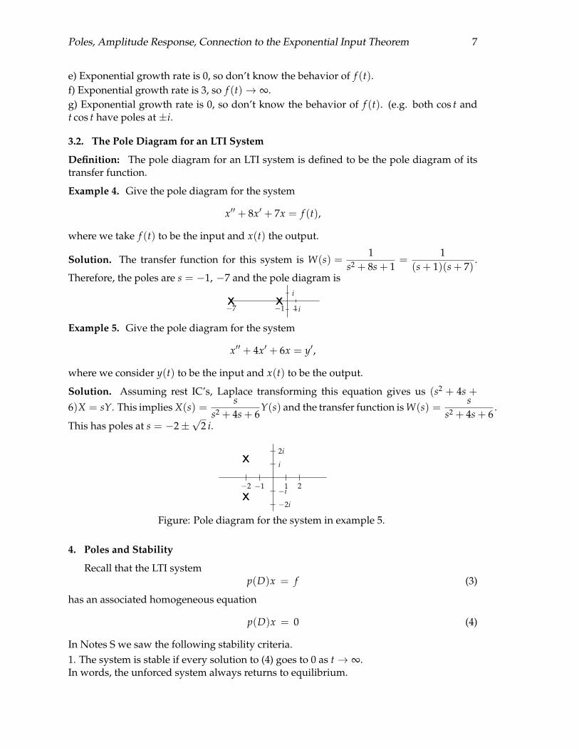
Poles, Amplitude Response, Connection to the Exponential Input Theorem 7
e) Exponential growth rate is 0, so don’t know the behavior of f (t).f) Exponential growth rate is 3, so f (t)→ ∞.g) Exponential growth rate is 0, so don’t know the behavior of f (t). (e.g. both cos t andt cos t have poles at ±i.
3.2. The Pole Diagram for an LTI System
Definition: The pole diagram for an LTI system is defined to be the pole diagram of itstransfer function.
Example 4. Give the pole diagram for the system
x′′ + 8x′ + 7x = f (t),
where we take f (t) to be the input and x(t) the output.
Solution. The transfer function for this system is W(s) =1
s2 + 8s + 1=
1(s + 1)(s + 7)
.
Therefore, the poles are s = −1, −7 and the pole diagram is
1−1−7
i
−iXX
Example 5. Give the pole diagram for the system
x′′ + 4x′ + 6x = y′,
where we consider y(t) to be the input and x(t) to be the output.
Solution. Assuming rest IC’s, Laplace transforming this equation gives us (s2 + 4s +6)X = sY. This implies X(s) =
ss2 + 4s + 6
Y(s) and the transfer function is W(s) =s
s2 + 4s + 6.
This has poles at s = −2±√
2 i.
1−1 2−2
i
−i
2i
−2i
X
X
Figure: Pole diagram for the system in example 5.
4. Poles and Stability
Recall that the LTI systemp(D)x = f (3)
has an associated homogeneous equation
p(D)x = 0 (4)
In Notes S we saw the following stability criteria.1. The system is stable if every solution to (4) goes to 0 as t→ ∞.In words, the unforced system always returns to equilibrium.

Poles, Amplitude Response, Connection to the Exponential Input Theorem 8
2. Equivalently, the system is stable if all the roots of the characteristic equation havenegative real part.
Now, since the transfer function for the system in (3) is1
p(s)the poles of the system are
just the characteristic roots. Comparing this with the stability criterion 2, gives us anotherway of expressing the stability criteria.
3. The system is stable if all its poles have negative real part.
4. Equivalently, the system is stable if all its poles lie strictly in the left half of the complexplane Re(s) < 0.
Criterion 4 tells us how to see at a glance if the system is stable, as illustrated in thefollowing example.
Example. Each of the following six graphs is the pole diagram of an LTI system. Say whichof the systems are stable.
(a)
1 3−1−3
i
3i
−i
−3i
XX
(b)
1 3−1−3
i
3i
−i
−3i
XX X
X
X
(c)
1 3−1−3
i
3i
−i
−3i
XXXX
(d)
1 3−1−3
i
3i
−i
−3i
XX X X
(e)
1 3−1−3
i
3i
−i
−3i
X
X
X
X
X
( f )
1 3−1−3
i
3i
−i
−3i
X
X
X
Solution. (a), (c) and (e) have all their poles in the left half-plane, so they are stable. Theothers do not, so they are not stable.
5. Poles and Amplitude Response
We started by considering the poles of functions F(s), and saw that, by definition, thegraph of |F(s)| went off to infinity at the poles. Since it tells us where |F(s)| is infinite,the pole diagram provides a crude graph of |F(s)|: roughly speaking, |F(s)| will be largefor values of s near the poles. In this note we show how this basic fact provides a usefulgraphical tool for spotting resonant or near-resonant frequencies for LTI systems.
Example 1. Figure 1 shows the pole diagram of a function F(s). At which of the points A,B, C on the diagram would you guess |F(s)| is largest?

Poles, Amplitude Response, Connection to the Exponential Input Theorem 9
1−1 2−2
i
−i
2i
−2i
X
X
X
X
•A
•B
•C
Figure 2: Pole diagram for example 1.
Solution. Point A is close to a pole and B and C are both far from poles so we would guesspoint |F(s)| is largest at point A.
Example 2. The pole diagram of a function F(s) is shown in Figure 2. At what point s onthe positive imaginary axis would you guess that |F(s)| is largest?
1−1 2−2
i
−i
2i
−2i
3i
−3i
X
X
X
X
X
Figure 2: Pole diagram for example 2.
Solution. We would guess that s should be close to 3 i, which is near a pole. There is notenough information in the pole diagram to determine the exact location of the maximum,but it is most likely to be near the pole.
5.1. Amplitude Response and the System Function
Consider the systemp(D)x = f (t). (5)
where we take f (t) to be the input and x(t) to be the output. The transfer function of thissystem is
W(s) =1
p(s). (6)
If f (t) = B cos(ωt) then equation FR (2) gives the following periodic solution to (5)
xp(t) =B cos(ωt− φ)
|p(iω)| , where φ = Arg(p(iω)). (7)
If the system is stable, then all solutions are asymptotic to the periodic solution in (7). In

Poles, Amplitude Response, Connection to the Exponential Input Theorem 10
this case, we saw (FR (3)) that the amplitude response of the system as a function of ω is
g(ω) =1
|p(iω)|. (8)
Comparing (6) and (8), we see that for a stable system the amplitude response is related tothe transfer function by
g(ω) = |W(iω)|. (9)
Note: The relation (9) holds for all stable LTI systems.
Using equation (9) and the language of amplitude response we will now re-do example2 to illustrate how to use the pole diagram to estimate the practical resonant frequencies ofa stable system.
Example 3. Figure 3 shows the pole diagram of a stable LTI system. At approximatelywhat frequency will the system have the biggest response?
1−1 2−2
i
−i
2i
−2i
3i
−3i
X
X
X
X
X
Figure 3: Pole diagram for example 3 (same as Figure 2).
Solution. Let the transfer function be W(s). Equation (9) says the amplitude responseg(ω) = |W(iω)|. Since iω is on the positive imaginary axis, the amplitude response g(ω)will be largest at the point iω on the imaginary axis where |W(iω)| is largest. This isexactly the point found in example 2. Thus, we choose iω ≈ 3i, i.e. the practical resonantfrequency is approximately ω = 3.
Note: Rephrasing this in graphical terms: we can graph the magnitude of the systemfunction |W(s)| as a surface over the s-plane. The amplitude response of the systemg(ω) = |W(iω)| is given by the part of the system function graph that lies above theimaginary axis. This is all illustrated beautifully by the applet Amplitude: Pole Diagram.

18.03 LA.1: Phase plane and linear systems
[1] Energy conservation[2] Energy loss[3] Companion system[4] Heat flow[5] Elimination
[1] Energy conservation
Let’s think again about the harmonic oscillator, mx + kx = 0. Thesolutions are sinusoids of angular frequency ω =
√k/m. The mass bounces
back and forth without damping. Let’s check conservation of energy.
From physics we know that energy is the sum of kinetic plus potential.Kinetic energy is given by
KE =mx2
2
Potential energy can be determined by computing work done. If we declarethe relaxed spring to have PE = 0, then using Hooke’s law when the mass isat position x
PE = −∫ x
0
−kx dx =kx2
2
(When you’re fighting the force, you increase potential energy, so the poten-tial energy is given by −
∫F dx. But the direction of force in Hooke’s law
opposes the displacement, so the force is −kx.)
So the total energy of the spring system is given by
E =kx2
2+
mx2
2(1)
Let’s see how it changes with time:
E = kxx + mxx = x(kx + mx) = 0
Conservation of energy is in force!
Energy is a function of two variables, x and x. The plane with thesecoordinates is called the phase plane. It is traditional to draw x horizontally
1

and x vertically. Contours of constant energy are curves on this plane, namelyellipses. Rearranging (1),
x2
2E/k+
x2
2E/m= 1
so the maximal value (i.e. the amplitude) of x is√
2E/k and the amplitude
of x is√
2E/m. These are the semi-axes of the ellipse. These formulas makesense: For given energy, small spring constant means big swing; small massmeans large velocity.
As time increases, the point (x(t), x(t)) traces out this ellipse. Which el-lipse depends on the energy. You get a whole family of nested non-intersectingcurves. This is called the phase diagram of this system.
Question 10.1. In which direction is the ellipse traversed?
1. Clockwise2. Counterclockwise3. Depends4. I don’t know
Well, above the axis x > 0, which means that x is increasing. So theanswer is 1, clockwise.
In a phase diagram, trajectories move to the right above the horizontalaxis, and to the left below it.
How about when the trajectory crosses the horizontal? Well there x = 0:the tangent is vertical. It crosses at right angles.
As the point moves around the ellipse, energy in the system sloshes backand forth between potential (when |x| is large and |x| is small) and kinetic(when |x| is large and |x| is small).
[2] Energy loss
What happens when we introduce some damping? So now
mx + bx + kx = 0 (2)
Our equation for the energy is unchanged, but now
E = x(kx + mx) = −bx2
2

Energy is lost to friction. The dashpot heats up. The loss is largest when |x|is largest, and zero when x = 0.
The effect of the friction is that the trajectory crosses through the equal-energy ellipses; it spirals in towards the origin, clockwise.
The x and x graphs are damped sinusoids, out of phase with each other.
Wait, that’s just the underdamped case. The other option is that thetrajectory just curves in to zero without spiralling. These are clearly shownin the Mathlet “Linear Phase Portraits: Matrix Entry.”
[3] The companion system
In introducing x as an independent variable, we’ve done something im-portant. We’ve rewritten the original equation as a first order equation. Tobe clear about this, let’s write y for the new variable. It’s related to x: y = x.What’s y? To keep the notation clean, let me replace b by b
mand k by k
m.
y = x = −kx− bx = −kx− by
So we have a pair of linked differential equations, a system of ordinary dif-ferential equations. (Sorry about the overuse of the word “system.”){
x = yy = −kx− by
This is called the companion system of the equation (2).
We might as well use vector notation:
u =
[xy
]so u =
[xy
]so we can write our equation using matrix multiplication:
u =
[0 1−k −b
]u
The matrix here is the companion matrix of the differential operator D2 +bD + kI.
This is pretty amazing! We have replaced a second order equation witha first order (but now vector-valued) equation!
3

You can even incorporate a forcing term:
x + bx + kx = q(t)
translates as {x = yy = −kx− by + q(t)
or
u =
[0 1−k −b
]u +
[0
q(t)
]Note also that the linear second order equation translated into a linear
first order vector valued equation, and that homogeneity is preserved.
You can do this with higher order equations too: For a third order equa-tion
...x + a2x + a1x + a0x = 0, say y = x, z = y, so z = −a2z − a1y − a0x
and
d
dt
xyz
=
0 1 00 0 1−a0 −a1 −a2
xyz
Side note: Numerical schemes work with first order equations only. To
solve a higher order equation numerically, one replaces it by its companionfirst order system. We’ll discuss this in December.
[4] Heat flow
Suppose I have a thermally insulated rod, and I’m interested in how heatflows through it.
I’ll install a thermometer every foot, and just think about heat transfersbetween those points. Suppose for a start that the rod is three feet long. Sothere are four temperatures, x0, x1, x2, and x3, to consider.
Let’s suppose that the temperatures at the end are fixed, constant, butx1 and x2 are functions of time.
Well, the linear or Newtonian approach goes as follows: if x0 > x1, therewill be an upward pressure on x1 that is proportional to the difference x0−x1.Independently of this, if x2 > x1, there will be an upward pressure on x1 thatis proportional to the difference x2 − x1.
Putting them together,
x1 = k((x0 − x1) + (x2 − x1)) = k(x0 − 2x1 + x2)
4

Similarly,x2 = k(x1 − 2x2 + x3)
This is a linked system of equations, which we can express in matrix form,using
d
dt
[x1
x2
]= k
[−2 11 −2
][x1
x2
]+ k
[x0
x3
](3)
A four foot section would lead to
d
dt
x1
x2
x3
= k
−2 1 01 −2 10 1 −2
x1
x2
x3
+ k
x0
0x4
and you can imagine from this what longer sections would look like.
The general picture is this: We have a system whose state is determinednot by a single number but rather by a vector u of n numbers. (Maybe
the vector is
[xx
], but maybe not.) The rate of change of u at time t
is determined by the value of u(t) (and perhaps the value of t), and wewill mainly assume that this determination is linear, which means that theequation is
u = Au + q(t)
where A is an n×n matrix A. The matrix A represents the physical system.q(t) is a “driving term” (perhaps the end point temperatures of the rod).To get a particular solution one has to specify an initial condition, u(0),consisting of n numbers.
There is a slight change of convention in force here: We are now isolatingthe u on the left, and putting everything else—representation of the systemand input signal alike—on the right. There’s a sign reversal that happens;this is reflected in the signs in the formula for the companion matrix.
First order systems of linear equations incorporate higher order lineardifferential equations, while giving natural representations of other types ofphysical phenomena. To gain the deepest possible insight into their behavior,it’s best to develop some of the theory of matrices, especially the squarematrices that show up in the model above.
5

[5] Elimination
Do you think we can rewrite the equation (3) as a second order equation?Let’s try. Maybe I’ll take x0 = x3 = 0, the homogeneous case. If we succeed:
Question 10.2 Do you expect this to be underdamped or overdamped?
1. Underdamped2. Overdamped
Well, do you really expect oscillations in the heat distribution? Let’s see.{x1 = −2kx1 + kx2
x2 = kx1 − 2kx2
Let’s try to eliminate x2. I can use the first equation to solve for it in termsof x1: kx2 = x1 + 2kx1. If I substitute this into k times the second equationI get
x1 + 2kx1 = k2x1 − 2k(x1 + 2kx1)
orx1 + 4kx1 + 3k2x1 = 0
OK, the characteristic polynomial is
p(s) = s2 + 4ks + 3k2 = (s + k)(s + k)
so the roots are −1 and −3. Overdamped. General solution:
x1 = ae−kt + be−3kt
You can always do this; but it’s not very systematic or insightful, and itbreaks the symmetry of the variables. Linear algebra offers a better way.
6

18.03 LA.2: Matrix multiplication, rank, solving linearsystems
[1] Matrix Vector Multiplication Ax[2] When is Ax = b Solvable ?[3] Reduced Row Echelon Form and Rank[4] Matrix Multiplication[5] Key Connection to Differential Equations
[1]Matrix Vector Multiplication Ax
Example 1:
Ax =
1 24 53 7
[x1
x2
].
I like to think of this multiplication as a linear combination of the columns:
Ax =
1 24 53 7
[x1
x2
]= x1
143
+ x2
257
.
Many people think about taking the dot product of the rows. That isalso a perfectly valid way to multiply. But this column picture is very nicebecause it gets right to the heart of the two fundamental operation that wecan do with vectors.
We can multiply them by scalar numbers, such as x1 and x2, and we canadd vectors together. This is linearity.
[2] When is Ax = b Solvable?
There are two main components to linear algebra:
1. Solving an equation Ax = b
2. Eigenvalues and Eigenvectors
This week we will focus on this first part. Next week we will focus on thesecond part.
1

Given an equation Ax = b, the first questions we ask are :
Question Is there a solution?
Question If there is a solution, how many solutions are there?
Question What is the solution?
Example 2: Let’s start with the first question. Is there a solution to thisequation? 1 2
4 53 7
[x1
x2
]=
b1b2b3
3× 2 2× 1 3× 1
Notice the dimensions or shapes. The number of columns of A must beequal to the number of rows of x to do the multiplication, and the vectorwe get has the dimension with the same number of rows as A and the samenumber of columns as x.
Solving this equation is equivalent to finding x1 and x1 such that thelinear combination of columns of A gives the vector b.
Example 3: 1 24 53 7
[x1
x2
]=
257
The vector b is the same as the 2nd column of A, so we can find this solution
by inspection, the answer is x =
[01
].
But notice that this more general linear equation from Example 2:1 24 53 7
[x1
x2
]=
b1b2b3
is a system with 3 equations and 2 unknowns. This most likely doesn’t have asolution! This would be like trying to fit 3 points of data with a line. Maybeyou can, but most likely you can’t!
To understand when this system has a solution, let’s draw a picture.
2

All linear combinations of columns of A lie on a plane.
What are all linear combinations of these two columns vectors? How doyou describe it?
It’s a plane! And it is a plane that goes through the origin, because
0
143
+ 0
257
= 0.
It is helpful to see the geometric picture in these small cases, because thegoal of linear algebra is to deal with very large matrices, like 1000 by 100.(That’s actually a pretty small matrix.)
What would the picture of a 1000 by 100 matrix be?
It lives in 1000-dimensional space. What would the 100 column vectorsspan? Or, what is the space of all possible solutions?
Just a hyperplane, a flat, thin, at most 100-dimensional space inside of1000-dimensions. But linear algebra gets it right! That is the power of linear
3

algebra, and we can use our intuition in lower dimensions to do math onmuch larger data sets.
The picture exactly tells us what are the possible right hand sides tothe equation. Ax = b/ If b is in the plane, then there is a solution to theequation!
All possible b ⇐⇒ all possible combinations Ax.
In our case, this was a plane. We will call this plane, this subspace, thecolumn space of the matrix A.
If b is not on that plane, not in that column space, then there is nosolution.
Example 4: What do you notice about the columns of the matrix in thisequation? 1 3
4 123 9
[x1
x2
]=
b1b2b3
The 2nd column is a multiple of the 1st column. We might say these
columns are dependent.
The picture of the column space in this case is a line.
All linear combinations of columns of A lie along a line.
4

[3] Reduced Row Echelon Form and Rank
You learned about reduced row echelon form in recitation. Matlab andother learn algebra systems do these operation.
Example 5: Find the reduced row echelon form of our matrix:1 24 53 7
.
It is 1 00 10 0
.
It is very obvious that the reduced row echelon form of the matrix has 2columns that are independent.
Let’s introduce a new term the rank of a matrix.
Rank of A = the number of independent columns of A.
Example 6: Find the row echelon form of1 34 123 9
.
But what do you notice about the rows of this matrix? We made thismatrix by making the columns dependent. So the rank is 1. We didn’t touchthe rows, this just happened.
How many independent rows are there?
1!
The reduced row echelon form of this matrix is1 30 00 0
?
5

This suggests that we can define rank equally well as the number ofindependent rows of A.
Rank of A = the number of independent columns of Athe number of independent rows of A
The process of row reduction provides the algebra, the mechanical stepsthat make it obvious that the matrix in example 5 has rank 2! The steps ofrow reduction don’t change the rank, because they don’t change the numberof independent rows!
Example 7: What if I create a 7x7 matrix with random entries. How manylinearly independent columns does it have?
7 if it is random!
What is the row echelon form? It’s the identity.
To create a random 7x7 matrix with entries random numbers between 0and 1, we write
rand(7).
The command for reduced row echelon form is rref. So what you will see isthat
rref(rand(7))=eye(7).
The command for the identity matrix is
eye(n).
That’s a little Matlab joke.
[4] Matrix Multiplication
We thought of Ax = b as a combination of columns. We can do the samething with matrix multiplication.
AB = A
| | |b1 b2 · · · bn
| | |
=
| | |Ab1 Ab2 · · · Abn
| | |
6

This perspective leads to a rule A(BC) = (AB)C. This seemingly simplerule takes some messing around to see. But this observation is key to manyideas in linear algebra. Note that in general AB 6= BA.
[5] Key Connection to Differential Equations
We want to find solutions to equations Ax = b where x is an unknown.
You’ve seen how to solve differential equations like
dx
dt− 3t5x = b(t).
The key property of this differential equation is that it is linear in x. To finda complete solution we need to find one particular solution and add to it allthe homogeneous solution. This complete solution describes all solutions tothe differential equation.
The same is true in linear algebra! Solutions behave the same way. Thisis a consequence of linearity.
Example: 8 Let’s solve 1 34 123 9
[x1
x2
]=
286
.
This matrix has rank 1, it has dependent columns. We chose b so thatthis equation is solvable. What is one particular solution?
xp =
[20
]is one solution. There are many solutions. For example[
−11
] [5−1
] [−22
8
]But we only need to choose one particular solution. And we’ll choose [2;0].
What’s the homogeneous solution? We need to solve the equation1 34 123 9
[x1
x2
]=
000
.
7

One solution is
[−31
], and all solutions are given by scalar multiples of
this one solution, so all homogenous solutions are described by
xh = c
[−31
]c a real number.
The complete solution is
xcomplete =
[20
]+ c
[−31
].
Here is how linearity comes into play!
Axcomplete = A(xp + xh) = Axp + Axh =
b1b2b3
+
000
8

18.03 LA.3: Complete Solutions, Nullspace, Space,Dimension, Basis
[1] Particular solutions[2] Complete Solutions[3] The Nullspace[4] Space, Basis, Dimension
[1] Particular solutions
Matrix Example
Consider the matrix equation
[1 1
] [x1
x2
]=[8]
The complete solution to this equation is the line x1 + x2 = 8. Thehomogeneous solution, or the nullspace is the set of solutions x1 + x2 = 0.This is all of the points on the line through the origin. The homogeneousand complete solutions are picture in the figure below.
Figure 1: The homogeneous and complete solutions
1

To describe a complete solution it suffices to choose one particular solu-tion, and add to it, any homogeneous solution. For our particular solution,we might choose [
80
]or
[08
]or
[44
]If we add any homogeneous solution to this particular solution, you move
along the line x1 +x2 = 8. All this equation does is take the equation for thehomogeneous line, and move the origin of that line to the particular solution!
How do solve this equation in Matlab? We type
x = [1 1] \ [8]
In general we write
x = A \ b
Differential Equations Example
Let’s consider the linear differential equation with initial condition given:
dy
dt+ y = 1
y(0)
To solve this equation, we can find one particular solution and add toit any homogeneous solution. The homogeneous solution that satisfies theinitial condition is xh = y(0)e−t. So then a particular solution must satisfyyp(0) = 0 so that xp(0) + xh(0) = y(0), and such a particular solution isyp = 1− e−t. The complete solution is then:
complete solution particular solution homogeneous solutiony = 1− e−t + y(0)e−t
However, maybe you prefer to take the steady state solution. The steadystate solution is when the derivative term vanishes, dy
dt= 0. So instead we
2

can choose the particular solution yp = 1. That’s an excellent solution tochoose. Then in order to add to this an homogeneous solution, we add somemultiple of e−t so that at t = 0 the complete solution is equal to y(0) and wefind
complete solution particular solution homogeneous solution
y = 1 + (y(0)− 1)e−t
↑ ↑steady state solution transient solution
The solution 1 is an important solution, because all solutions, no matterwhat initial condition, will approach the steady state solution y = 1.
There is not only 1 particular solution. There are many, but we have tochoose 1 and live with it. But any particular solution will do.
[2] Complete Solutions
Matrix Example
Let’s solve the system:
x1 +cx3 = b1x2 +dx3 = b2
What is the matrix for this system of equations?
A =
[1 0 c0 1 d
]Notice that A is already in row echelon form! But we could start with
any system
x1 +3x2 +5x3 = b14x1 +7x2 +19x3 = b2
3

and first do a sequence of row operations to obtain a row echelon matrix.(Don’t forget to do the same operations to b1 and b2:[
2 3 5... b1
4 7 17... b2
]−→
[2 3 5
... b1
0 1 9... b2 − 2b1
]−→
[1 3/2 5/2
... b1/2
0 1 9... b2 − 2b1
]
−→
[1 0 −11
... 5b1/2− 3b2/2
0 1 9... b2 − 2b1
]
Let’s find the complete solution to Ax = b for the matrix
A =
[1 0 c0 1 d
].
Geometrically, what are we talking about?
The solution to each equation is a plane, and the planes intersect in a line.That line is the complete solution. It doesn’t go through 0! Only solutionsto the equation Ax = 0 will go through 0!
So let’s find 1 particular solution, and all homogeneous solutions.
Recommended particular solution: Set the free variable x3 = 0. Then
xp =
b1b20
.
We could let the free variable be any value, but 0 is a nice choice becausewith a reduced echelon matrix, it is easy to read off the solution.
So what about the homogenous, or null solution. I will write xn insteadof xh for the null solution of a linear system, but this is the same as thehomogeneous solution. So now we are solving Ax = 0. The only bad choiceis x3 = 0, since that is the zero solution, which we already know. So insteadwe choose x3 = 1. We get
xn = C
−c−d1
4

The complete solution is
xcomplete =
b1b20
+ C
−c−d1
.
This is the power of the row reduced echelon form. Once in this form,you can read everything off!
Differential Equations Example
Let’s consider the differential equation y′′+ y = 1. We can choose the steadystate solution for the particular solution yp = 1.
Let’s focus on solving y′′+ y = 0. What is the nullspace of this equation?
We can’t say vectors here. We have to say functions. But that’s OK.We can add functions and we can multiply them by constants. That’s all wecould do with vectors too. Linear combinations are the key.
So what are the homogeneous solutions to this equation? Give me justenough, but not too many.
One answer is yh = c1 cos(t) + c2 sin(t). Using linear algebra terminology,I would say there is a 2-dimensional nullspace. There are two independentsolutions cos(t) and sin(t), and linear combinations of these two solutionsgives all solutions!
sin(t) and cos(t) are a basis for the nullspace.
A basis means each element of the basis is a solution to Ax = 0. Canmultiply by a constant and we still get a solution. And we can add togetherand still get a solution. Together we get all solutions, but the sin(t) andcos(t) are different or indepenedent solutions.
What’s another description of the nullspace?
C1eit + C2e
−it
This description is just as good. Better in some ways (fulfills the patternbetter), not as good in others (involves complex numers). The basis in thiscase is eit and e−it. They are independent solutions, but linear combinationsgive all null solutions.
5

If you wanted to mess with your TA, you could choose yh = Ceit+D cos(t).This is just as good.
We’ve introduced some important words. The basis for the nullspace. Inthis example, the beauty is that the nullspace will always have 2 functionsin it. 2 is a very important number.
• The degree of the ODE is 2
• There are 2 constants
• 2 initial conditions are needed
• The dimension of the nullspace is 2.
[3] The nullspace
Suppose we have the equation Rx = 0. The collection of x that solve thisequation form the nullspace. The nullspace always goes through the origin.
Example
Suppose we have a 5 by 5 matrix. Does it have an inverse or doesn’t it?Look at the nullspace! If only solution in the nullspace is 0, then yes, it isinvertible. However, if there is some nonzero solution, then the matrix is notinvertible.
The other importan work we used is space.
Matrix Example
Let NR denote the nullspace of R:
R =
[1 0 c0 1 d
]
What’s a basis for the nullspace? A basis could be
−c−d1
. Or we could
6

take
−2c−2d
2
. The dimension is 3 − 2 = 1. So there is only one element in
the basis.
Why can’t we take 2 vectors in the basis?
Because they won’t be independent elements!
Differential Equations Example
For example, Ceit + D cos(t) + E sin(t) does not form a basis because theyare not independent! Euler’s formula tells us that eit = cos(t) + i sin(t), soeit depends on cos(t) and sin(t).
[4] Space, Basis, Dimension There are a lot of important words that havebeen introduced.
• Space
• Basis for a Space
• Dimension of a Space
We have been looking at small sized examples, but these ideas are notsmall, they are very central to what we are studying.
First let’s consider the word space. We have two main examples. Thecolumn space and the nullspace.
A Column Space NullspaceDefinition All linear cominations of the columns of A All solutions to Ax = 0
50× 70 matrix Column space lives in R50 Nullspace lives in R70
m× n matrix Column space lives in Rm Nullspace lives in Rn
Definition V is a space (or vector space) when: if x and y are in thespace, then for any constant c, cx is in the space, and x + y is also in thespace. That’s superposition!
Let’s make sense of these terms for a larger matrix that is in row echelonform.
7

Larger Matrix Example
R =
= 1 2 0 30 0 1 40 0 0 0
.
The first and third columns are the pivot columns. The second and forthare free columns.
What is the column space, C(R)?
All linear combinations of the columns. Is
333
in the column space? No
it’s not. The column space is the xy-plane, all vectors
ab0
. The dimension
is 2, and a basis for the column space can be taken to be the pivot columns.1
00
,
010
Note, if your original matrix wasn’t in rref form, you must take the orig-
inal form of the pivot columns as your basis, not the row reduced form ofthem!
What is a basis for the nullspace, N(R)?−2100
,
−3041
The reduced echelon form makes explicit the linear relations between thecolumns.
The relationships between the columns of A are the same as the linearrelationships between the columns of any row-equivalent matrix, such as thereduced echelon form R. So a pivot indicates that this column is independentof the previous columns; and, for example, the 2 in the second column in this
8

reduced form is a record of the fact that the second column is 2 times thefirst. This is why the reduced row echelon form is so useful to us. It allowsus to immediately read off a basis for both the independent columns, andthe nullspace.
Note that this line of thought is how you see that the reduced echelonform is well-defined, independent of the sequence of row operations used toobtain it.
9

18.03 LA.4: Inverses and Determinants
[1] Transposes[2] Inverses[3] Determinants
[1] Transposes
The transpose of a matrix A is denoted AT , or in Matlab, A′.
The transpose of a matrix exchanges the rows and columns. The ithcolumn becomes the ith row. Or the aij entry becomes the aji entry.
Example:
A =
[1 2 43 5 7
] 1 32 54 7
Symmetric Matrices are square matrices that satisfy A = AT .
Example:
A =
1 3 93 2 59 5 8
We’ll see that the eigenvalues of symmetric matrices are great. The eigen-
vectors are even better! And symmetric matrices come up all of the time.
Property of transposes:
(AB)T = BTAT
1

[2] Inverses
Important questions:
• Is a matrix A invertible?
• How do you compute the inverse?
Let A be a square matrix. Suppose it has an inverse. We denote theinverse by A−1, and it has the property that
AA−1 = I A−1A = I.
The fact that the inverse is simultaneously a right and left inverse is notimmediately obvious. See if you can use the associative property (AB)C =A(BC) to see why this must be the case when A is square.
If the inverse of A and B both exists, and both matrices have the sameshape, then
(AB)−1 = B−1A−1
Corny Example:
If B represents taking off your jacket, and A represents taking off yoursweater, then it makes sense that you first take of your jacket, and thentake off your sweater. To find the inverse, which is to reverse this process,it makes sense that we have to reverse the order. First you put the sweaterback on, and then you put your jacket on.
So let’s start to answer our question: when is a matrix invertible? Toanswer this question, we’ll look at when it is NOT invertible first.
A is NOT invertible when:
• The determinant of A is zero.
• There exists a nonzero vector x so that Ax = 0.
2

Examples of matrices that are easy to invert:
2 by 2 matrices are easy to invert:[a bc d
]−1=
1
ad− bc
[d −bc a
]Check that the product of this matrix with its inverse is the identity.
The quantity in the denominator ad−bc is the determinant of that matrix.That’s why it can’t be zero. This is true for 5 by 5 matrices, 10 by 10 matrices,the inverse will always involve dividing by the determinant.
Diagonal matrices are easy to invert:
d1
d2d3
d4
−1
=
1/d1
1/d21/d3
1/d4
Example of non-invertible matrix
A =
3 −1 −2−4 7 −3−3 −2 5
We notices that the sum of each row is zero. So
3 −1 −2−4 7 −3−3 −2 5
1111
= 0
The vector[1 1 1 1
]Tis in the nullspace of A.
Let’s see why if there is a nonzero vector in the nullspace, then A can’tbe invertible.
3

Proof: Suppose x 6= 0 and Ax = 0. If A−1 existed, then
A−1Ax = A−10
Ix = 0
x = 0
This contradiction forces us to accept that an inverse must not exist!QED
Conditions for Invertibility:
• detA 6= 0.
• Nullspace of A is 0.
• Columns are independent.
• A has full rank (rank of A = n if A is an n by n matrix).
• Rows are independent.
• The row echelon form of A has a full set of nonzero pivots.
• rref A is the identify.
• Ax = b has a solution for every b.
This last condition is the question we’ve been interested in, when canwe solve this equation. The idea is that when it is always solvable, thenx = A−1b.
Proof:
Ax = b
A−1Ax = A−1b
x = A−1b
QED
4

Triangular Matrices
If A is upper triangular,
A =
∗ ∗ ∗ ∗0 ∗ ∗ ∗0 0 ∗ ∗0 0 0 ∗
we can tell whether or not A is invertible immediately by looking at thediagonal, or pivot entries. If all the diagonal entries are nonzero, the matrixis invertible.
For example, the matrix 3 π e ρ0 2 δ 00 0 1 00 0 0 7
is invertible, and its determinant is the product of these pivots, which is 42.
Computing Inverses
We’ve seen a bunch of connected ideas about when a matrix is invertible.And it is important to understand that you basically never want to computethe inverse. In Matlab, you could solve the equation Ax = b by typing
inv(A)*b
This is correct, but not smart. Instead, use
A \ b
which cleverly checks for certain forms of a matrix, and ultimately will rowreduce to find the solution.
However, if we want to compute A−1 there is a complicated formula in-volving determinants. But what you want to do is really solve the equation
5
AA−1 = I. Let a′1, a′2, . . . , a
′n denote the columns of A−1. Then solving for
A−1 is equivalent to solving the n equations:
Aa′1 =
100...0
Aa′2 =
010...0
· · · Aa′n =
00...01
Recall that to solve Ax = b, we augment the matrix A with the column
b and do row operations until we end up with a row reduced matrix wherewe can read off the solutions:
[A|b] −→ Apply row operations −→ [R|d]
It turns out we can solve all n of our equations simulaneously by aug-menting the matrix A with the matrix I, [A|I] and then performing rowoperations. Because A is invertible, its reduced row echelon form is I, andwhat you end up with is I on the left, augmented by the solutions to Ax = Ion the right. But that solution is exactly A−1.
Computing the inverse
• Augment A with the identity matrix: [A|I]
• Apply row operations until A reaches row reduced echelon form (rref)
• What you are left with on the augmented side is the collection ofcolumns of A−1: [I|A−1]
[3] Determinants
Example 2 by 2
det
[a bc d
]= ad− bc
6

In general, the determinant of a square matrix is a single number. Thisentry depends on all of the entries of the matrix.
Properties of the determinant:
• det I = 1
• If you subtract m times row i and subtract that from row j, the de-terminants is unchanged! Example, subtract 4 times row 1 from row2:
det
1 1 14 3 17 2 1
= det
1 1 10 −1 −37 2 1
• If you exchange rows, the determinant changes sign. Example:
det I = − det
1 0 00 0 10 1 0
• If you multiply a row by a number c, the determinant is multiplied byc.
det
c c c4 3 17 2 1
= c det
1 1 14 3 17 2 1
• det(AB) = detA detB
Example
Suppose I have a matrix A such that two of its rows are equal. Then if Iexchange those rows, the matrix is unchanged. But by the third property,this implies that detA = − detA, which can only be true if detA is zero. Thistells us that any matrix whose rows and not independent has determinantequal to zero.
7

Example 3 by 3
The 3 by 3 determinant has 6 = 3! terms. Each term is a multiple of a threeentries, one from each row and column.
1 2 32 3 43 4 5
= 1 · 3 · 5 + 2 · 4 · 3 + 3 · 2 · 4− 2 · 2 · 5− 1 · 4 · 4− 3 · 3 · 3
This matrix satisfies the equation1 2 32 3 43 4 5
−12−1
=
000
so the determinant must be zero.
In general, the determinant of an n by n matrix is a sum of n! terms allcombined into one number. A 4 by 4 matrix already has 24 terms! Thatis a lot of terms. The key idea here is that if a matrix is not invertible, itsdeterminant is zero.
8

18.03 LA.5: Eigenvalues and Eigenvectors
[1] Eigenvectors and Eigenvalues[2] Observations about Eigenvalues[3] Complete Solution to system of ODEs[4] Computing Eigenvectors[5] Computing Eigenvalues
[1] Eigenvectors and Eigenvalues
Example from Differential Equations
Consider the system of first order, linear ODEs.
dy1dt
= 5y1 + 2y2
dy2dt
= 2y1 + 5y2
We can write this using the companion matrix form:[y′1y′2
]=
[5 22 5
] [y1y2
].
Note that this matrix is symmetric. Using notation from linear algebra,we can write this even more succinctly as
y′ = Ay.
This is a coupled equation, and we want to uncouple it.
Method of Optimism
We’ve seen that solutions to linear ODEs have the form ert. So we will lookfor solutions
1

y1 = eλta
y2 = eλtb
Writing in vector notation:
y = eλt[ab
]= eλtx
Here λ is the eigenvalue and x is the eigenvector.
To find a solution of this form, we simply plug in this solution into theequation y′ = Ay:
d
dteλtx = λeλtx
Aeλtx = eλtAx
If there is a solution of this form, it satisfies this equation
λeλtx = eλtAx.
Note that because eλt is never zero, we can cancel it from both sides ofthis equation, and we end up with the central equation for eigenvalues andeigenvectors:
λx = Ax
Definitions
• A nonzero vector x is an eigenvector if there is a number λ such thatAx = λx.
• The scalar value λ is called the eigenvalue.
Note that it is always true that A0 = λ · 0 for any λ. This is why wemake the distinction than an eigenvector must be a nonzero vector, and aneigenvalue must correspond to a nonzero vector. However, the scalar valueλ can be any real or complex number, including 0.
2

This is a subtle equation. Both λ and x are unknown. This isn’t exactlya linear problem. There are more unknowns.
What is this equation saying? It says that we are looking for a vector xsuch that x and Ax point in the same direction. But the length can change,the length is scaled by λ.
Note that this isn’t true for most vectors. Typically Ax does not pointin the same direction as x.
Example
If λ = 0, our central equation becomes Ax = 0x = 0. The eigenvector xcorresponding to the eigenvalue 0 is a vector in the nullspace!
Example
Let’s find the eigenvalues and eigenvectors of our matrix from our system ofODEs. That is, we want to find x and λ such that[
5 22 5
] [??
]= λ
[??
]By inspection, we can see that[
5 22 5
] [11
]= 7
[11
].
We have found the eigenvector x1 =
[11
]corresponding to the eigenvalue
λ1 = 7.
So a solution to a differential equation looks like
y = e7t[11
]Check that this is a solution by pluging
y1 = e7t and
y2 = e7t
3

into the system of differential equations.
We can find another eigenvalue and eigenvector by noticing that[5 22 5
] [1−1
]= 3
[1−1
].
We’ve found the nonzero eigenvector x2 =
[1−1
]with corresponding
eigenvalue λ2 = 3.
Check that this also gives a solution by plugging
y1 = e3t and
y2 = −e3t
back into the differential equations.
Notice that we’ve found two independent solutions x1 and x2. More istrue, you can see that x1 is actually perpendicular to x2. This is becausethe matrix was symmetric. Symmetric matrices always have perpendiculareigenvectors.
[2] Observations about Eigenvalues
We can’t expect to be able to eyeball eigenvalues and eigenvectors everytime.Let’s make some useful observations.
We have
A =
[5 22 5
]and eigenvalues
λ1 = 7
λ2 = 3
• The sum of the eigenvalues λ1 + λ2 = 7 + 3 = 10 is equal to the sum ofthe diagonal entries of the matrix A is 5 + 5 = 10.
4

The sum of the diagonal entries of a matrix A is called the trace and isdenoted tr (A).
It is always true thatλ1 + λ2 = tr (A).
If A is an n by n matrix with n eigenvalues λ1, . . . , λn, then
λ1 + λ2 + · · ·+ λn = tr (A)
• The product of the eigenvalues λ1λ2 = 7 · 3 = 21 is equal to detA =25− 4 = 21.
In fact, it is always true that
λ1 · λ2 · · ·λn = detA .
For a 2 by 2 matrix, these two pieces of information are enough to computethe eigenvalues. For a 3 by 3 matrix, we need a 3rd fact which is a bit morecomplicated, and we won’t be using it.
[3] Complete Solution to system of ODEs
Returning to our system of ODEs:[y′1y′2
]=
[5 22 5
] [y1y2
].
We see that we’ve found 2 solutions to this homogeneous system.[y1y2
]= e7t
[11
]and e3t
[1−1
]The general solution is obtained by taking linear combinations of these
two solutions, and we obtain the general solution of the form:[y1y2
]= c1e
7t
[11
]+ c2e
3t
[1−1
]5

The complete solution for any system of two first order ODEs has the form:
y = c1eλ1tx1 + c2e
λ2tx2,
where c1 and c2 are constant parameters that can be determined from theinitial conditions y1(0) and y2(0). It makes sense to multiply by this param-eter because when we have an eigenvector, we actually have an entire line ofeigenvectors. And this line of eigenvectors gives us a line of solutions. Thisis what we’re looking for.
Note that this is the general solution to the homogeneous equation y′ =Ay. We will also be interested in finding particular solutions y′ = Ay + q.But this isn’t where we start. We’ll get there eventually.
Keep in mind that we know that all linear ODEs have solutions of theform ert where r can be complex, so this method has actually allowed us tofind all solutions. There can be no more and no less than 2 independentsolutions of this form to this system of ODEs.
In this example, our matrix was symmetric.
• Symmetric matrices have real eigenvalues.
• Symmetric matrices have perpendicular eigenvectors.
[4] Computing Eigenvectors
Let’s return to the equation Ax = λx.
Let’s look at another example.
Example
A =
[2 40 3
]This is a 2 by 2 matrix, so we know that
λ1 + λ2 = tr (A) = 5
λ1 · λ2 = det(A) = 6
6

The eigenvalues are λ1 = 2 and λ2 = 3. In fact, because this matrix wasupper triangular, the eigenvalues are on the diagonal!
But we need a method to compute eigenvectors. So lets’ solve
Ax = 2x.
This is back to last week, solving a system of linear equations. The key ideahere is to rewrite this equation in the following way:
(A− 2I)x = 0
How do I find x? I am looking for x in the nullspace of A− 2I! And wealready know how to do this.
We’ve reduced the problem of finding eigenvectors to a problem that wealready know how to solve. Assuming that we can find the eigenvalues λi,finding xi has been reduced to finding the nullspace N(A− λiI).
And we know that A − λI is singular. So let’s compute the eigenvectorx1 corresponding to eigenvalue 2.
A− 2I =
[0 40 1
]x1 =
[00
]By looking at the first row, we see that
x1 =
[10
]is a solution. We check that this works by looking at the second row.
Thus we’ve found the eigenvector x1 =
[10
]corresponding to eigenvalue
λ1 = 2.
Let’s find the eigenvector x2 corresponding to eigenvalue λ2 = 3. We dothis by finding the nullspace N(A− 3I), we wee see is
A− 3I =
[−1 40 0
] [41
]=
[00
]
The second eigenvector is x2 =
[41
]corresponding to eigenvalue λ2 = 3.
7

Important observation: this matrix is NOT symmetric, and the eigenvec-tors are NOT perpendicular!
[5] Method for finding Eigenvalues
Now we need a general method to find eigenvalues. The problem is to find λin the equation Ax = λx.
The approach is the same:
(A− λI)x = 0.
Now I know that (A−λI) is singular, and singular matrices have determi-nant 0! This is a key point in LA.4. To find λ, I want to solve det(A−λI) = 0.The beauty of this equation is that x is completely out of the picture!
Consider a general 2 by 2 matrix A:
A =
[a bc d
]A− λI =
[a− λ bc d− λ
].
The determinant is a polynomial in λ:
det(A− λI) = λ2 − (a+ d)λ + (ad− bc) = 0↑ ↑
tr (A) det(A)
This polynomial is called the characteristic polynomial. This polynomialis important because it encodes a lot of important information.
The determinant is a polynomial in λ of degree 2. If A was a 3 by 3matrix, we would see a polynomial of degree 3 in λ. In general, an n by nmatrix would have a corresponding nth degree polynomial.
Definition
The characteristic polynomial of an n by n matrix A is the nth degree poly-nomial det(A− λI).
8

• The roots of this polynomial are the eigenvalues of A.
• The constant term (the coefficient of λ0) is the determinant of A.
• The coefficient of λn−1 term is the trace of A.
• The other coefficients of this polynomial are more complicated invari-ants of the matrix A.
Note that it is not fun to try to solve polynomial equations by hand ifthe degree is larger than 2! I suggest enlisting some computer help.
But the fundamental theorem of arithmetic tells us that this polynomialalways has n roots. These roots can be real or complex.
Example of imaginary eigenvalues and eigenvectors[cos(θ) − sin(θ)sin(θ) cos(θ)
]Take θ = π/2 and we get the matrix
A =
[0 −11 0
].
What does this matrix do to vectors?
To get a sense for how this matrix acts on vectors, check out the MatrixVector Mathlet http://mathlets.org/daimp/MatrixVector.html
Set a = d = 0, b = −1 and c = 1. You see the input vector v in yellow,and the output vector Av in blue.
What happens when you change the radius? How is the magnitude of theoutput vector related to the magnitude of the input vector?
Leave the radius fixed, and look at what happens when you vary the angleof the input vector. What is the relationship between the direction of theinput vector and the direction of the output vector?
This matrix rotates vectors by 90 degrees! For this reason, there can beno real nonzero vector that points in the same direction after being multiplied
9

by the matrix A. Let’s look at the characteristic polynomial and find theeigenvalues.
det(A− λI) = det
[−λ −11 −λ
]= λ2 + 1 = 0
The eigenvalues are λ1 = i and λ2 = −i.Let’s do a quick check:
• λ1 + λ2 = i− i = tr (A)
• λ1 · λ2 = (i)(−i) = −1 = det(A)
Let’s find the eigenvector corresponding to eigenvalue i:
A− iI =
[−i −11 i
]Solving for the nullspace we must find the solution to the equation:[
−i −11 i
] [??
]=
[00
]To solve this equation, I look at the first row, and checking against the
second row we find that the solution is[−i −11 i
] [1−i
]=
[00
].
What ODE does this correspond to?[y′1y′2
]=
[−i −11 i
] [y1y2
]This is the system
y′1 = y2
y′2 = y1
10

Using the method of elimination we get that:
y′′1 = −y′2 = −y1
We are very familiar with this differential equation, it is the harmonicoscillator y′′ + y = 0. This linear, 2nd order equation parameterized motionaround a circle! It is a big example and physics, and we know that thesolution space has a basis spanned by eit and e−it. Notice that the i and −iare the eigenvalues!
Properties of Eigenvalues
Suppose A has eigenvalue λ and nonzero eigenvector x.
• The the eigenvalues of A2 are λ2.
Why?A2x = λAx = λ2x
We see that the vector x will also be an eigenvector corresponding to λ.However, be careful!!! In the example above, λ1 = i and λ2 = −1, we getrepeated eigenvalues λ1 = λ2 = −1. And in fact
[0 −11 0
]2=
[−1 00 −1
]= −I
Since −Ix = −x for all nonzero vectors x, in fact every vector in theplane is an eigenvector with eigenvalue -1!
We know that the exponential function is important.
• The eigenvalues of eA are eλ, with eigenvector x.
If eAx had meaning,eAx = eλx
where x is an eigenvector of A, and λ is the corresponding eigenvalue.
• The eigenvalues of e−1 are λ−1, with eigenvector x.
11
Let’s look at the example A =
[5 22 5
], which had eigenvalues 7 and 3. Check
that A−1 has eigenvalues 1/7 and 1/3. We know that det(A) ∗ det(A−1) = 1,and det(A) = 21 and det(A−1) = 1/21, which is good.
• The eigenvalues of A+ 12I are λ+ 12, with eigenvector x.
Check this with our favorite symmetric matrix A above.
Nonexamples
Let A and B be n by n matrices.
• The eigenvalues of A+B are generally NOT the eigenvalues of A pluseigenvalues of B.
• The eigenvalues of AB are generally NOT the eigenvalues of A timesthe eigenvalues of B.
Question: What would be necessary for the eigenvalues of A+B to be thesum of the eigenvalues of A and B? Similarly for AB.
Keep in mind that Ax = λx is NOT an easy equation.
In matlab, the command is
eig(A)
12

18.03 LA.6: Diagonalization and Orthogonal Matrices
[1] Diagonal factorization[2] Solving systems of first order differential equations[3] Symmetric and Orthonormal Matrices
[1] Diagonal factorization
Recall: if Ax = λx, then the system y = Ay has a general solution of theform
y = c1eλ1tx1 + c2e
λ2tx2,
where the λi are eigenvalues with corresponding eigenvectors xi.
I’m never going to see eigenvectors without putting them into a matrix.And I’m never going to see eigenvalues without putting them into a matrix.Let’s look at an example from last class.
A =
[5 22 5
]. We found that this had eigenvectors
[11
]and
[1−1
].
I’m going to form a matrix out of these eigenvectors called the eigenvectormatrix S:
S =
[1 11 −1
]Then lets look at what happens when we multiply AS, and see that we
can factor this into S and a diagonal matrix Λ:[5 22 5
] [1 11 −1
]=
[7 37 −3
]=
[1 11 −1
] [7 00 3
]A S S Λ
We call matrix Λ with eigenvalues λ on the diagonal the eigenvalue matrix.
So we see that AS = SΛ, but we can multiply both sides on the right byS−1 and we get a factorization A = SΛS−1. We’ve factored A into 3 pieces.
1

Properties of Diagonalization
• A2 = SΛS−1SΛS−1 = SΛ2S−1
• A−1 = (SΛS−1)−1 = (S−1)−1Λ−1S−1 = SΛ−1S−1
Diagonal matrices are easy to square and invert because you simply squareor invert the elements along the diagonal!
[2] Solving systems of first order differential
equations
The entire reason we are finding eigenvectors is to solve differential equations.Let’s express our solution to the differential equation in terms of S and Λ:
y =[x1 x2
] [eλ1t 00 eλ2t
] [c1
c2
]S eΛt c
What determines c? Suppose we have an initial condition y(0). Pluggingthis into our vector equation above we can solve for c:
y(0) = SIc
S−1y(0) = c
The first line simply expresses our initial condition as a linear combinationof the eigenvectors, y(0) = c1x1 + c2x2. The second equation just multipliesthe first by S−1 on both sides to solve for c in terms of y(0) and S−1, whichwe know, or can compute from what we know.
Steps for solving a differential equation
Step 0. Find λi and xi.
2

Step 1. Use the initial condition to compute the parameters:
c = S−1y(0)
Step 2. Multiply c by eΛt and S:
y = SeΛtS−1y(0).
[3] Symmetric and Orthonormal Matrices
In our example, we saw that A was symmetric (A = AT ) implied that theeigenvectors were perpendicular, or orthogonal. Perpendicular and orthogo-nal are two words that mean the same thing.
Now, the eigenvectors we chose
[11
]and
[1−1
]had length
√2. If we make them unit length, we can choose eigenvectors
that are both orthogonal and unit length. This is called orthonormal.
Question: Are the unit length vectors also eigenvectors?[1/√
2
1/√
2
]and
[1/√
2
−1/√
2
]Yes! If Ax = λx, then
Ax
||x||= λ
x
||x||.
It turns out that finding the inverse of a matrix whose columns are or-thonormal is extremely easy! All you have to do is take the transpose!
3

Claim
If S has orthonormal columns, then S−1 = ST .
Example [cos(θ) − sin(θ)sin(θ) cos(θ)
] [cos(θ) sin(θ)− sin(θ) cos(θ)
]=
[1 00 1
]S ST = I
If the inverse exists, it is unique, so ST must be the inverse!
If we set θ = π/4 we get
1√2
[1 −11 1
],
but what we found was1√2
[1 11 −1
].
Fortunately we can multiply the second column by negative 1, and it is stilland eigenvector. So in the 2 by 2 case, we can always choose the eigenvectorsof a symmetric matrix so that the eigenvector matrix is not only orthonormal,but also so that it is a rotation matrix!
In general, a set of vectors x1, . . . ,xn is said to be orthonormal if the dotproduct of any vector with itself is 1:
xi · xi = xTi xi = 1,
and the dot product of any two vectors that are not equal is zero:
xi · xj = xTi xj = 0,
when i 6= j.
This tells us that the matrix product:
4

− xT1 −− xT2 −− xT3 −
| | |x1 x2 x3
| | |
=
xT1 x1 xT1 x2 xT1 x3
xT2 x1 xT2 x2 xT2 x3
xT3 x1 xT3 x1 xT3 x3
=
1 0 00 1 00 0 1
ST S = I
Example
We’ve seen that 2 by 2 orthonormal eigenvector matrices can be chosen tobe rotation matrices.
Let’s look at a 3 by 3 rotation matrix:
S =1
3
2 2 −1−1 2 2
2 −1 2
As an exercise, test that all vector dot products are zero if the vectors are
not equal, and are one if it is a dot product with itself. This is a particularlynice matrix because there are no square roots! And this is also a rotationmatrix! But it is a rotation is 3 dimensions.
Find a symmetric matrix A whose eigenvector matrix is S.
All we have to do is choose any Λ with real entries along the diagonal,and then A = SΛST is symmetric!
Recall that (AB)T = BTAT . We can use this to check that this A is infact symmetric:
AT = (SΛST )T
= STTΛTST
= SΛST
This works because transposing a matrix twice returns the original ma-trix, and transposing a diagonal matrix does nothing!
In physics and engineering this is called the principal axis theorem. Inmath, this is the spectral theorem.
5

Why is it called the principal axis theorem?
An ellipsoid whose principal axis are along the standard x, y, and z axescan be written as the equation ax2 + by2 + cz2 = 1, which in matrix form is
[x y z
] a 0 00 b 00 0 c
xyz
= 1
However, what you consider a general ellipsoid, the 3 principal directioncan be pointing in any direction. They are orthogonal direction though! Andthis means that we can get back to the standard basis elements by applyinga rotation matrix S whose columns are orthonormal. Thus our equation fora general ellipsoid is:S
xyz
T a 0 00 b 00 0 c
Sxyz
= 1
[x y z
]STa 0 0
0 b 00 0 c
Sxy
z
= 1
6

18.03 LA.7: Two dimensional dynamics
[1] Rabbits[2] Springs
[1] Rabbits
Farmer Jones and Farmer McGregor have adjacent farms, both afflictedwith rabbits. Let’s model this. Write x(t) for the number of rabbits inJones’s farm, and y(t) for the number in McGregor’s.
Rabbits breed fast: growth rate of 5 per year: x = 5x, y = 5y.
But wait, these two systems are coupled. The rabbits can jump over thehedge between the farms. McGregor’s grass is greener, so it happens twiceas often into his than out if his, per unit population. So we have{
x = 3x+ yy = 2x+ 4y
The equation is homogeneous, at least till McGregor gets his gun. In matrices,
with u =
[xy
],
u = Au , A =
[3 12 4
]We could eliminate, but now we know better: we look for solutions of the
formu(t) = eλtv , v 6= 0
That is, you separate the time dependence from the high dimensionality. Youlook for ray solutions. He pointed out what happens when you substitutethis into the equation:
u = λeλtv
whileAx = Aeλtv = eλtAv
and the only way these can be equal is if
Av = λv
1

That is, λ is an eigenvalue of A, and v is a nonzero eigenvector.
Let’s try it: The characteristic polynomial of A is
pA(λ) = λ2 − (trA)λ+ detA = λ2 − 7λ+ 10 = (λ− 2)(λ− 5)
and the roots of this polynomial are λ1 = 2, λ2 = 5.
So we have two “normal mode” solutions, one growing like e2t and theother much faster, like e5t. (They both get large as t grows, but when e2t =100, e5t = 100, 000.)
Then find nonzero eigenvectors by finding nonzero vectors killed byA−λI.With λ = 2,
A− (2I) =
[1 12 2
]: v1 =
[1−1
]or any nonzero multiple. In general one has the row reduction algorithm, butfor 2×2 cases you can just eyeball it. I like to look at one of the rows, reversethe order and change one sign. Then check your work using the other row.Remember, A−λI is supposed to be a singular matrix, zero determinant, sothe rows should say the same things.
The other eigenvalue gives
A− (5I) =
[−2 12 −1
]: v2 =
[12
]The two normal mode solutions are thus
e2t[
1−1
], e5t
[12
]and the general solution is a linear combination of these two.
This way of solving is much more perspicacious than the elimination wedid back in September: the variables are equally important and are put onequal footing.
Remember the phase diagram: Plot the trajectory of x(t). There are twosets of ray solutions, along the two eigenvectors. All solutions except theconstant one at 0 go off exponentially to infinity. Other solutions are linearcombinations of these two. As t → −∞, both exponentials get small, bute5t gets smaller much faster, so the solutions become asymptotic to the othereigenline.
2

The picture is this shown well on the Mathlet “Linear Phase Portraits:Matrix Entry.” This phase portrait is called a “Node.”
[2] Springs again. Another source of systems is the companion matrix:The companion matrix of
d3x
dt3+ a2
d2x
dt2+ a1
dx
dt+ a0x
for example is
A =
0 1 00 0 1−a0 −a1 −a2
In the harmonic oscillator x+ ω2x = 0 for example the companion matrix is
A =
[0 1−ω2 0
]We know the solutions of the harmonic oscillator, but let’s solve using eigen-vectors.
The characteristic polynomial is pA(λ) = λ2 + ω2. This is a general fact,true in any dimension:
The characteristic polynomial of an LTI operator is the same as that ofits companion matrix.
The eigenvalues here are ±ωi. Plunge on and find corresponding eigen-vectors: For λ1 = iω,
A− λI =
[−iω 1−ω2 −iω
]: v1 =
[1iω
](Check the second row!) Complex eigenvalues give rise to complex eigenvec-tors. The other eigenvalue is −iω = iω, and the corresponding eigenvectoris the complex conjugate of v1.
These are the normal modes: e±iωt[
1±iω
]. We can extract real solutions
in the usual way, by taking real and imaginary parts:
x1 =
[cos(ωt)−ω sin(ωt)
], x2 =
[sin(ωt)ω cos(ωt)
]Now the trajectories are ellipses. This phase portrait is called a center.
3

18.03 LA.8: Stability
[1] Tr-Det plane[2] More on the Tr-Det plane[3] Stability and the Tr-Det plane
[1] The Trace-determinant plane
The system will oscillate if there are non-real eigenvalues. This is truein any number of dimensions. In two dimenions we can decide whethereigenvalues are real or not by completing the square:
λ2 − (trA)λ+ detA =
(λ− trA
2
)2
−(
(trA)2
4− detA
)so
λ1,2 =trA
2±√
(trA)2
4− detA
has
real roots if detA ≤ 1
4(trA)2
non-real roots if detA >1
4(trA)2
The trace and determinant determine the eigenvalues, and conversely:
trA = λ1 + λ2 , detA = λ1λ2
Let’s draw a plane with the trace horizontally and the determinant vertically.There’s a big division of behavior depending on whether you’re above orbelow the critical parabola
detA =(trA)2
4
If you’re above the critical parabola, you get spirals (or a special type ofspiral, a center, if you are at trA = 0 since that’s where Reλ = 0).
If you’re below the parabola, the roots are real. You get two differingtypes of behavior depending on whether the eigenvalues are of the same sign
1

or of opposite signs. Since the determinant is the product, detA > 0 if theeigenvalues are of the same sign, detA < 0 if they are of opposite sign.
The big categories of behavior:
Spirals if Imλ 6= 0; of angular frequency Imλ = ωd.
Nodes if the eigenvalues are real and of the same sign: as in the rabbitsexample.
Saddles if the eigenvalues are real and of opposite sign.
Here’s a saddle example: A =
[1 00 −1
]. This has already been “de-
coupled”: it’s already diagonal. The eigenvalues are +1, −1, with nonzero
eigenvectors
[10
]and
[01
]. The normal mode solutions are et
[10
]and
e−t
[01
]. There are two pairs of ray trajectories, and everything else moves
along hyperbolas.
You can see how this works out in general using the Mathlet “LinearPhase Portraits.”
[2] More about the trace-determinant plane.
Let’s look in more detail at these dynamical systems. Start with thisunstable spiral and decrease the trace. Remember: the trace is the sum ofthe eigenvalues, so in this complex case it’s twice the real part. You aremaking the real part smaller, so the rate of expansion gets smaller and thespiral gets tighter.
Question 17.1. If I increase the determinant,
1. The spirals will get tighter2. The spirals will get looser3. Neither (but the spirals will change in some other way)4. Don’t know
Well, the determinant is the product of the eigenvalues. In this complexcase, the eigenvalues are complex conjugates of each other, so their productis the square of their common magnitude. With fixed real part, the only waythat can increase is for the imaginary part to increase. When that happens,you make more loops for a given amount of expansion. So I expect the spiralsto get tighter. Let’s see. Yes.
2

As I decrease the determinant, the spirals get looser but also flatter, andif we push all the way to the critical parabola the long direction becomes aneigendirection. This marginal case is called a “defective node.” There’s arepeated eigenvalue but only a one dimensional space of eigenvectors. Anynon-diagonal 2× 2 matrix with a repeated eigenvalue has this property. Youcan read more about these marginal cases in the notes.
If I now move on into node territory, you see the single eigenline splittinginto two; there are now two eigenvalues of the same sign.
Maybe now is a good time to talk about this box at top right. Fixingthe trace and determinant give you two equations. But the space of 2 × 2matrices is 4 dimensional, so there are two degrees of freedom within the setof matrices with given trace and determinant. They are recorded in this box.
Side comment: These alterations are accomplished by replacing A bySAS−1, where S is invertible. Notice that this doesn’t change the charac-teristic polynomial: To compute the characteristic polynomial of SAS−1, wenotice that SAS−1 − λI = SAS−1 − SλIS−1 = S(A − λI)S−1. So, sincedet(AB) = (detA)(detB), we have pSAS−1(λ) = pA(λ). So SAS−1 and Ahave the same eigenvalues; and the same trace and determinant.
One thing I can do is rotate the whole picture. (This uses a rotationmatrix for S. These are discussed in LA.6)
The other thing I can do is change the angle between the two eigenlines.
If I look back at the degenerate node, this angle parameter shifts thepicture like this. In the middle, you find a “star node”: repeated eigenvalue,but this time you do get two independent eigenvectors. In fact the matrix isdiagonal, a multiple of the identity matrix, and every vector is an eigenvector!
When we move down to the det = 0 axis, we are forcing one of the eigen-values to be 0. That indicates a nonzero constant solution. The other eigen-line is here. This phase portrait is called a “comb.” A comb is intermediatebetween a node and a saddle.
The saddles behave like the nodes.
If I go back up to the spirals, now in the end, you see that the box splitsinto two parts. As I push up towards the break, I get more symmetric spirals.The upper part is clockwise motion, the lower counterclockwise. You can’ttell which you have from the trace and determinant alone.
3

[3] Stability
Here’s the trace-determinant plane again, visible using “Linear PhasePortraits: Cursor Entry.” This plane descibes the various behaviors exhibitedby a 2D homogeneous linear system, u = Au. Above the critical paraboladetA = (trA)2/4 the eigenvalues are non-real and the solution trajectoriesare spirals. The entire phase portrait is actually called a spiral as well. Tothe left and right, the eigenvalues are real and of the same sign; the phaseportrait is a “node.” Below the axis, the eigenvalues are real and of oppositesign; the phase portraits are “saddles.” (I think this comes from the similarityof this picture with the picture of level sets of x2 − y2, from 18.02.)
There’s an even more basic dichotomy:
Mostly, solutions either blow up or decay to zero.
How can we tell which happens? Well the solutions will always involveexponentials with exponents given by the eigenvalues of the matrix. Theexponent might be real, it might be complex. But in every case, its growthas t increases is determined by the sign of the real part.
Here’s the summary, valid for n× n systems.
Unstable: Most solutions blow up as t → ∞: the real part of some root ispositive.
Stable: All solutions decay to zero as t → ∞: the real parts of all roots arenegative.
In the 2× 2 case, we can work this out.
If detA < 0, the roots must be real and of opposite sign: unstable.
If detA > 0 and the roots are real, they must be either both positive(trA > 0: unstable) or both negative (trA < 0: stable).
If detA > 0 and the roots are not real, then then Reλ = trA2
: so againtrA > 0: unstable; trA < 0: stable.
So in the trace-det plane the stable region is the northwest quadrant only.
4

18.03 LA.9: Decoupling
[1] Springs[2] Initial conditions[3] Heat phase portrait[4] Coordinates[5] Diagonalization[6] Decoupling
[1] Multiple springs.
The “Coupled Oscillators” Mathlet shows a system with three springsconnecting two masses. The ends of the springs are fixed, and the wholething is set up so that there is a position in which all three springs arerelaxed. Let’s see some of the behaviors that are possible.
Wow, this is pretty complicated. Imagine what happens with five springs,or a hundred . . . .
Let’s analyze this. The spring constants are k1, k2, k3; the masses arem1, m2. The displacement from relaxed positions are x1, x2.
Let’s look at the special case when k1 = k2 = k3 = k and m1 = m2 = m.You can put the subscripts back in on your own.
The forces on the objects are given by{mx1 = −kx1 + k(x2 − x1) = −2kx1 + kx2mx2 = −k(x2 − x1)− kx2 = kx1 − 2kx2
Let’s divide through by m, and agree to write k/m = ω2.
There’s a matrix here, B = ω2
[−2 11 −2
]. (This is the same as the heat
conduction matrix!) We havex = Bx
What do do about the second derivative? Let’s do the companion trick! Sety = x, so {
x = yy = Bx
1

Breaking this down even further, y1 = x1, y2 = x2; so we have four equationsin four unknown functions:
x1 = y1x2 = y2y1 = −2ω2x1 + ω2x2y2 = ω2x1 − 2ω2x2
We might be quite uncomfortable about the prospect of computing eigen-values of 4×4 matrices without something like Matlab. But we have a blockmatrix here:
A =
[0 IB 0
]and
d
dt
[xy
]=
[0 IB 0
][xy
]Let’s think about the eigenvector equation: It’s[
0 IB 0
][xy
]= λ
[xy
]This breaks down to two simpler equations:{
y = λxBx = λy
Plugging the first equation into the second gives
Bx = λ2x
This says that the vector x =
[x1x2
]is an eigenvector for B associated to
the eigenvalue λ2.
We have learned that the four eigenvalues of A are the square roots of thetwo eigenvalues of B. And the eigenvectors are gotten by putting λx belowthe x.
Well let’s see. The characteristic polynomial of B is
pB(λ) = λ2 + 4ω2λ+ 3ω4 = (λ+ ω2)(λ+ 3ω2)
2

so its eigenvalues are −ω2 and −3ω2.
That says the eigenvalues of A are ±iω and ±√
3iω.
We’re almost there. The eigenvectors for B: For −ω2 we want to find a
nonzero vector killed by B − (−ω2I) = ω2
[−1 11 −1
];
[11
]will do. The
matrix is symmetric so eigenvectors for different eigenvalues are orthogonal;
an eigenvector for value −3ω2 is
[1−1
].
So the eigenvectors for A are given by
λ = ±iω :
11±iω±iω
, λ = ±√
3iω :
1−1
±√
3iω
∓√
3iω
This gives us exponential solutions!
eiωt
11iωiω
, ei√3ωt
1−1√3iω
−√
3iω
and their complex conjugates. We can get real solutions by taking real andimaginary parts. Let’s just write down the top halves; the bottom halves arejust the derivatives.[
cos(ωt)cos(ωt)
],
[sin(ωt)sin(ωt)
],
[cos(√
3ωt)
− cos(√
3ωt)
],
[sin(√
3ωt)
− sin(√
3ωt)
]The first two combine to give the general sinusoid of angular frequency ω
for x1 and x2 = x1. In this mode the masses are moving together; the springbetween them is relaxed.
The second two combine to give a general sinusoid of angular frequency√3ω for x1, and x2 = −x1. In this mode the masses are moving back and
forth relative to each other.
These are “normal modes.” I have used this term as a synonym for “expo-nential solutions” earlier in the course, but now we have a better definition.From Wikipedia:
3

A normal mode of an oscillating system is a pattern of motionin which all parts of the system move sinusoidally with the samefrequency and with a fixed phase relation.
We can see them here on the Mathlet, if I adjust the initial conditions.
Behind the chaotic movement there are two very regular, sinuoidal mo-tions. They happen at different frequencies, and that makes the linear combi-nations look chaotic. In fact the two frequencies never match up, because
√3
is an irrational number. Except for the normal mode solutions, no solutionsare perioidic.
The physics department has graciously provided some video footage ofthis in real action’: http://www.youtube.com/watch?v=zlzns5PjmJ4CoupledAir Carts You can’t see the springs here, and at the outset the masses havebrakes on. When they turn the switch, the carts become elevated and move.
Check out the action at 5:51 as well: five carts!
I didn’t really finish what could be gleaned from the “Coupled Oscillators”applet. All three springs have the same strength k, and the masses all havethe same value m. What do you think? Are you seeing periodic motion here?
[The class was split on this question.]
Let’s see. We calculated that there at least two families of periodic,even sinusoidal, solutions. They come from the eigenvalues ±ωi and ±
√3ωi,
where ω =√k/m. I have the applet set to m = 1 and k = 4. These special
“normal mode” solutions are:[x1x2
]= A
[cos(ωt− φ)cos(ωt− φ)
],
[x1x2
]= A
[cos(√
3ωt− φ)
− cos(√
3ωt− φ)
]The general solution is a linear combination of these two. I claim that if
both normal modes occur in the linear combination, then you will definitelyNOT have a periodic solutions. This comes from the number-theoretic factthat
√3 is irrational!
[2] Heat Phase Portrait.
I want to discuss how initial conditions can be used to specify whichlinear combination you get, in a situation like this—we are talking aboutx = Ax. For an example I’d like to go back to the insulated rod from LA.1.
4
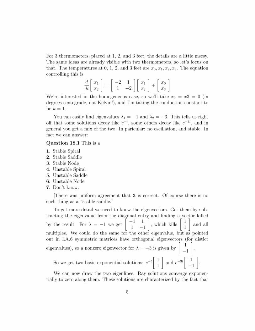
For 3 thermometers, placed at 1, 2, and 3 feet, the details are a little msesy.The same ideas are already visible with two thermometers, so let’s focus onthat. The temperatures at 0, 1, 2, and 3 feet are x0, x1, x2, x3. The equationcontrolling this is
d
dt
[x1x2
]=
[−2 11 −2
][x1x2
]+
[x0x3
]We’re interested in the homogeneous case, so we’ll take x0 = x3 = 0 (indegrees centegrade, not Kelvin!), and I’m taking the conduction constant tobe k = 1.
You can easily find eigenvalues λ1 = −1 and λ2 = −3. This tells us rightoff that some solutions decay like e−t, some others decay like e−3t, and ingeneral you get a mix of the two. In paricular: no oscillation, and stable. Infact we can answer:
Question 18.1 This is a
1. Stable Spiral2. Stable Saddle3. Stable Node4. Unstable Spiral5. Unstable Saddle6. Unstable Node7. Don’t know.
[There was uniform agreement that 3 is correct. Of course there is nosuch thing as a “stable saddle.”
To get more detail we need to know the eigenvectors. Get them by sub-tracting the eigenvalue from the diagonal entry and finding a vector killed
by the result. For λ = −1 we get
[−1 11 −1
], which kills
[11
]and all
multiples. We could do the same for the other eigenvalue, but as pointedout in LA.6 symmetric matrices have orthogonal eigenvectors (for distict
eigenvalues), so a nonzero eigenvector for λ = −3 is given by
[1−1
].
So we get two basic exponential solutions: e−t[
11
]and e−3t
[1−1
].
We can now draw the two eigenlines. Ray solutions converge exponen-tially to zero along them. These solutions are characterized by the fact that
5

the ratio between x1 and x2 is constant in time. These are the normalmodes for the heat model. The Wikipedia definition was applicable onlyto oscillating motion. You know, the word “normal mode” is like the word“happiness.” It’s hard to define, you know it when you see it, and it’s reallyimportant, the basis of everything.
Other solutions are a mix of these two normal modes. IMPORTANT: Thesmaller the (real part of) the eigenvalue, the quicker the decay. e−3t = (e−t)3,so when e−t = 0.1, e−3t = 0.001. So the component of v2 decays muchmore rapidly than the component of v1, so these other trajectories approachtangency with the eigenline for value −1.
[3] Initial conditions.
Suppose I have a different initial condition, maybe
[12
]: so the temper-
atures are 0, 1, 2, 0. What happens? What are c1 and c2 in
x(t) = c1e−t + c2e
−3t
How can we find c1 and c2?
More generally, when we are studying x = Ax, and we’ve found eigenval-ues λ1, . . . and nonzero eigenvectors v1, . . ., the general solution is
x(t) = c1eλ1tv1 + c2e
λ2tv2 + · · ·
We’re interested in the cofficients ci giving specified initial condition x(0) =v. Since eλ·0 = 1 alwasy, our equation is
v = c1v1 + · · ·+ cnvn
As with many computations, the first step is to rewrite this as a matrixequation:
v =[v1 · · · vn
] c1...cn
We will write S for the matrix whose columns are the eigenvectors, so v =
6

S
c1...cn
. Now it’s clear: we find c1, . . . by inverting S:
c1...cn
= S−1v
This is an important principle!
The entries in S−1v are the coefficients in
v = c1v1 + · · ·+ cnvn
In our example, S−1 = 1−2
[−1 −1−1 1
]=
1
2
[1 11 −1
], so
[c1c2
]=
1
2
[1 11 −1
][12
]=
[3/2−1/2
]sou our particular solution is
x(t) =3
2e−t[
11
]− 1
2e−3t
[1−1
]The second term decays much faster than the first.
[4] Coordinates.
The big idea: a system can seem complicated just because we are usingthe wrong coordinates to describe it.
I want to let x be any vector; maybe it varies with time, as a solutionof x = Ax. We can write it as a linear combination of v1, . . ., but now thecoefficients can vary too. I’ll write y1, y2, . . . for them to make them lookmore variable:
x = y1v1 + y2v2 + · · ·
orx = Sy
7

For example, [x1x2
]= x =
[1 11 −1
]y =
[y1 + y2y1 − y2
]This is a change of cooridinates. The y1 axis (where y2 = 0) is the λ1eigenline; the y2 axis (where y1 = 0) is the λ2 eigenline.
We can change back using S−1:
y = S−1x
so for us [y1y2
]=
1
2
[1 11 −1
][x1x2
]i.e.
y1 =x1 + x2
2, y2 =
x1 − x22
[5] Diagonalization.
OK, but these vectors vi have something to do with the matrix A: theyare eigenvectors for it. What does this mean about the relationship betweenS and A? Well, the eigenvector equation is
Av = λv
that is,Av1 = λ1v1 , · · · , Avn = λnvn
Line these up as the columns of a matrix product:
AS = A[v1 · · · vn
]=[λ1v1 · · · λnvn
]Now comes a clever trick: the right hand side is a matrix product as well:
· · · =[v1 · · · vn
]λ1 0 · · · 00 λ2 · · · 0...
.... . .
...0 0 · · · λn
= SΛ
where Λ (that’s a big “lambda”) is the “eigenvalue matrix,” with little λ’sdown the diagonal. That is:
AS = SΛ
8

orA = SΛS−1
This is a diagonalization of A. It exhibits the simlicity hidden inside of A.There are only n eigenvalues, but n2 entries in A. They don’t completelydetermine A, of course, but they say a lot about it.
[6] Decoupling.
Now let’s apply this to the differential equation x = Ax. I’m going toplug
x = Sy and A = SΛS−1
into this equation.
x =d
dtSy = Sy
andAx = SΛS−1x = SΛy
Put it together and cancel the S:
y = Λy
Spelling this out:y1 = λ1y1y2 = λ2y2· · ·
yn = λnyn
Each variable keeps to itself; its derivatives don’t depend on the other vari-ables. They are decoupled.
In our example,
y1 = x1+x22
satisfies y1 = −y1y2 = x1−x2
2satisfies y3 = −3y2
So the smart variables to use to record the state of our insulated barare not x1 and x2, but rather the average and the difference (or half thedifference). The average decays exponentially like e−t. The difference decaysmuch faster. So quite quickly, the two temperatures become very close, andthen the both of them die off exponentially to zero.
9

18.03 LA.10: The Matrix Exponential
[1] Exponentials[2] Exponential matrix[3] Fundamental matrices[4] Diagonalization[5] Exponential law
[1] Exponentials
What is ex?
Very bad definition: ex is the xth power of the number e ∼ 2.718281828459045 . . .
Two problems with this: (1) What is e? (2) What does it mean to raisea number to the power of, say,
√2, or π?
Much better definition: y(x) = ex is the solution to the differential equa-
tiondy
dx= y with initial condition y(0) = 1.
Now there’s no need to know about e in advance; e is defined to be e1.And ex is just a function, which can be evaluated at
√2 or at π just as easily
as at an integer.
Note the sublety: you can’t use this definition to describe ex for any singlex (except x = 0); you need to define the entire function at once, and thenevaluate that function at the value of x you may want.
As you know, this gives us solutions to other equations: I claim that
y = ert satisfiesdy
dt= ry. This comes from the chain rule, with x = rt:
dy
dt=dx
dt
dy
dx= ry
A further advantage of this definition is that it can be extended to othercontexts in a “brain-free” way.
A first example is Euler’s definition
eiθ = cos θ + i sin θ
1

We defined x(t) = e(a+bi)t to be the solution to x = (a + bi)x, and thencalculated that
e(a+bi)t = eat(cos(bt) + i sin(bt))
In all these cases, you get the solution for any initial condition: ertx(0)is the solution to x = rx with initial condition x(0).
[2] Matrix exponential
We’re ready for the next step: We have been studying the equation
dx
dt= Ax
where A is a square (constant) matrix.
Definition. eAt is the matrix of functions such that the solution to x = Ax,in terms of its initial condition, is eAtx(0).
How convenient is that!
If we take x(0) to be the vector with 1 at the top and 0 below, the producteAtx(0) is the first column of eAt. Similarly for the other columns. So:
Each column of eAt is a solution of x = Ax. We could write this:
d
dteAt = AeAt
eAt is a matrix-valued solution! It satisfies a simple initial condition:
eA0 = I
Not everything about 1× 1 matrices extends to the general n×n matrix.But everything about 1×1 matrices does generalize to diagonal n×nmatrices.
If A = Λ =
[λ1 00 λ2
], the given coordinates are already decoupled: the
equation x = Ax is just x1 = λ1x1 and x2 = λ2x2. Plug in initial condition[10
]: the first column of eΛt is
[eλ1t
0
]. Plug in initial condition
[01
]: the
second column is
[0eλ2t
]. So
eΛt =
[eλ1t 00 eλ2t
]2

Same works for n× n, of course.
[3] Fundamental matrices
Here’s how to compute eAt. Suppose we’ve found the right number (n)independent solutions of x = Ax: say u1(t), . . . ,un(t). Line them up in arow: this is a “fundamental matrix” for A:
Φ(t) =[
u1 u2 · · · un
]The general solution is
x(t) = Φ(t)
c1...cn
Φ(t) may not be quite eAt, but it’s close. Note that x(0) = Φ(0)
c1...cn
,
or
c1...cn
= Φ(0)−1x(0). Thus
x(t) = Φ(t)Φ(0)−1x(0)
SoeAt = Φ(t)Φ(0)−1
for any fundamental matrix Φ(t).
Example: A =
[0 −11 0
]. Characteristic polynomial pA(λ) = λ2+1, so the
eigenvalues are ±i. The phase portrait is a “center.” Eigenvectors for λ = i
are killed by A − iI =
[−i 11 −i
]; for example
[1i
]. So the exponential
solutions are given by
eit[
1i
]= (cos t+ i sin t)
[1i
]and its complex conjugate. To find real solutions, take just the right linearcombinations of these to get the real and imaginary parts:
u1(t) =
[cos t− sin t
], u2(t) =
[sin tcos t
]3

These both parametrize the unit circle, just starting at different places. Thecorresponding fundamental matrix is
Φ(t) =
[cos t sin t− sin t cos t
]We luck out, here: Φ(0) = I, so
eAt =
[cos t sin t− sin t cos t
]
[4] Diagonalization
Suppose that A is diagonalizable: A = SΛS−1.
Example: A =
[1 20 3
]. You can find the eigenvalues as roots of the
characteristic polynomial, but you might as well remember that the eigenval-ues of an upper (or lower) triangular matrix are the diagonal entries: here 1
and 3. Also an eigenvalue for 1 is easy: v1 =
[10
]. For the other, subtract
3 from the diagonal entries:
[−2 20 0
]kills v2 =
[11
].
So
S =
[1 10 1
], Λ =
[1 00 3
]Suppose A = SΛS−1. Then we have exponential solutions corresponding
to the eigenvalues:u1(t)eλ1tv1 , . . .
These give a fine fundamental matrix:
Φ(t) =[eλ1tv1 . . . eλntvn
]= SeΛt , S =
[u1 . . . un
],Λ =
λ1
. . .
λn
Then Φ(0) = S, so
eAt = SeΛtS−1
4

In our example,
eAt =
[1 10 1
][et 00 e3t
][1 −10 1
]You could multiply this out, but, actually, the exponential matrix is often apain in the neck to compute, and is often more useful as a symbolic device.Just like ex, in fact!
[5] The exponential law
I claim thateA(t+s) = eAteAs
This is a consequence of “time invariance.” We have to see that both sidesare equal after multiplying by an arbitrary vector v. Let x(t) be the solutionof x = Ax with initial condtion x(0) = v: so x(t) = eAtv. Now fix s and let
y(t) = x(t+ s) = eA(t+s)v
Calculate using the chain rule:
d
dty(t) =
d
dtx(t+ s) = x(t+ s) = Ax(t+ s) = Ay(t)
So y is the solution to y = Ay with y(0) = x(s) = eAsv. That means thaty(t) = eAteAsv. QED
This is the proof of the exponential law even in the 1 × 1 case; and youwill recall that as such it contains the trigonometric addition laws. Powerfulstuff!
5

18.03 LA.11: Inhomogeneous Systems
[1] Planetarium[2] Romance[3] Family[4] Variations[5] Exponential Input/Response
[1] Planetarium
So now we have a symbol expressing a solution of
x = Ax
in terms of initial conditions:
x(t) = eAtx(0)
We saw for example that for A =
[0 −11 0
]
eAt =
[cos t − sin tsin t cos t
][I used the opposite signs on Monday; the calculation is the same.] I want youto have the following vision: The differential equation causes a flow aroundthe origin. As time increases, the whole plane rotates. The differentialequation says: the velocity vector is always perpendicular to the positionvector (and points off to the left). After a time t has elapsed, whateverstarting vector you had has rotated by t radians, counterclockwise.
So let’s see: If I start at v and let s seconds elapse, I’m at eAsv. Then Ilet another t seconds elapse. The effect is that I rotate this new vector by tradians:
eAt(eAs)v
On the other hand, all that has happened is that t + s seconds has elapsedsince time 0, so
eAteAsv = eA(t+s)v
1

This is the exponential law. I had you thinking of the rotation matrix, but thesame reasoning works in complete generality. (Note that I used associativity.)
It shows for example that
(eAt)−1 = e−At
I think you need another example.
[2] The Romance of matrices
The MIT Humanities people have analyzed the plot of Shakespeare’sRomeo and Juliet, and determined that it is well modeled by the followingsystem of equations. The two parameters are
R = Romeo’s affection for Juliet
J = Juliet’s affection for Romeo
These two young people are totally unaffected by any outside influences; thiswill be a homogeneous system. Romeo’s affection for Juliet changes overtime. The rate of change is based on how he currently feels and also onhow she currently feels. Similarly for Juliet. The Humanities people havediscovered that
R = R− J , J = R + J
that isd
dt
[RJ
]=
[1 −11 1
] [RJ
]So Juliet is a straightforward girl: if she likes him, that causes her to start
to like him better. If he likes her, same thing.
Romeo is more complicated. If he likes her, that causes him to start tolike her even more. That’s normal. But if he sees that she is starting to likehim, well, that exerts a negative influence on his feelings towards her.
Question 20.1. This relationship
1. is stable and will settle down to calm old age along a spiral2. is stable and will settle down along a node3. is unstable and will blow up along a node4. is unstable and will probably blow up along a saddle
2

5. is unstable and will spiral out of control6. Who’s Shakespeare?
Let’s see how this plot develops. As the play opens, Romeo has noticedJuliet at a dance, and immediately R = 1. Juliet is otherwise occupied,
though, and J = 0. But the deriviative is
[11
]: a promising sign.
Soon she does notice him and her affection rises. That very fact slows hisgrowth of passion, though, so the plot trajectory curves down. Notice thatR = 0 when R = J : he peaks out when their affections towards each otherare equal.
This continues. The more she likes him, the stronger a drag that is onhis growth of affection for her, till he starts to actively dislike the girl. Thiscontinues till Juliet starts to lose heart. J = 0 when J = −R. Then shestarts to like him less; but she still does love him, so that causes Romeo tolike her less, with predictable effects on her feelings towards him.
Presently her feelings become negative, and his continue to crater, but asshe like him less he gets more interested. His feelings bottom out over here,but she continues to stay away. She starts to flirt with his friends. Things arevery bad, but his complicated nature brings things around. Soon he startsto like her again; that decreases her rate of decline, and soon she bottomsout. As he gets more passionate, she does too, and after a while we’re backto J = 0.
But what’s R now? Well, you can work it out. For the present, let’s justnotice that trA = 2 and detA = 2. This puts us in the unstable part of thespiral segment, so we could have predicted all this quite simply.
Shall we solve? pA(λ) = λ2−2λ+2 = (λ−1)2+1 has roots 1±i. Positivereal part, nonzero imaginary part: so unstable spiral. Eigenvectors for 1 + i
are killed by A − (1 + i)I =
[−i 1−1 −i
]; for example
[1i
]. So exponential
solution e(1+i)t[1i
], with real part u1(t) = et
[cos t− sin t
]and imaginary part
u2(t) = et[
sin tcos t
]. The general solution is a linear combination. Luckily the
starting point we had above is here: our story line was u1.
We’re in luck here again: these two solutions are normalized and we’ve
3

computed that
eAt = et[
cos t sin t− sin t cos t
]The second factor is the rotation matrix we had above. So as time increases,the whole romance spins around while expanding exponentially. After onerotation, 2π time has elapsed, so now R = e2π ∼ 535.49! So my picturewasn’t very accurate.
[3] Inhomogeneous
Of course this is somewhat oversimplified. The fact is that Romeo andJuliet were influenced by their families, the Montagues and Capulets. So thisis not a homogeneous situation after all. A better model might be:
d
dt
[RJ
]=
[1 −11 1
] [RJ
]−[1010
]The two families in Verona agree on one thing: this romance is a terribleidea. Will they succeed in damping it down?
What’s the general form of the answer going to be?
We’ve learned to look for
x = xp + xh
We know about xh. What might we take for a particular solution, with thisconstant forcing term (parental pressure)?
How about trying for a constant solution? It would have to be so thatthe left hand side is zero, so[
1 1−1 1
] [RJ
]=
[1010
]This we can do; we have to compute[
1 −11 1
]−1
=1
2
[1 1−1 1
]so
xp =1
2
[1 1−1 1
] [1010
]=
[100
]4

So there is a stable point, an equilibrium, where R = 10 and J = 0, wheneverything is in balance. It must be quite uncomfortable for poor Romeo.But as soon as someone exhales, you add in a nonzero homogeneous equationand the couple quickly spirals out of control. This is an unstable equilibrium!The attempt at parental control works only if Romeo and Juliet happen tobe in this state; and it’s very unlikely to work for very long.
[4] Variations But what if the input signal here isn’t constant? I want tosolve
x = Ax + q(t) or x− Ax = q
Again it suffices to find a single “particular solution.”
Let’s try what we did before: “variation of parameters.” We know thatthe general solution to x = Ax is of the form
c1u1(t) + · · ·+ cnun(t)
where u1, . . . ,un are independent solutions, and we now have a slick way towrite this, using the corresponding “fundamental matrix”
Φ(t) =[u1(t) u2(t) · · · un(t)
]The fact that the columns are solutions is recorded by the matrix equation
d
dtΦ(t) = AΦ(t)
We can write the general solution of the homogeneous equation as Φ(t)c.The coefficient vector c is a vector of “parameters.” Let’s let it vary: try for
x(t) = Φ(t)u(t)
Plug into the equation:
x(t) = AΦ(t)u(t) + Φ(t)u(t)−Ax(t) = −AΦ(t)u(t)
q(t) = Φ(t)u(t)
Solve for u:u(t) = Φ(t)−tq(t)
5

Then integrate and multiply by Φ(t)−1:
x(t) = Φ(t)
∫Φ(t)−1q(t) dt
Notice that the indefinite integral is only well defined up to adding aconstant vector, which then gets multiplied by Φ(t): so this is the generalsolution in a nutshell.
Since we don’t care about initial conditions at this point, there’s no needto use the exponential matrix and it’s generally more convenient not to. Ifyou do, though, you can use the fact that (eAt)−1 = e−At to write
x = eAt∫e−Atq(t) dt
[5] Exponential Input/Response
In this section we consider exponential input signals. Recall two thingsabout ordinary constant coefficient equations. First, with exponential inputwe can use the method of optimism which leads to algebraic methods. Sec-ond, using complex replacement sinusoidal input signals can be handled inthe same way as exponential signals.
Let A be a constant matrix, a a constant and K a constant column vector.We consider here the system
x = Ax + eatK
To solve this equation we use the method of optimism and try a particularsolution of the form xp = eatv, where v is an unknown constant vector.Substituting xp into the equation and doing some simple algebra we find
xp = Ax + eatK⇔ aeatv = eatAv + eatK⇔ (aI − A)v = K⇔ v = (aI − A)−1K⇔ xp = eatv
= eat(aI − A)1K
Notes: 1. In the third equation we replaced av by aIv. The identity matrixchanges nothing, but allows us to do the algebra of matrix subtraction.
6
2. This is only valid if (aI − A)−1 exists, that is if det(aI − A) 6= 0. (Note,this is equivalent to saying a is not an eigenvalue of A.)
Following our usage for ordinary differential equations we call the formulax = eat(aI−A)−K the exponential response formula or the exponential inputtheorem.
Examples
1. Solvex = 3x− y + e2t
y = 4x− y − e2t
Solution. Here A =
[3 −14 −1
], a = 2, K =
[1−1
].
(2I − A)−1 =
[−1 1−4 3
]−1
=
[3 −14 −1
]⇒ xp = e2t
[3 −14 −1
] [1−1
]= e2t
[45
].
2. (Same matrix as in example 1.) Solve
x = 3x− y + 3
y = 4x− y + 2
Solution: a = 0, K =
[32
], −A−1 = −
[−1 1−4 3
]=
[1 −14 −3
].
xp = −A−1 ·K =
[1 −14 −3
] [32
]=
[16
].
Note: Here the input is a constant so our method of optimism is equivalentto guessing a constant solution.
3. Solvex = x+ 2y + cos t
y = 2x+ y
Solution: We use complex replacement:
z =
[1 22 1
]z + eit
[10
]x = Re (z).
The exponential response formula gives
zp(t) = eit(iI − A)−1
[10
]7

We have
iI − A =
[i− 1 −2−2 i− 1
]⇒ (iI − A)−1 =
1
−4− 2i
[i− 1 2
2 i− 1
]So (not showing all of the complex arithmetic),
zp(t) = 1−4−2i
eit[i− 1 2
2 i− 1
] [10
]= (cos t+ i sin t) 1
10
[1− 3i−4 + 2i
]= 1
10
([cos t+ 3 sin t−4 cos t− 2 sin t
]+ i
[−3 cos t+ sin t2 cos t− 4 sin t
])
xp(t) = Re (zp)(t) = 110
[cos t+ 3 sin t−4 cos t− 2 sin t
]=
[xpyp
]
SuperpositionFor linear constant coefficient equations the principle of superposition allows
us to use the exponential input method for input functions like f =
[3e2t
−et].
That is we can split f into a sum:
f =
[3e2t
−et]
= e2t[30
]+ et
[0−1
].
and solve with each piece separately and then sum the two solutions.
8

18.03 PDE.1: Fourier’s Theory of Heat
1. Temperature Profile.
2. The Heat Equation.
3. Separation of Variables (the birth of Fourier series)
4. Superposition.
In this note we meet our first partial differential equation (PDE)
∂u
∂t= k
∂2u
∂x2
This is the equation satisfied by the temperature u(x, t) at position x and time t of a bardepicted as a segment,
0 ≤ x ≤ L, t ≥ 0
The constant k is the conductivity of the material the bar is made out of.
We will focus on one physical experiment. Suppose that the initial temperature is 1, andthen the ends of the bar are put in ice. We write this as
u(x, 0) = 1, 0 ≤ x ≤ L u(0, t) = 0, u(L, t) = 0, t > 0 .
The value(s) of u = 1 at t = 0 are called initial conditions. The values at the ends are calledendpoint or boundary conditions. We think of the initial and endpoint values of u as theinput, and the temperature u(x, t) for t > 0, 0 < x < L as the response. (For simplicity,we assume that only the ends are exposed to the lower temperature. The rest of the baris insulated, not subject to any external change in temperature. Fourier’s techniques alsoyield answers even when there is heat input over time at other points along the bar.)
As time passes, the temperature decreases as cooling from the ends spreads toward themiddle. At the midpoint, L/2, one finds Newton’s law of cooling,
u(L/2, t) ≈ ce−t/τ , t > τ
The so-called characteristic time τ is inversely proportional to the conductivity of the ma-terial. If we choose units so that τ = 1 for copper, then according to Wikipedia,
τ ∼ 7 (cast iron); τ ∼ 7000 (dry snow)
The constant c, on the other hand, is universal:
c ≈ 1.3
It depends only on the fact that the shape is a bar (modeled as a line segment).
Fourier figured out not only how to explain c using differential equations, but the whole
temperature profile: u(x, t) ≈ e−t/τh(x); h(x) =4
πsin(πLx), t > τ.
The shape of h reflects how much faster the temperature drops near the ends than in themiddle. It’s natural that h should be some kind of hump, symmetric around L/2.
We looked at the heat equation applet to see this profile emerge as t increases. It’sremarkable that a sine function emerges out of the input u(x, 0) = 1. There is no evident
1

mechanism creating a sine function, no spring, no circle, no periodic input. The sine functionand the number 4/π arise naturally out of differential equations alone.
Deriving the heat equation. To explain the heat equation, we start with a thoughtexperiment. If we fix the temperature at the ends, u(0, t) = 0 and u(L, t) = T , what willhappen in the long term as t→∞? The answer is that
u(x, t)→ Usteady(x), t→∞
where Usteady is the steady, or equilbrium, temperature, and
Usteady(x) =T
Lx (linear)
The temperature u(L/2, t) at the midpoint L/2 tends to the average of 0 and T , namelyT/2. At the point L/4, half way between 0 and L/2, the temperature tends to the averageof the temperature at 0 and T/2, and so forth.
At a very small scale, this same mechanism, the tendency of the temperature profiletoward a straight line equilibrium means that if u is concave down then the temperature inthe middle should decrease (so the profile becomes closer to being straight). If u is concaveup, then the temperature in the middle should increase (so that, once again, the profilebecomes closer to being straight). We write this as
∂2u
∂x2< 0 =⇒ ∂u
∂t< 0
∂2u
∂x2> 0 =⇒ ∂u
∂t> 0
The simplest relationship that reflects this is a linear (proportional) relationship,
∂u
∂t= k
∂2u
∂x2, k > 0
Fourier’s reasoning. Fourier introduced the heat equation, solved it, and confirmed inmany cases that it predicts correctly the behavior of temperature in experiments like theone with the metal bar.
Actually, Fourier crushed the problem, figuring out the whole formula for u(x, t) and notjust when the initial value is u(x, 0) = 1, but also when the initial temperature varies withx. His formula even predicts accurately what happens when 0 < t < τ .
Separation of Variables. For simplicity, take L = π and k = 1. The idea is not to tryto solve for what looks like the simplest initial condition namely u(x, 0) = 1, but instead tolook for solutions of the form
u(x, t) = v(x)w(t)
Plugging into the equation, we find
∂u
∂t= v(x)w(t),
∂2u
∂2x= v′′(x)w(t)
Therefore, since k = 1,
v(x)w(t) = v′′(x)w(t) =⇒ w(t)
w(t)=v′′(x)
v(x)= c (constant).
2

This is the first key step. We divided by v(x) and w(t) to “separate” the variables. Butthe function w(t)/w(t) is independent of x, whereas v′′(x)/v(x) is indendent of t. And sincethese are equal, this function depends neither on x nor on t, and must be a constant. Noticealso that the constant, which we are calling c for the time being, is the same constant intwo separate ordinary differential equations:
w(t) = cw(t), v′′(x) = cv(x).
The best way to proceed is to remember the endpoint conditions
u(0, t) = u(π, 0) = 0 =⇒ v(0) = v(π) = 0.
We know what the solutions to v′′(x) = cv(x), v(0) = v(π) = 0 look like. They are
vn(x) = sinnx, n = 1, 2, 3, . . .
Moreover, v′′n(x) = −n2 sinnx = −n2vn(x), so that c = −n2. We now turn to the equationfor w, which becomes
wn(t) = −n2w(t) =⇒ wn(t) = e−n2t.
(We may as well take w(0) = 1. We will be taking multiples later.) In summary, we havefound a large collection of solutions to the equation, namely,
un(x, t) = vn(x)wn(t) = e−n2t sinnx
For these solutions, the endpoint condition un(0, t) = un(π, t) = 0 is satisfied, but the initialcondition is
un(x, 0) = vn(x) = sinnx .
This is where Fourier made an inspired step. What if we try to write the function u(x, 0) = 1as a linear combination of vn(x) = sinnx?
On the face of it, expressing 1 as a sum of terms like sinnx makes no sense. We knowthat sinnx is zero at the ends x = 0 and x = π. But something tricky should be happeningat the ends because the boundary conditions are discontinuous in time. At t = 0 wehad temperature 1 at the ends, then suddenly when we plunged the ends in ice, we hadtemperature 0. So it’s not crazy that the endpoints should behave in a peculiar way.
If there is any chance to write
u(x, 0) = 1 =∑
bn sinnx, 0 < x < π,
then it must be that the function is odd. In other words, we need to look at
f(x) =
{1 0 < x < π
−1 −π < x < 0
Moreover, the function has to be periodic of period 2π. This is none other than the squarewave f(x) = Sq(x), the very first Fourier series we computed.
1 = Sq(x) =4
π
(sinx+
1
3sin 3x+
1
5sin 5x+
), 0 < x < π.
Now since initial conditions vn(x) yield the solution un(x, t), we can apply the
Principle of Superposition u(x, 0) =∑
bn sinnx =⇒ u(x, t) =∑
bne−n2t sinnx
3

In other words, if u(x, 0) = 1, 0 < x < π, then
u(x, t) =4
π
(e−t sinx+
1
3e−3
2t sin 3x+1
5e−5
2t sin 5x+ · · ·)
0 ≤ x ≤ π, t > 0.
The exact formula for the solution u to the heat equation is this series; it cannot beexpressed in any simpler form. But often one or two terms already give a good approx-imation. Fourier series work as well, both numerically and conceptually, as any finite sumof terms involving functions like e−t and sinx. Look at the Heat Equation applet to see thefirst term (main hump) emerge, while the next term b3e
−9t sin 3x tends to zero much morequickly. (The other terms are negligible after an even shorter time.)
For this example, the characteristic time is τ = 1, e−t/τ = e−t, and
u(x, t) =4
πe−t sinx+ smaller terms as t→∞.
To get an idea how small the smaller terms are, take an example.
Example. Fix t1 = ln 2, then e−t1 = 1/2, and
u(x, t1) =4
π
(1
2sinx+
1
3 · 29sin 3x+ · · ·
)=
2
πsinx± 10−3
4

18.03 PDE.2: Decoupling; Insulated ends
1. Normal Modes: eλktvk
2. Superposition
3. Decoupling; dot product
4. Insulated ends
In this note we will review the method of separation of variables and relate it to linearalgebra. There is a direct relationship between Fourier’s method and the one we used tosolve systems of equations.
We compare a system of ODE u(t) = Au(t) where A is a matrix and u(t) is a vector-valued function of t to the heat equation
∂u
∂t=
∂2
∂x2u, 0 < x < π, t > 0; u(0, t) = u(π, t) = 0
with zero temperature ends. To establish the parallel, we write
u(t) = Au(t) −−−−− u =∂u
∂t=
∂2
∂x2u (A = (∂/∂x)2)
To solve the equations we look for normal modes:
Try u(t) = w(t)v. −−−−− Try u(x, t) = w(t)v(x).
This leads to equations for eigenvalues and eigenvectors:{Av = λv
w = λw−−−−−−
{Av = v′′(x) = λv(x) [and v(0) = v(π) = 0]
w(t) = λw(t)
There is one new feature: in addition to the differential equation for v(x), there are endpointconditions. The response to the system u = Au is determined by the initial condition u(0),but the heat equation response is only uniquely identified if we know the endpoint conditionsas well as u(x, 0).
Eigenfunction Equation. The solutions to
v′′(x) = λv(x) and v(0) = v(π) = 0,
are known as eigenfunctions. They are
vk(x) = sin kx, k = 1, 2, . . .
and the eigenvalues λk = −k2 lead to wk(t) = e−k2t.
normal modes : eλktvk −−−−−− e−k2t sin(kx)
The principle of superposition, then says that
u(0) =∑
ckvk =⇒ u(t) =∑
ckeλktvk
and, similarly,
u(x, 0) =∑
bk sin kx =⇒ u(x, t) =∑
bke−k2t sin kx
1

More generally, we will get formats for solutions of the form
u(x, t) =∑
bke−βk2t sin(αkx) or cosines
The scaling will change if the units are different (inches versus meters in x; seconds versushours in t) and depending on physical constants like the conductivity factor in front of the(∂/∂x)2 term, or if the interval is 0 < x < L instead of 0 < x < π. Also, we’ll see anexample with cosines below.
The final issue is how to find the coefficients ck or bk. If we have a practical way to findthe coefficients ck in
u(0) =∑
ckvk,
then we say we have decoupled the system. The modes eλktvk evolve according to separateequations wk = λkwk.
Recall that the dot product of vectors is given, for example, by123
· 2−10
= 1 · 2 + (2)(−1) + 3 · 0 = 0
When the dot product is zero the vectors are perpendicular. We can also express the lengthsquared of a vector in terms of the dot product:
v =
123
; v · v =
123
·1
23
= 12 + 22 + 32 = (length)2 = ‖v‖2
There is one favorable situation in which it’s easy to calculate the coefficients ck, namelyif the eigenvectors vk are perpendicular to each other
vk ⊥ v` ⇐⇒ vk · v` = 0
This happens, in particular, if the matrix A is symmetric. In this case we also normalizethe vectors so that their length is one:
‖vk‖2 = vk · vk = 1
Thenck = vk · u(0)
The proof is
vk(c1v1 + · · ·+ cnvn) = 0 + · · ·+ 0 + ckvk · vk + 0 + · · · = ck .
The same mechanism is what makes it possible to compute Fourier coefficients. We have
vk ⊥ v` ⇐⇒∫ π
0
vk(x)v`(x) dx = 0
and ∫ π
0
vk(x)2 dx =
∫ π
0
sin2(kx) dx =π
2
2

To compensate for the length not being 1 we divide by the factor π/2. It follows that
bk =2
π
∫ π
0
u(x, 0) sin(kx) dx
The analogy between these integrals and the corresponding dot products is very direct.When evaluating integrals, it makes sense to think of functions as a vectors
~f = [f(x1), f(x2), . . . , f(xN )]; ~g = [g(x1), g(x2), . . . , g(xN )].
The Riemann sum approximation to an integral is written∫ π
0
f(x)g(x) dx ≈∑j
f(xj)g(xj)∆x = ~f · ~g∆x
We have not explained the factor ∆x, but this is a normalizing factor that works out aftertaking into account proper units and dimensional analysis. To repeat, functions are vectors:we can take linear combinations of them and even use dot products to find their “lengths”and the angle between two of them, as well as distances between them.
Example 1. Zero temperature ends. We return to the problem from PDE.1, in whichthe initial conditions and end point conditions were
u(x, 0) = 1 0 < x < π; u(0, t) = u(π, t) = 0 t > 0.
Our goal is to express
1 =
∞∑1
bk sin(kx), 0 < x < π
The physical problem does not dictate any value for the function u(x, 0) outside 0 < x < π.But if we want it to be represented by this sine series, it’s natural to consider the oddfunction
f(x) =
{1 0 < x < π
−1 −π < x < 0
Moreover, because the sine functions are periodic of period 2π, it’s natural to extend f tohave period 2π. In other words, f(x) = Sq(x), the square wave. We computed this seriesin L26 (same formula as above for bk) and found
f(x) =4
π
(sinx+
sin 3x
3+
sin 5x
5+ · · ·
)Therefore the solution is
u(x, t) =4
π
(e−t sinx+ e−3
2t sin 3x
3+ · · ·
)
Example 2. Insulated Ends.
When the ends of the bar are insulated, we have the usual heat equation (taken here forsimplicity with conductivity 1 and on the interval 0 < x < π) given by
∂u
∂t=∂2u
∂x2, 0 < x < π, t > 0,
3

with the new feature that the heat flux across 0 and π is zero. This is expressed by theequations
insulated ends :∂u
∂x(0, t) =
∂u
∂x(π, t) = 0 t > 0
Separation of variables u(x, t) = v(x)w(t) yields a new eigenfunction equation:
v′′(x) = λv(x), v′(0) = v′(π) = 0
whose solution arevk(x) = cos(kx), k = 0, 1, 2 . . .
Note that the index starts at k = 0 because cos 0 = 1 is a nonzero function. The eigenvaluesare λk = −k2, but now the first eigenvalue is
λ0 = 0.
This will make a difference when we get to the physical interpretation. Since wk(t) =−k2wk(t), we have
wk(t) = e−k2t
and the normal modes aree−k
2t cos(kx), k = 0, 1, . . .
The general solution has the form (or format)
u(x, t) =a02e0t +
∞∑1
ake−k2t cos(kx)
(Here we have anticipated the standard Fourier series format by treating the constant termdifferently.)
Let us look at one specific case, namely, initial conditions
u(x, 0) = x, 0 < x < π
We can imagine an experiment in which the temperature of the bar is 0 on one end and 1 onthe other. After a fairly short period, it will have stabilized to the equilibrium distributionx. Then we insulate both ends (cease to provide heat or cooling that would maintain theends at 0 and 1 respectively). What happens next?
To find out we need to express x as a cosine series. So we extend it evenly to
g(x) = |x|, |x| < π, with period 2π
This is a triangular wave and we calculated its series using g′(x) = Sq(x) as
g(x) =a02− 4
π
(cosx+
cos 3x
32+
cos 5x
52+ · · ·
)The constant term is not determined by g′(x) = Sq(x) and must be calculated separately.Recall that
a0 =2
π
∫ π
0
g(x) cos 0 dx =2
π
∫ π
0
x dx =x2
π
∣∣∣∣π0
= π
4

Put another way,a02
=1
π
∫ π
0
g(x) dx = average(g) =π
2
Thus, putting it all together,
u(x, t) =π
2− 4
π
(e−t cosx+ e−3
2t cos 3x
32+ · · ·
)Lastly, to check whether this makes sense physically, consider what happens as t→∞.
In that case,
u(x, t)→ π
2
In other words, when the bar is insulated, the temperature tends to a constant equal to theaverage of the initial temperature.
5

18.03 PDE.3: The Wave Equation
1.∂2u
∂t2= c2
∂2u
∂x22. Normal Modes.3. Wave fronts and wave speed (d’Alembert solution).4. Real life waves.
I showed you an elastic band which oscillated. In the literature this is usually referred toas a vibrating string. Let u(x, t) represent the vertical displacement of the string. In otherwords, for each fixed time t, the graph of the string is y = y(x) = u(x, t).
Consider, as in the case of the heat equation, the equilibrium position in which theelastic string is not moving. In that case, it’s in a straight line. If the string is concavedown (curved above the equilibrium) then the elasticity pulls the string back down in themiddle. This tendency is a restoring force like that of a spring. Since force is proportionalto acceleration (F = ma), and acceleration is ∂2u/∂t2, we have
∂2u
∂x2< 0 =⇒ ∂2u
∂t2< 0.
Similarly for concave up configurations,
∂2u
∂x2> 0 =⇒ ∂2u
∂t2> 0.
The simplest rule that realizes this effect is proportionality,
∂2u
∂t2= c2
∂2u
∂x2.
We wrote the constant first as c > 0 and rewrote it later as c2 > 0 when it turned out thatthe right units of c are meters per second so that it represents a speed.
Let us take c = 1 for simplicity and fix the ends of the string at 0 and π. The normalmodes have the form
u(x, t) = v(x)w(t), v(0) = v(π) = 0.
Substituting into the equation, we find
w(t)v(x) = w(t)v′′(x),
which leads (via the separation of variables method, w(t)/w(t) = v′′(x)/v(x) = λ) to theequations
v′′(x) = λv(x), v(0) = v(π) = 0.
These are the same as for the heat equation with fixed ends, and we already found a completelist of solutions (up to multiples)
vn(x) = sin(nx), n = 1, 2, 3, . . . .
We also have v′′n(x) = −n2vn(x), so that λn = −n2. What is different this time is that theequation for wn is second order
wn(t) = −n2wn(t)
A second order equation has a two dimensional family of solutions. In this case, they are
wn(t) = a cos(nt) + b sin(nt)
1

This highlights the main conceptual differences between the heat and wave equations. Thesewave equation solutions are oscillatory in t not exponential. Also the extra degree of freedommeans we have to specify not only the initial position u(x, 0), but also the initial velocity(∂/∂t)u(x, 0).
We will take the simplest initial velocity, namely, initial velocity 0 (also the most realisticchoice when we pluck a string). Thus we impose the conditions
0 = wn(0) = −an sin(0) + bn cos 0 = bn =⇒ b = 0
and (for simplicity) wn(0) = a = 1. Now a = 1 and b = 0, so that the normal modes are
un(x, t) = cos(nt) sin(nx)
The principle of superposition says that if
f(x) =
∞∑n=1
bn sin(nx), 0 < x < π
then
u(x, t) =
∞∑n=1
bn cos(nt) sin(nx), 0 < x < π
solves the wave equation with constant c = 1, initial condition u(x, 0) = f(x) and initialvelocity (∂/∂t)u(x, 0) = 0 and endpoint conditions u(0, t) = u(π, t) = 0, t > 0. (Actually,the wave equation is reversible, and these equations are satisfied for −∞ < t <∞.)
Notice that there are now two inputs at time t = 0, the initial position f(x) and theinitial velocity which we have set equal to 0 for simplicity.1 This is consistent with the factthat the equation is second order in the t variable.
Wave fronts. D’Alembert figured out another formula for solutions to the one (space)dimensional wave equation. This works for initial conditions v(x) is defined for all x, −∞ <x <∞. The solution (for c = 1) is
u1(x, t) = v(x− t)
We can check that this is a solution by plugging it into the equation,
∂2
∂t2u(x, t) = (−1)2v′′(x− t) = v′′(x− t) =
∂2
∂x2u(x, t).
Similarly, u2(x, t) = v(x+ t) is a solution.
We plot the behavior of this solution using a space-time diagram and taking the simplestinitial condition, namely the step function,
v(x) =
{1 x < 0
0 x > 0
The solutionu1(x, t) = v(x− t)
1If the initial velocity is not zero, one can write a series solution involving, in addition, the other solutionto the equation for wn(t), namely sin(nt)
2

takes on only two values, 0 and 1. Therefore, we can draw a picture showing how thesolution behaves by drawing the (x, t) plane and dividing the plane into the region whereu1(x, t) = 1 versus u1(x, t) = 0. This kind of space-time diagram is often used to describethe behavior of waves.2 We have
u1(x, t) = v(x− t) = 1 ⇐⇒ x− t < 0 ⇐⇒ t > x,
andu1(x, t) = v(x− t) = 0 ⇐⇒ x− t > 0 ⇐⇒ t < x.
The divider between the places where u1 = 1 and u1 = 0 is known as the wave front and itis located at the line of slope 1,
t = x
We drew this, indicating u1 = 1 above the line t = x and u1 = 0 below.
The only feature we want to extract from this picture is that as time increases, the wavemoves at a constant speed 1. An observer at x = 10 will see the wave front pass (the valueof u(x, t) switch from 0 to 1) at time t = 10. If we were to change the constant c we wouldobtain a solution v(x− ct) whose wave front travels at the speed c.
In order to understand what we are looking at in simulations and real life, we need toenforce both initial conditions, position and velocity. If
u(x, t) = av(x− t) + bv(x+ t)
and u(x, 0) = v(x), (∂/∂t)u(x, 0) = 0, then we have
u(x, 0) = av(x) + bv(x) = v(x) =⇒ a+ b = 1;
(∂/∂t)u(x, 0) = −av′(x) + bv′(x) = 0 =⇒ −a+ b = 0.
Hence,
a = b =1
2; u(x, t) =
1
2(v(x− t) + v(x+ t))
is the solution of interest to us. Plotting the three regions u = 1, u = 1/2 and u = 0, wesee the plane divided by a V shape with 1 on the left 1/2 in the middle and 0 on the right.This says that there is a wave front travelling both left and right from the source. This islike what happens with point sources in higher dimensions. In two dimensions, a pebbledropped in a quiet pond will send a disturbance (wave front) outward in all directions withequal speed, forming a circular wave front. The space-time picture of this wave front lookslike an ice-cream cone. In three dimensions, a source of sound our light will send out wavein all directions. The wave front is an expanding sphere. In one dimension, the geometryis less evident. What is happening is that there are only two possible directions (left andright) instead of a whole circle or sphere of directions.
The next step is to note that it is not realistic for a string to have a jump discontinuitylike the step function. But any feature of the graph will travel at the wave speed. Forexample, if we strech a string to a triangular shape with a kink, then the kink will travel(in both directions) at the wave speed. We looked at this in the applet, and also saw thatwhen the kink hits the fixed ends it bounces off and returns. (The kinks always go at thespeed c; take a look in the applet, in which you can adjust the wave speed.)
Real life waves. Finally, we looked at a slow motion film of an vibrating elastic band at
2In the general theory of relativity, certain rescaled space-time diagrams are used to keep track of lightas it travels into black holes. In that case, they are called Penrose diagrams.
3
http://www.acoustics.salford.ac.uk/feschools/waves/quicktime/elastic2512K_
Stream.mov
The video shows the kink(s) in the band propagating at a steady speed and bouncing offthe ends. This resembles what we saw in the applet. Then we witnessed a new phenomenon:damping. As the system loses energy, all the modes are damped.
The damped wave equation is
∂2u
∂t2+ b
∂u
∂t= c2
∂2u
∂x2, b > 0
This introduces the factor e−bt/2 in the solutions.
Closer examination indicates (not entirely clear without some more detailed numericalsimulation!) that the main mode(s) are revealed more quickly than would be the caseusing a linear damped wave equation. The higher frequency modes are being damped morequickly than the lower frequency ones. A scientist or engineer might say that this systemis exhibiting some nonlinearity in its response. The modes of a linear wave equation wouldall have the same damping constant b. This suggests that one can’t explain fully thisrubber band using linear differential equations alone. It satisfies some nonlinear differentialequation that shares many features with the linear equation, including the wave speed andthe normal modes.
4

18.03 EXERCISES
1. First-order ODE’s
1A. Introduction; Separation of Variables
1A-1. Verify that each of the following ODE’s has the indicated solutions (ci, a are con-stants):
a) y′′ − 2y′ + y = 0, y = c1ex + c2xe
x
b) xy′ + y = x sinx, y =sinx+ a
x− cosx
1A-2. On how many arbitrary constants (also called parameters) does each of the followingfamilies of functions depend? (There can be less than meets the eye. . . ; a, b, c, d, k areconstants.)
a) c1ekx b) c1e
x+a c) c1 + c2 cos 2x+ c3 cos2 x d) ln(ax+ b) + ln(cx+ d)
1A-3. Write down an explicit solution (involving a definite integral) to the followinginitial-value problems (IVP’s):
a) y′ =1
y2 lnx, y(2) = 0 b) y′ =
yex
x, y(1) = 1
1A-4. Solve the IVP’s (initial-value problems):
a) y′ =xy + x
y, y(2) = 0 b)
du
dt= sin t cos2 u, u(0) = 0
1A-5. Find the general solution by separation of variables:
a) (y2 − 2y) dx+ x2dy = 0 b) xdv
dx=
√
1− v2
c) y′ =
(
y − 1
x+ 1
)2
d)dx
dt=
√1 + x
t2 + 4
1B. Standard First-order Methods
1B-1. Test the following ODE’s for exactness, and find the general solution for those whichare exact.
a) 3x2y dx+ (x3 + y3) dy = 0 b) (x2 − y2) dx+ (y2 − x2) dy = 0
c) veuvdu+ yeuvdv = 0 d) 2xy dx− x2dy = 0
1B-2. Find an integrating factor and solve:
a) 2x dx+x2
ydy = 0 b) y dx− (x+ y) dy = 0, y(1) = 1
c) (t2 + 4) dt+ t dx = x dt d) u(du− dv) + v(du+ dv) = 0. v(0) = 11

2 18.03 EXERCISES
1B-3. Solve the homogeneous equations
a) y′ =2y − x
y + 4xb)
dw
du=
2uw
u2 − w2c) xy dy − y2dx = x
√
x2 − y2 dx
1B-4. Show that a change of variable of the form u =y
xnturns y′ =
4 + xy2
x2yinto an
equation whose variables are separable, and solve it.
(Hint: as for homogeneous equations, since you want to get rid of y and y′, begin byexpressing them in terms of u and x.)
1B-5. Solve each of the following, finding the general solution, or the solution satisfyingthe given initial condition.
a) xy′ + 2y = x b)dx
dt− x tan t =
t
cos t, x(0) = 0
c) (x2 − 1)y′ = 1− 2xy d) 3v dt = t(dt− dv), v(1) = 1
4
1B-6. Consider the ODEdx
dt+ax = r(t), where a is a positive constant, and lim
t→∞
r(t) = 0.
Show that if x(t) is any solution, then limt→∞
x(t) = 0. (Hint: use L’Hospital’s rule.)
1B-7. Solve y′ =y
y3 + x. Hint: consider
dx
dy.
1B-8. The Bernoulli equation. This is an ODE of the form y′+p(x)y = q(x)yn, n 6= 1.
Show it becomes linear if one makes the change of dependent variable u = y1−n.
(Hint: begin by dividing both sides of the ODE by yn .)
1B-9. Solve these Bernoulli equations using the method decribed in 1B-8:
a) y′ + y = 2xy2 b) x2y′ − y3 = xy
1B-10. The Riccati equation. After the linear equation y′ = A(x) + B(x) y, in a sensethe next simplest equation is the Riccati equation
y′ = A(x) +B(x)y + C(x)y2,
where the right-hand side is now a quadratic function of y instead of a linear function. Ingeneral the Riccati equation is not solvable by elementary means. However,
a) show that if y1(x) is a solution, then the general solution is
y = y1 + u,
where u is the general solution of a certain Bernoulli equation (cf. 1B-8).
b) Solve the Riccati equation y′ = 1− x2 + y2 by the above method.
1B-11. Solve the following second-order autonomous equations (“autonomous” is an im-portant word; it means that the independent variable does not appear explicitly in theequation — it does lurk in the derivatives, of course.)
a) y′′ = a2y b) yy′′ = y′2
c) y′′ = y′(1 + 3y2), y(0) = 1, y′(0) = 2

SECTION 1: FIRST-ORDER ODE’S 3
1B-12. For each of the following, tell what type of ODE it is — i.e., what method you
would use to solve it. (Don’t actually carry out the solution.) For some, there are several
methods which could be used.
1. (x3 + y) dx+ x dy = 0 2.dy
dt+ 2ty − e−t = 0
3. y′ =x2 − y2
5xy4. (1 + 2p) dq + (2− q) dp = 0
5. cosx dy = (y sinx+ ex) dx 6. x(tan y)y′ = −1
7. y′ =y
x+
1
y8.
dv
du= e2u+3v
9. xy′ = y + xey/x 10. xy′ − y = x2 sinx
11. y′ = (x+ ey)−1 12. y′ +2y
x− y2
x= 0
13.dx
dy= −x
(
2x2y + cos y
3x2y2 + sin y
)
14. y′ + 3y = e−3t
15. xdy
dx− y =
√
x2 + y2 16.y′ − 1
x2= 1
17. xy′ − 2y + y2 = x4 18. y′′ =y(y + 1)
y′
19. tds
dt= s(1− ln t+ ln s) 20.
dy
dx=
3− 2y
2x+ y + 1
21. x2y′ + xy + y2 = 0 22. y′ tan(x+ y) = 1− tan(x+ y)
23. y ds− 3s dy = y4 dy 24. du = −1 + u cos2 t
t cos2 tdt
25. y′ + y2 + (2x+ 1)y + 1 + x+ x2 = 0 26. y′′ + x2y′ + 3x3 = sinx
1C. Graphical and Numerical Methods
1C-1. For each of the following ODE’s, draw a direction field by using about five isoclines;the picture should be square, using the intervals between−2 and 2 on both axes. Then sketchin some integral curves, using the information provided by the direction field. Finally, dowhatever else is asked.
a) y′ = −y
x; solve the equation exactly and compare your integral curves with the
correct ones.
b) y′ = 2x+ y ; find a solution whose graph is also an isocline, and verify this factanalytically (i.e., by calculation, not from a picture).
c) y′ = x− y ; same as in (b).
d) y′ = x2 + y2 − 1
e) y′ =1
x+ y; use the interval −3 to 3 on both axes; draw in the integral curves
that pass respectively through (0, 0), (−1, 1), (0,−2). Will these curves cross the liney = −x− 1? Explain by using the Intersection Principle (Notes G, (3)).

4 18.03 EXERCISES
1C-2. Sketch a direction field, concentrating on the first quadrant, for the ODE
y′ =−y
x2 + y2.
Explain, using it and the ODE itself how one can tell that the solution y(x) satisfying theinitial condition y(0) = 1
a) is a decreasing function for y > 0;b) is always positive for x > 0 .
1C-3. Let y(x) be the solution to the IVP y′ = x− y, y(0) = 1.
a) Use the Euler method and the step size h = .1 to to find an approximate value ofy(x) for x = .1, .2, .3 . (Make a table as in notes G).
Is your answer for y(.3) too high or too low, and why?
b) Use the Modified Euler method (also called Improved Euler, or Heun’s method) andthe step size h = .1 to determine the approximate value of y(.1) . Is the value for y(.1) youfound in part (a) corrected in the right direction — e.g., if the previous value was too high,is the new one lower?
1C-4. Use the Euler method and the step size .1 on the IVP y′ = x+ y2, y(0) = 1, tocalculate an approximate value for the solution y(x) when x = .1, .2, .3 . (Make a table asin Notes G.) Is your answer for y(.3) too high or too low?
1C-5. Prove that the Euler method converges to the exact value for y(1) as the progressivelysmaller step sizes h = 1/n, n = 1, 2, 3, . . . are used, for the IVP
y′ = x− y, y(0) = 1 .
(First show by mathematical induction that the approximation to y(1) gotten by using thestep size 1/n is
yn = 2(1− h)n − 1 + nh .
The exact solution is easily found to be y = 2e−x + x− 1 .)
1C-6. Consider the IVP y′ = f(x), y(0) = y0.
We want to calculate y(2nh), where h is the step size, using n steps of the Runge-Kuttamethod.
The exact value, by Chapter D of the notes, is y(2nh) = y0 +
∫ 2nh
0
f(x) dx .
Show that the value for y(2nh) produced by Runge-Kutta is the same as the value fory(2nh) obtained by using Simpson’s rule to evaluate the definite integral.
1C-7. According to the existence and uniqueness theorem, under what conditions ona(x), b(x), and c(x) will the IVP
a(x) y′ + b(x) y = c(x), y(x0) = y0
have a unique solution in some interval [x0 − h, x0 + h] centered around x0?

SECTION 1: FIRST-ORDER ODE’S 5
1D. Geometric and Physical Applications
1D-1. Find all curves y = y(x) whose graphs have the indicated geometric property. (Usethe geometric property to find an ODE satisfied by y(x), and then solve it.)
a) For each tangent line to the curve, the segment of the tangent line lying in the firstquadrant is bisected by the point of tangency.
b) For each normal to the curve, the segment lying between the curve and the x-axis lasconstant length 1.
c) For each normal to the curve, the segment lying between the curve and the x-axis isbisected by the y-axis.
d) For a fixed a, the area under the curve between a and x is proportional to y(x)−y(a).
1D-2. For each of the following families of curves,(i) find the ODE satisfied by the family (i.e., having these curves as its integral curves);(ii) find the orthogonal trajectories to the given family;(iii) sketch both the original family and the orthogonal trajectories.
a) all lines whose y-intercept is twice the slopeb) the exponential curves y = cex
c) the hyperbolas x2 − y2 = cd) the family of circles centered on the y-axis and tangent to the x-axis.
1D-3. Mixing A container holds V liters of salt solution. At time t = 0, the saltconcentration is c0 g/liter. Salt solution having concentration c1 is added at the rate of kliters/min, with instantaneous mixing, and the resulting mixture flows out of the containerat the same rate. How does the salt concentration in the tank vary with time?
Let x(t) be the amount of salt in the tank at time t. Then c(t) =x(t)
Vis the
concentration of salt at time t.a) Write an ODE satisfied by x(t), and give the initial condition.b) Solve it, assuming that it is pure water that is being added. (Lump the constants by
setting a = k/V .)c) Solve it, assuming that c1 is constant; determine c(t) and find lim
t→∞
c(t). Give an
intuitive explanation for the value of this limit.d) Suppose now that c1 is not constant, but is decreasing exponentially with time:
c1 = c0e−αt, α > 0.
Assume that a 6= α (cf. part (b)), and determine c(t), by solving the IVP. Check youranswer by putting α = 0 and comparing with your answer to (c).
1D-4. Radioactive decay A radioactive substance A decays into B, which then furtherdecays to C.
a) If the decay constants of A and B are respectively λ1 and λ2 (the decay constantis by definition (ln 2/half-life)), and the initial amounts are respectively A0 and B0, set upan ODE for determining B(t), the amount of B present at time t, and solve it. (Assumeλ1 6= λ2.)
b) Assume λ1 = 1 and λ2 = 2. Tell when B(t) reaches a maximum.
1D-5. Heat transfer According to Newton’s Law of Cooling, the rate at which thetemperature T of a body changes is proportional to the difference between T and the externaltemperature.
At time t = 0, a pot of boiling water is removed from the stove. After five minutes, the

6 18.03 EXERCISES
water temperature is 80oC. If the room temperature is 20oC, when will the water havecooled to 60oC? (Set up and solve an ODE for T (t).)
1D-6. Motion A mass m falls through air under gravity. Find its velocity v(t) and itsterminal velocity (that is, lim
t→∞
v(t)) assuming that
a) air resistance is kv (k constant; this is valid for small v);
b) air resistance is kv2 (k constant; this is valid for high v).
Call the gravitational constant g. In part (b), lump the constants by introducing a
parameter a =√
gm/k .
1D-7. A loaded cable is hanging from two points of support, with Q the lowest point onthe cable. The portion QP is acted on by the total load W on it, the constant tension TQ
at Q, and the variable tension T at P . Both W and T vary with the point P .
Let s denote the length of arc QP .
a) Show thatdx
TQ=
dy
W=
ds
T.
b) Deduce that if the cable hangs under its own weight, andy(x) is the function whose graph is the curve in which the cablehangs, then
dydx
Q
Pds
x
y
(i) y′′ = k√
1 + y′2, k constant
(ii) y =√s2 + c2 + c1, c, c1 constants
c) Solve the suspension bridge problem: the cable is of negligible weight, and the loadingis of constant horizontal density. (“Solve” means: find y(x).)
d) Consider the “Marseilles curtain” problem: the cable is of negligible weight, andloaded with equally and closely spaced vertical rods whose bottoms lie on a horizontal line.
( Take the x-axis as the line, and show y(x) satisfies the ODE y′′ = k2y.)
1E. First-order autonomous ODE’s
1E-1. For each of the following autonomous equations dx/dt = f(x), obtain a qualitativepicture of the solutions as follows:
(i) draw horizontally the axis of the dependent variable x, indicating the critical pointsof the equation; put arrows on the axis indicating the direction of motion between thecritical points; label each critical point as stable, unstable, or semi-stable. Indicate wherethis information comes from by including in the same picture the graph of f(x), drawn indashed lines;
(ii) use the information in the first picture to make a second picture showing the tx-plane, with a set of typical solutions to the ODE: the sketch should show the main qualitativefeatures (e.g., the constant solutions, asymptotic behavior of the non-constant solutions).
a) x′ = x2 + 2xb) x′ = −(x− 1)2
c) x′ = 2x− x2
d) x′ = (2− x)3

2. Higher-order Linear ODE’s
2A. Second-order Linear ODE’s: General Properties
2A-1. On the right below is an abbreviated form of the ODE on the left:
(*) y′′ + p(x)y′ + q(x)y = r(x) Ly = r(x) ;
where L is the differential operator:
L = D2 + p(x)D + q(x) .
a) If u1 and u2 are any two twice-differentiable functions, and c is a constant, then
L(u1 + u2) = L(u1) + L(u2) and L(c u) = c L(u).
Operators which have these two properties are called linear . Verify that L is linear, i.e.,that the two equations are satisfied.
b) Show that if yp is a solution to (*), then all other solutions to (*) can be written inthe form
y = yc + yp ,
where yc is a solution to the associated homogeneous equation Ly = 0.
2A-2.
a) By eliminating the constants, find a second-order linear homogeneous ODE whosegeneral solution is y = c1e
x + c2e2x .
b) Verify for this ODE that the IVP consisting of the ODE together with the initialconditions
y(x0) = y0, y′(x0) = y′0 y0, y′0 constants
is always solvable.
2A-3.
a) By eliminating the constants, find a second-order linear homogeneous ODE whosegeneral solution is y = c1x+ c2x
2 .
b) Show that there is no solution to the ODE you found in part (a) which satisfies theinitial conditions y(0) = 1, y′(0) = 1.
c) Why doesn’t part (b) contradict the existence theorem for solutions to second-orderlinear homogeneous ODE’s? (Book: Theorem 2, p. 110.)
2A-4. Consider the ODE y′′ + p(x)y′ + q(x)y = 0.
a) Show that if p and q are continuous for all x, a solution whose graph is tangent tothe x-axis at some point must be identically zero, i.e., zero for all x.
b) Find an equation of the above form having x2 as a solution, by calculating itsderivatives and finding a linear equation connecting them. Why isn’t part (a) contradicted,since the function x2 has a graph tangent to the x axis at 0?
1

2 18.03 EXERCISES
2A-5. Show that the following pairs of functions are linearly independent, by calculatingtheir Wronskian.
a) em1x, em2x, m1 6= m2 b) emx, xemx (can m = 0?)
2A-6. Consider y1 = x2 and y2 = x|x| . (Sketch the graph of y2.)
a) Show that W (y1, y2) ≡ 0 (i.e., is identically zero).
b) Show that y1 and y2 are not linearly dependent on any interval (a, b) containing 0.Why doesn’t this contradict theorem 3b, p. 116 in your book?
2A-7. Let y1 and y2 be two solutions of y′′ + p(x)y′ + q(x)y = 0.
a) Prove thatdW
dx= −p(x)W , where W = W (y1, y2), the Wronskian.
b) Prove that if p(x) = 0, then W (y1, y2) is always a constant.
c) Verify (b) by direct calculation for y′′ + k2y = 0, k 6= 0, whose general solution isy1 = c1 sin kx+ c2 cos kx .
2B. Reduction of Order
2B-1. Find a second solution y2 to y′′ − 2y′ + y = 0, given that one solution is y1 = ex, bythree methods:
a) putting y2 = uex and determining u(x) by substituting into the ODE;
b) determining W (y1, y2) using Exercise 2A-7a, and from this getting y2;
c) by using the general formula y2 = y1
∫
1
y21e−
∫
p dxdx .
d) If you don’t get the same answer in each case, account for the differences. (What isthe most general form for y2?)
2B-2. In Exercise 2B-1, prove that the general formula in part (c) for a second solution givesa function y2 such that y1 and y2 are linearly independent. (Calculate their Wronskian.)
2B-3. Use the method of reduction of order (as in 2B-1a) to find a second solution to
x2y′′ + 2xy′ − 2y = 0 ,
given that one solution is y1 = x.
2B-4. Find the general solution on the interval (−1, 1) to the ODE
(1− x2)y′′ − 2xy′ + 2y = 0,
given that y1 = x is a solution.

SECTION 2. HIGHER-ORDER ODE’S 3
2C. Second-order Linear ODE’s with Constant Coefficients
2C-1. Find the general solution, or the solution satisfying the given initial conditions, toeach of the following:
a) y′′ − 3y′ + 2y = 0 b) y′′ + 2y′ − 3y = 0; y(0) = 1, y′(0) = −1
c) y′′ + 2y′ + 2y = 0 d) y′′ − 2y′ + 5y = 0; y(0) = 1, y′(0) = −1
e) y′′ − 4y′ + 4y = 0; y(0) = 1, y′(0) = 1
2C-2. Show by using the Wronskian criterion that eax cos bx and eax sin bx are linearlyindependent. Are there any restrictions on the constants a and b ?
2C-3. Consider y′′ + cy′ + 4y = 0, c constant. For each statement below, tell for whatvalue(s) of c it holds (indicate reasoning):
a) the equation has oscillatory solutions
b) all solutions are damped oscillations
2C-4. Euler’s equidimensional equation is the ODE
x2y′′ + pxy′ + qy = 0; p, q constants.
a) Show that setting x = et changes it into an equation with constant coefficients.
b) Use this to find the general solution to x2y′′ + xy′ + y = 0.
2C-5. The equation mx′′ + cx′ + kx = 0 represents the motion of a damped spring-masssystem. (The independent variable is the time t.)
How are the constants m, c, k related if the system is critically damped (i.e., just on theedge of being oscillatory)?
2C-6. Show that the angle α of the pendulum swinging with small amplitude (so you canuse the approximation sinα ≈ α) approximately obeys a second-order ODE with constantcoefficients. Use
L = length, m = mass, damping = mcdα
dt, for some constant c
If the motion is undamped, i.e., c = 0, express the period in terms of L,m, and thegravitational constant g.
L
m
α
α
2C-7. For each of the following, tell what you would use as the trial solution in determininga particular solution by the method of undetermined coefficients
a) y′′ + 2y′ + 2y = x+ ex b) y′′ − 4y′ = cos 2x
c) y′′ + 4y = 3 cos 2x d) y′′ − 2y′ + y = 3ex
e) y′′ − 3y′ + 2y = e−x + 3e2x f) y′′ − 6y′ + 9y = 2xe3x
2C-8. Find the general solution, or the solution satisfying the given initial conditions:
a) y′′ − 6y′ + 5y = ex b) y′′ + 4y = 2 cosx, y(0) = 0, y′(0) = 1
c) y′′ + y′ + y = 2x ex d) y′′ − y = x2, y(0) = 0, y′(0) = −1

4 18.03 EXERCISES
2C-9. Consider the ODE y′′ + p(x)y′ + q(x)y = r(x).
a) Prove that if yi is a particular solution when r = ri(x), (i = 1, 2), then y1 + y2 is aparticular solution when r = r1 + r2. (Use the ideas of Exercise 2A-1.)
b) Use part (a) to find a particular solution to y′′ + 2y′ + 2y = 2x+ cosx.
2C-10. A series RLC-circuit is modeled by either of the ODE’s (the second equation isjust the derivative of the first)
Lq′′ +Rq′ +q
C= E ,
Li′′ +Ri′ +i
C= E ′,
where q(t) is the charge on the capacitor, and i(t) is the current in the circuit; E(t) is theapplied electromotive force (from a battery or generator), and the constants L,R,C arerespectively the inductance of the coil, the resistance, and the capacitance, measured insome compatible system of units.
a) Show that if R = 0 and E = 0, then q(t) varies periodically, and find the period.(Assume L 6= 0.)
b) Assume E = 0; how must R,L,C be related if the current oscillates?
c) If R = 0 and E = E0 sinωt, then for a certain ω0, the current will have large amplitudewhenever ω ≈ ω0. What is the value of ω0. (Indicate reason.)
2D. Variation of Parameters
2D-1. Find a particular solution by variation of parameters:
a) y′′ + y = tanx b) y′′ + 2y′ − 3y = e−x
c) y′′ + 4y = sec2 2x
2D-2. Bessel’s equation of order p is x2y′′ + xy′ + (x2 − p2)y = 0.For p = 1
2 , two independent solutions for x > 0 are
y1 =sinx√
xand y2 =
cosx√x
, x > 0.
Find the general solution to
x2y′′ + xy′ + (x2 − 14 ) y = x3/2 cosx .
2D-3. Consider the ODE y′′ + p(x)y′ + q(x)y = r(x).
a) Show that the particular solution obtained by variation of parameters can be writtenas the definite integral
y =
∫ x
a
∣
∣
∣
∣
y1(t) y2(t)y1(x) y2(x)
∣
∣
∣
∣
W (y1(t), y2(t))r(t) dt .
(Write the functions v1 and v2 (in the Variation of Parameters formula) as definite integrals.)
b) If instead the particular solution is written as an indefinite integral, there are arbitraryconstants of integration, so the particular solution is not precisely defined. Explain why thisdoesn’t matter.
2D-4. When must you use variation of parameters to find a particular solution, ratherthan the method of undetermined coefficients?
SECTION 2. HIGHER-ORDER ODE’S 5
2E. Complex Numbers
All references are to Notes C: Complex Numbers
2E-1. Change to polar form: a) −1 + i b)√3− i .
2E-2. Express1− i
1 + iin the form a + bi by two methods: one using the Cartesian form
throughout, and one changing numerator and denominator to polar form. Show the twoanswers agree.
2E-3.* Show the distance between any two complex points z1 and z2 is given by |z2 − z1|.
2E-4. Prove two laws of complex conjugation:
for any complex numbers z and w, a) z + w = z + w b) zw = zw .
2E-5.* Suppose f(x) is a polynomial with real coefficients. Using the results of 2E-4, showthat if a+ ib is a zero, then the complex conjugate a− ib is also a zero. (Thus, complexroots of a real polynomial occur in conjugate pairs.)
2E-6.* Prove the formula eiθeiθ′
= ei(θ+θ′) by using the definition (Euler’s formula (9)),and the trigonometric addition formulas.
2E-7. Calculate each of the following two ways: by changing to polar form, and also byusing the binomial theorem.
a) (1− i)4 b) (1 + i√3)3
2E-8.* By using Euler’s formula and the binomial theorem, express cos 3θ and sin 3θ interms of cos θ and sin θ.
2E-9. Express in the form a+ bi the six sixth roots of 1.
2E-10. Solve the equation x4 + 16 = 0.
2E-11.* Solve the equation x4 + 2x2 + 4 = 0, expressing the four roots in both the polarform and the Cartesian form a+ bi.
2E-12.* Calculate A and B explicitly in the form a+ bi for the cubic equation on the firstpage of Notes C, and then show that A+B is indeed real, and a root of the equation.
2E-13.* Prove the law of exponentials (16), as suggested there.
2E-14. Express sin4 x in terms of cos 4x and cos 2x, using (18) and the binomialtheorem. Why would you not expect sin 4x or sin 2x in the answer?
2E-15. Find
∫
e2x sinx dx by using complex exponentials.
2E-16. Prove (18): a) cosx = 12 (e
ix + e−ix), b) sinx = 12i (e
ix − e−ix) .
2E-17.* Derive formula (20): D(e(a+ib)x) = (a+ib)e(a+ib)x from the definition of complexexponential and the derivative formula (19): D(u+ iv) = Du+ iDv.
2E-18.* Find the three cube roots of unity in the a+ bi form by locating them on the unitcircle and using elementary geometry.

6 18.03 EXERCISES
2F. Linear Operators and Higher-order ODE’s
2F-1. Find the general solution to each of the following ODE’s:
a) (D − 2)3(D2 + 2D + 2) y = 0 b) (D8 + 2D4 + 1) y = 0
c) y(4) + y = 0 d) y(4) − 8y′′ + 16y = 0
e) y(6) − y = 0 (use 2E-9) f) y(4) + 16y = 0 (use 2E-10)
2F-2. Find the solution to y(4) − 16y = 0, which in addition satisfies the four sideconditions y(0) = 0, y′(0) = 0, y(π) = 1, and |y(x)| < K for some constant K andall x > 0.
2F-3. Find the general solution to
a) (D3 −D2 + 2D − 2) y = 0 b) (D3 +D2 − 2) y = 0
c) y(3) − 2y′ − 4 = 0 d) y(4) + 2y′′ + 4y = 0
(By high-school algebra, if m is a zero of a polynomial p(D), then (D−m) is a factor ofp(D). If the polynomial has integer coefficients and leading coefficient 1, then any integerzeros of p(D) must divide the constant term.)
2F-4. A system consisting of two coupled springs is modeled by thepair of ODE’s (we take the masses and spring constants to be 1; in thepicture the Si are springs, the mi are the masses, and xi represents thedistance of mass mi from its equilibrium position (represented here by ashort horisontal line)):
x′′
1 + 2x1 − x2 = 0, x′′
2 + x2 − x1 = 0 .
a) Eliminate x1 to get a 4th order ODE for x2.
b) Solve it to find the general solution.
m
m
S
S1
2
2
1x1
x2
2F-5. Let y = e2x cosx. Find y′′ by using operator formulas.
2F-6. Find a particular solution to
a) (D2 + 1)y = 4ex b) y(3) + y′′ − y′ + 2y = 2 cosx
c) y′′ − 2y′ + 4y = ex cosx d) y′′ − 6y′ + 9y = e3x
(Use the methods in Notes O; use complex exponentials where possible.)
2F-7. Find a particular solution to the general first-order linear equation with constantcoefficients, y′ + ay = f(x), by assuming it is of the form yp = e−axu, and applying theexponential-shift formula.

SECTION 2. HIGHER-ORDER ODE’S 7
2G. Stability of Linear ODE’s with Constant Coefficients
2G-1. For the equation y′′ + 2y′ + cy = 0, c constant,
(i) tell which values of c correspond to each of the three cases in Notes S, p.1;(ii) for the case of two real roots, tell for which values of c both roots are negative, both
roots are positive, or the roots have different signs.(iii) Summarize the above information by drawing a c-axis, and marking the intervals on
it corresponding to the different possibilities for the roots of the characteristic equation.(iv) Finally, use this information to mark the interval on the c-axis for which the corre-
sponding ODE is stable. (The stability criterion using roots is what you will need.)
2G-2. Prove the stability criterion (coefficient form) (Notes S,(8)), in the direction =⇒.
(You can assume that a0 > 0, after multiplying the characteristic equation through by−1 if necessary. Use the high-school algebra relations which express the coefficients in termsof the roots.)
2G-3. Prove the stability criterion in the coefficient form (Notes S,(8)) in the direction ⇐=.Use the quadratic formula, paying particular attention to the case of two real roots.
2G-4.* Note: in what follows, formula references (11), (12), etc. are to Notes S.
(a) Prove the higher-order stability criterion in the coefficient form (12).
(You can use the fact that a real polynomial factors into linear and quadratic factors,corresponding respectively to its real roots and its pairs of complex conjugate roots. Youwill need (11) and the stability criterion in the coefficient form for second-order equations.)
(b) Prove that the converse to (12) is true for those equations all of whose characteristicroots are real.
(Use an indirect proof — assume it is false and derive a contradiction.)
(c) To illustrate that the converse to (12) is in general false, show by using the criterion(11) that the equation y′′′+y′′+y′+6y = 0 is not stable. (Find a root of the characteristicequation by inspection, then use this to factor the characteristic polynomial.)
2G-5.* (a) Show when n = 2, the Routh-Hurwitz conditions (Notes S, (13)) are the sameas the conditions given for second-order ODE’s in (8).
(b) For the ODE y′′′ + y′′ + y′ + cy = 0, use the Routh-Hurwitz conditions to find allvalues of c for which the ODE is stable.
2G-6.* Take as the input r(t) = At, where A is a constant, in the ODE
(1) ay′′ + by′ + cy = r(t), a, b, c constants, t = time.
a) Assume a, b, c > 0 and find by undetermined coefficients the steady-state solution.Express it in the form K(t− d), where K and d are constants depending on the parameterA and on the coefficients of the equation.
b) We may think of d as the “time-delay”. Going back to the two physical interpretationsof (1) (i.e., springs and circuits), for each interpretation, express d in terms of the usualconstants of the system (m-b-k, or R-L-C, depending on the interpretation).

8 18.03 EXERCISES
2H. Impulse Response and Convolution
2H-1. Find the unit impulse response w(t) to y′′ − k2y = f(t).
2H-2.* a) Find the unit impulse response w(t) to y′′ − (a+ b)y′ + aby = f(t).
b) As b → a, the associated homogeneous system turns into one having the repeatedcharacteristic root a, and teat as its weight function, according to Example 2 in the Notes.So the weight function w(t) you found in part (a) should turn into t eat, even though thetwo functions look rather different.
Show that indeed, limb→a
w(t) = t eat. (Hint: write b = a+ h and find limh→0.)
2H-3. a) Use (10) in Notes I to solve y′′ + 4y′ + 4y = f(x), y(0) = y′(0) = 0, x ≥ 0,where f(x) = e−2x.Check your answer by using the method of undetermined coefficients.
b)* Build on part (a) by using (10) to solve the IVP if f(x) =
{
e−2x, 0 ≤ x ≤ 1;
0, x > 1 .
2H-4. Let φ(x) =
∫ x
0
(2x+ 3t)2dt. Calculate φ′(x) two ways:
a) by using Leibniz’ formulab) directly, by calculating φ(x) explicitly, and differentiating it.
2H-5.* Using Leibniz’ formula, verify directly that these IVP’s have the solution given:
a) y′′ + k2y = f(x), y(0) = y′(0) = 0; yp =1
k
∫ x
0
sin k(x− t) f(t) dt.
b) y′′ − 2ky′ + k2y = f(x), y(0) = y′(0) = 0; yp =
∫ x
0
(x− t)ek(x−t) f(t) dt.
2H-6.* Find the following convolutions, as explicit functions f(x):
a) eax ∗ eax = xeax (cf. (15)) b) 1 ∗ x c) x ∗ x2
2H-7.* Give, with reasoning, the solution to Example 7.
2H-8.* Show y′ + ay = r(x), y(0) = 0 has the solution yp = e−ax ∗ r(x) bya) Leibniz’ formulab) solving the IVP by the first-order method, using a definite integral (cf. Notes D).
2H-9.* There is an analogue of (10) for the IVP with non-constant coefficients:
(*) y′′ + p(x)y′ + q(x)y = f(x), y(0) = y′(0) = 0.
It assumes you know the complementary function: yc = c1u(x) + c2v(x). It says
y(x) =
∫ x
0
g(x, t) f(t) dt, where g(x, t) =
∣
∣
∣
∣
u(t) v(t)u(x) v(x)
∣
∣
∣
∣
∣
∣
∣
∣
u(t) v(t)u′(t) v′(t)
∣
∣
∣
∣
.
By using Leibniz’ formula, prove this solves the IVP (*).

3. Laplace Transform
3A. Elementary Properties and Formulas
3A-1. Show from the definition of Laplace transform that L(t) = 1
s2, s > 0.
3A-2. Derive the formulas for L(eat cos bt) and L(eat sin bt) by assuming the formula
L(eαt) = 1
s− α
is also valid when α is a complex number; you will also need
L(u+ iv) = L(u) + iL(v),for a complex-valued function u(t) + iv(t).
3A-3. Find L−1(
F (s))
for each of the following, by using the Laplace transform formulas.(For (c) and (e) use a partial fractions decomposition.)
a)1
1
2s+ 3
b)3
s2 + 4c)
1
s2 − 4d)
1 + 2s
s3e)
1
s4 − 9s2
3A-4. Deduce the formula for L(sin at) from the definition of Laplace transform and theformula for L(cos at), by using integration by parts.
3A-5. a) Find L(cos2 at) and L(sin2 at) by using a trigonometric identity to changethe form of each of these functions.
b) Check your answers to part (a) by calculating L(cos2 at) +L(sin2 at). By inspection,what should the answer be?
3A-6. a) Show that L(
1√t
)
=
√
π
s, s > 0, by using the well-known integral
∫
∞
0
e−x2
dx =
√π
2.
(Hint: Write down the definition of the Laplace transform, and make a change of variablein the integral to make it look like the one just given. Throughout this change of variable,s behaves like a constant.)
b) Deduce from the above formula that L(√t) =
√π
2s3/2, s > 0.
3A-7. Prove that L(et2) does not exist for any interval of the form s > a.(Show the definite integral does not converge for any value of s.)
3A-8. For what values of k will L(1/tk) exist? (Write down the definition of this Laplacetransform, and determine for what k it converges.)
3A-9. By using the table of formulas, find: a) L(e−t sin 3t) b) L(e2t(t2 − 3t+ 2))
3A-10. Find L−1(
F (s))
, if F (s) =
a)3
(s− 2)4b)
1
s(s− 2)c)
s+ 1
s2 − 4s+ 51

2 18.03 EXERCISES
3B. Derivative Formulas; Solving ODE’s
3B-1. Solve the following IVP’s by using the Laplace transform:
a) y′ − y = e3t, y(0) = 1 b) y′′ − 3y′ + 2y = 0, y(0) = 1, y′(0) = 1
c) y′′ + 4y = sin t, y(0) = 1, y′(0) = 0 d) y′′ − 2y′ + 2y = 2et, y(0) = 0, y′(0) = 1
e) y′′ − 2y′ + y = et, y(0) = 1, y′(0) = 0 .
3B-2. Without referring to your book or to notes, derive the formula for L(f ′(t)) interms of L(f(t)). What are the assumptions on f(t) and f ′(t)?
3B-3. Find the Laplace transforms of the following, using formulas and tables:
a) t cos bt b) tnekt (two ways) c) eatt sin t
3B-4. Find L−1(F (s)) if F (s) = a)s
(s2 + 1)2b)
1
(s2 + 1)2
3B-5. Without consulting your book or notes, derive the formulas
a) L(
eatf(t))
= F (s− a) b) L(
t f(t))
= −F ′(s)
3B-6. If y(t) is a solution to the IVP y′′ + ty = 0, y(0) = 1, y′(0) = 0, what ODEis satisfied by the function Y (s) = L(y(t))?
(The solution y(t) is called an Airy function; the ODE it satisfies is the Airy equation.)
3C. Discontinuous Functions
3C-1. Find the Laplace transforms of each of the following functions; do it as far as possibleby expressing the functions in terms of known functions and using the tables, rather than bycalculating from scratch. In each case, sketch the graph of f(t). (Use the unit step functionu(t) wherever possible.)
a) f(t) =
1, 0 ≤ t ≤ 1
−1, 1 < t ≤ 2
0, otherwise
b) f(t) =
t, 0 ≤ t ≤ 1
2− t, 1 ≤ t ≤ 2
0, otherwise
c) f(t) = | sin t|, t ≥ 0.
3C-2. Find L−1 for the following: a)e−s
s2 + 3s+ 2b)
e−s − e−3s
s(sketch answer)
3C-3. Find L(f(t)) for the square wave f(t) =
{
1, 2n ≤ t ≤ 2n+ 1, n = 0, 1, 2, . . .
0, otherwise
a) directly from the definition of Laplace transform;
b) by expressing f(t) as the sum of an infinite series of functions, taking the Laplacetransform of the series term-by-term, and then adding up the infinite series of Laplacetransforms.
3C-4. Solve by the Laplace transform the following IVP, where h(t) =
{
1, π ≤ t ≤ 2π,
0, otherwise
y′′ + 2y′ + 2y = h(t), y(0) = 0, y′(0) = 1;

SECTION 3. LAPLACE TRANSFORM 3
write the solution in the format used for h(t) .
3C-5. Solve the IVP: y′′ − 3y′ + 2y = r(t), y(0) = 1, y′(0) = 0, where r(t) = u(t) t,the ramp function.
3D. Convolution and Delta Function
3D-1. Solve the IVP: y′′ + 2y′ + y = δ(t) + u(t− 1), y(0) = 0, y′(0−) = 1.
Write the answer in the “cases” format y(t) =
{ · · · , 0 ≤ t ≤ 1
· · · , t > 1
3D-2. Solve the IVP: y′′+y = r(t), y(0) = 0, y′(0) = 1, where r(t) =
{
1, 0 ≤ x ≤ π
0, otherwise.
Write the answer in the “cases” format (see 3D-1 above).
3D-3. If f(t + c) = f(t) for all t, where c is a fixed positive constant, the function f(t)is said to be periodic, with period c. (For example, sinx is periodic, with period 2π.)
a) Show that if f(t) is periodic with period c, then its Laplace transform is
F (s) =1
1− e−cs
∫ c
0
e−stf(t) dt .
b) Do Exercise 3C-3, using the above formula.
3D-4. Find L−1 by using the convolution: a)s
(s+ 1)(s2 + 4)b)
1
(s2 + 1)2
Your answer should not contain the convolution ∗ .
3D-5. Assume f(t) = 0, for t ≤ 0. Show informally that δ(t) ∗ f(t) = f(t), by using thedefinition of convolution; then do it by using the definition of δ(t).
(See (5), section 4.6 of your book; δ(t) is written δ0(t) there.)
3D-6. Prove that f(t) ∗ g(t) = g(t) ∗ f(t) directly from the definition of convolution, bymaking a change of variable in the convolution integral.
3D-7. Show that the IVP: y′′ + k2y = r(t), y(0) = 0, y′(0) = 0 has the solution
y(t) =1
k
∫ t
0
r(u) sin k(t− u) du ,
by using the Laplace transform and the convolution.
3D-8. By using the Laplace transform and the convolution, show that in general the IVP(here a and b are constants):
y′′ + ay′ + by = r(t), y(0) = 0, y′(0) = 0,
has the solution
y(t) =
∫ t
0
w(t− u)r(u) du ,
where w(t) is the solution to the IVP: y′′ + ay′ + by = 0, y(0) = 0, y′(0) = 1 .
(The function w(t−u) is called the Green’s function for the linear operator D2+aD+b.)

4. Linear Systems
4A. Review of Matrices
4A-1. Verify that
(
2 0 11 −1 −2
)
1 0 −10 2 1
−1 0 2
=
(
1 0 03 −2 −6
)
.
4A-2. If A =
(
1 23 −1
)
and B =
(
0 −12 1
)
, show that AB 6= BA.
4A-3. Calculate A−1 if A =
(
2 23 2
)
, and check your answer by showing that AA−1 = I
and A−1A = I.
4A-4. Verify the formula given in Notes LS.1 for the inverse of a 2× 2 matrix.
4A-5. Let A =
(
0 11 1
)
. Find A3 (= A ·A ·A).
4A-6. For what value of c will the vectors x1 = (1, 2, c), x2 = (−1, 0, 1), and x3 = (2, 3, 0)be linearly dependent? For this value, find by trial and error (or otherwise) a linear relationconnecting them, i.e., one of the form c1x1 + c2x2 + c3x3 = 0
4B. General Systems; Elimination; Using Matrices
4B-1. Write the following equations as equivalent first-order systems:
a)d2x
dt2+ 5
dx
dt+ tx2 = 0 b) y′′ − x2y′ + (1− x2)y = sinx
4B-2. Write the IVP
y(3) + p(t)y′′ + q(t)y′ + r(t)y = 0, y(0) = y0, y′(0) = y′0, y′′(0) = y′′0
as an equivalent IVP for a system of three first-order linear ODE’s. Write this system bothas three separate equations, and in matrix form.
4B-3. Write out x′ =
(
1 14 1
)
x, x =
(
x
y
)
as a system of two first-order equations.
a) Eliminate y so as to obtain a single second-order equation for x.
b) Take the second-order equation and write it as an equivalent first-order system. Thisisn’t the system you started with, but show a change of variables converts one system intothe other.
4B-4. For the system x′ = 4x− y, y′ = 2x+ y,
a) using matrix notation, verify that x = e3t, y = e3t and x = e2t, y = 2e2t aresolutions;
b) verify that they form a fundamental set of solutions — i.e., that they are linearlyindependent;
1

2 18.03 EXERCISES
c) write the general solution to the system in terms of two arbitrary constants c1 andc2; write it both in vector form, and in the form x = . . . , y = . . . .
4B-5. For the system x′ = Ax , where A =
(
1 33 1
)
,
a) show that x1 =
(
11
)
e4t and x2 =
(
1−1
)
e−2t form a fundamental set of solutions
(i.e., they are linearly independent and solutions);
b) solve the IVP: x′ = Ax, x(0) =
(
51
)
.
4B-6. Solve the system x′ =
(
1 10 1
)
x in two ways:
a) Solve the second equation, substitute for y into the first equation, and solve it.
b) Eliminate y by solving the first equation for y, then substitute into the second equation,getting a second order equation for x. Solve it, and then find y from the first equation. Doyour two methods give the same answer?
4B-7. Suppose a radioactive substance R decays into a second one S which then alsodecays. Let x and y represent the amounts of R and S present at time t, respectively.
a) Show that the physical system is modeled by a system of equations
x′ = Ax, where A =
(
−a 0a −b
)
, x =
(
x
y
)
, a, b constants.
b) Solve this sytem by either method of elimination described in 4B-6.
c) Find the amounts present at time t if initially only R is present, in the amount x0.
Remark. The method of elimination which was suggested in some of the precedingproblems (4B-3,6,7; book section 5.2) is always available. Other than in these exercises, wewill not discuss it much, as it does not give insights into systems the way the methods willdecribe later do.
Warning. Elimination sometimes produces extraneous solutions — extra “solutions”that do not actually solve the original system. Expect this to happen when you have todifferentiate both equations to do the elimination. (Note that you also get extraneoussolutions when doing elimination in ordinary algebra, too.) If you get more independentsolutions than the order of the system, they must be tested to see if they actually solve theoriginal system. (The order of a system of ODE’s is the sum of the orders of each of theODE’s in it.)
4C. Eigenvalues and Eigenvectors
4C-1. Solve x′ = Ax, if A is: a)
(
−3 4−2 3
)
b)
(
4 −38 −6
)
c)
1 −1 01 2 1
−2 1 −1
.
( First find the eigenvalues and associated eigenvectors, and from these construct thenormal modes and then the general solution.)

SECTION 4. LINEAR SYSTEMS 3
4C-2. Prove that m = 0 is an eigenvalue of the n×n constant matrix A if and only if A isa singular matrix (detA = 0). (You can use the characteristic equation, or you can use thedefinition of eigenvalue.)
4C-3. Suppose a 3 × 3 matrix is upper triangular. (This means it has the form below,where ∗ indicates an arbitrary numerical entry.)
A =
a ∗ ∗
0 b ∗
0 0 c
Find its eigenvalues. What would be the generalization to an n× n matrix?
4C-4. Show that if ~α is an eigenvector of the matrix A, associated with the eigenvalue m,then ~α is also an eigenvector of the matrix A2, associated this time with the eigenvalue m2.(Hint: use the eigenvector equation in 4F-3.)
4C-5. Solve the radioactive decay problem (4B-7) using eigenvectors and eigenvalues.
4C-6. Farmer Smith has a rabbit colony in his pasture, and so does Farmer Jones. Eachyear a certain fraction a of Smith’s rabbits move to Jones’ pasture because the grass isgreener there, and a fraction b of Jones’ rabbits move to Smith’s pasture (for the samereason). Assume (foolishly, but conveniently) that the growth rate of rabbits is 1 rabbit(per rabbit/per year).
a) Write a system of ODE’s for determining how S and J , the respective rabbit popu-lations, vary with time t (years).
b) Assume a = b = 12 . If initially Smith has 20 rabbits and Jones 10 rabbits, how do the
two populations subsequently vary with time?
c) Show that S and J never oscillate, regardless of a, b and the initial conditions.
4C-7. The figure shows a simple feedback loop.
Black box B1 inputs x1(t) and outsputs 14 (x
′
1 − x1).
Black box B2 inputs x2(t) and outputs x′
2 − x2.
x
x x x
1
2 2 2
x )11(x
B
B1
2
4
If they are hooked up in a loop as shown, and initially x1 = 1, x2 = 0, how do x1 andx2 subsequently vary with time t? (If it helps, you can think of x1 and x2 as currents, forinstance, or as the monetary values of trading between two countries, or as the number oftimes/minute Punch hits Judy and vice-versa.)
4D. Complex and Repeated Eigenvalues
4D-1. Solve the system x′ =
(
1 −51 −1
)
x .
4D-2. Solve the system x′ =
(
3 −44 3
)
x .
4D-3. Solve the system x′ =
2 3 30 −1 −30 0 2
x .

4 18.03 EXERCISES
4D-4. Three identical cells are pictured, each containing salt solution, and separatedby identical semi-permeable membranes. Let Ai represent the amount of salt in cell i
(i = 1, 2, 3), and let
xi = Ai −A0
be the difference bwetween this amount and some standard reference amountA0. Assume the rate at which salt diffuses across the membranes is propor-tional to the difference in concentrations, i.e. to the difference in the twovalues of Ai on either side, since we are supposing the cells identical. Takethe constant of proportionality to be 1.
1 2
3
membrane
a) Derive the system x′ = Ax, where A =
−2 1 11 −2 11 1 −2
.
b) Find three normal modes, and interpret each of them physically. (To what initialconditions does each correspond — is it reasonable as a solution, in view of the physicalset-up?)
4E. Decoupling
4E-1. A system is given by x′ = 4x + 2y, y′ = 3x − y . Give a new set of variables,u and v, linearly related to x and y, which decouples the system. Then verify by directsubstitution that the system becomes decoupled when written in terms of u and v.
4E-2. Answer the same questions as in the previous problem for the system in 4D-4. (Usethe solution given in the Notes to get the normal modes. In the last part of the problem,do the substitution by using matrices.)
4F. Theory of Linear Systems
4F-1. Take the second-order equation x′′ + p(t)x′ + q(t)x = 0 .
a) Change it to a first-order system x′ = Ax in the usual way.
b) Show that the Wronskian of two solutions x1 and x2 of the original equation is thesame as the Wronskian of the two corresponding solutions x1 and x2 of the system.
4F-2. Let x1 =
(
t
1
)
and x2 =
(
t2
2t
)
be two vector functions.
a) Prove by using the definition that x1 and x2 are linearly independent.
b) Calculate the Wronskian W (x1,x2).
c) How do you reconcile (a) and (b) with Theorem 5.3 in Notes LS.5?
d) Find a linear system x′ = Ax having x1 and x2 as solutions, and confirm your answerto (c). (To do this, treat the entries of A as unknowns, and find a system of equations whosesolutions will give you the entries. A will be a matrix function of t, i.e., its entries will befunctions of t.)

SECTION 4. LINEAR SYSTEMS 5
4F-3. Suppose the 2 × 2 constant matrix A has two distinct eigenvectors m1 and m2,with associated eigenvectors respectively ~α1 and ~α2. Prove that the corresponding vectorfunctions
x1 = ~α1em1t, x2 = ~α2e
m2t
are linearly independent, as follows:
a) using the determinantal criterion, show they are linearly independent if and only if~α1 and ~α2 are linearly independent;
b) then show that c1~α1 + c2~α2 = 0 ⇒ c1 = 0, c2 = 0. (Use the eigenvector equation(A−miI)~αi = 0 in the form: A~αi = mi~αi.)
4F-4. Suppose x′ = Ax, where A is a nonsingular constant matrix. Show that if x(t) isa solution whose velocity vector x′(t) is 0 at time t0, then x(t) is identically zero for all t.What is the minimum hypothesis on A that is needed for this result to be true? Can A bea function of t, for example?
4G. Fundamental Matrices
4G-1. Two independent solutions to x′ = Ax are x1 =
(
11
)
e3t and x2 =
(
12
)
e2t.
a) Find the solutions satisfying x(0) =
(
01
)
and x(0) =
(
10
)
.
b) Using part (a), find in a simple way the solution satisfying x(0) =
(
a
b
)
.
4G-2. For the system x′ =
(
5 −13 1
)
x,
a) find a fundamental matrix, using the normal modes, and use it to find the solutionsatisfying x(0) = 2, y(0) = −1;
b) find the fundamental matrix normalized at t = 0, and solve the same IVP as in part(a) using it.
4G-3.* Same as 4G-2, using the matrix
(
3 −22 −2
)
instead.
4H. Exponential Matrices
4H-1. Calculate eAt if A =
(
a 00 b
)
. Verify directly that x = eAtx0 is the solution to
x′ = Ax, x(0) = x0.
4H-2. Calculate eAt if A =
(
0 1−1 0
)
; then answer same question as in 4H-1.
4H-3. Calculate eAt directly from the infinite series, if A =
(
1 10 1
)
; then answer same
question as in 4H-1.

6 18.03 EXERCISES
4H-4. What goes wrong with the argument justifying the eAt solution of x′ = Ax if A isnot a constant matrix, but has entries which depend on t?
4H-5. Prove that a) ekIt = Iekt. b) AeAt = eAtA.
(Here k is a constant, I is the identity matrix, A any square constant matrix.)
4H-6. Calculate the exponential matrix in 4H-3, this time using the third method in theNotes (writing A = B + C).
4H-7. Let A =
(
1 02 1
)
. Calculate eAt three ways:
a) directly, from its definition as an infinite series;
b) by expressing A as a sum of simpler matrices, as in Notes LS.6, Example 6.3C;
c) by solving the system by elimination so as to obtain a fundamental matrix, thennormalizing it.
4I. Inhomogeneous Systems
4I-1. Solve x′ =
(
1 14 −2
)
x+
(
2−8
)
−
(
58
)
t, by variation of parameters.
4I-2. a) Solve x′ =
(
1 14 −2
)
x+
(
e−2t
−2et
)
by variation of parameters.
b) Also do it by undetermined coefficients, by writing the forcing term and trial solutionrespectively in the form:
(
e−2t
−2et
)
=
(
10
)
e−2t +
(
0−2
)
et; xp = ~ce−2t + ~det .
4I-3.* Solve x′ =
(
−1 1−5 3
)
x+
(
sin t0
)
by undetermined coefficients.
4I-4. Solve x′ =
(
2 −13 −2
)
x+
(
1−1
)
et by undetermined coefficients.
4I-5. Suppose x′ = Ax+ x0 is a first-order order system, where A is a nonsingular n× n
constant matrix, and x0 is a constant n-vector. Find a particular solution xp.

Section 5. Graphing Systems
5A. The Phase Plane
5A-1. Find the critical points of each of the following non-linear autonomous systems.
a)x′ = x2
− y2
y′ = x− xyb)
x′ = 1− x+ y
y′ = y + 2x2
5A-2. Write each of the following equations as an equivalent first-order system, and findthe critical points.
a) x′′ + a(x2− 1)x′ + x = 0 b) x′′
− x′ + 1− x2 = 0
5A-3. In general, what can you say about the relation between the trajectories and thecritical points of the system on the left below, and those of the two systems on the right?
x′ = f(x, y)
y′ = g(x, y)a)
x′ = −f(x, y)
y′ = −g(x, y)b)
x′ = g(x, y)
y′ = −f(x, y)
5A-4. Consider the autonomous system
x′ = f(x, y)
y′ = g(x, y); solution : x =
(
x(t)y(t)
)
.
a) Show that if x1(t) is a solution, then x2(t) = x1(t − t0) is also a solution. What isthe geometric relation between the two solutions?
b) The existence and uniqueness theorem for the system says that if f and g are contin-uously differentiable everywhere, there is one and only one solution x(t) satisfying a giveninitial condition x(t0) = x0.
Using this and part (a), show that two trajectories cannot intersect anywhere.
(Note that if two trajectories intersect at a point (a, b), the corresponding solutions x(t)which trace them out may be at (a, b) at different times. Part (a) shows how to get aroundthis difficulty.)
5B. Sketching Linear Systems
5B-1. Follow the Notes (GS.2) for graphing the trajectories of the system
{
x′ = −x
y′ = −2y .
a) Eliminate t to get one ODEdy
dx= F (x, y). Solve it and sketch the solution curves.
b) Solve the original system (by inspection, or using eigenvalues and eigenvectors),obtaining the equations of the trajectories in parametric form: x = x(t), y = y(t). Usingthese, put the direction of motion on your solution curves for part (a). What new trajectoriesare there which were not included in the curves found in part (a)?
c) How many trajectories are needed to cover a typical solution curve found in part (a)?Indicate them on your sketch.
1

2 18.03 EXERCISES
d) If the system were x′ = x, y′ = 2y instead, how would your picture be modified?(Consider both parts (a) and (b).)
5B-2. Answer the same questions as in 5B-1 for the system x′ = y, y′ = x. (For part(d), use −y and −x as the two functions on the right.)
5B-3. Answer the same question as in 5B-1a,b for the system x′ = y, y′ = −2x.
For part (b), put in the direction of motion on the curves by making use of the vectorfield corresponding to the system.
5B-4. For each of the following linear systems, carry out the graphing program in NotesGS.4; that is,
(i) find the eigenvalues of the associated matrix and from this determine the geometrictype of the critical point at the origin, and its stability;
(ii) if the eigenvalues are real, find the associated eigenvectors and sketch the corre-sponding trajectories, showing the direction of motion for increasing t; then draw in somenearby trajectories;
(iii) if the eigenvalues are complex, obtain the direction of motion and the approximateshape of the spiral by sketching in a few vectors from the vector field defined by the system.
a)x′ = 2x− 3y
y′ = x− 2yb)
x′ = 2x
y′ = 3x+ yc)
x′ = −2x− 2y
y′ = −x− 3y
d)x′ = x− 2y
y′ = x+ ye)
x′ = x+ y
y′ = −2x− y
5B-5. For the damped spring-mass system modeled by the ODE
mx′′ + cx′ + kx = 0, m, c, k > 0 ,
a) write it as an equivalent first-order linear system;
b) tell what the geometric type of the critical point at (0, 0) is, and determine its stability,in each of the following cases. Do it by the methods of Sections GS.3 and GS.4, and checkthe result by physical intuition.
(i) c = 0 (ii) c ≈ 0; m, k ≫ 1. (iii) Can the geometric type be a saddle? Explain.
5C. Sketching Non-linear Systems
5C-1. For the following system, the origin is clearly a critical point. Give its geometrictype and stability, and sketch some nearby trajectories of the system.
x′ = x− y + xy
y′ = 3x− 2y − xy
5C-2. Repeat 5C-1 for the system
{
x′ = x+ 2x2− y2
y′ = x− 2y + x3

SECTION 5. GRAPHING SYSTEMS 3
5C-3. Repeat 5C-1 for the system
{
x′ = 2x+ y + xy3
y′ = x− 2y − xy
5C-4. For the following system, carry out the program outlined in Notes GS.6 for sketchingtrajectories — find the critical points, analyse each, draw in nearby trajectories, then addsome other trajectories compatible with the ones you have drawn; when necessary, put in avector from the vector field to help.
x′ = 1− y
y′ = x2− y2
5C-5. Repeat 5C-4 for the system
{
x′ = x− x2− xy
y′ = 3y − xy − 2y2
5D. Limit Cycles
5D-1. In Notes LC, Example 1,
a) Show that (0, 0) is the only critical point (hint: show that if (x, y) is a non-zerocritical point, then y/x = −x/y; derive a contradiction).
b) Show that (cos t, sin t) is a solution; it is periodic: what is its trajectory?
c) Show that all other non-zero solutions to the system get steadily closer to the solutionin part (b). (This shows the solution is an asymptotically stable limit cycle, and the onlyperiodic solution to the system.)
5D-2. Show that each of these systems has no closed trajectories in the region R (this isthe whole xy-plane, except in part (c)).
a)x′ = x+ x3 + y3
y′ = y + x3 + y3b)
x′ = x2 + y2
y′ = 1 + x− yc)
x′ = 2x+ x2 + y2
y′ = x2− y2
R = half-plane x < −1
d)x′ = ax+ bx2
− 2cxy + dy2
y′ = ex+ fx2− 2bxy + cy2
:find the condition(s) on the six constants that
guarantees no closed trajectories in the xy-plane
5D-3. Show that Lienard’s equation (Notes LC, (6)) has no periodic solution if either
a) u(x) > 0 for all x b) v(x) > 0 for all x .
(Hint: consider the corresponding system, in each case.)
5D-4.* a) Show van der Pol’s equation (Notes LC.4) satisfies the hypotheses of theLevinson-Smith theorem (this shows it has a unique limit cycle).
b) The corresponding system has a unique critical point at the origin; show this anddetermine its geometric type and stability. (Its type depends on the value of the parameter).

4 18.03 EXERCISES
5D-5.* Consider the following system (where r =√
x2 + y2):x′ = −y + xf(r)
y′ = x+ yf(r)
a) Show that if f(r) has a positive zero a, then the system has a circular periodic solution.
b) Show that if f(r) is a decreasing function for r ≈ a, then this periodic solution isactually a stable limit cycle. (Hint: how does the direction field then look?)
5E. Structural stability; Volterra’s Principle
5E-1. Each of the following systems has a critical point at the origin. For this critical point,find the geometric type and stability of the corresponding linearized system, and then tellwhat the possibilities would be for the corresponding critical point of the given non-linearsystem.
a) x′ = x− 4y − xy2, y′ = 2x− y + x2y
b) x′ = 3x− y + x2 + y2, y′ = −6x+ 2y + 3xy
5E-2. Each of the following systems has one critical point whose linearization is notstructurally stable. In each case, sketch several pictures showing the different ways thetrajectories of the non-linear system might look.
Begin by finding the critical points and determining the type of the corresponding lin-earized system at each of the critical points.
a) x′ = y, y′ = x(1− x)
b) x′ = x2− x+ y, y′ = −yx2
− y
5E-3. The main tourist attraction at Monet Gardens is Pristine Acres, an expanse coveredwith artfully arranged wildflowers. Unfortunately, the flower stems are the favorite food ofthe Kandinsky borer; the flower and borer populations fluctuate cyclically in accordancewith Volterra’s predator-prey equations. To boost the wildflower level for the tourists, thedirector wants to fertilize the Acres, so that the wildflower growth will outrun that of theborers.
Assume that fertilizing would boost the wildflower growth rate (in the absence of borers)by 25 percent. What do you think of this proposal?
Using suitable units, let x be the wildflower population and y be the borer population.
Take the equations to be x′ = ax − pxy, y′ = −by + qxy, where a, b, p, q arepositive constants.

6. Power Series
6A. Power Series Operations
6A-1. Find the radius of convergence for each of the following:
a)
∞∑
0
nxn b)
∞∑
0
x2n
n2nc)
∞∑
1
n!xn d)
∞∑
0
(2n)!
(n!)2xn
6A-2. Starting from the series∞∑
0
xn =1
1− xand
∞∑
0
xn
n!= ex ,
by using operations on series (substitution, addition and multiplication, term-by-term dif-ferentiation and integration), find series for each of the following
a)1
(1− x)2b) xe−x
2
c) tan−1 x d) ln(1 + x)
6A-3. Let y =
∞∑
0
x2n+1
(2n+ 1)!. Show that
a) y is a solution to the ODE y′′ − y = 0 b) y = sinhx = 1
2(ex − e−x).
6A-4. Find the sum of the following power series (using the operations in 6A-2 as a help):
a)
∞∑
0
x3n+2 b)
∞∑
0
xn
n+ 1c)
∞∑
0
nxn
6B. First-order ODE’s
6B-1. For the nonlinear IVP y′ = x+ y2, y(0) = 1, find the first four nonzero termsof a series solution y(x) two ways:
a) by setting y =∑
∞
0anx
n and finding in order a0, a1, a2, . . . , using the initial conditionand substituting the series into the ODE;
b) by differentiating the ODE repeatedly to obtain y(0), y′(0), y′′(0), . . . , and thenusing Taylor’s formula.
6B-2. Solve the following linear IVP by assuming a series solution
y =
∞∑
0
anxn ,
substituting it into the ODE and determining the an recursively by the method of undeter-mined coefficients. Then sum the series to obtain an answer in closed form, if possible (thetechniques of 6A-2,4 will help):
a) y′ = x+ y, y(0) = 0 b) y′ = −xy, y(0) = 1 c) (1− x)y′ − y = 0, y(0) = 1
1

2 18.03 EXERCISES
6C. Solving Second-order ODE’s
6C-1. Express each of the following as a power series of the form
∞∑
N
bnxn . Indicate the
value of N , and express bn in terms of an.
a)
∞∑
1
anxn+3 b)
∞∑
0
n(n− 1)anxn−2 c)
∞∑
1
(n+ 1)anxn−1
6C-2. Find two independent power series solutions∑
anxn to y′′− 4y = 0, by obtaining
a recursion formula for the an.
6C-3. For the ODE y′′ + 2xy′ + 2y = 0,
a) find two independent series solutions y1 and y2;
b) determine their radius of convergence;
c) express the solution satisfying y(0) = 1, y′(0) = −1 in terms of y1 and y2;
d) express the series in terms of elementary functions (i.e., sum the series to an elementaryfunction).
(One of the two series is easily recognizable; the other can be gotten using the operationson series, or by using the known solution and the method of reduction of order—see Exercises2B.)
6C-4. Hermite’s equation is y′′ − 2xy′ + ky = 0. Show that if k is a positive eveninteger 2m, then one of the power series solutions is a polynomial of degree m.
6C-5. Find two independent series solutions in powers of x to the Airy equation: y′′ = xy.
Determine their radius of convergence. For each solution, give the first three non-zeroterms and the general term.
6C-6. Find two independent power series solutions∑
anxn to
(1− x2)y′′ − 2xy′ + 6y = 0 .
Determine their radius of convergence R. To what extent is R predictable from the originalODE?
6C-7. If the recurrence relation for the an has three terms instead of just two, it ismore difficult to find a formula for the general term of the corresponding series. Givethe recurrence relation and the first three nonzero terms of two independent power seriessolutions to
y′′ + 2y′ + (x− 1)y = 0 .

7. Fourier SeriesBased on exercises in Chap. 8, Edwards and Penney, Elementary Differential Equations
7A. Fourier Series
7A-1. Find the smallest period for each of the following periodic functions:
a) sinπt/3 b) | sin t| c) cos2 3t
7A-2. Find the Fourier series of the function f(t) of period 2π which is given over theinterval −π < t ≤ π by
a) f(t) =
{
0, −π < t ≤ 0;
1, 0 < t ≤ πb) f(t) =
{
−t, −π < t < 0;
t, 0 ≤ t ≤ π
7A-3. Give another proof of the orthogonality relations
∫
π
−π
cosmt cosnt dt =
{
0, m 6= n;
π, m = n .
by using the trigonometric identity: cosA cosB = 1
2
(
cos(A+B) + cos(A−B))
.
7A-4. Suppose that f(t) has period P . Show that∫
If(t) dt has the same value over any
interval I of length P , as follows:
a) Show that for any a, we have
∫
a+P
P
f(t) dt =
∫
a
0
f(t) dt. (Make a change of variable.)
b) From part (a), deduce that
∫
a+P
a
f(t) dt =
∫
P
0
f(t) dt.
7B. Even and Odd Series; Boundary-value Problems
7B-1. a) Find the Fourier cosine series of the function 1− t over the interval 0 < t < 1,and then draw over the interval [−2, 2] the graph of the function f(t) which is the sum ofthis Fourier cosine series.
b) Answer the same question for the Fourier sine series of 1− t over the interval (0, 1).
7B-2. Find a formal solution as a Fourier series, for these boundary-value problems (youcan use any Fourier series derived in the book’s Examples):
a) x′′ + 2x = 1, x(0) = x(π) = 0;b) x′′ + 2x = t, x′(0) = x′(π) = 0 (use a cosine series)
7B-3. Assume a > 0; show that
∫ 0
−a
f(t) dt = ±
∫
a
0
f(t) dt, according to whether f(t)
is respectively an even function or an odd function.
7B-4. The Fourier series of the function f(t) having period 2, and for which f(t) = t2 for0 < t < 2, is
f(t) =4
3+
4
π2
∞∑
1
cosnπt
n2−
4
π
∞∑
1
sinnπt
n.
Differentiate this series term-by-term, and show that the resulting series does not convergeto f ′(t).
1

2 18.03 EXERCISES
7C. Applications to resonant frequencies
7C-1. For each spring-mass system, find whether pure resonance occurs, without actuallycalculating the solution.
a) 2x′′ + 10x = F (t); F (t) = 1 on (0, 1), F (t) is odd, and of period 2;b) x′′ + 4π2x = F (t); F (t) = 2t on (0, 1), F (t) is odd, and of period 2;c) x′′ + 9x = F (t); F (t) = 1 on (0, π), F (t) is odd, and of period 2π.
7C-2. Find a periodic solution as a Fourier series to x′′ + 3x = F (t), where F (t) = 2t on(0, π), F (t) is odd, and has period 2π.
7C-3. For the following two lightly damped spring-mass systems, by considering the formof the Fourier series solution and the frequency of the corresponding undamped system,determine what term of the Fourier series solution should dominate — i.e., have the biggestamplitude.
a) 2x′′ + .1x′ + 18x = F (t); F (t) is as in 7C-2.b) 3x′′ + x′ + 30x = F (t); F (t) = t− t2 on (0, 1), F (t) is odd, with period 2.

18.03 Exercises
8: Extra Problems
8A. Bifurcation Diagrams
8A-1. Suppose that a population of variable size (in some suitable units) P(t) follows
the growth lawdPdt
= −P3 + 12P2 − 36P + r, where r is a constant replenishment rate.Without solving the DE explicitly:
a) Let r = 0. Find all critical points and classify each according to its stability typeusing a phase-line diagram. Sketch some representative integral curves.
b) What is the smallest value of r such that the population always stabilizes at a sizegreater than 4, no matter what the size of the initial population?
c) Sketch the P vs. r bifurcation diagram.
8B. Frequency Response
8B-1. For each of the following systems, use your calculus graphing skills to plot the graphof the amplitude response (i.e. gain vs. ω). If there is a resonant frequency say what it is.
a) x′′ + x′ + 7x = F0 cos ωt.
b) x′′ + 8x′ + 7x = F0 cos ωt.
8C. Pole Diagrams
8C-1. Consider the following pole diagrams for some linear time invariant systems P(D)x = f (t).
× ×
(a)
×
×
(b)
×
×××
(c)
××
(d)
××
(e)×
××
×
( f )
× × ×
(g)
×
×
(h)
a) Which of the systems are stable?
b) For which systems are all of the non-zero solutions to the homogeneous equation oscillatory?
c) For which systems are none of the non-zero solutions to the homogeneous equation oscillatory?
d) For which systems does P(D) have real coefficients?

Section 8: Extra Problems 2
e) Comparing b and c, for which one does the weight function decay faster. (Assumeboth plots are on the same scale.)
f) Give the order of each of the systems.
g) Give a possible polynomial P(D) that would have pole diagram (a). Do the samething for (b) and (c).
h) Comparing (b) and (h) which has the largest possible response to input of the form cos ωt?

9. 18.03 Linear Algebra Exercises
9A. Matrix Multiplication, Rank, Echelon Form
9A-1. Which of the following matrices is in row-echelon form?
(i)
[0 11 0
](ii)
[1 50 0
](iii)
[0 10 0
](iv)
1 2 00 0 00 0 1
(v)[0]
9A-2. Find the reduced echelon form of each of the following matrices.
(i)[4]
(ii)[1 1
](iii)
[1 11 1
](iv)
−2 1 01 −2 10 1 −2
9A-3. Write a row vector with norm 1 (the square root of the sum of the squares ofthe entries).
9A-4. Write a column vector with 4 entries whose entries add to zero.
9A-5. Let
A =
1 0 1 40 1 0 20 0 1 1
.(a) Find a vector v such that Av is the third column of A.
(b) Find a vector w such that wA is the third row of A.
9A-6. Find the following matrix products, and their ranks.
(a)
111
[1 0 −1]
(b)[1 2 −1
] 111
(c)
[1 2 00 1 1
]1 20 12 3
9B. Column Space, Null Space, Independence, Basis, Dimension
9B-1. Write a matrix equation that shows that the vectors
v1 =
100
, v2 =
110
, v3 =
111
, v4 =
234
,
are linearly dependent (or, more properly, form a linearly dependent set).
1

9B-2 (a) Find a basis for the null spaces of the following matrices.
A =
0 1 2 31 2 3 42 3 4 5
, AT =
0 1 21 2 32 3 43 4 5
(First find the reduced echelon form; then set each free variable equal to 1 and theothers to zero, one at a time.)
Note: The second matrix is the transpose of the first: that is the rows become thecolumns and the columns become the rows.
(b) Find the genaral solutions to Ax =[1 1 1
]Tand ATy =
[1 1 1 1
]T.
9B-3 Find a basis for each of the following subspaces of R4. Do this in (ii) and (iii)by expressing the subspace as the null space of an appropriate matrix, and finding abasis for that null space by finding the reduced echelon form. In each case, state thedimension of this subspace.
(a) All vectors whose entries are all the same.
(b) All vectors whose entries add to zero.
(c) All vectors
x1
x2
x3
x4
such that x1 + x2 = 0 and x1 + x3 + x4 = 0.
9B-4 (a) For which numbers c and d does the column space of the matrix1 2 5 0 50 0 c 2 20 0 0 d 2
have dimension 2?
(b) Find numbers c and d such that the null space of the matrix1 2 5 0 50 0 c 2 20 0 0 d 2
is 3-dimensional.
9C. Determinants and Inverses
2

Summary of properties of the determinant
(0) detA is a number determined by a square matrix A.(1) det I = 1.(2) Adding a multiple of one row to another does not change the determinant.(3) Multiplying a row by a number a multiplies the determinant by a.(4) det(AB) = det(A) det(B).(5) A is invertible exactly when detA 6= 0.Also, if you swap two rows you reverse the sign of the determinant.
9C-1 Let R(θ) =
[cos θ − sin θsin θ cos θ
](a) Compute R(α)R(β). The claim is that it is R(γ) for some angle γ.
(b) Compute detR(θ) and R(θ)−1.
9C-2 Compute the determinants of the following matrices, and if the determinant isnonzero find the inverse.
(a)
[1 a0 1
](b)
1 a b0 1 c0 0 1
(c)
0 1 11 0 11 1 0
(d)
1 0 0 00 2 0 00 0 3 00 0 0 4
.
9D. Eigenvalues and Eigenvectors
9D-1 (a) Find the eigenvalues and eigenvectors of the matrices A =
[1 10 2
]and
B =
[3 01 4
].
(b) In LA.5 it was pointed out that the eigenvalues of AA are the squares of theeigenvalues of A. It’s not generally the case that the eigenvalues of a product are theproducts of the eigenvalues, though: find the eigenvalues of AB.
(c) If you know the eigenvalues of A, what can you say about the eigenvalues of cA(where c is some constant, and cA means A with all entries multiplied by c)?
(d) In (c) you have computed the eigenvalues of A + A (think about it!). On theother hand, check the eigenvalues of A+B for the matrices A and B in (i).
9D-2 Find the characteristic polynomial pA(λ) = det(A−λI) of each of the matricesin 9C-2.
9D-3 Suppose A and B are square matrices with eigenvalues λ1, . . . λm and µ1 . . . µn.
What are the eigenvalues of
[A 00 B
]?
3

9D-4 Suppose A and B are n × n matrices. Express the eigenvalues of the 2n × 2n
matrix
[0 AB 0
]in terms of the eigenvalues of an n× n matrix constructed out of A
and B.
9E. Two Dimensional Linear Dynamics
9E-1 Diffusion: A door is open between rooms that initially hold v(0) = 30 peopleand w(0) = 10 people. People tend to move to the less crowded. Let’s suppose thatthe movement is proportional to v − w:
v = w − v , w = v − w
(a) Write this system as a matrix equation u = Au: What is A?
(b) Find the eigenvalues and eigenvectors of this matrix.
(c) What are v and w at t = 1
(d) What are v and w at t =∞? (Some parties last that long!)
9E-2 (a) Find all the solutions to u =
[0 1−1 0
]u which trace out the circle of radius
1.
(b) Find all solutions to u =
[0 11 0
]u whose trajectories pass through the point
[11
].
F. Normal modes
9F-1 Find the normal modes of the equationd4x
dt4= cx. (In this 1D example, a normal
mode is just a periodic solution. Constant functions are periodic (of any period; theyjust don’t have a minimal period).) Your answer will depend upon c.
9G. Diagonalization, Orthogonal Matrices
9G-1 Suppose that A is a 10 × 10 matrix of rank 1 and trace 5. What are the teneigenvalues of A? (Remember, eigenvalues can be repeated! and the trace of a matrix,defined as the sum of its diagonal entries, is equally well the sum of its eigenvalues(taken with repetition).)
9G-2 (a) Diagonalize each of the following matrices: that is, find an invertible S anda diagonal Λ such that the matrix factors as SΛS−1.
A =
[1 20 3
], B =
[1 13 3
]4

(b) Write down diagonalizations of A3 and A−1.
9G-3 A matrix S is orthogonal when its columns are orthogonal to each other andall have length (norm) 1. This is the same as saying that STS = I. Think about whythis is true!
Write the symmetric matrix A =
[−2 11 −2
]as SΛS−1 with Λ diagonal and S orthog-
onal.
9H. Decoupling
9H-1 Decouple the rabbit model from LA.7: what linear combinations of the two rab-bit populations grow purely exponentially? At what rates? Does the hedge betweenthe two fields have any impact on the combined population?
9I. Matrix Exponential
9I-1 The two farmers from LA.7 and problem 9H-1 want to be able to predictwhat their rabbit populations will be after one year, for any populations today. Theyhire you as a consultant. Write down an explicit matrix which tells them how to
compute
[x(t0 + 1)y(t0 + 1)
]in terms of
[x(t0)y(t0)
]. You can leave the matrix written as a
product of explicit matrices if that saves you some work.
9I-2 Compute eAt for A =
[0 1−2 −2
].
9J. Inhomogeneous Systems
9J-1 Find particular solutions to the following systems using the exponential responseformula (That is, guess a solution of the form eatv.)
(a) u =
[6 51 2
]u + e2t
[12
].
(b) u =
[1 01 2
]u + cos(2t)
[10
].
9J-2 Farmer Jones gets his gun. As he gets madder he shoots faster. He bags at therate of et rabbits/year rabbits at time t. We’ll see what happens.
In our work so far we have found S and Λ so that the rabbit matrix A =
[3 12 4
]factors as SΛS−1. So eAt = SeΛtS−1. The final S−1 adjusts the fundamental matrix
5
Φ(t) = SeΛt to give it the right initial condition. If you don’t care about the initialcondition, Φ(t) is good enough.
Use it in a variation of parameters solution of the equation u = Au−[et
0
]with initial
condition u(0) =
[10
]. Begin by finding some particular solution (without regard to
initial condition). If you are careful, and keep your matrices factorized, you can usematrices with just one term (rather than a sum) in each entry.
6

10. 18.03 PDE Exercises
10A. Heat Equation; Separation of Variables
10A-1 Solve the boundary value problem for the temperature of a bar of length 1following the steps below.
∂u
∂t=∂2u
∂x20 < x < 1, t > 0 (10A-1.1)
u(0, t) = u(1, t) = 0 t > 0 (10A-1.2)
u(x, 0) = x 0 < x < 1 (10A-1.3)
(i) Separation of variables. Find all solutions of the form u(x, t) = v(x)w(t) to(10A-1.1) and (10A-1.2) (not (10A-1.3)). Write the list of possible answers in theform
uk(x, t) = vk(x)wk(t)
Note that your answer is ambiguous up to a multiple, so we just pick the simplestvk(x) and the simplest wk(t) (so that wk(0) = 1). With wk(0) = 1, we see that
uk(x, 0) = vk(x)
Thus, we have succeeded in solving our problem when the initial condition is vk(x).
(ii) Write the initial condition (10A-1.3) as a sum of vk(x) — a Fourier series.
x =∑
bkvk(x), 0 < x < 1.
Hints: How should you extend the function x outside the range 0 < x < 1? What isthe period? What is the parity (odd/even)? Graph the extended function. Once youhave figured out what it is, you will be able to find the series in your notes.
(iii) Superposition principle. Write the solution to (10A-1.1), (10A-1.2), and (10A-1.3) in the form
u(x, t) = b1u1(x, t) + b2u2(x, t) + · · · ,
with explicit formulas for bk and uk.
(iv) Find u(1/2, 1) to one significant figure.
10A-2 Use the same steps as in 10A-1 to solve the boundary value problem for thetemperature of a bar of length 1:
∂u
∂t= 2
∂2u
∂x0 < x < 1, t > 0 (10A-2.1)
u(0, t) = u(1, t) = 0 t > 0 (10A-2.2)
u(x, 0) = 1 0 < x < 1 (10A-2.3)
1

10A-3 Consider the boundary value problem with inhomogeneous boundary condi-tion give by:
∂u
∂t= 2
∂2u
∂x0 < x < 1, t > 0 (10A-3.1)
u(0, t) = 1 u(1, t) = 0 t > 0 (10A-3.2)
u(x, 0) = 1 0 < x < 1 (10A-3.3)
(a) In temperature problems a steady state solution ust is constant in time:
∂u
∂t= 0
It follows that ust = U(x), a function depending only on x. Find the steady statesolution ust(x, t) = U(x) to (10A-3.1) and (10A-3.2).
(b) Find the partial differential equation, endpoint, and initial conditions satisfiedby u(x, t) = u(x, t) − U(x). Then write down the formula for u. [Hint: We alreadyknow how to solve the problem with zero boundary conditions.]
(c) Superposition principle. Now that we have found u and U , what is u?
(d) Estimate, to two significant figures, the time T it takes for the solution to bewithin 1% of its steady state value at the midpoint x = 1/2. In other words, find Tso that
|u(1/2, t)− U(1/2)| ≤ 1
100U(1/2) for t ≥ T .
10B. Wave Equation
10B-1 (a) Find the normal modes of the wave equation on 0 ≤ x ≤ π/2, t ≥ 0 givenby
∂2
∂t2u = c2
∂2
∂x2u, u(0, t) = u(π/2, t) = 0, t > 0
(b) If the solution in part (a) represents a vibrating string, then what frequencies willyou hear if it is plucked?
(c) If the length of the string is longer/shorter what happens to the sound?
(d) When you tighten the string of a musical instrument such as a guitar, piano, orcello, the note gets higher. What has changed in the differential equation?
2

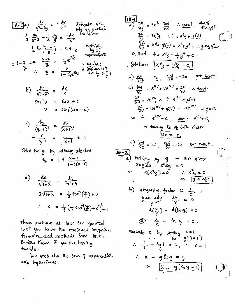


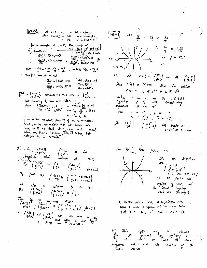


18.03 Solutions
8: Extra Problems
8A. Bifurcation Diagrams
8A-1.
a) Critical points: f (P) = 0 ⇒ P = 0, 6. See below for phase line. The integral curvesare not shown. Make sure you know how to sketch them as functions of P vs. t.
b) The picture below shows the graph of P′ = f (P) (i.e. when r = 0).A positive r will raise the graph. As soon as r > 32 the graph will have only one zero andthat zero will be above 6. Solution. r = 32.
P
JT
�
�
•0 stable
•6 semistable
Phaseline (r = 0)P' vs. P (r=0)
P
P'
6●
(2,−32)
Bifurcation
r
P
32
6
●
●
●
stable
unstable
stable
c) See above diagram. The curve of critical points is given by solving
P′ = −P3 + 12P2 − 36P + r = 0 ⇒ r = P3 − 12P2 + 36P,
which is a sideways cubic. The phase-line for r = 0 is determined by the middle plot. Thephase line for the other values of r then follow by continuity, i.e. the rP-plane is dividedinto two pieces by the curve, and arrows in the same piece have to point the same way.
8B. Frequency Response
8B-1.
a) Characteristic polynomial: p(s) = r2 + r + 7Complexified ODE: x′′ + x + 7x = F0eiωt.Particular solution (from Exp. Input Theorem): xp = F0eiωt/p(iω) = F0eiωt/(7−ω2 + iω)
Complex and real gain: g(ω) = 1/(7−ω2 + iω), g(ω) = 1/|p(iω)| = 1/√(7−ω2)2 + ω2.
For graphing we analyze the term under the square root: f (ω) = (7−ω2)2 + ω2.Critical points: f ′(ω) = −4ω(7−ω2) + 2ω = 0 ⇒ ω = 0 or ω =
√13/2.
Evaluate at the critical points: g(0) = 1/7, g(√
13/2) = .385Find regions of increase and decrease by checking values of f ′(ω):On [0,
√13/2]: f (ω) < 0 ⇒ f is decreasing ⇒ g is increasing.
On [√
13/2, ∞]: f (ω) > 0 ⇒ f is increasing ⇒ g is decreasing.

Section 8: Extra Problems 2
The graph is given below.This system has a (practical) resonant frequency = ωr =
√13/2.
b) Characteristic polynomial: p(s) = r2 + 8r + 7Complex and real gain: g(ω) = 1/p(iω) = 1/(7 − ω2 + i8ω), g(ω) = 1/|p(iω)| =1/
√(7−ω2)2 + 64ω2.
For graphing we analyze the term under the square root: f (ω) = (7−ω2)2 + 64ω2.Critical points: f ′(ω) = −4ω(7−ω2) + 128ω = 0 ⇒ ω = 0.Since there are no positive critical points the graph is strictly decreasing.Graph below.
ω
g
1 2 3 4
.1
.2
.3
.4
ωr
ωr =√
13/2
ω
g
1 2 3 4
.1
.2
.3
.4
Graphs for 8B-1a and 8B-1b.
8C. Pole Diagrams
8C-1.
a) All poles have negative real part: a, b, c, h.
b) All poles have nonzero imaginary part: b, d, e, f, h.
c) All poles are real: a, g.
d) Poles are real or complex conjugate pairs: a, b, c, g, h.
e) b, because the pole farthest to the right in b, is more negative than the one in c.
f) This is just the number of poles: a) 2, b) 2, c) 4, d) 2, e) 2, f) 4, g) 3, h) 2.
g) a) Making up a scale, the poles are -1 and -3 ⇒ P(s) = (s + 1)(s + 3) ⇒ P(D) = D2 + 4D + 3.b) Possible poles are −3± 2i ⇒ P(s) = (s + 3− 2i)(s + 3 + 2i) ⇒ P(D) = D2 + 6D + 13.c) Possible poles are −1,−3,−2 ± 2i ⇒ P(s) = (s + 1)(s + 3)(s + 2 − 2i)(s + 2 + 2i)⇒ P(D) = (D + 1)(D + 3)(D2 + 4D + 8) = D4 + 8D3 + 27D2 + 44D + 24.
h) System (h). The amplitude of the reponse is 1/|P(iω)|. In the pole diagram iωis on the imaginary axis. The poles represent values of s where 1/P(s) is infinite. Thepoles in system (h) are closer to the imaginary axis than those in system (b), so the biggest1/|P(iω)| is bigger in (h) than (b).

9. 18.03 Linear Algebra Exercises Solutions
9A. Matrix Multiplication, Rank, Echelon Form
9A-1. (i) No. The pivots have to occur in descending rows.(ii) Yes. There’s only one pivotal column, and it’s as required.(iii) Yes. There’s only one pivotal column, and it’s as required.(iv) No. The pivots have to occur in consecutive rows.(v) Yes.
9A-2 (i)[4]∼[1].
(ii) This is reduced echelon already.
(iii)
[1 11 1
]∼[1 10 0
].
(iv)
−2 1 01 −2 10 1 −2
∼1 −1
20
1 −2 10 1 −2
∼1 −1
20
0 −32
10 1 −2
∼1 −1
20
0 1 −23
0 1 −2
∼1 0 1
3
0 1 23
0 0 83
∼1 0 00 1 00 0 1
. (We’ll soon see that this is not a surprise.)
9A-3 There are many answers. For example,[1]
or[−1]
work fine. Or [ cos θ sin θ ];etc.
9A-4 Here’s several answers:
1−100
,
111−3
,
12−2−1
The interesting thing to say is that the answer is any vector in the nullspace of
[1 1 1 1
]. The simplest solution is
0000
.
9A-5 (a) The obvious answer to this question is v =
0010
; for any matrix A with
four columns, A
0010
is the third column of A.
But there are other answers: Remember, the general solution is any particular solutionplus the general solution to the homogeneous problem. The reduced echelon form of
1

A may be obtained by subracting the last row from the first row: R =
1 0 0 30 1 0 20 0 1 1
.
Rv = 0 has solutions which are multiples of
−3−2−11
. So for any t, A
1− 3t1− 2t1− t1 + t
=
101
.
(b) For any matrix with three rows, the product [ 0 0 1 ]A is its third row. In thiscase, the rows are linearly independent—the only row vector u such that uA = 0 isu = 0—so there are no other solutions.
9A-6 (a)
111
[1 0 −1]
=
1 0 −11 0 −11 0 −1
. Rank 1, as always for row × column with
both nonzero.
(b)[1 2 −1
] 111
= [2] Rank 1 just because it’s nonzero!
(c)
[1 2 00 1 1
]1 20 12 3
=
[1 42 4
]Rank 2: the columns are linearly independent (as are
the rows).
9B. Column Space, Null Space, Independence, Basis, Dimension
9B-1 First of all, any four vectors in R3 are linearly dependent. The question here ishow. The first thing to do is to make the 3× 4 matrix with these vectors as columns.Now linear relations among the columns are given by the null space of this matrix,so we want to find a nonzero element in this null space. To find one, row reduce:1 1 1 2
0 1 1 30 0 1 4
∼1 0 0 −1
0 1 1 30 0 1 4
∼1 0 0 −1
0 1 0 −10 0 1 4
The null space does’t change under these row operations, and the null space is thespace of linear relations among the columns. In the reduced echelon form it’s clearthat the first three columns are linearly independent. (This is clear from the originalmatrix, too, because the first three columns form an upper triangular matrix withnonzero entries down the diagonal.) The first three variables are pivotal, and the lastis free. Set the last one equal to 1 and solve for the first two to get a basis vector forthe null space: 1 1 1 2
0 1 1 30 0 1 4
11−41
=
0000
2

Check: the sum of the first, second, and fourth columns is 4 times the third.
9B-2 (a) Reduction steps: row exchange the top two rows, to get a pivot at upperright; then subtract twice the new top row from the bottom row.
A =
0 1 2 31 2 3 42 3 4 5
∼1 2 3 4
0 1 2 30 −1 −2 −3
∼1 0 −1 −2
0 1 2 30 0 0 0
The last transformation uses the pivot in the second row to eliminate other entries inthe second column. This is now reduced echelon.
Stop and observe: The third column is twice the second minus the first. That’s truein the original matrix as well! The fourth column is the 3 times the second minustwice the first. That’s also true in the original matrix!
Those linear relations can be expressed as matrix multiplications. The first twovariables are pivot variables and the last two are free variables. Setting x3 = 1 and
x4 = 0 and then the other way around gives the two vectors
1−210
and
2−301
, and
they form a basis for the null space of A. Any linearly independent pair of linearcombinations of them is another basis for the null space.
Similarly for AT :
AT =
0 1 21 2 32 3 43 4 5
∼
1 2 30 1 20 −1 −20 −2 −4
∼
1 0 −10 1 20 0 00 0 0
The first two variables are again pivotal, and the third is free. Set it equal to 1 and
solve for the pivotal variables to find the basis vector
1−21
. Any nonzero multiple
of this vector is another basis for the null space.
(b) We need a particular solution to
0 1 2 31 2 3 42 3 4 5
x =
111
. You could form the
augmented matrix, by adjoining
111
as a fifth column, and row reduce the result.
Maybe it’s easier to just look and see what’s there. For example the difference of the
first two columns is
111
: so xp =
−1100
works fine. Then the general solution is
3

x = xp + xh =
−1100
+ c1
1−210
+ c2
2−301
.
Then we need a particular solution to
0 1 21 2 32 3 43 4 5
x =
1111
. Again, the difference of
the first two columns works; so the general solution is x = xp+xh =
−110
+c
1−21
.
9B-3 (a) This is easy to do directly: all such vectors are multiples of
1111
, so that by
itself forms a basis of this subspace. But we can do this as directed as well. One wayto express the conditions is to say that x1 = x2, and x2 = x3, and x3 = x4. Thesethree equations can be represented by the matrix1 −1 0 0
0 1 −1 00 0 1 −1
∼1 0 −1 0
0 1 −1 00 0 1 −1
∼1 0 0 −1
0 1 0 −10 0 1 −1
The fourth variable is free, and if we set it equal to 1 we find that the other three are1 as well.
(b) A matrix representation of this relation is[1 1 1 1
]x = 0. This is already in
reduced echelon form! The first variable is pivotal, the last three are free. We find−1100
,
−1010
,
−1001
.
(c) Now there are two equations, represented by the matrix
[1 1 0 01 0 1 1
]∼[1 1 0 00 −1 1 1
]∼[
1 0 1 10 1 −1 −1
]. The first two variables are pivotal and the last two are free. A ba-
sis:
−1110
,−1101
. Looking back at the original equations, this makes sense, doesn’t
it?
9B-4 (a) If c 6= 0, there are pivots on three rows and the rank is 3. So c = 0. Therank will still be 3 unless the third row is a linear combination of the first two. The
4

first column can’t occur (because of the nonzero entries on the left), so we must haved = 2
(b) The answer is the same, since dim(Null space)+dim(Column space)=width.
9C. Determinants and Inverses
9C-1 (a) R(α)R(β) =
[cosα − sinαsinα cosα
] [cos β − sin βsin β cos β
]=
[cosα cos β − sinα sin β −(cosα sin β + sinα cos β)cosα sin β + sinα cos β cosα cos β − sinα sin β
]=
[cos(α + β) − sin(α + β)sin(α + β) cos(α + β)
]= R(α + β).
Geometrically, R(θ) rotates vectors in the plane by θ radians counterclockwise.
(b) detR(θ) = (cos θ)2 + (sin θ)2 = 1. R(θ)−1 =
[cos θ sin θ− sin θ cos θ
]= R(−θ).
9C-2 (a) det
[1 a0 1
]= 1;
[1 a0 1
]−1
=
[1 −a0 1
].
(b) det
1 a b0 1 c0 0 1
= 1 (by cross-hatch, or because the determinant of an upper-
triangular matrix is the product of the diagonal entries). To find the inverse, rowreduce1 a b 1 0 0
0 1 c 0 1 00 0 1 0 0 1
∼1 0 b− ac 1 −a 0
0 1 c 0 1 00 0 1 0 0 1
∼1 0 0 1 −a ac− b
0 1 0 0 1 −c0 0 1 0 0 1
so the inverse is
1 −a ac− b0 1 −c0 0 1
.
(c) det
0 1 11 0 11 1 0
= 2 by crosshatch. So we expect a 2 in the denominator of the
inverse.0 1 1 1 0 01 0 1 0 1 01 1 0 0 0 1
∼1 0 1 0 1 0
0 1 1 1 0 01 1 0 0 0 1
∼1 0 1 0 1 0
0 1 1 1 0 00 1 −1 0 −1 1
∼
1 0 1 0 1 00 1 1 1 0 00 0 −2 −1 −1 1
∼1 0 0 −1
212
12
0 1 0 12−1
212
0 0 1 12
12−1
2
so the inverse is 1
2
−1 1 11 −1 11 1 −1
.
5

The original matrix was symmetric. Is it an accident that the inverse is also symmet-ric?
(d) det
1 0 0 00 2 0 00 0 3 00 0 0 4
= 1 · 2 · 3 · 4 = 24. The inverse is
1 0 0 00 1
20 0
0 0 13
00 0 0 1
4
.
9D. Eigenvalues and Eigenvectors
9D-1 (a) The eigenvalues of upper or lower triangular matrices are the diagonal
entries: so for A we get 1 and 2.
[10
]is clearly an eigenvector for value 1, as is any
multiple. For λ = 2, we want a vector in the null space of A− λI =
[−1 10 0
].
[11
]or
any multiple will do nicely.
For B, the eigenvalues are 3 and 4.
[01
]is clearly an eigenvector for λ = 4, as is any
multiple. For λ = 3, we want a vector in the null space of A− λI =
[0 01 1
].
[1−1
]or
any multiple will do nicely.
(b) AB =
[4 42 8
]has characteristic polynomial pA(λ) = λ2 − (trA)λ + detA =
λ2 − 12λ+ 24 = (λ− 6)2 − (36− 24) has roots λ1,2 = 6±√
12.
(c) If Ax = λx, then (cA)x = cAx = cλx, so cλ is an eigenvalue of cA. If c = 0then cA = 0 and its only eigenvalue is 0; otherwise, this argument is reversible, sothe eigenvalues of cA are exactly c times the eigenvalues of A.
(d) A+B =
[4 11 6
]has characteristic polynomial pA(λ) = λ2−10λ+ 23 = (λ−5)2−
(25− 23) and so λ1,2 = 5±√
2.
9D-2 (a) λ2 − 2λ+ 1 = (1− λ)2.
(b) (1− λ)3.
(c) det
−λ 1 11 −λ 11 1 −λ
= (−λ)3 + 1 + 1− (−λ)− (−λ)− (−λ) = −λ3 + 3λ+ 2.
(d) (1− λ)(2− λ)(3− λ)(4− λ).
9D-3 The eigenvalue equation is
[A 00 B
]v = λv. Let’s write v =
[xy
], where x has
m components and y has n components. Then the eigenvalue equation is equivalentto the two equation Ax = λx and By = λy, for the same λ. λ is an eigenvalue if there
6

is nonzero vector satisfying this equation. This means that either x or y must benonzero. So one possiblity is that λ is an eigenvalue of A, x is a nonzero eigenvectorfor A and this eigenvalue, and y = 0. Another possibility is that λ is an eigenvalueof B, x = 0, and y is a nonzero eigenvector for B with this eigenvalue. Conclusion:
The eigenvalues of
[A 00 B
]are λ1, . . . , λm, µ1, . . . , µn.
9D-4 The eigenvalue equation is
[0 AB 0
] [xy
]= λ
[xy
]. This expands to Ay = λx
and Bx = λy. We want either x or y to be nonzero. We compute ABx = A(λy) =λAy = λ2x and BAy = Bλx) = λBx = λ2y. So if x 6= 0, then λ2 is an eigenvalue ofAB, and if y 6= 0 then λ2 is an eigenvalue of BA. Enough said.
9E. Two Dimensional Linear Dynamics
9E-1 (a) Write u =
[vw
], so u = Au with A =
[−1 11 −1
]. (Attention to signs!)
(b) A is singular (columns are proportional) so one eigenvalue is 0. The other mustbe −2 because the trace is −2.
(c) 0 has eigenvectors given by the multiples of
[11
], so one normal mode solution is
the constant solution u1 =
[11
]or any multiple. This is the steady state, with the
same number of people in both rooms. To find an eigenvector for the eigenvalue −2,
form A−λI =
[1 11 1
]; so we have
[1−1
]or any nonzero multiple. The corresponding
normal mode is u2 = e−2t
[1−1
], and the general solution is u = a
[11
]+ be−2t
[1−1
].
With u(0) =
[3010
], this gives the equations a+ b = 30, a− b = 10, or a = 20, b = 10:
so u = 20
[11
]+ 10e−2t
[1−1
]. The first term is the steady state; the second is a
transient, and it decays rapidly to zero.
When t = 1 we have v(1) = 20 + 10e−2 ∼ 21.36 and w(1) = 20− 10e−2 ∼ 18.64.
(d) When t = ∞ (so to speak), the transient has died away and the rooms haveequalized at 20 each.
9E-2 (a) This is the companion matrix for the harmonic oscillator, as explained in
LA.7, with ω = 1. The basic solutions are u1(t) =
[cos t− sin t
]and u2(t) =
[sin tcos t
], and
the general solution is a linear combination of them. A good way to think of this is toremember that the second entry is the derivative of the first, and the first can be any
7

sinusoidal function of angular frequency 1: so let’s write it as u =
[A cos(t− φ)−A sin(t− φ)
]=
A
[cos(t− φ)sin(t− φ)
].
For these to lie on the unit circle we should take A = 1. That’s it: u =
[cos(t− φ)sin(t− φ)
]for any φ. φ is both phase lag and time lag, since ω = 1. The solution goes through[10
]at t = φ.
(b) Now the characteristic polynomial is pA(λ) = λ2 − 1, so there are two real eigen-values, 1 and −1. [The phase portrait is a saddle.] Eigenvectors for 1 are killed by[−1 11 −1
]:
[11
]and multiples. The matrix is symmetric, so the eigenvectors for −1
are
[1−1
]and multiples. So the normal modes are u1 = et
[11
]and u2 = e−t
[1−1
].
The general solution is u = aet[11
]+ be−t
[1−1
].
In order for u(t0) =
[11
]for some t0, you must have aet0 = 1 and be−t0 = 0, because
the two eigenvectors are linearly independent. So b = 0, and a can be any positive
number (because you can then solve for t0): aet[11
]for a > 0. These are “ray”
solutions.
9F. Normal Modes
9F-1 The characteristic polynomial is p(s) = s4 − c. Its roots are the fourth rootsof c. Write r for the real positive fourth root of |c|. If c > 0, the fourth rootsof c are ±r and ±ir. There are four exponential solutions, but only the ones withimaginary exponent give rise to sinusoidal solutions. They are the sinusoidal functionsof angular frequency r. If c < 0, the fourth roots of c are r±1±i√
2. None of these is
purely imaginary, so there are no (nonzero) sinusoidal solutions. When c = 0 theequation is d4x
dt4= 0. The solutions are the polynomials of degree at most 3. The
constant solutions are sinusoidal.
9G. Diagonalization, Orthogonal Matrices
9G-1 The null space is (width)-(rank)=9 dimensional, so there are 9 linearly inde-pendent eigenvectors for the eigenvalue 0. There’s just one more eigenvalue, whichcan’t be zero because the sum of the eigenvalues is the trace, 5. It has to be 5.
8

9G-2 (a) A =
[1 20 3
]has eigenvalues 1 and 3. 1 has nonzero eigenvector
[10
](or any
nonzero multiple; by inspection or computation). For 3, A−3I =
[−2 20 0
]so we have
nonzero eigenvector
[11
](or any nonzero multiple). With these choices, Λ =
[1 00 3
],
S =
[1 10 1
].
B =
[1 13 3
]has eigenvectors 0 (because it’s singular) and 4 (because its trace is 4; or
by computation). An eigenvector for 0 is a vector in the null space, so e.g.
[1−1
]or any
nonzero multiple will do. For 4, A− 4I =
[−3 13 −1
]so we have nonzero eigenvector[
13
](or any nonzero multiple). With these choices, Λ =
[0 00 4
], S =
[1 1−1 3
].
(b) A3 = SΛ3S−1; to be explicit, Λ3 =
[1 00 27
].
A−1 = SΛ−1S−1; to be explicit, Λ−1 =
[1 00 1
3
].
9G-3 [The (i, j) entry in ATA is the dot product of the ith and jth columns of A.The columns form an orthonormal set exactly when this matrix of dot products isthe identity matrix.]
A =
[−2 11 −2
]has characteristic polynomial pA(λ) = λ2 + 4λ + 3 = (λ + 1)(λ + 3),
so eigenvalues −1 and −3 and Λ =
[−1 00 −3
]. Eigenvectors for 1 are killed by
A− I =
[−1 11 −1
]; so
[11
]or any nonzero multiple. We could find an eigenvector for
3 similarly, or just remember that eigenvectors for distinct eigenvalues of a symmetric
matrix are orthogonal, and write down
[1−1
]. Each of these vectors has length
√2,
so an orthogonal S is given by S = 1√2
[1 11 −1
].
(There are seven other correct answers; one could list the eigenvalues in the oppositeorder, and change the signs of the eigenvectors.)
9H. Decoupling
9H-1 The rabbit matrix is A =
[3 12 4
]. We found eigenvalues 2, 5 and eigenvector
9

matrix S =
[1 1−1 2
], with inverse S−1 = 1
3
[2 −11 1
]. The decoupling coordinates are
the entries in y such that Sy = x, or y = S−1x = 13
[2x1 − x2
x1 + x2
]: y1 = 2x1 − x2 (for
eigenvalue 2) and y2 = x1 + x2 (for eigenvalue 5), or any nonzero multiples of these,do the trick. y1(t) = e2ty1(0), y2(t) = e5ty2(0). y2(t) is the sum of the populations,and it grows exponentially with rate 5, just as if there was no hedge.
9I. Matrix Exponential
9I-1 By time invariance the answer will be the same for any t0; for example we could
take t0 = 0; so
[x(t0 + 1)y(t0 + 1)
]= eA
[x(t0)y(t0)
]. Then we need to compute the exponential
matrix. We recalled the diagonalization of the rabbit matrix above, so eAt = SeΛtS−1,
and eA =
[3 12 4
] [e2 00 e5
]1
3
[2 −11 1
].
9I-2 pA(λ) = λ2 + 2λ+ 2 = (λ+ 1)2 + 1 has roots −1± i. Eigenvectors for λ = −1 + i
are killed by A− (−1 + i)I =
[1− i 1−2 −1− i
]; for example
[−1
1− i
]. The exponential
solutions are e(−1+i)t
[−1
1− i
]and its complex conjugate, so we get real solutions as
real and imaginary parts, which we put into the columns in a fundamental matrix:
Φ(t) = e−t[− cos t − sin t
cos t+ sin t − cos t+ sin t
]
Φ(0) =
[−1 01 −1
], Φ(0)−1 = −
[1 01 1
],
eAt = Φ(t)Φ(0)−1 = e−t[cos t+ sin t sin t−2 sin t cos t− sin t
]
9J. Inhomogeneous Solutions
9J-1
(a) As always, substitution of up = e2tv gives the exponential response formula
v =
[−4 −5−1 0
]−1 [12
]= −1
5
[10−7
]⇒ up = −1
5e2t
[10−7
].
10

(b) Complex replacement and the trial solution zp = e2itv gives
v =
[2i− 1 0−1 2i− 2
]−1 [10
]=
1
−2− 6i
[2i− 2
1
]=
1
20
[−4− 8i−1 + 3i
]So
zp =1
20(cos(2t) + i sin(2t))
[−4− 8i−1 + 3i
]=
1
20
([−4 cos(2t) + 8 sin(2t)− cos(2t)− 3 sin(2t)
]+ i
[−4 sin(2t)− 8 cos(2t)− sin(2t) + 3 cos(2t)
])Therefore
up = Re (zp) =1
20
[−4 cos(2t) + 8 sin(2t)− cos(2t)− 3 sin(2t)
]
9J-2 We want to compute a particular solution to x = Ax+
[−et0
], using x(t) = Φ(t)
∫Φ(t)−1
[−et0
]dt.
Φ(t) = SeΛt, so Φ(t)−1 = e−ΛtS−1. S−1
[−et0
]= −1
3et[21
].
Φ(t)−1
[−et0
]= e−ΛtS−1
[−et0
]= −1
3
[e−2t 0
0 e−5t
]et[21
]= −1
3
[2e−t
e−4t
].∫
Φ(t)−1
[−et0
]dt =
1
3
[2e−t14e−4t
].
x(t) = Φ(t)1
3
[2e−t14e−4t
]=
1
3S
[e2t 00 e5t
] [2e−t14e−4t
]=
1
12etS
[81
]=et
12
[1 1−1 2
] [81
]=et
4
[3−2
].
We still need to get the initial condition right. We need a solution to the homogeneous
equation with inital value1
4
[12
]. Luckily, this is an eigenvector, for value 5, so the
relevant solution ise5t
4
[12
], and the solution we seek is
et
4
[3−2
]+e5t
4
[12
].
11

10. 18.03 PDE Exercises Solutions
10A. Heat Equation; Separation of Variables
10A-1 (i) Trying a solution u(x, t) = v(x)w(t) leads to separated solutions uk(x, t) =vk(x)wk(t) where vk(x) = sin(πkx), and wk(t) = e−2π
2k2t, and k = 0, 1, 2, . . ..
(ii) u(x, 0) = 2π
∑∞k=1
(−1)k+1
ksin(πkx)
(iii) u(x, t) = 2π
∑∞k=1
(−1)k+1
ksin(πkx)e−π
2k2t
(iv) u(12, 1) ≈ .00032
10A-2 (i) Separated solutions uk(x, t) = vk(x)wk(t) where vk(x) = sin(πkx), andwk(t) = e−2π
2k2t (Note factor of 2 from (10A-2.1)) and k = 0, 1, 2, . . .
(ii) u(x, 0) = 4π
∑k odd
sin(πkx)k
(iii) u(x, t) = 4π
∑k odd
sin(πkx)k
e−2π2k2t
10A-3 (a) ust(x, t) = U(x) = 1 − x
(b) Since the heat equation is linear u satisfies the PDE (10A-3.1). At the boundary(x = 0 and x = 1) we have u(0, t) = u(0, 1) − ust(0, t) = 1 − 1 = 0. Likewiseu(1, t) = 0. That is, u is a solution to the heat equation with homogeneous boundaryconditions in 10A-1. The initial condition is u(x, 0) = x. We found the coefficientsfor this in 10A-1.
u(x, t) =2
π
∞∑k=1
(−1)k+1
ksin(πkx)e−2π
2k2t.
(c)
u(x, t) = U(x) + u(x, t) = 1 − x+2
π
∞∑k=1
(−1)k+1
ksin(πkx)e−2π
2k2t.
(d) u(x, t)−U(x) = u(x, t) The term in the sum for u that decays the slowest is whenk = 1. Therefore we need 2
πe−2π
2T = .01U(1/2) = .005. Solving we get T = .246
10B. Wave Equation
10B-1 (a) Separating variables, we look for a solutions of the form u(x, t) = v(x)w(t),which leads to v′′(x) = λv(x) with v(0) = v(π/2) = 0, and hence
vk(x) = sin(2kx)
Consequently, wk = −(2k)2c2wk, whic implies
wk(t) = A cos(2ckt) +B sin(2ckt)
1

The normal modes are
uk(x, t) = sin(2kx)(A cos(2ckt) +B sin(2ckt)),
where A and B must be specified by an initial position and velocity of the string.
(b) The main note (from the mode u1) has frequency2c
2π=c
π. You will also hear the
higher harmonics at the frequenciesck
π, k = 2, 3, . . . . (The sound waves induced by
the vibrating string depend on the frequency in t of the modes.)
(c) Longer strings have lower frequencies, lower notes, and shorter strings have higherfrequencies, higher notes. If the length of the string is L, then the equations v′′(x) =λv(x), v(0) = v(L) = 0 lead to solutions vk(x) = sin(kπx/L). (In part (a), L = π/2.)The associated angular frequencies in the t variable are kcπ/L, so the larger L, thesmaller kcπ/L and the lower the note. Thus c is inversely proportional to the lengthof the string.
(d) When you tighten the string, the notes get higher, and the frequency you hear isincreased. (Tightening the string increases the tension in the string and increases thespring constant, which corresponds to c. The frequencies of the sounds are directlyproportional to c.)
2

M.I.T. 18.03 Ordinary Differential Equations18.03 Notes and Exercises
c©Arthur Mattuck, Haynes Miller, David Jerison, Jennifer French, JeremyOrloff and M.I.T. 2007, 2013, 2017
1