misvaluing innovation* - hbs people spacemisvaluing innovation — page 1 firms engage in a...

Misvaluing Innovation*

Lauren Cohen

Harvard Business School and NBER [email protected]

Karl Diether

Tuck School of Business at Dartmouth College [email protected]

Christopher Malloy

Harvard Business School and NBER [email protected]

First Draft: November 2010

This Draft: July 2012

* We would like to thank Brad Barber, James Choi, Andrea Frazzini, Ken French, Robin Greenwood, Keith Gamble, Umit Gurun, Cam Harvey, Byoung-Hyoun Hwang, Harrison Hong, Mike Lemmon, Dong Lou, David Solomon, Laura Starks, Jeremy Stein, Tuomo Vuolteenaho, an anonymous referee, and seminar participants at Analysis Group, Arrowstreet Capital, Columbia University, Dartmouth College, DePaul University, Luxembourg School of Finance, Nova School of Business and Economics, Rice University, the Rodney White Center conference on Household Portfolio Choice and Investment Decisions at University of Pennsylvania Wharton School, the University of Miami Behavioral Finance Conference, the Nomura Global Equity Conference in London, and the AFA Meetings in Chicago for helpful comments and suggestions. We are grateful for funding from the National Science Foundation.

ABSTRACT We demonstrate that a firm’s ability to innovate is predictable, persistent, and relatively simple to compute, and yet the stock market ignores the implications of past successes when valuing future innovation. We show that two firms that invest the exact same in research and development (R&D) can have quite divergent, but predictably divergent, future paths. Our approach is based on the simple premise that while future outcomes associated with R&D investment are uncertain, the past track records of firms may give insight into their potential for future success. We show that a long-short portfolio strategy that takes advantage of the information in past track records earns abnormal returns of roughly 11 percent per year. Importantly, these past track records also predict divergent future real outcomes in patents, patent citations, and new product innovations.

Misvaluing Innovation — Page 1

Firms engage in a variety of activities. Some of these activities are straightforward, and

easy to assess how they will impact firm value (e.g., maintenance capital expenditures).

However, some of these activities, while crucially important for the discounted value of a

firm’s future cash flows, are quite uncertain and difficult to decipher how they will

ultimately impact firm value. Although hard to assess, it may still be the case that

analysis of publicly available information can give substantive insight into reducing the

uncertainty surrounding these actions.

The activity at the heart of our investigation is investment in research and

development (R&D). Given that R&D stimulates innovation and technological change,

which can in turn lead to improvements in productivity, living standards, and

economic output, the proper allocation of R&D investment in the economy is a critical

task of the market. And yet, this task is made difficult by the fact that R&D investment

is such a highly uncertain activity. Perhaps as a result of this uncertainty, R&D

investment has increasingly become a market-driven activity. Although the share of

R&D as a percentage of GDP has remained roughly constant (between 2-3%) since the

1960s, the composition of R&D investment in the economy has shifted dramatically, away

from federal spending and toward private sector spending.1 Since the late 1980s, for

example, virtually all of the increases in total R&D spending have come from the private

sector. The market’s role in allocating R&D investment has become more important

than ever.

In this paper we demonstrate that the stock market is unable to distinguish

between “good” and “bad” R&D investment, despite the fact that successful innovation

is in fact predictable. We show that two firms that invest the same amount in R&D can

have quite divergent, but predictably divergent, future paths. Our approach is based on

the simple premise that while future outcomes associated with R&D investment are

uncertain, past information about firms’ success at R&D gives us insight into their

potential for future success.

Our empirical strategy proceeds from the notion that past track records represent

one simple way to gauge the future prospects of firms. Some firms are skilled at certain

activities, and some are not, and this skill may be persistent over time. Using this idea

1 See Congressional Budget Office’s 2005 report entitled “R&D and Productivity Growth.”


as the starting point for our analysis, we examine the predictability of firm-level R&D

investment track records for future returns and future real outcomes. We find that

although R&D success is predictable, persistent, and relatively simple to compute, the

market largely ignores the information embedded in past track records.

Our identification of past R&D success is based on a simple framework of using a

firm’s past ability in translating R&D into something the firm values. We then take this

“ability” of a firm at R&D and interact it with the amount of research the firm is

actually undertaking. For instance, we examine the outcomes of those firms that have

been quite good at R&D and are investing heavily in R&D with firms investing identical

amounts in R&D, but that have poor past track records. If the market correctly takes

into account the prior track records’ implications for future success, then whether firms

are optimally choosing levels of R&D or not, the market should impound relevant

information regarding innovation into prices. In fact, the market could even be

completely incorrect in impounding the impact of every firm’s R&D expenditures (as they

do have uncertain effects on future firm value), but this would still have no implication

for predictability based on past information, as the market will sometimes overvalue and

sometimes undervalue this innovation.

We find that the market consistently misvalues innovation in an ex-ante,

predictable way. Specifically, the market does not take into account the information in

firms’ past R&D abilities. Firms that have been successful in the past and that invest

heavily in R&D as a percentage of sales (“GoodR&D” firms) earn substantially higher

future stock returns than firms that invest identical amounts in R&D, but that have poor

past track records (“BadR&D” firms). A portfolio of GoodR&D firms earns equal- and

value-weighted excess returns of 135 basis points per month (t=2.76) and 122 basis points

per month (t=2.61), and 4-factor alphas of 90 basis points per month (t=3.11) and 78

basis points per month (t=2.27), respectively. In contrast, the portfolio of firms with

poor past track records but that invests the same amount of R&D (BadR&D) earns -15

basis points per month in 4-factor value-weighted alpha (t=0.56). The spread portfolio

that takes identical high R&D-level portfolios, but exploits differences in past track

records, has a 4-factor alpha of 93 basis points per month (t=2.30) or over 11% per year.

Returns to the “GoodR&D” (and spread) portfolios are large and significant in the first


year, and then returns remain slightly positive but basically plateau in the second and

third years, with no reversal. This suggests that we are not capturing a form of

overreaction, but instead that the embedded information regarding innovation that the

market is misvaluing is important for fundamental firm value.

Our findings add to a growing literature highlighting the market’s inability to

properly value investments in R&D. On one hand, some researchers argue that investors

may overestimate the benefits from R&D or simply ignore the fact that many R&D

investments are not profitable (Jensen (1993)), leading to the overpricing of R&D-

intensive firms. For example, Lakonishok, Shleifer, and Vishny (1994) find that growth

stocks earn low future returns, while Daniel and Titman (2006) show that this growth

stock underperformance is concentrated in stocks with significant “intangible”

information, consistent with market overreaction to intangible information that is

difficult to interpret.2 However, the recent evidence on firm-level R&D activity suggests

that, if anything, the market appears to underreact to the information contained in R&D

investments. For example, Chan, Lakonishok, and Sougiannis (2001) and Lev and

Sougiannis (1996) demonstrate that firms with high ratios of R&D relative to market

equity earn high subsequent returns; Eberhart et al. (2004) find that large increases in

R&D expenditures predict positive future abnormal returns; and Hirshleifer et al. (2010)

show that firm-level innovative “efficiency” (measured as patents scaled by R&D)

forecasts future returns.3 We show that our results are unaffected by the inclusion of

these measures in our tests, and are roughly 3 times larger in magnitude than the findings

in, for example, Eberhart et al. (2004) and Hirshleifer et al. (2010), suggesting that our

approach is picking up a new and previously undetected pattern in the cross-section of

stock returns associated with the market’s misvaluation of high R&D ability firms.

To combat the concern that our results are due to data mining, we run a series of

out-of-sample tests on our findings. We find that our classification of high ability R&D

firms is also predictive of future returns in an international sample (including the UK,

Japan, and Germany) and in the period immediately preceding our sample period (1974-

2 See also Daniel, Hirshleifer, and Subrahmanyam (1998, DHS)’s distinction between public and private information. DHS theorize that investors are overconfident about the precision of their private signals, and therefore overreact to intangible private information and underreact to tangible public information. 3 See also Porter (1992), Hall (1993a), and Hall and Hall (1993), who argue that investors may be myopic and discount the cash flows from R&D capital at a very high rate, leading to underpricing.


1980). For example, when we employ our baseline Fama-MacBeth cross-sectional

regression on an international sample that pools together the universe of stocks from the

UK, Japan, and Germany (using dollar-returns on all stocks), we find a coefficient on

R&Dhigh*abilityhigh of 0.501 (t=2.24), which is similar in magnitude and significance to our

U.S. findings. In addition, while our baseline U.S. portfolio results are driven by a small

number of firms (the High Ability-High R&D portfolio described above contains an

average of 10 stocks per month), the percentage of market capitalization in the portfolio

(0.71% of the stock market’s annual value on average) is larger than that of the “small

value” portfolio (0.50% of the stock market’s annual value on average) that is featured in

hundreds of asset pricing papers, and which remains one of the most studied anomalies in

the literature.

Lastly, we run a series of tests designed to pinpoint the mechanism behind our

results. First, we explore real outcomes associated with our high R&D ability firms.

Specifically, we show that the firms that we classify as high ability firms and that invest

heavily in R&D also produce tangible results with their research and development efforts.

They generate significantly more patents, achieve significantly more patent-citations, and

develop significantly more new products than firms that invest the same levels of R&D,

but have poor track records. In addition, we demonstrate that high ability firms exhibit

significant persistence in R&D skill, that this skill may be positively related to the

presence of a founder, and that the market’s failure to understand the implications of

R&D track records is related to heterogeneity in information provision by firms. For

example, we show that the predictability in future returns is significantly lower for high

ability firms who provide more earnings guidance; under the assumption that firms that

provide more earnings guidance are also likely to provide more information to investors

more generally (as in Jones (2007)), these findings suggest that cross-sectional variation

in information opacity may help explain why the market fails to properly understand the

information embedded in firms’ past track records.

I. Data and Summary Statistics

We combine a variety of data sources to create the sample we use in this paper.

We draw monthly stock returns, shares outstanding, and volume capitalization from


CRSP, and extract a host of firm-specific accounting variables, such as research and

development (R&D) expenditures, sales and general administrative expenses (SG&A),

book equity, etc., from Compustat. We combine these items with firm-level patent data

drawn from the NBER’s U.S. Patent Citations Data File,4 segment-level product data

from the Compustat Segment Data File, earnings’ guidance data from First Call and

CEO founder data from Fahlenbrach’s (2009) hand-collected data and the Corporate

Data Library. We draw international stock return data from Datastream and accounting

data from Worldscope. We filter the datastream stock return data and identify common

stocks using the procedures and suggestions outlined in Ince and Porter (2006) and

Griffin, Nadari, and Kelly (2010).

Table I presents summary statistics for the sample we use in this paper (Panel B),

compared to the entire universe of stocks on CRSP (Panel A), over our July 1980 to

December 2009 sample period. Our sample includes all NYSE, AMEX, and Nasdaq

common stocks (CRSP share code 10-12) with a valid (i.e., non-missing) R&D estimate in

a given year, as well as a valid estimate for the "Ability" measure that features in our

analysis.

The notion of “Ability” is meant to capture simply how good a firm is at turning

R&D expenditures into something the firm values. We have run our tests using a

number of measures of what the firm “values” and our results are robust to the various

measures we have tried. The measure we show in the paper is how R&D translates into

actual future sales revenue of the firm.5 One additional concern may be the horizon we

use to identify the translated effect of R&D on future outcomes. As we describe below,

we try to be flexible on this dimension and use up to a five-year lag in measuring the

impact of past R&D expenditures on future firm outcomes.

Thus, for sales (reported in the paper), we compute firm “Ability” by running

rolling firm-by-firm regressions of firm-level sales growth (defined as log(Salest/Salest-1))

on lagged R&D (R&Dt-j/Salest-j; where j=1,2,3,4,5). We run separate regressions for 5

4 The patent data is collected, maintained, and provided by the National Bureau of Economic Research Patent Data Project. All data files we use, along with documentation, can be obtained from the project’s website at https://sites.google.com/site/patentdataproject/Home. 5 As mentioned, we have used various measures of profitability, such as return-on-assets (ROA), instead of sales growth. The results are very similar in magnitude and significance. For instance, the analog of the Spread portfolios from Table III using ROA have monthly 3- and 4-factor alphas of 51 and 59 basis points (t=2.10 and 2.39), respectively.


different lags of R&D (i.e., R&D from years t-1, t-2, t-3, t-4, and t-5); we then take the

average of these five R&D regression coefficients as our measure of ability (regression

specification shown in Table II). Again, the idea behind this measure is to isolate the

extent to which a given firm successfully converts its R&D investments into future sales.

We have analyzed a variety of different specifications here, and our results are robust to

these permutations; for example, running a single regression for each firm of sales growth

on the average of the past 5 years of R&D, and using this single coefficient as our

measure of ability yields similar, and often stronger, results (we show these results in

Appendix Table A5).

In estimating a firm’s ability, for every firm in each year we use 8 years of past

data for each firm-level regression, and we then run these regressions on a rolling basis

each year using the prior 8 years of data. For each regression, we require a minimum of

6 (75%) non-missing R&D observations and that at least half the R&D observations are

non-zero; otherwise, we set the slope coefficients to missing values.6 Panel B of Table I

indicates that our final sample is quite similar to the overall sample of CRSP stocks.

Comparing characteristic-by-characteristic, our sample does contain slightly larger stocks,

with a modest growth tilt relative to the overall sample of CRSP stocks. While the stocks

in our sample are slightly less levered, the price momentum, turnover, and stock volatility

are nearly identical to the entire universe. Overall, the differences between the two

samples appear small.

Panel A of Table II presents the full-sample sample averages of the rolling firm-by-

firm regression coefficients that form the basis of our ability measure. The average

ability estimate is 3.33, with an average sales growth of roughly 7%, while average R&D

expenditures equate to roughly 17% of sales.

We then turn to some diagnostics of our Ability measure. If we are truly

capturing a meaningful measure of a firm’s ability at Research and Development, we

6 We have analyzed back-windows of 6-10 years of past data as well, with the trade-off coming between fewer data points required (so more observations estimated) per firm, but less reliable estimates, compared with, say requiring 10 years of data, which allows fewer observations to be estimated (and more auto-correlated estimates as only 1 observation changes per estimation period), but more precise estimates. We choose the mid-point of using 8 years of past data. The results look very similar across these estimation windows, in magnitude and significance. In fact, in magnitude the results for both 6- and 10-year windows are a bit larger (for instance the value-weighted Spread portfolio using a 10-year back window has 4-factor alpha abnormal returns of 101 basis points per month (t=2.49) as opposed to the 93 basis points reported in Table III).


might expect to see some level of persistence in this measure (i.e., it would be odd to see

firms simply jump from being classified as “good” at R&D to “poor” at R&D, and back,

year after year). Panel B of Table II examines this issue by showing the annual

persistence in a firm’s ability quintile assignment, for yearly lags out to 5 years. We find

that firms in the highest quintile of ability remain in this same top quintile in the

following year 70% of the time.7 Overall, Panel B demonstrates that there is substantial

persistence in firm-level R&D ability, but that firms do transition out (on average) of the

high ability category within several years.8

II. Results

A. Portfolio Returns

In this section we examine average returns on portfolios formed using information

about both a firm’s ability and its level of R&D. We scale R&D by sales, and use three-

way sorts using the same methodology of Fama and French (1996), namely: R&Dlow

contains all stocks below the 30th percentile in R&D (but who have R&D greater than

zero), and R&Dhigh contains all stocks above the 70th percentile in R&D. We compute

firm-year ability as described earlier, using the annual average of the rolling regression

coefficients of sales growth on 5 lags of R&D (scaled by sales).9 We include all NYSE,

7 To construct a baseline to compare this 70% against, we simulate our data using the parameters of our data (i.e., assuming a world with the exact same number of firms, and using the same rolling windows for these firms), but with R&D and sales replaced with standard normal variables. We run 1,000 simulations, and the averages of the 1,000 simulations are reported in the Internet Appendix Table A1. Comparing this simulated ability measure’s persistence to the actual data, the 70% persistence in our high ability quintile is significantly higher than would be expected by chance: e.g., the Monte Carlo simulation results in Appendix Table A1 indicate that one should expect a firm in the top quintile to remain in the top quintile in the following year only 54% of the time; thus the 70% persistence of our actual ability measure is roughly 30% larger in magnitude than the simulated persistence expected by chance. 8 This level of persistence stands in contrast to the lack of persistence shown in the mutual fund performance literature (see, for example, Brown, Goetzmann, Ibbotson, and Ross (1992), Malkiel (1995), Wermers (1997), Carhart (1997), and Daniel et al. (1997)) and the modest persistence shown in the hedge fund performance literature (see, for example, Agarwal and Nail (2000, 2004), Fung, Hsieh, Nail, and Ramadorai (2008), Kosowski, Nail, and Teo (2007), and Teo (2011)). 9 In order to further test the robustness of our measure, we perform a number of falsification exercises. First, if we replace R&D with a non-negative random variable with the same time-series mean and stand deviation as the typical stock’s R&D in the sample (keeping every other aspect of the sample the same), we find virtually no spread in returns. Also, if we just remove R&D from the ability estimation altogether (and simply use 1/sales instead), we again find no spread in returns. Finally, if we use raw R&D when estimating ability instead of scaled R&D, we still find significant (although slightly smaller) portfolio spreads (=43 basis points, t=1.81). These results indicate that our findings are not driven by our choice of


AMEX, and Nasdaq stocks from July 1978 to December 2009 with lagged share prices

above $5 into these portfolios, and rebalance the portfolios yearly.

We characteristically-adjust returns (as in Daniel et al. (1997)) using either 25

size/book-to-market benchmark portfolios, or 125 (5x5x5) size/book-to-

market/momentum benchmark portfolios. We also compute three- and four-factor alphas

(as in Fama and French (1996), and Carhart (1997)) by running time-series regressions of

excess portfolio returns on the market (MKT), size (SMB), value (HML), and momentum

(UMD) factor returns. In addition to these risk adjustments, we also calculate an

industry benchmark-adjusted return. If the ability measure is somehow sorting on

industry (so the High Ability firms are disproportionately from one industry), we may be

inadvertently sorting on an industry characteristic unrelated to our ability explanation.

To combat this potential problem, each month we compute each firm’s return subtracting

out its industry’s return over the same month. Thus, these industry excess returns will

control for any characteristic of a firm (High or Low Ability) shared by its industry, and

isolate only its abnormal returns relative to other firms in the same industry.10 Lastly, as

we will compare the returns of two firms that have both been spending a large amount on

R&D (but with varying abilities), we have no selection bias in terms of firms that decide

to engage (or not) in R&D. This also rules out any general story that there has been an

unexpected positive trend for innovative firms over the past 30 years, as that would show

up in all high R&D firms. Equivalently, we compare the returns within High Ability

firms, varying levels of R&D, to rule out the possibility of High Ability sorting an

unobserved risk.

Table III reports average stock returns for monthly portfolio sorts, and illustrates

our first main result: stocks that exhibit high ability in the past and that spend a large

amount on R&D (i.e., stocks in the Abilityhigh / R&Dhigh portfolio, which we will call the

"GoodR&D" portfolio) outperform in the future. This result holds for both equal- and

value-weight portfolio returns, and for excess returns, characteristically-adjusted returns,

industry-adjusted returns, and 3- and 4-factor alphas. Further, the magnitude of this

outperformance is large: Panel A shows that the GoodR&D portfolio earns 135 basis

scaling variable, but instead suggest we are capturing an important aspect of R&D spending. 10 We assign firms into 17 industries, as defined in Fama and French (1997). Running it using the 10-, 12-, 30-, or 49-industry defined portfolios has no effect on the magnitude or significance of the results.


points per month (t=2.76) in equal-weight excess returns, and 122 basis points per month

(t=2.61) in value-weight excess returns, which translates to 17.5% and 15.7% annually,

respectively. In addition, the long-short portfolio spread (Spread) between stocks in the

GoodR&D portfolio and those stocks that exhibit low ability in the past but which

continue to spend a large amount on R&D (i.e., stocks in the Abilitylow / R&Dhigh

portfolio, which we will call the "BadR&D" portfolio), is large and significant. For

example, Panels A and B shows that the raw equal-weight spread is 73 basis points per

month (t=2.61), and the raw value-weight spread is 90 basis points per month (t=2.30),

which translates to 9.1% and 11.4% annually, respectively. Again this result holds for

both equal- and value-weight portfolio returns, and for characteristically-adjusted returns,

industry-adjusted returns, and 3- and 4-factor alphas. Note that the two components of

this spread portfolio (i.e., the GoodR&D portfolio vs. the BadR&D portfolio) are very

similar on other characteristics (e.g., in percentiles, the average size (0.46 vs. 0.43), book-

to-market (0.31 vs. 0.38), leverage (0.26 vs. 0.25), momentum (0.56 vs. 0.53), volatility

(0.53 vs. 0.49), turnover (0.72 vs. 0.69), and past R&D growth (0.65 vs. 0.69) are

virtually the same for both portfolios).

Panel C of Table III presents additional characteristics of these portfolios.

Specifically, the four-factor loadings in Panel C suggest that the GoodR&D portfolio

loads negatively on value and momentum and positively on size, meaning that the stocks

in this portfolio are typically large, growth stocks with poor past returns. Meanwhile the

spread portfolio has no significant loadings on any of the four factors, indicating that the

returns to this portfolio do not covary with any of these well-known factors. In addition,

while Panel C reveals that the High Ability-High R&D portfolio contains an average of

only 10 stocks per month, the percentage of combined market capitalization in this

portfolio (0.71% of the stock market’s annual value on average) is larger than that of the

“small value” portfolio (0.50% of the stock market’s annual value on average) that is

featured prominently in the literature.

The results here are not sensitive to the particular breakpoints chosen; sorting

based on quintiles or quartiles produces very similar (sometimes even a bit stronger)

results. For example, the equal-weighted DGTW characteristically adjusted-spread

return using 5x5 sorts is 120 basis points per month (t=2.29), while Appendix Tables A4


show that this same spread return using 4x4 sorts is 95 basis points per month (t=3.57).

We have additionally tried coarser sorts, as in Appendix Table A3, where we simply split

by median level of R&D. These sorts, while having less power to distinguish between

R&D spending levels, again yield the same result: High Ability firms that engage in more

R&D spending outperform Low Ability firms that also are above median spenders on

R&D. The analogous DGTW spread portfolio returns 55 basis points per month

(t=3.70). Further, the High Ability-High R&D contains an average of 29 stocks per

month, with an average market capitalization of 1.93%. This is larger than the combined

market capitalization of value quintile portfolios #1-3 (which together account for 1.71%

[=0.50+0.49+0.72] of total market capitalization on average, and which collectively

account for most (80%) of the value premium from 1963-2009).11 Lastly, we also present

results in Appendix Table A9 using “conditional sorts” (as opposed to the independent

sorts we use for most of the paper) which sort stocks based on Ability, and *then* by

R&D within each Ability bin. This approach forces the number of stocks to be equal in

each portfolio bin, and by doing so increases the number of stocks in the “High-High”

portfolio. Appendix Table A9 shows that for 5x5, 4x4, and 3x3 conditional sorts, the

number of stocks in this portfolio increases significantly (up to 74 stocks per month), and

our results remain robustly large and significant.

It is also important to note here that firms only report R&D expenses once per

year, and we only calculate Ability once per year. Thus, although we report monthly

returns in this table, we only rebalance our portfolios once per year.

We also find virtually no reversal of the abnormal returns we document here.

Panel A of Figure 1 plots the spread portfolio (GoodR&D-BadR&D) of Cumulative

Abnormal Returns (CARs) following portfolio formation at time 0 through the first

eighteen months, and Panel B plots the GoodR&D portfolio. Both equal- and value-

weighted CARs are shown, which are the size-BM-momentum-adjusted returns each

month. Returns of the spread (and GoodR&D) portfolios are large and significant in the

first year (documented in Table IV), and then returns drift up slightly but basically

11 This 1.93% is also larger than the combined market share of the “Loser portfolio” (Decile 1) from the momentum anomaly (Jegadeesh and Titman (1993)), which comprises an average of 1.81% of total market capitalization each year, and accounts for roughly two-thirds (65%) of the profits to the (Winner-Loser) momentum strategy.


plateau. Importantly, even continuing on into the second and third years, there is no

reversal in returns. This suggests that we are not capturing a form of overreaction, but

instead that the embedded information about innovation that the market is misvaluing is

important for fundamental firm value.

Figure 2 graphs the equal-weight yearly returns to the spread portfolio.12 Figure 2

shows that the annual returns to the strategy are fairly stable across time, and the

average annual return to the spread portfolio across the 29 years in our sample is 10.8%

(t=2.29). In Appendix Table A2 we also split our sample into three distinct sub-periods,

and show that no single sub-period drives our results. For example, the value-weight L/S

spread is 46 basis points per month (t=1.01) in the 1980s, 115 basis points per month

(t=2.45) in the 1990s, and 142 basis points per month (t=1.85) in the 2000s; the equal-

weight equivalents are 25 basis points per month (t=0.55) in the 1980s, 121 basis points

per month (t=3.67) in the 1990s, and 135 basis points per month (t=2.78) in the 2000s.

Further, the annual correlation of these spread portfolio returns with the excess market

return is low: 0.29 for the equal-weight, and 0.11 for the value-weight.13

In Table IV we demonstrate that simple sorts on R&D or Ability alone yield no

pattern in average returns. In Panel A, we present monthly portfolio returns for quintiles

based on R&D (scaled by sales).14 We group stocks with no R&D (R&Dzero) into a

separate portfolio.15 Panel A indicates that excess returns across the various groups are

very similar, and that the spread in returns between R&Dhigh and R&Dlow, and also

between R&Dhigh and R&Dzero are small and insignificant. We also characteristically-

adjust returns (as in Daniel et al. (1997)) using 125 value-weight size/book-to-

market/momentum benchmark portfolios. Again we see no pattern in the abnormal

return spreads of portfolios sorted on R&D. Note that these results are not sensitive to

the particular breakpoints chosen, to the particular risk-adjustment procedure employed,

or to the particular scaling variables used (except for market equity, of course, which

12 The analogous value-weight version of this figure can be found in the Appendix, as Figure A1. 13 Monthly return correlations with the monthly excess market return are even lower: 0.09 for the equal-weight and 0.03 for the value-weight. 14 The results are the same if we use the three-way sorts used in Table III. 15 We separate out the R&Dzero to show any differences that may arise in this portfolio (as these make up roughly 25% of the firms that report R&D). Table IV shows that these stocks do not have significantly different returns. Further, including these in the interaction (or excluding them) does not materially affect the results (i.e., Table V actually does this comparison in Columns 3 and 4, and the results are nearly identical in magnitude and significance).


mechanically produces a scaled price effect when used as a denominator irrespective of

numerator (see Fama and French (1996)).

Panel B of Table IV presents the average monthly portfolio returns associated

with simple sorts on our ability measure. As with the simple sorts on R&D, these sorts

on ability yield no obvious pattern in excess returns or abnormal returns, and the spread

between Abilityhigh and Abilitylow is always near zero and insignificant. Lastly, the

correlation of R&D and Ability is -0.04. In other words, they seem to be picking up quite

different information about firms.16

In summary, the results in Tables III and IV demonstrate that our simple

classification scheme, which is designed to isolate high-ability firms solely based on their

past success in converting R&D into future sales, produces a large spread in future

abnormal returns that is not present when looking at simple sorts on R&D, or simple

sorts on ability alone. This finding highlights the fact that even though two firms may

spend an equal amount on research and development, it is critical to understand the

likely effectiveness of these expenditures, and that one can estimate this effectiveness by

simply looking at a firm’s past experience. Thus our approach offers an ex-ante method

for identifying future innovation that is likely to be successful, which we show is in fact

the case in Section III.

B. Cross-Sectional Regressions

Our next set of tests employ monthly Fama and Macbeth (1973) cross-sectional

regressions each month to further assess the predictive power of our ability classification.

To control for the well-known effects of size (Banz (1981)), book-to-market ((Rosenberg.

Reid, and Lanstein (1985), Fama and French (1992)), and momentum (Jegadeesh and

Titman (1993), Carhart (1997)), we include controls for these as independent variables.

Additionally, we include controls on the right-hand side for one-month past returns (to

capture the liquidity and microstructure effects documented by Jegadeesh (1990)),

volume (the average daily share turnover during the previous 12 months), and return

volatility (the standard deviation of daily returns over the previous 12 months). Lastly,

16 We have also calculated the correlation of the R&Dhigh and Abilityhigh categorical variables, which is -0.25, again suggesting that neither heavily investing in R&D, nor having a high Ability using this measure, implies much about the other.


we include industry fixed effects to control for any industry level characteristic that may

be driving our results. Our variable of interest is the interaction between our measure of

high ability (Abilityhigh) and R&D. Analogous to Table IV, Abilityhigh is a dummy

vsriable equal to one for stocks in the highest quintile of ability each year, and zero

otherwise. We include specifications with both a continuous measure of scaled R&D (i.e.,

log(1+(R&D/Sales))), as well as a categorical variable (R&Dhigh) equal to one for stocks

above the 70th percentile in scaled R&D each year.17 We have also run all of the

regressions in this paper using pooled regressions with month or firm fixed effects, and

the results are very similar to those reported here.

The monthly cross-sectional regression estimates in Table V confirm our earlier

portfolio results: firms that exhibit high ability in the past and that continue to spend a

large amount on R&D outperform in the future. In Column 1, the coefficient on the

variable of interest, Abilityhigh*R&Dhigh, is 0.627 (t=2.41), which is similar in magnitude to

the portfolio return results in Table IV. Columns 2-4 show that including controls and

industry fixed effects has no effect on this finding. Further, the coefficients in Column 4

indicate that the equivalent of the spread portfolio from Table IV in these regressions

(i.e., Abilityhigh*R&Dhigh - Abilitylow*R&Dhigh) is 99 basis points per month (78.5 — (-20.8)),

again similar in magnitude to the Table IV spread portfolio results. In Columns 5-8, we

present a similar result, but this time focusing on the interaction of ability with a

continuous measure of R&D. Column 5 reports that the coefficient on Abilityhigh*

log(R&D) is positive and significant (=5.433, t=2.14); to get an idea of the magnitude of

this result, a one-standard-deviation increase in log(1+(R&D/Sales)) (=.07) implies that

future returns are 38 basis points higher for high ability firms relative to all other firms.

C. Out-of Sample Tests: International Evidence and Pre-1980 U.S. Evidence

To further investigate the robustness of our results, we also conduct a series of out-of-

sample tests. In particular, we check if our main findings hold both internationally and

in the period prior to our original sample period. We report these results in Table VI.

This table presents monthly Fama-MacBeth (1973) regressions of returns on R&D and

17 The benefit of the categorical variable interaction terms is that the coefficient can be interpreted directly as the future abnormal return (controlling for all other variables), of the High Ability firms with large spending on R&D.


Ability for an international sample of stocks (UK, Japan, and Germany) and an early

U.S. sample period (1974 to 1980).18 For the international sample, the R&D and ability

breakpoints are computed separately for each country. Returns, market capitalization

figures, and prices are converted to U.S. dollars for the international sample. We also

include country fixed effects in the pooled international regressions of Columns 1 and 2.

In all samples we exclude lagged low price stocks: 5th price percentile (by month) for

international stocks, and $5 for the U.S. stocks. The sample period is July 1995 to

December 2010 for the international sample, and July 1974 to June 1980 for the U.S.

sample.

Columns 1-5 of Table VI indicate that our classification of high R&D ability firms

investing in R&D is also predictive of future returns in this international sample of

stocks. For example, Column 2 of Table VI reports a coefficient on R&Dhigh*abilityhigh of

0.501 (t=2.24), which is both economically and statistically significant. Columns 3-5 then

show this separately for each of the three countries. These columns indicate that our

results are strongest for the UK, but that all three countries reveal a meaningful spread

in magnitude; specifically, the spread (R&Dhigh*Abilityhigh - R&Dhigh*Abilitylow) is

106 basis points (92-(-14)) per month in the UK, 37 basis points (41-4) per month in

Japan, and 34 basis points (-14-(-48)) per month in Germany.

Columns 5 and 6 of Table VI show that the early-period U.S. sample also delivers

similar results. For instance, Column 4 reports a coefficient on R&Dhigh*abilityhigh of

0.581 (t=1.05); this estimate is statistically insignificant due to the small number of firms

in these tests, but the magnitudes are again large and similar to those found in our

baseline sample and in the international sample. We choose to start the baseline sample

in 1980 as the accounting treatment of R&D expense reporting was not standardized by

FASB until 1974 (Financial Accounting Standards Board Statement No. 2), as also noted

in Eberhart et al. (2004). Given that we need at least 6 years of prior data to estimate

ability, this places our starting date at 1980.

Taken as a whole, these out-of-sample results confirm the key findings from Table

V (which uses our baseline US-sample from 1980-2008), and help to alleviate any concern

18 The data before 1974 (or more formally, 1968, given our six year ability classification period) are too thin to employ our regression-based classification scheme.


that our results are due to data mining.

D. Controlling for Other R&D-Related Effects

Next we examine the extent to which our findings are related to previous R&D-

related patterns that are known to exist in the cross-section of stock returns. Specifically,

we now directly compare our results to the findings in Eberhart et al. (2004), Daniel and

Titman (2006), and Hirshleifer et al. (2010), and test if our results are distinct and add to

the findings in these papers.

To do so, we re-run our baseline regressions from Tables V and VI, and specifically

control for the effects documented in these papers. We present the results of these tests

in Table VII.19 The first four columns of Table VII illustrate the additional impact of our

findings relative to those in Eberhart et al. (2004). Specifically, following the approach in

Eberhart et al. (2004), who find that large increases in R&D expenditures predict positive

future abnormal returns, we construct variables called “∆R&Dlarget-1” and “∆R&Dlarge

t-5,t-1”

designed to capture large increases in R&D that took place last year and over the past

five years (taking an average), respectively. As in Eberhart, et al. (2004), we identify a

“large change” if: i) raw R&D increased by 5%; ii) the level of R&D (divided by lagged

assets) is greater than 5%; and iii) the change in R&D (divided by lagged assets) is

greater than 5%. As columns 1-4 demonstrate, we find evidence consistent with the

results reported in Eberhart et al. (2004), namely that large increases in R&D predict

higher future returns. However, the inclusion of these variables has no impact on our

main result, and our result remains roughly 3 times larger in magnitude: e.g., in column

4, the future return spread on (R&Dhigh*abilityhigh minus R&Dhigh*abilitylow)

=0.975=(0.742-(-0.233), F-stat=10.15), while the coefficient on ∆R&Dlarget-5,t-1 (which

shows the most predictive ability for future returns in our tests) is 0.324. Thus we

conclude that our results are essentially orthogonal to those in Eberhart et al. (2004).

The last four columns of Table VIII illustrate the additional impact of our findings

19 In addition, when we control for the effect of R&D divided by lagged market capitalization (documented in Chan, Lakonishok, and Sougiannis (2001)) on future returns, our results are unchanged. For example, the future return spread on (R&Dhigh*abilityhigh minus R&Dhigh*abilitylow) =0.955=(0.738-(-0.223), F-stat=9.97) in the regressions from Table V, while the coefficient on [(R&D/MktCap)high minus (R&D/MktCap)low]=0.562=(0.298-(-0.264)), F-stat= 23.88.


relative to those in Daniel and Titman (2005), who find that the book-to-market effect is

largely driven by overreaction to intangible information, and Hirshleifer et al. (2010), who

show that a firm-level measure of innovative efficiency is positively related to future

returns. Hirshleifer et al. (2010) measure innovative efficiency as patents divided by

lagged raw R&D. Again we are able to replicate the findings in both of these papers in

our sample, but find that our effect remains unchanged by their inclusion. For example,

in Columns 5 and 6 we observe the negative predictive effect of intangible information on

future returns when we compute the return to tangible versus intangible information as

in Daniel and Titman (2006), but our result is unchanged by the inclusion of this

measure. We also replicate the effect documented in Hirshleifer et al. (2010), but find

that our effect is again roughly 3 times larger in magnitude: e.g., in column 8, the future

return spread on (R&Dhigh*abilityhigh minus R&Dhigh*abilitylow ) =0.971=(0.749-(-0.222), F-

stat=10.03), while the future return spread on [(Patents/RD)high minus (Patents/RD)low ]

=0.321=(0.032-(-0.297), F-stat=5.48). In addition, the predictive ability of the

Hirshleifer et al. (2010) measure appears to be coming primarily from the poor future

performance of low patent intensity firms, whereas our effect comes primarily from (high

ability/high R&D) firms earning high future returns.

Collectively, these findings suggest that our approach is picking up a new and

previously undetected pattern in the cross-section of stock returns associated with the

market’s misvaluation of high R&D ability firms.

E. Robustness: Using a Non-Regression Based Measure of Ability

Our final robustness check utilizes a different, non-parametric method for

classifying R&D Ability. Rather than using the first-stage regressions described in

Section II in order to determine Ability, we employ simple cross-sectional sorts of scaled

measures of output per unit of R&D. We use both profit/lagged R&D and sales/lagged

R&D as measures. Here, lagged R&D represents an average of the last 1-5 years of R&D,

to be flexible to the lead time of turning R&D into sales (and profit). This alternate,

non-parametric approach is meant to address any potential concerns that our regression

framework may introduce into how the Ability coefficients are determined. Appendix

Table A6 shows that the equal-weight (value-weight) excess returns on the spread


portfolio derived from sorts on sales/lagged R&D–the analog of the excess return rows in

both panels in Table III--is 103 basis points per month, t=2.28 (83 basis points per

month, t=1.46).

III. Mechanism

In this section, we provide a series of additional tests aimed at isolating the

mechanism driving our main result. In particular, we examine several implications of our

results, and also try to pinpoint why the market does not recognize the information in

past R&D track records.

A. Real Outcomes: Patents and Products

First we explore real outcomes associated with our high ability firms. The goal

here is to assess if the firms that we classify as high ability and that invest heavily in

R&D, which we saw in Section III experience high future returns, also produce tangible

results with their research and development efforts. An alternative explanation for our

results thus far is that the firms that we classify as high ability firms may simply

anticipate higher sales growth in the future, and hence may ramp up R&D and other

firm-level activities in advance of sales growth; therefore the high first-stage correlation

between R&D and future sales growth that defines our high ability firms may not be due

to actual skill at conducting R&D, but rather skill at predicting future sales growth. To

begin to rule out this alternative story, we first explore whether R&D spending by high

ability firms leads to tangible outcomes, in the form of additional patents (and patent

citations) in the future, as well as additional new products in the future.

To examine the real effects of firm-level R&D, we explore patents and patent

citations using data from the NBER’s U.S. Patent Citations Data File (when matching to

our data, this gives a sample of 1980-2006). The idea behind exploring patents is that

they represent a successful outcome measure of past research and development efforts.

Patents enable firms to maintain a competitive advantage for a lasting period of time,

and as such are intrinsically valuable from a firm’s point of view. We analyze both the

number of patents (using both the stock and annual flow of firm-level patents), and the


number of patent citations (again using a stock and flow-based measure).20 Following

Hall, Jaffe, and Trajtenberg (2001), using patent citations enables one to create indicators

of the "importance" of individual patents. Our approach is motivated by a vast

literature (see, for example, Griliches (1981), Griliches (1984), Pakes (1985), Jaffe (1986),

Griliches, Pakes, and Hall (1987), Connolly and Hirschey (1988), Griliches, Hall, and

Pakes (1991), Hall (1993a), Hall (1993b), and Hall, Jaffee, and Trajtenberg (2005))

showing that patents, and particularly patent citations, are viable measures of R&D

“success.”

Table VIII presents annual Fama-MacBeth cross-sectional regressions of future

(log) patents and (log) patent citations on past R&D ability. All these dependent

variables are measured relative to the application year of the patent (rather than the

grant year). Specifically, our explanatory variable of interest is again the interaction

between our measure of high ability (Abilityhigh) and R&D. Analogous to Table IV,

Abilityhigh is a categorical vsriable equal to one for stocks in the highest quintile of ability

each year, and zero otherwise. For R&D, we include specifications with continuous

measures of one- and five-year averages of past R&D (i.e., log(1+(R&D/Sales))-1 and

log(1+(R&D/Sales))-5,-1.21 We also include lagged control variables for size (log(MEt-1)),

book-to-market ratio (log (BEt-1/MEt-1)), leverage (log(1+(Dt-1/BEt-1)), institutional

ownership, and firm age (measured in years since a firm’s first appearance on CRSP).

We also include industry fixed effects (in each annual regression of the Fama-MacBeth

framework) where indicated.

Column 1 of Table VIII reveals a positive and significant coefficient (=11.96,

t=7.20) on the interaction term (Abilityhigh * log(1+(R&D/Sales))), indicating that firms

with high past ability that continue to do R&D produce more patents in the future than

other firms. To get a sense of the magnitude of this effect, a one-standard deviation

move in R&D by a high ability firm leads to an additional 0.84 patents in the stock of

patents for that firm (the median firm’s stock of patents is 2.56, so this represents an

increase of 33%). In column 2 of Table VI, using the stock of patent citations as the

20 Citations are calculated using the HJT procedure described in Hall et al. (2001). 21 We have also tried using a categorical variable (R&Dhigh) equal to one for stocks above the 70th percentile in R&D each year, in place of these continuous measures of R&D, and the results are similar to those presented here in magnitude and significance.


dependent variable, we find that firms with high past ability that continue to do R&D

also receive significantly more citations on their patents. Again the magnitude of this

result is large: a one-standard deviation increase in R&D by a high ability firm leads to

an additional 1.17 citations in the stock of patent citations for that firm (the median

firm’s stock of citations is 5.02, so this represents an increase of over 23%).22

Columns 3 and 4 present similar results, but this time using the annual flow of

firm-level patents and patent citations, as opposed to the stock variables. High ability

firms that continue to do R&D produce more patents per year (=9.07, t=7.10) and

receive more patent citations per year (=14.87, t=6.80) than other firms. The

corresponding magnitudes are again large; a one-standard deviation increase in R&D by a

high ability firm translates into 0.63 more patents per year (a 58% increase) and 1.04

more patent citations per year (a 52% increase). And as Table VIII shows, including

additional control variables, adding industry fixed effects, or using five-year averages of

past R&D in Panel B (in place of last year’s R&D) makes no difference to these results.

Table IX presents another test of the real, direct impact of R&D by exploring the

impact of high ability firms’ R&D efforts on the development of new firm-level products.

We use the segment-level Product Database from the Compustat Segment File to

compute the number of products per year for each firm; we exclude geographic and

operating segment breakdowns, and focus on business segment breakdowns in order to

capture true firm-level product innovations. The Compustat Segment file records a

unique product number for each new product and carries that product number through

time (e.g., iPod is product number 10 for Apple, starting in 2004), and is available from

2000-2008; by computing the maximum product number in each year, we can get a sense

of how many products a firm has produced at any given point in time (this is analogous

to the patent stock measure used in Table VIII). In our tests, we report specifications

using this maximum product number as our outcome measure, but we have analyzed a

variety of different measures of product-level innovation, such as the total number of

products listed in a given year, the change in the number of total products listed in a

22 We have also run the regressions in Table VIII controlling for past lagged values of patents and citations (essentially first-differencing). The magnitudes of the effects are similar (and remain statistically significant), implying roughly 70-95% increases in patents and citations for high ability firms that have a one standard deviation increase in R&D expenditures.


given year, etc., and the results are similar to those presented here.

Table IX presents the results of annual Fama-Macbeth cross-sectional regressions

of our firm-level (log) product measure on the interaction of high ability and level of

R&D (constructed exactly as in Table VIII). We control for the average of each firm’s

maximum product number over the past five years on the right-hand side of these

regressions, and include the same control variables and fixed effects as in Table VIII.

The estimates in Table IX indicate that high ability firms’ continuing R&D efforts

are positively related to the development of new firm-level products. In column 1, the

positive and significant coefficient (=4.41, t=2.74) on the interaction term (Abilityhigh *

log(R&D)) implies a 20% increase in the number of additional products for a one-

standard deviation increase in R&D by a high ability firm. Including additional control

variables, adding industry fixed effects, or using five-year averages of past R&D (in place

of last year’s R&D) again makes no difference to these results.

Taken together, the findings in Tables VIII and IX suggest that high ability firms

are not simply ramping up R&D in advance of higher-than-average sales growth, as an

anticipation story would suggest. Instead, the firms we identify as high-ability firms

appear to be investing in research and development activities that yield tangible,

successful outcomes in the form of increased numbers of patents, patent citations, and

new product innovations.

B. Heterogeneity in Information Provision by Firms

Next we analyze the information environment of firms, in order to test the

hypothesis that information opacity may help explain why the market fails to properly

understand the information embedded in firms’ past track records. Under the assumption

that firms that provide more earnings guidance are also likely to provide more

information to investors more generally (as in Jones (2007)), we explore the impact of

managerial guidance on our key result. If firm opacity is impacting whether investors are

able to decipher firm ability, then more open firms should have less of the return

predictability that we document. Specifically, we test if the returns are lower for high

ability firms who provide more earnings guidance relative to high ability firms who

provide less earnings guidance. We find precisely this pattern in the data: in Panel A of


Table X, we show that the triple interaction of (R&Dhigh*abilityhigh*Guidancehigh) is

strongly negative and but not quite significant in our main regression specification,

indicating that information asymmetry is may be related to the return predictability we

observe.

C. Founder Effects

On the issue of what drives persistence in R&D skill within a given firm over time,

one plausible hypothesis is that some firms (e.g., Apple) may have had the benefit of a

unique “founder effect,” which could persist for many years but then diminish after the

founder leaves. Under this story, founder-led firms might tend to underperform after

their founder leaves the firm. We test this idea directly by comparing non-founder-led

firms to founder-led firms, and find marginally significant evidence that high-ability

founder-led firms have larger impacts on future returns than non-founder-led firms.

Specifically, Table X Panel B shows that the marginal effect of having a founder is

almost 3 times the main effect; we view this result as suggestive evidence of founder

effects in firm-level R&D ability.23

D. Variation in Financial Constraints

Continuing on the issue of interpretation, we next exploit variation in firm-level

financial constraints, with the idea that financially constrained firms will likely only be

able to increase R&D when they have exceptionally good R&D projects to invest in.

Hence, those firms that are limited in their ability to raise financing would be hesitant to

waste resources on R&D and to simply ramp up all spending in anticipation of perceived

growth. Therefore, even amongst those firms that have high ability at R&D, comparing

a financially constrained firm and an unconstrained firm, we may expect a stronger signal

from the R&D spending of the financially constrained firm.

We test this notion in Panel C of Table X when we interact our measure of

GoodR&D (R&Dhigh * Abilityhigh) with the Kaplan and Zingales (1997) “KZ-index” of

23 We also tried to exploit within-firm variation in firms before and after a founder leaves to identify the impact of a founder at a firm-specific level, but we did not have enough power to detect any meaningful effects given the tiny number of observations available for this additional test.


financial constraints, and re-run our basic return predictability regression test from Table

IV. Specifically we form dummy variables of the KZ-index based on the same Fama and

French (1996) 30/40/30 breakpoints across all firms each month. We then interact these

three dummy variables with our GoodR&D measure. We examine the return

predictability of GoodR&D firms within these three categories of financial constraints

(GoodR&D*KZhigh, GoodR&D*KZlow, GoodR&D*KZmid) in Table X. Panel C indicates

that our result is indeed strongest among firms that are financially constrained

(=1.865=(0.450+1.415), t-stat=2.27). Similarly, using financial constraints measured by

cash balances of the firm provides the same intuition (highest coefficient for most

constrained (lowest cash) firms =1.159=(0.732+0.427), t-stat=1.50).

E. What Happens to Firms that Ramp Up All Operations?

We run a final test to pinpoint the mechanism behind our results by examining

the future returns of high past R&D ability (Abilityhigh) firms that continue to ramp up

all firm operations. The idea behind this test is to specifically rule out the alternative

explanation that our interaction measure simply picks up firms that are: i.) good at

predicting their future growth (through Abilityhigh), ii.) ramping up all firm operations,

including R&D (through R&Dhigh). Instead, of course, we would like to pinpoint

specifically the impact of firms with specific ability at R&D, translating high R&D

expenditures into future value for the firm. We test this by taking those firms who we

identify as having high ability at R&D, and seeing what happens when they ramp up all

other types of spending. For example, we look at large increases in capital expenditures

(CAPEXhigh) and large increases in total operating expenditures (OPEXhigh) by these

firms, rather than just large increases in R&D (as in Tables III-V).

Again, if the high future returns we observe are a consequence of firms simply

ramping up all expenditures in advance of future sales, then the interaction of our ability

measure with any type of expenditure should predict high returns. We test this in Panels

E and F of Table X, where we replicate our Table V regressions, but include interactions

with high ability and high spending on capital expenditures (CAPEXhigh), or high total

expenses (OPEXhigh), in place of high spending on R&D (R&Dhigh). Panels E and F

indicate that both interaction terms (both in Column 1 of the respective panels) are near


zero and insignificant, in contrast to the strong positive predictive power of GoodR&D

(R&Dhigh * Abilityhigh) documented earlier.

Collectively, the findings in Table X reinforce the idea that our empirical approach

isolates a set of firms with predictable, persistent R&D skill, and not simply a set of firms

with skill at predicting future firm growth. We also find suggestive evidence that R&D

skill is positively related to the presence of a founder. Lastly, we show that the market’s

failure to understand the implications of R&D track records is related to heterogeneity in

information provision by firms.

IV. Discussion

In this section, we discuss two important aspects of our methodology. The first

has to do with the determinants (and optimality) of firm-level R&D. We are agnostic in

the paper as to what drives the variation between firms in the level of their R&D

investment. In other words, one could make the argument that all firms should be

individually solving for the optimal level of R&D expenditure. Given their (privately

known) ability at research and development, a firm will continue R&D expenditures until

the value of the marginal dollar of R&D is equal to its opportunity cost. If each firm

does this, then we simply observe (through R&D expenditures) the optimal amount of

research that each firm is undertaking. On the other hand, perhaps because of financial

constraints, other frictions, or even errors in firm decision-making, firms may have sub-

optimal levels of research expenditures. However, whether the amount of R&D is optimal

or not, the market should still be expected to value the firm’s chosen R&D level.

This brings up a second important aspect of our findings. Namely, in either case

above (optimal investment or not), as long as the market correctly extracts the

information about a given firm’s level of R&D along with its R&D ability, there should

be no predictability. More generally, even if the market is always incorrect about the

effect of R&D on future value for every firm, there would still be no implied return

predictability, as the market would sometimes overvalue, and sometime undervalue, the

impact of R&D on future firm value. Only in the case that the market is consistently

incorrect in an ex-ante identifiable and predictable manner, would the market’s

misvaluation of innovation translate into return predictability. This is, in fact, precisely


what we show is happening across the universe of firms and innovation expenditures

undertaken. Collectively, the results of the paper suggest that the market fails to

incorporate the information in past successes when evaluating the likely efficacy of

today’s investments. In doing so, we provide evidence of a new friction in the response of

capital to trading opportunities.

V. Conclusion

In this paper we demonstrate that firm-level innovation is predictable, persistent,

and relatively simple to compute, and yet the stock market ignores the implications of

publicly available information when setting prices. Our approach is based on the simple

idea that some firms are likely to be skilled at certain activities, and some are not, and

this skill may be persistent over time. Hence, past track records associated with a given

activity represent a straightforward way to gauge the future prospects of firms. Using

this idea as the starting point for our analysis, we examine the predictability of firm-level

R&D track records for future returns and future real outcomes. We show that despite

the uncertainty typically associated with R&D investment, substantial return

predictability exists by exploiting the information in these firm-level track records. We

find that a long-short portfolio strategy that takes advantage of the information in past

track records yields abnormal returns of 11 percent per annum. In doing so, we add to a

growing literature showing that the market appears to underreact to the information

contained in R&D investments. Our tests pinpoint a specific channel through which the

market under-reacts to firm-level R&D investments by highlighting the importance of the

interaction between a successful past track record and current R&D activity.

We show that the firms we classify as high ability based on their past track

records also produce tangible results with their research and development efforts. In

particular, R&D spending by high ability firms leads to increased numbers of patents,

patent citations, and new product innovations by these firms in the future. The same

level of R&D investment by low ability firms does not. Additionally, we document that

high R&D ability firms that continue to spend substantial amounts on other activities,

such as capital expenditures or total expenses as opposed to R&D, do not experience high

future returns. These results suggest that our findings are unlikely to be driven by firms


that simply anticipate higher sales growth in the future, and hence ramp up R&D and

other firm-level activities in advance of sales growth. Rather, our findings are consistent

with the idea that the firms we define as high ability are in fact truly skilled at R&D,

and that future firm-level innovation by these firms is unanticipated by the market.

Given the substantial shift in the funding of research and development from the

public sector to the private sector over the past few decades, the extent to which the

stock market properly values investments in R&D is increasingly important. Our

findings suggest that while R&D investment is indeed associated with considerable

uncertainty, it is possible to identify potential winners and losers solely based on publicly

available information. The fact that the stock market fails to adequately incorporate this

type of information raises important questions about the efficiency of R&D investment in

the economy.

References Agarwal, V., and N. Naik, 2000, Multi-period performance persistence analysis of hedge

funds, Journal of Financial & Quantitative Analysis 35, 327-342.

Agarwal, V., and N. Naik, 2004, Risk and portfolio decisions involving hedge funds,

Review of Financial Studies 17, 63-98.

Banz, Rolf W., 1981, The relationship between return and market value of common stocks,

Journal of Financial Economics 9, 3—18.

Brown, Steven J., William N. Goetzmann, Roger G. Ibbotson, and Stephen A. Ross, 1992,

Survivorship bias in performance studies, Review of Financial Studies 5, 553-580.

Carhart, Mark M., 1997, On persistence in mutual fund performance, Journal of Finance 52,

57—82.

Chan, Louis K. C., Josef Lakonishok, and Theodore Sougiannis, 2001, The stock market

valuation of research and development expenditures, Journal of Finance 56, 2431-2456.

Ciftci, M. and W. Cready, 2010, Scale Effects of R&D as Reflected in Earnings and Returns,

working paper, University of Texas at Dallas.

Congressional Budget Office, 2005, R&D and Productivity Growth, working paper.

Connolly, R.A. and Hirschey, M., 1988, Market value and patents: A Bayesian approach,”

Economics Letters 27, 83-87.

Daniel, K., Grinblatt, M., Titman, S., and Wermers, R., 1997, Measuring mutual fund

performance with characteristic-based benchmarks, Journal of Finance 52, 1035-

1058.

Daniel, K., and Titman, S., 2006, Market Reactions to Tangible and Intangible Information,

Journal of Finance 61, 1605-1643.

Eberhart, A., Maxwell, W., and Siddique, A., 2004, An Examination of the Long-Term

Abnormal Stock Returns and Operating Performance Following R&D Increases,


Fahlenbrach, Rüdiger, 2009, Founder-CEOs, Investment Decisions, and Stock Market

Performance, Journal of Financial and Quantitative Analysis 44, 439-466.

Fama, E. and MacBeth, J., 1973, Risk, return and equilibrium: empirical tests, Journal

of Political Economy 81, 607-636.

Fama, Eugene F., and Kenneth R. French, 1992, The cross-section of expected stock returns,

Journal of Finance 46, 427—466.

Fama, Eugene F., and Kenneth R. French, 1996, Multifactor explanations of asset pricing

anomalies, Journal of Finance 51, 55-84.

Fung, W., D. Hsieh, N. Nail, and T. Ramadorai, 2009, Hedge funds: Performance, risk,

and capital, Journal of Finance 63, 1777-1803.

Griffin, John, Patrick Kelly, and Federico Nardari, 2010, Do market efficiency measures yield

correct inferences? A comparison of developed and emerging markets, Review of

Financial Studies 23(8), 3225-3277.

Griliches, Zvi, 1981, Market value, R&D, and patents, Economic Letters 7, 183-187.

Griliches, Zvi, 1984, ed. R&D, Patents and Productivity. Chicago: University of Chicago

Press.

Griliches, Z., Pakes, A., and Hall, B. H., 1987, The value of patents as indicators of inventive

Activity,” in P. Dasgupta and P. Stoneman, eds., Economic Policy and Technological

Performance, Cambridge, England: Cambridge University Press, 1987.

Griliches, Z., A. Pakes, and B. H. Hall, 1991, R&D, patents, and market value revisited: Is

there a second (technological opportunity) factor?” Economics of Innovation and New

Technology 1, 183-202.

Hall, Bronwyn H., 1993a, The stock market’s valuation of R&D investment during the 1980’s,

American Economic Review 83, 259-264.

Hall, Bronwyn H., 1993b, Industrial research during the 1980s: Did the rate of return fall?

Brookings Papers on Economic Activity Micro 2, 289-344.

Hall, Bronwyn H., and Robert E. Hall, 1993, The value and performance of U.S.

corporations, Brookings Papers on Economic Activity 1, 1-34.

Hall, Bronwyn H., Adam Jaffe, and Manuel Trajtenberg, 2005, Market value and patent

citations, Rand Journal of Economics 36, 16-38.

Hall, Bronwyn H., Adam Jaffe, and Manuel Trajtenberg, 2001, The NBER patent citation

data file: Lessons, insights, and methodological tools, working paper, NBER.

Hirshleifer, David A., Po-Hsuan Hsu, and Dongmei Li, 2010, Innovative efficiency and

stock returns, Working paper, UC-Irvine.

Hou, K., 2007, Industry information diffusion and the lead-lag effect in stock returns,

Review of Financial Studies 20(4), 1113.

Huberman, G. and Regev, T., 2001, Contagious speculation and a cure for cancer: a

nonevent that made stock prices soar, Journal of Finance 56, 387-396.

Ince, Ozgur S., and R. Burt Porter, 2006, Individual equity return data from Thomson Datastream: Handle with care!, Journal of Financial Research 29, 483-479.

Jaffe, A., 1986, Technological opportunity and spillovers of R&D: Evidence from firms

patents, profits, and market value, American Economic Review 76, 984-1001.

Jegadeesh, N., 1990, Evidence of predictable behavior of security returns, Journal of

Finance 45, 881-898.

Jegadeesh, N., and Titman, S., 1993, Returns to buying winners and selling losers:

Implications for stock market efficiency, Journal of Finance 48, 65-91.

Jensen, Michael C., 1993, The modern industrial revolution, exit, and the failure of internal

control systems, Journal of Finance 48, 831-880.

Jones, D. A., 2007, Voluntary disclosure in R&D-intensive industries, Contemporary

Accounting Research, 24: 489-522.

Kosowski, R., N. Naik, and M. Teo, 2007, Do hedge funds deliver alpha? A Bayesian

and bootstrap analysis, Journal of Financial Economics 84, 229-264.

Lakonishok, Josef, Andrei Shleifer, and Robert W. Vishny, 1994, Contrarian investment,

extrapolation and risk, Journal of Finance 49, 1541-1578.

Lev, Baruch, and Theodore Sougiannis, 1996, The capitalization, amortization, and

value-relevance of R&D, Journal of Accounting and Economics 21, 107-138.

Malkiel, Burton G., 1995, Returns from investing in equity mutual funds 1971 to 1991,


National Bureau of Economic Research Patent Data Project, 2010,

https://sites.google.com/site/patentdataproject/Home.

Pakes, A., On patents, R&D, and the stock market rate of return.” Journal of Political

Economy 93, 390-409.

Porter, Michael E., 1992, Capital disadvantage: America’s failing capital investment system,

Harvard Business Review 70, 65-82.

Rosenberg, Barr, Kenneth Reid, and Ronald Lanstein, 1985, Persuasive evidence of market

inefficiency, Journal of Portfolio Management 11, 9—17.

Teo, M., 2011, The liquidity risk of liquid hedge funds, Journal of Financial Economics 100,

24-44.

Wermers, Russ, 1997, Momentum investment strategies of mutual funds, performance

persistence, and survivorship bias, Working paper, University of Colorado.

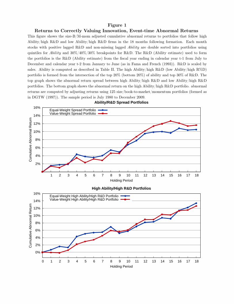
Figure 1Returns to Correctly Valuing Innovation, Event-time Abnormal Returns

This figure shows the size-B/M-mom adjusted cumulative abnormal returns to portfolios that follow highAbility/high R&D and low Ability/high R&D firms in the 18 months following formation. Each monthstocks with positive lagged R&D and non-missing lagged Ability are double sorted into portfolios usingquintiles for Ability and 30%/40%/30% breakpoints for R&D. The R&D (Ability estimate) used to formthe portfolios is the R&D (Ability estimate) from the fiscal year ending in calendar year t-1 from July toDecember and calendar year t-2 from January to June (as in Fama and French (1993)). R&D is scaled bysales. Ability is computed as described in Table II. The high Ability/high R&D (low Ability/high R%D)portfolio is formed from the intersection of the top 20% (bottom 20%) of ability and top 30% of R&D. Thetop graph shows the abnormal return spread between high Ability/high R&D and low Ability/high R&Dportfolios. The bottom graph shows the abnormal return on the high Ability/high R&D portfolio. abnormalreturns are computed by adjusting returns using 125 size/book-to-market/momentum portfolios (formed asin DGTW (1997)). The sample period is July 1980 to December 2009.

2%

4%

6%

8%

10%

12%

14%

16%

1 2 3 4 5 6 7 8 9 10 11 12 13 14 15 16 17 18

Cum

ulat

ive

Abn

orm

al R

etur

n

Holding Period

Ability/R&D Spread Portfolios

Equal-Weight Spread PortfolioValue-Weight Spread Portfolio

0%

2%

4%

6%

8%

10%

12%

14%

16%

0 1 2 3 4 5 6 7 8 9 10 11 12 13 14 15 16 17 18

Cum

ulat

ive

Abn

orm

al R

etur

n

Holding Period

High Ability/High R&D Portfolios

Equal-Weight High Ability/High R&D PortfolioValue-Weight High Ability/High R&D Portfolio

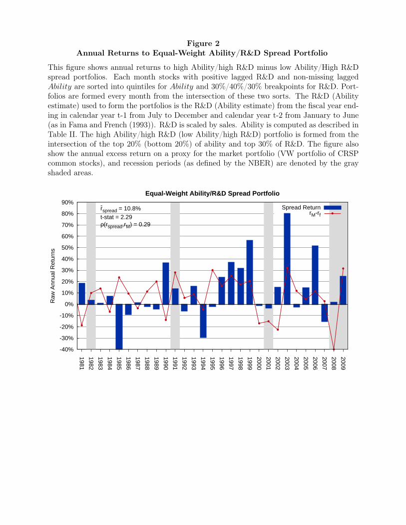
Figure 2Annual Returns to Equal-Weight Ability/R&D Spread Portfolio

This figure shows annual returns to high Ability/high R&D minus low Ability/High R&Dspread portfolios. Each month stocks with positive lagged R&D and non-missing laggedAbility are sorted into quintiles for Ability and 30%/40%/30% breakpoints for R&D. Port-folios are formed every month from the intersection of these two sorts. The R&D (Abilityestimate) used to form the portfolios is the R&D (Ability estimate) from the fiscal year end-ing in calendar year t-1 from July to December and calendar year t-2 from January to June(as in Fama and French (1993)). R&D is scaled by sales. Ability is computed as described inTable II. The high Ability/high R&D (low Ability/high R&D) portfolio is formed from theintersection of the top 20% (bottom 20%) of ability and top 30% of R&D. The figure alsoshow the annual excess return on a proxy for the market portfolio (VW portfolio of CRSPcommon stocks), and recession periods (as defined by the NBER) are denoted by the grayshaded areas.

-40%

-30%

-20%

-10%

0%

10%

20%

30%

40%

50%

60%

70%

80%

90%

1981

1982

1983

1984

1985

1986

1987

1988

1989

1990

1991

1992

1993

1994

1995

1996

1997

1998

1999

2000

2001

2002

2003

2004

2005

2006

2007

2008

2009

Raw

Ann

ual R

etur

ns

Equal-Weight Ability/R&D Spread Portfolio

r-spread = 10.8%

t-stat = 2.29ρ(rspread,rM) = 0.29

Spread ReturnrM-rf

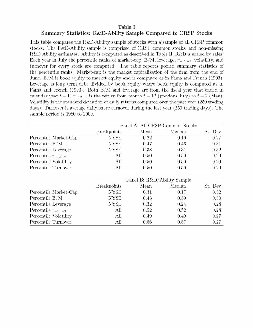
Table ISummary Statistics: R&D-Ability Sample Compared to CRSP Stocks

This table compares the R&D-Ability sample of stocks with a sample of all CRSP commonstocks. The R&D-Ability sample is comprised of CRSP common stocks, and non-missingR&D Ability estimates. Ability is computed as described in Table II. R&D is scaled by sales.Each year in July the percentile ranks of market-cap, B/M, leverage, r−12,−2, volatility, andturnover for every stock are computed. The table reports pooled summary statistics ofthe percentile ranks. Market-cap is the market capitalization of the firm from the end ofJune. B/M is book equity to market equity and is computed as in Fama and French (1993).Leverage is long term debt divided by book equity where book equity is computed as inFama and French (1993). Both B/M and leverage are from the fiscal year that ended incalendar year t− 1. r−12,−2 is the return from month t− 12 (previous July) to t− 2 (May).Volatility is the standard deviation of daily returns computed over the past year (250 tradingdays). Turnover is average daily share turnover during the last year (250 trading days). Thesample period is 1980 to 2009.

Panel A: All CRSP Common StocksBreakpoints Mean Median St. Dev

Percentile Market-Cap NYSE 0.22 0.10 0.27Percentile B/M NYSE 0.47 0.46 0.31Percentile Leverage NYSE 0.38 0.31 0.32Percentile r−12,−2 All 0.50 0.50 0.29Percentile Volatility All 0.50 0.50 0.29Percentile Turnover All 0.50 0.50 0.29

Panel B: R&D/Ability SampleBreakpoints Mean Median St. Dev

Percentile Market-Cap NYSE 0.31 0.17 0.32Percentile B/M NYSE 0.43 0.39 0.30Percentile Leverage NYSE 0.32 0.24 0.28Percentile r−12,−2 All 0.52 0.52 0.28Percentile Volatility All 0.49 0.49 0.27Percentile Turnover All 0.56 0.57 0.27

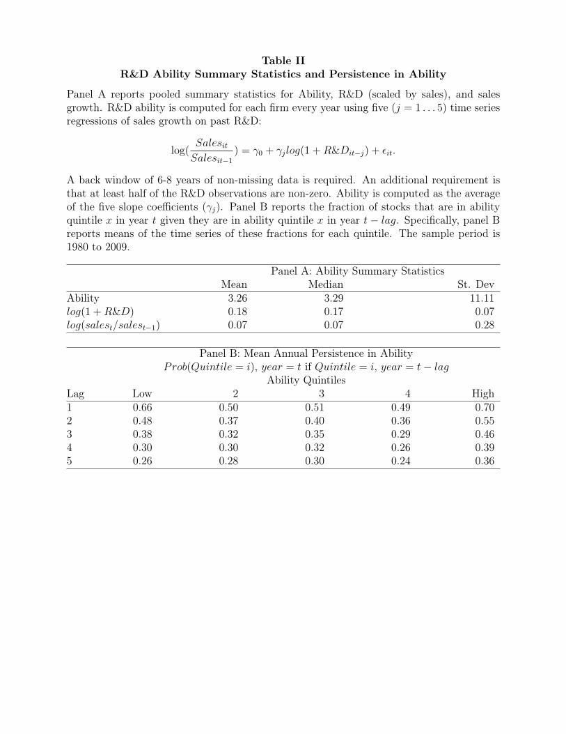
Table IIR&D Ability Summary Statistics and Persistence in Ability

Panel A reports pooled summary statistics for Ability, R&D (scaled by sales), and salesgrowth. R&D ability is computed for each firm every year using five (j = 1 . . . 5) time seriesregressions of sales growth on past R&D:

log(SalesitSalesit−1

) = γ0 + γjlog(1 +R&Dit−j) + εit.

A back window of 6-8 years of non-missing data is required. An additional requirement isthat at least half of the R&D observations are non-zero. Ability is computed as the averageof the five slope coefficients (γj). Panel B reports the fraction of stocks that are in abilityquintile x in year t given they are in ability quintile x in year t− lag. Specifically, panel Breports means of the time series of these fractions for each quintile. The sample period is1980 to 2009.

Panel A: Ability Summary StatisticsMean Median St. Dev

Ability 3.26 3.29 11.11log(1 +R&D) 0.18 0.17 0.07log(salest/salest−1) 0.07 0.07 0.28

Panel B: Mean Annual Persistence in AbilityProb(Quintile = i), year = t if Quintile = i, year = t− lag

Ability QuintilesLag Low 2 3 4 High1 0.66 0.50 0.51 0.49 0.702 0.48 0.37 0.40 0.36 0.553 0.38 0.32 0.35 0.29 0.464 0.30 0.30 0.32 0.26 0.395 0.26 0.28 0.30 0.24 0.36

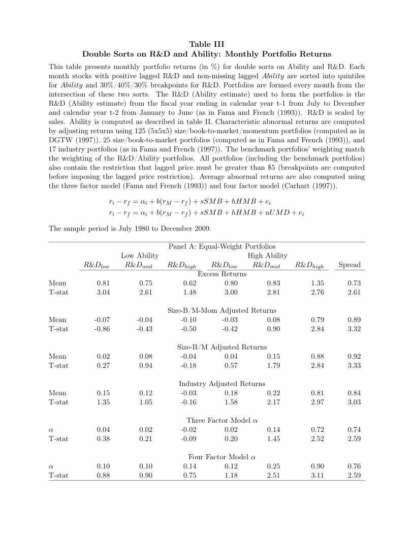
Table IIIDouble Sorts on R&D and Ability: Monthly Portfolio Returns

This table presents monthly portfolio returns (in %) for double sorts on Ability and R&D. Eachmonth stocks with positive lagged R&D and non-missing lagged Ability are sorted into quintilesfor Ability and 30%/40%/30% breakpoints for R&D. Portfolios are formed every month from theintersection of these two sorts. The R&D (Ability estimate) used to form the portfolios is theR&D (Ability estimate) from the fiscal year ending in calendar year t-1 from July to Decemberand calendar year t-2 from January to June (as in Fama and French (1993)). R&D is scaled bysales. Ability is computed as described in table II. Characteristic abnormal returns are computedby adjusting returns using 125 (5x5x5) size/book-to-market/momentum portfolios (computed as inDGTW (1997)), 25 size/book-to-market portfolios (computed as in Fama and French (1993)), and17 industry portfolios (as in Fama and French (1997)). The benchmark portfolios’ weighting matchthe weighting of the R&D/Ability portfolios. All portfolios (including the benchmark portfolios)also contain the restriction that lagged price must be greater than $5 (breakpoints are computedbefore imposing the lagged price restriction). Average abnormal returns are also computed usingthe three factor model (Fama and French (1993)) and four factor model (Carhart (1997)).

ri − rf = αi + b(rM − rf ) + sSMB + hHMB + ei

ri − rf = αi + b(rM − rf ) + sSMB + hHMB + uUMD + ei

The sample period is July 1980 to December 2009.

Panel A: Equal-Weight PortfoliosLow Ability High Ability

R&Dlow R&Dmid R&Dhigh R&Dlow R&Dmid R&Dhigh SpreadExcess Returns

Mean 0.81 0.75 0.62 0.80 0.83 1.35 0.73T-stat 3.04 2.61 1.48 3.00 2.81 2.76 2.61

Size-B/M-Mom Adjusted ReturnsMean -0.07 -0.04 -0.10 -0.03 0.08 0.79 0.89T-stat -0.86 -0.43 -0.50 -0.42 0.90 2.84 3.32

Size-B/M Adjusted ReturnsMean 0.02 0.08 -0.04 0.04 0.15 0.88 0.92T-stat 0.27 0.94 -0.18 0.57 1.79 2.84 3.33

Industry Adjusted ReturnsMean 0.15 0.12 -0.03 0.18 0.22 0.81 0.84T-stat 1.35 1.05 -0.16 1.58 2.17 2.97 3.03

Three Factor Model αα 0.04 0.02 -0.02 0.02 0.14 0.72 0.74T-stat 0.38 0.21 -0.09 0.20 1.45 2.52 2.59

Four Factor Model αα 0.10 0.10 0.14 0.12 0.25 0.90 0.76T-stat 0.88 0.90 0.75 1.18 2.51 3.11 2.59

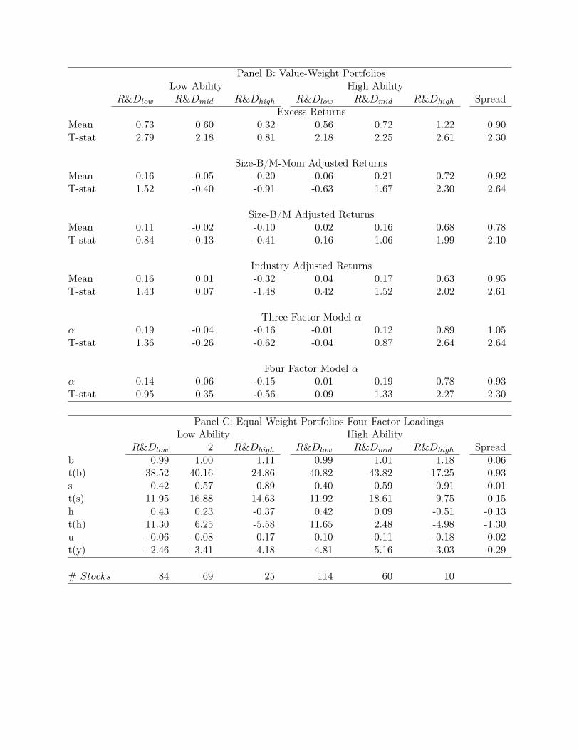
Panel B: Value-Weight PortfoliosLow Ability High Ability


Mean 0.73 0.60 0.32 0.56 0.72 1.22 0.90T-stat 2.79 2.18 0.81 2.18 2.25 2.61 2.30

Size-B/M-Mom Adjusted ReturnsMean 0.16 -0.05 -0.20 -0.06 0.21 0.72 0.92T-stat 1.52 -0.40 -0.91 -0.63 1.67 2.30 2.64

Size-B/M Adjusted ReturnsMean 0.11 -0.02 -0.10 0.02 0.16 0.68 0.78T-stat 0.84 -0.13 -0.41 0.16 1.06 1.99 2.10

Industry Adjusted ReturnsMean 0.16 0.01 -0.32 0.04 0.17 0.63 0.95T-stat 1.43 0.07 -1.48 0.42 1.52 2.02 2.61

Three Factor Model αα 0.19 -0.04 -0.16 -0.01 0.12 0.89 1.05T-stat 1.36 -0.26 -0.62 -0.04 0.87 2.64 2.64

Four Factor Model αα 0.14 0.06 -0.15 0.01 0.19 0.78 0.93T-stat 0.95 0.35 -0.56 0.09 1.33 2.27 2.30

Panel C: Equal Weight Portfolios Four Factor LoadingsLow Ability High Ability

R&Dlow 2 R&Dhigh R&Dlow R&Dmid R&Dhigh Spreadb 0.99 1.00 1.11 0.99 1.01 1.18 0.06t(b) 38.52 40.16 24.86 40.82 43.82 17.25 0.93s 0.42 0.57 0.89 0.40 0.59 0.91 0.01t(s) 11.95 16.88 14.63 11.92 18.61 9.75 0.15h 0.43 0.23 -0.37 0.42 0.09 -0.51 -0.13t(h) 11.30 6.25 -5.58 11.65 2.48 -4.98 -1.30u -0.06 -0.08 -0.17 -0.10 -0.11 -0.18 -0.02t(y) -2.46 -3.41 -4.18 -4.81 -5.16 -3.03 -0.29

# Stocks 84 69 25 114 60 10

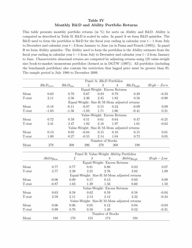
Table IVMonthly R&D and Ability Portfolio Returns

This table presents monthly portfolio returns (in %) for sorts on Ability and R&D. Ability iscomputed as described in Table II. R&D is scaled by sales. In panel A we form R&D quintiles. TheR&D used to form the portfolios is R&D for the fiscal year ending in calendar year t− 1 from Julyto December and calendar year t−2 from January to June (as in Fama and French (1993)). In panelB we form Ability quintiles. The Ability used to form the portfolios is the Ability estimate from thefiscal year ending in calendar year t−1 from July to December and calendar year t−2 from Januaryto June. Characteristic abnormal returns are computed by adjusting returns using 125 value-weightsize/book-to-market/momentum portfolios (formed as in DGTW (1997)). All portfolios (includingthe benchmark portfolios) also contain the restriction that lagged price must be greater than $5.The sample period is July 1980 to December 2009.

Panel A: R&D PortfoliosR&Dzero R&Dlow 2 3 4 R&Dhigh High− Zero

Equal-Weight: Excess ReturnsMean 0.63 0.70 0.67 0.83 0.79 0.29 -0.33T-stat 2.11 2.56 2.36 2.35 1.82 0.58 -0.90

Equal-Weight: Size-B/M-Mom adjusted returnsMean -0.18 -0.11 -0.07 0.15 0.24 -0.09 0.09T-stat -1.63 -1.56 -1.03 1.71 1.66 -0.41 0.31

Value-Weight: Excess ReturnsMean 0.72 0.59 0.51 0.61 0.64 0.47 -0.25T-stat 2.41 2.47 1.92 2.16 1.97 1.01 -0.62

Value-Weight: Size-B/M-Mom adjusted returnsMean 0.13 0.02 -0.04 0.15 0.10 0.15 0.01T-stat 1.00 0.27 -0.55 2.14 1.04 0.72 0.05

Number of StocksMean 278 308 296 278 268 198

Panel B: Value-Weight Ability PortfoliosAbilitylow 2 3 4 Abilityhigh High− Low

Equal-Weight: Excess ReturnsMean 0.77 0.77 0.81 0.86 0.83 0.07T-stat 2.77 2.39 2.25 2.76 3.02 1.09

Equal-Weight: Size-B/M-Mom adjusted returnsMean -0.06 0.09 0.17 0.13 0.03 0.09T-stat -0.87 1.03 1.39 1.56 0.60 1.50

Value-Weight: Excess ReturnsMean 0.63 0.58 0.62 0.59 0.58 -0.04T-stat 2.59 2.11 2.13 2.12 2.22 -0.34

Value-Weight: Size-B/M-Mom adjusted returnsMean 0.06 0.06 0.05 0.12 0.04 -0.03T-stat 0.99 0.70 0.50 1.49 0.52 -0.31

Number of StocksMean 188 170 155 174 194

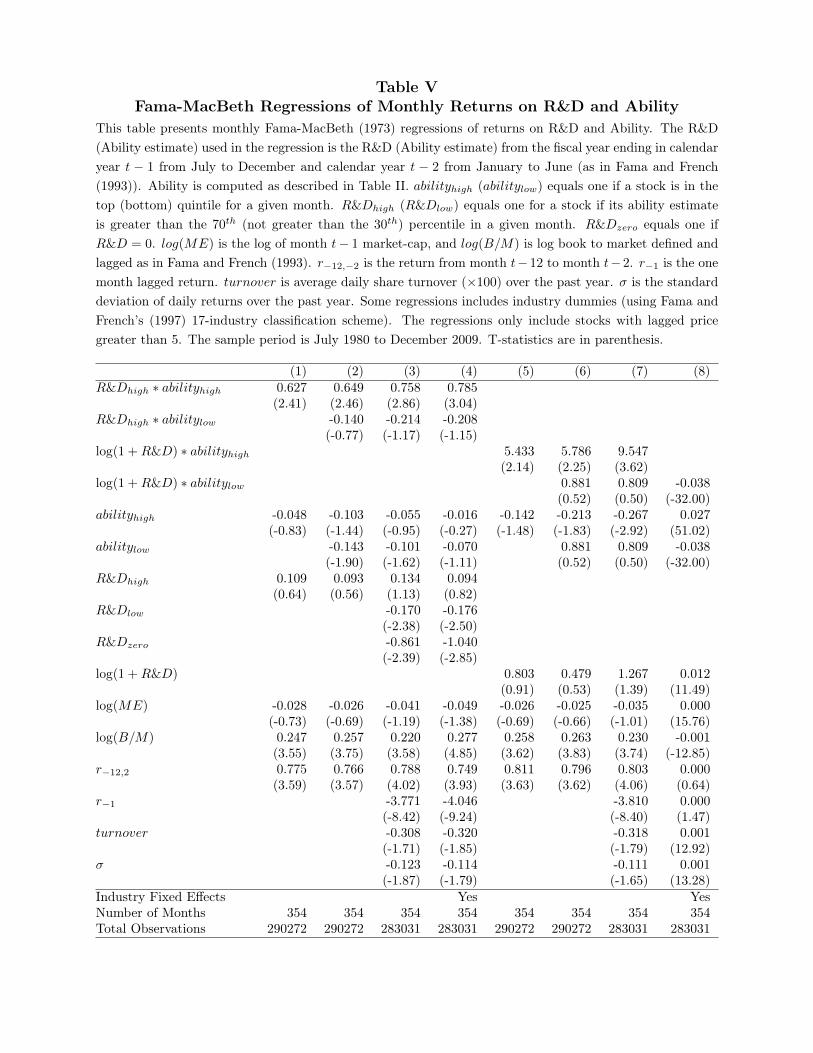
Table VFama-MacBeth Regressions of Monthly Returns on R&D and Ability

This table presents monthly Fama-MacBeth (1973) regressions of returns on R&D and Ability. The R&D(Ability estimate) used in the regression is the R&D (Ability estimate) from the fiscal year ending in calendaryear t − 1 from July to December and calendar year t − 2 from January to June (as in Fama and French(1993)). Ability is computed as described in Table II. abilityhigh (abilitylow) equals one if a stock is in thetop (bottom) quintile for a given month. R&Dhigh (R&Dlow) equals one for a stock if its ability estimateis greater than the 70th (not greater than the 30th) percentile in a given month. R&Dzero equals one ifR&D = 0. log(ME) is the log of month t− 1 market-cap, and log(B/M) is log book to market defined andlagged as in Fama and French (1993). r−12,−2 is the return from month t− 12 to month t− 2. r−1 is the onemonth lagged return. turnover is average daily share turnover (×100) over the past year. σ is the standarddeviation of daily returns over the past year. Some regressions includes industry dummies (using Fama andFrench’s (1997) 17-industry classification scheme). The regressions only include stocks with lagged pricegreater than 5. The sample period is July 1980 to December 2009. T-statistics are in parenthesis.

(1) (2) (3) (4) (5) (6) (7) (8)R&Dhigh ∗ abilityhigh 0.627 0.649 0.758 0.785

(2.41) (2.46) (2.86) (3.04)R&Dhigh ∗ abilitylow -0.140 -0.214 -0.208

(-0.77) (-1.17) (-1.15)log(1 +R&D) ∗ abilityhigh 5.433 5.786 9.547

(2.14) (2.25) (3.62)log(1 +R&D) ∗ abilitylow 0.881 0.809 -0.038

(0.52) (0.50) (-32.00)abilityhigh -0.048 -0.103 -0.055 -0.016 -0.142 -0.213 -0.267 0.027

(-0.83) (-1.44) (-0.95) (-0.27) (-1.48) (-1.83) (-2.92) (51.02)abilitylow -0.143 -0.101 -0.070 0.881 0.809 -0.038

(-1.90) (-1.62) (-1.11) (0.52) (0.50) (-32.00)R&Dhigh 0.109 0.093 0.134 0.094

(0.64) (0.56) (1.13) (0.82)R&Dlow -0.170 -0.176

(-2.38) (-2.50)R&Dzero -0.861 -1.040

(-2.39) (-2.85)log(1 +R&D) 0.803 0.479 1.267 0.012

(0.91) (0.53) (1.39) (11.49)log(ME) -0.028 -0.026 -0.041 -0.049 -0.026 -0.025 -0.035 0.000

(-0.73) (-0.69) (-1.19) (-1.38) (-0.69) (-0.66) (-1.01) (15.76)log(B/M) 0.247 0.257 0.220 0.277 0.258 0.263 0.230 -0.001

(3.55) (3.75) (3.58) (4.85) (3.62) (3.83) (3.74) (-12.85)r−12,2 0.775 0.766 0.788 0.749 0.811 0.796 0.803 0.000

(3.59) (3.57) (4.02) (3.93) (3.63) (3.62) (4.06) (0.64)r−1 -3.771 -4.046 -3.810 0.000

(-8.42) (-9.24) (-8.40) (1.47)turnover -0.308 -0.320 -0.318 0.001

(-1.71) (-1.85) (-1.79) (12.92)σ -0.123 -0.114 -0.111 0.001

(-1.87) (-1.79) (-1.65) (13.28)Industry Fixed Effects Yes YesNumber of Months 354 354 354 354 354 354 354 354Total Observations 290272 290272 283031 283031 290272 290272 283031 283031

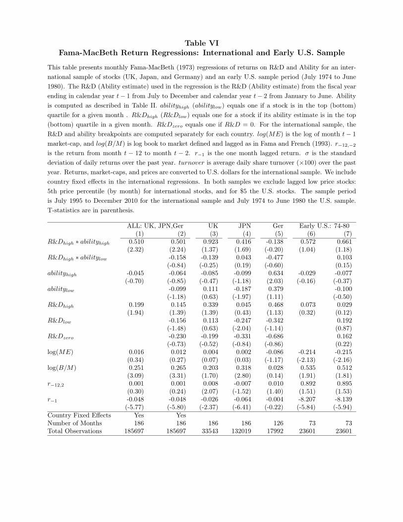
Table VIFama-MacBeth Return Regressions: International and Early U.S. Sample

This table presents monthly Fama-MacBeth (1973) regressions of returns on R&D and Ability for an inter-national sample of stocks (UK, Japan, and Germany) and an early U.S. sample period (July 1974 to June1980). The R&D (Ability estimate) used in the regression is the R&D (Ability estimate) from the fiscal yearending in calendar year t− 1 from July to December and calendar year t− 2 from January to June. Abilityis computed as described in Table II. abilityhigh (abilitylow) equals one if a stock is in the top (bottom)quartile for a given month . R&Dhigh (R&Dlow) equals one for a stock if its ability estimate is in the top(bottom) quartile in a given month. R&Dzero equals one if R&D = 0. For the international sample, theR&D and ability breakpoints are computed separately for each country. log(ME) is the log of month t− 1

market-cap, and log(B/M) is log book to market defined and lagged as in Fama and French (1993). r−12,−2

is the return from month t − 12 to month t − 2. r−1 is the one month lagged return. σ is the standarddeviation of daily returns over the past year. turnover is average daily share turnover (×100) over the pastyear. Returns, market-caps, and prices are converted to U.S. dollars for the international sample. We includecountry fixed effects in the international regressions. In both samples we exclude lagged low price stocks:5th price percentile (by month) for international stocks, and for $5 the U.S. stocks. The sample periodis July 1995 to December 2010 for the international sample and July 1974 to June 1980 the U.S. sample.T-statistics are in parenthesis.

ALL: UK, JPN,Ger UK JPN Ger Early U.S.: 74-80(1) (2) (3) (4) (5) (6) (7)

R&Dhigh ∗ abilityhigh 0.510 0.501 0.923 0.416 -0.138 0.572 0.661(2.32) (2.24) (1.37) (1.69) (-0.20) (1.04) (1.18)

R&Dhigh ∗ abilitylow -0.158 -0.139 0.043 -0.477 0.103(-0.84) (-0.25) (0.19) (-0.60) (0.15)

abilityhigh -0.045 -0.064 -0.085 -0.099 0.634 -0.029 -0.077(-0.70) (-0.85) (-0.47) (-1.18) (2.03) (-0.16) (-0.37)

abilitylow -0.099 0.111 -0.187 0.379 -0.100(-1.18) (0.63) (-1.97) (1.11) (-0.50)

R&Dhigh 0.199 0.145 0.339 0.045 0.468 0.073 0.029(1.94) (1.39) (1.39) (0.43) (1.13) (0.32) (0.12)

R&Dlow -0.156 0.113 -0.247 -0.342 0.192(-1.48) (0.63) (-2.04) (-1.14) (0.87)

R&Dzero -0.230 -0.199 -0.331 -0.686 0.162(-0.73) (-0.52) (-0.84) (-0.86) (0.22)

log(ME) 0.016 0.012 0.004 0.002 -0.086 -0.214 -0.215(0.34) (0.27) (0.07) (0.03) (-1.17) (-2.13) (-2.16)

log(B/M) 0.251 0.265 0.203 0.318 0.028 0.535 0.512(3.09) (3.31) (1.70) (2.80) (0.14) (1.91) (1.81)

r−12,2 0.001 0.001 0.008 -0.007 0.010 0.892 0.895(0.30) (0.24) (2.07) (-1.52) (1.40) (1.51) (1.53)

r−1 -0.048 -0.048 -0.026 -0.064 -0.004 -8.207 -8.139(-5.77) (-5.80) (-2.37) (-6.41) (-0.22) (-5.84) (-5.94)

Country Fixed Effects Yes YesNumber of Months 186 186 186 186 126 73 73Total Observations 185697 185697 33543 132019 17992 23601 23601

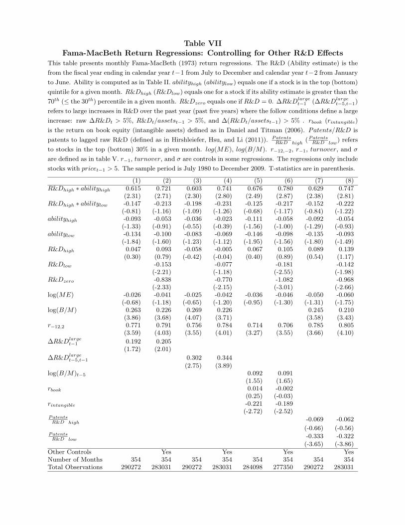
Table VIIFama-MacBeth Return Regressions: Controlling for Other R&D Effects

This table presents monthly Fama-MacBeth (1973) return regressions. The R&D (Ability estimate) is thefrom the fiscal year ending in calendar year t−1 from July to December and calendar year t−2 from Januaryto June. Ability is computed as in Table II. abilityhigh (abilitylow) equals one if a stock is in the top (bottom)quintile for a given month. R&Dhigh (R&Dlow) equals one for a stock if its ability estimate is greater than the70th (≤ the 30th) percentile in a given month. R&Dzero equals one if R&D = 0. ∆R&Dlarge

t−1 (∆R&Dlarget−5,t−1)

refers to large increases in R&D over the past year (past five years) where the follow conditions define a largeincrease: raw ∆R&Dt > 5%, R&Dt/assetst−1 > 5%, and ∆(R&Dt/assetst−1) > 5% . rbook (rintangible)is the return on book equity (intangible assets) defined as in Daniel and Titman (2006). Patents/R&D ispatents to lagged raw R&D (defined as in Hirshleiefer, Hsu, and Li (2011)). Patents

R&D high(Patents

R&D low) refers

to stocks in the top (bottom) 30% in a given month. log(ME), log(B/M). r−12,−2, r−1, turnover, and σare defined as in table V. r−1, turnover, and σ are controls in some regressions. The regressions only includestocks with pricet−1 > 5. The sample period is July 1980 to December 2009. T-statistics are in parenthesis.

(1) (2) (3) (4) (5) (6) (7) (8)R&Dhigh ∗ abilityhigh 0.615 0.721 0.603 0.741 0.676 0.780 0.629 0.747

(2.31) (2.71) (2.30) (2.80) (2.49) (2.87) (2.38) (2.81)R&Dhigh ∗ abilitylow -0.147 -0.213 -0.198 -0.231 -0.125 -0.217 -0.152 -0.222

(-0.81) (-1.16) (-1.09) (-1.26) (-0.68) (-1.17) (-0.84) (-1.22)abilityhigh -0.093 -0.053 -0.036 -0.023 -0.111 -0.058 -0.092 -0.054

(-1.33) (-0.91) (-0.55) (-0.39) (-1.56) (-1.00) (-1.29) (-0.93)abilitylow -0.134 -0.100 -0.083 -0.069 -0.146 -0.098 -0.135 -0.093

(-1.84) (-1.60) (-1.23) (-1.12) (-1.95) (-1.56) (-1.80) (-1.49)R&Dhigh 0.047 0.093 -0.058 -0.005 0.067 0.105 0.089 0.139

(0.30) (0.79) (-0.42) (-0.04) (0.40) (0.89) (0.54) (1.17)R&Dlow -0.153 -0.077 -0.181 -0.142

(-2.21) (-1.18) (-2.55) (-1.98)R&Dzero -0.838 -0.770 -1.082 -0.968

(-2.33) (-2.15) (-3.01) (-2.66)log(ME) -0.026 -0.041 -0.025 -0.042 -0.036 -0.046 -0.050 -0.060

(-0.68) (-1.18) (-0.65) (-1.20) (-0.95) (-1.30) (-1.31) (-1.75)log(B/M) 0.263 0.226 0.269 0.226 0.245 0.210

(3.86) (3.68) (4.07) (3.71) (3.58) (3.43)r−12,2 0.771 0.791 0.756 0.784 0.714 0.706 0.785 0.805

(3.59) (4.03) (3.55) (4.01) (3.27) (3.55) (3.66) (4.10)∆R&Dlarge

t−1 0.192 0.205(1.72) (2.01)

∆R&Dlarget−5,t−1 0.302 0.344

(2.75) (3.89)log(B/M)t−5 0.092 0.091

(1.55) (1.65)rbook 0.014 -0.002

(0.25) (-0.03)rintangible -0.221 -0.189

(-2.72) (-2.52)PatentsR&D high

-0.069 -0.062(-0.66) (-0.56)

PatentsR&D low

-0.333 -0.322(-3.65) (-3.86)

Other Controls Yes Yes Yes YesNumber of Months 354 354 354 354 354 354 354 354Total Observations 290272 283031 290272 283031 284098 277350 290272 283031

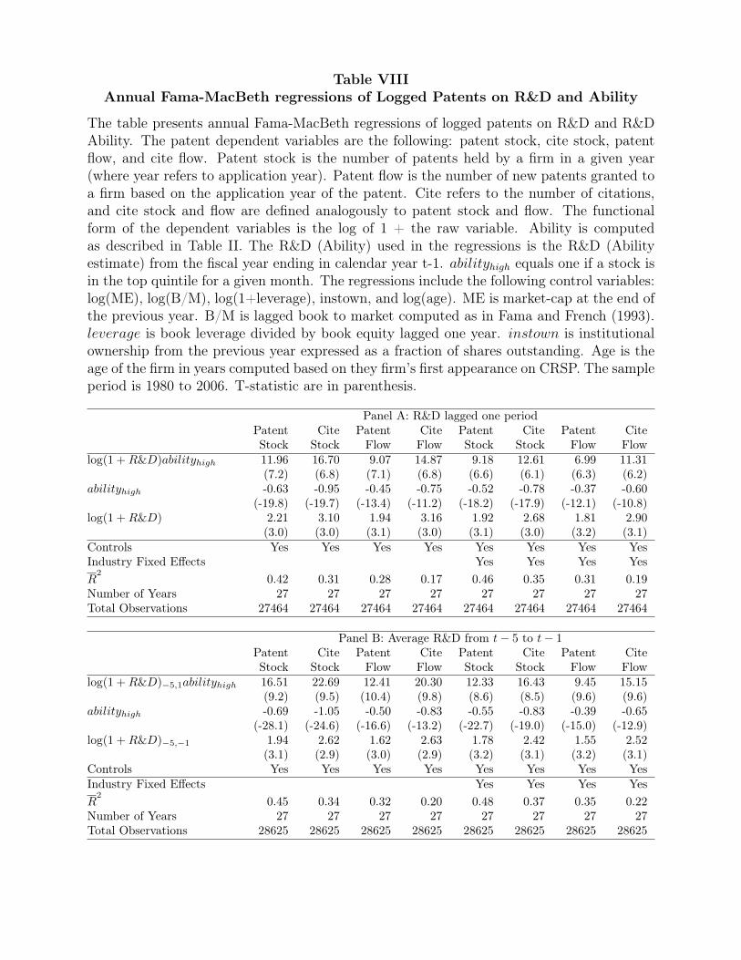
Table VIIIAnnual Fama-MacBeth regressions of Logged Patents on R&D and Ability

The table presents annual Fama-MacBeth regressions of logged patents on R&D and R&DAbility. The patent dependent variables are the following: patent stock, cite stock, patentflow, and cite flow. Patent stock is the number of patents held by a firm in a given year(where year refers to application year). Patent flow is the number of new patents granted toa firm based on the application year of the patent. Cite refers to the number of citations,and cite stock and flow are defined analogously to patent stock and flow. The functionalform of the dependent variables is the log of 1 + the raw variable. Ability is computedas described in Table II. The R&D (Ability) used in the regressions is the R&D (Abilityestimate) from the fiscal year ending in calendar year t-1. abilityhigh equals one if a stock isin the top quintile for a given month. The regressions include the following control variables:log(ME), log(B/M), log(1+leverage), instown, and log(age). ME is market-cap at the end ofthe previous year. B/M is lagged book to market computed as in Fama and French (1993).leverage is book leverage divided by book equity lagged one year. instown is institutionalownership from the previous year expressed as a fraction of shares outstanding. Age is theage of the firm in years computed based on they firm’s first appearance on CRSP. The sampleperiod is 1980 to 2006. T-statistic are in parenthesis.

Panel A: R&D lagged one periodPatent Cite Patent Cite Patent Cite Patent CiteStock Stock Flow Flow Stock Stock Flow Flow

log(1 +R&D)abilityhigh 11.96 16.70 9.07 14.87 9.18 12.61 6.99 11.31(7.2) (6.8) (7.1) (6.8) (6.6) (6.1) (6.3) (6.2)

abilityhigh -0.63 -0.95 -0.45 -0.75 -0.52 -0.78 -0.37 -0.60(-19.8) (-19.7) (-13.4) (-11.2) (-18.2) (-17.9) (-12.1) (-10.8)

log(1 +R&D) 2.21 3.10 1.94 3.16 1.92 2.68 1.81 2.90(3.0) (3.0) (3.1) (3.0) (3.1) (3.0) (3.2) (3.1)

Controls Yes Yes Yes Yes Yes Yes Yes YesIndustry Fixed Effects Yes Yes Yes YesR

20.42 0.31 0.28 0.17 0.46 0.35 0.31 0.19

Number of Years 27 27 27 27 27 27 27 27Total Observations 27464 27464 27464 27464 27464 27464 27464 27464

Panel B: Average R&D from t− 5 to t− 1Patent Cite Patent Cite Patent Cite Patent CiteStock Stock Flow Flow Stock Stock Flow Flow

log(1 +R&D)−5,1abilityhigh 16.51 22.69 12.41 20.30 12.33 16.43 9.45 15.15(9.2) (9.5) (10.4) (9.8) (8.6) (8.5) (9.6) (9.6)

abilityhigh -0.69 -1.05 -0.50 -0.83 -0.55 -0.83 -0.39 -0.65(-28.1) (-24.6) (-16.6) (-13.2) (-22.7) (-19.0) (-15.0) (-12.9)

log(1 +R&D)−5,−1 1.94 2.62 1.62 2.63 1.78 2.42 1.55 2.52(3.1) (2.9) (3.0) (2.9) (3.2) (3.1) (3.2) (3.1)

Controls Yes Yes Yes Yes Yes Yes Yes YesIndustry Fixed Effects Yes Yes Yes YesR

20.45 0.34 0.32 0.20 0.48 0.37 0.35 0.22

Number of Years 27 27 27 27 27 27 27 27Total Observations 28625 28625 28625 28625 28625 28625 28625 28625

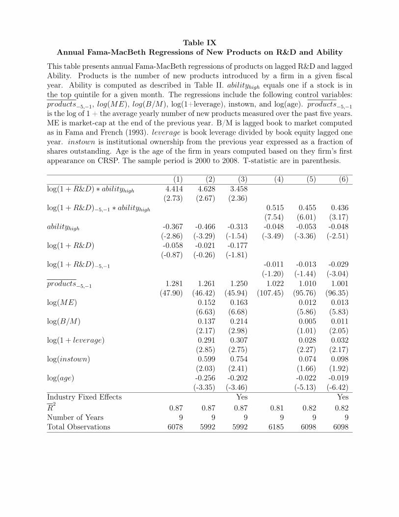
Table IXAnnual Fama-MacBeth Regressions of New Products on R&D and Ability

This table presents annual Fama-MacBeth regressions of products on lagged R&D and laggedAbility. Products is the number of new products introduced by a firm in a given fiscalyear. Ability is computed as described in Table II. abilityhigh equals one if a stock is inthe top quintile for a given month. The regressions include the following control variables:products−5,−1, log(ME), log(B/M), log(1+leverage), instown, and log(age). products−5,−1

is the log of 1 + the average yearly number of new products measured over the past five years.ME is market-cap at the end of the previous year. B/M is lagged book to market computedas in Fama and French (1993). leverage is book leverage divided by book equity lagged oneyear. instown is institutional ownership from the previous year expressed as a fraction ofshares outstanding. Age is the age of the firm in years computed based on they firm’s firstappearance on CRSP. The sample period is 2000 to 2008. T-statistic are in parenthesis.

(1) (2) (3) (4) (5) (6)log(1 +R&D) ∗ abilityhigh 4.414 4.628 3.458

(2.73) (2.67) (2.36)log(1 +R&D)−5,−1 ∗ abilityhigh 0.515 0.455 0.436

(7.54) (6.01) (3.17)abilityhigh -0.367 -0.466 -0.313 -0.048 -0.053 -0.048

(-2.86) (-3.29) (-1.54) (-3.49) (-3.36) (-2.51)log(1 +R&D) -0.058 -0.021 -0.177

(-0.87) (-0.26) (-1.81)log(1 +R&D)−5,−1 -0.011 -0.013 -0.029

(-1.20) (-1.44) (-3.04)products−5,−1 1.281 1.261 1.250 1.022 1.010 1.001

(47.90) (46.42) (45.94) (107.45) (95.76) (96.35)log(ME) 0.152 0.163 0.012 0.013

(6.63) (6.68) (5.86) (5.83)log(B/M) 0.137 0.214 0.005 0.011

(2.17) (2.98) (1.01) (2.05)log(1 + leverage) 0.291 0.307 0.028 0.032

(2.85) (2.75) (2.27) (2.17)log(instown) 0.599 0.754 0.074 0.098

(2.03) (2.41) (1.66) (1.92)log(age) -0.256 -0.202 -0.022 -0.019

(-3.35) (-3.46) (-5.13) (-6.42)Industry Fixed Effects Yes YesR

2 0.87 0.87 0.87 0.81 0.82 0.82Number of Years 9 9 9 9 9 9Total Observations 6078 5992 5992 6185 6098 6098

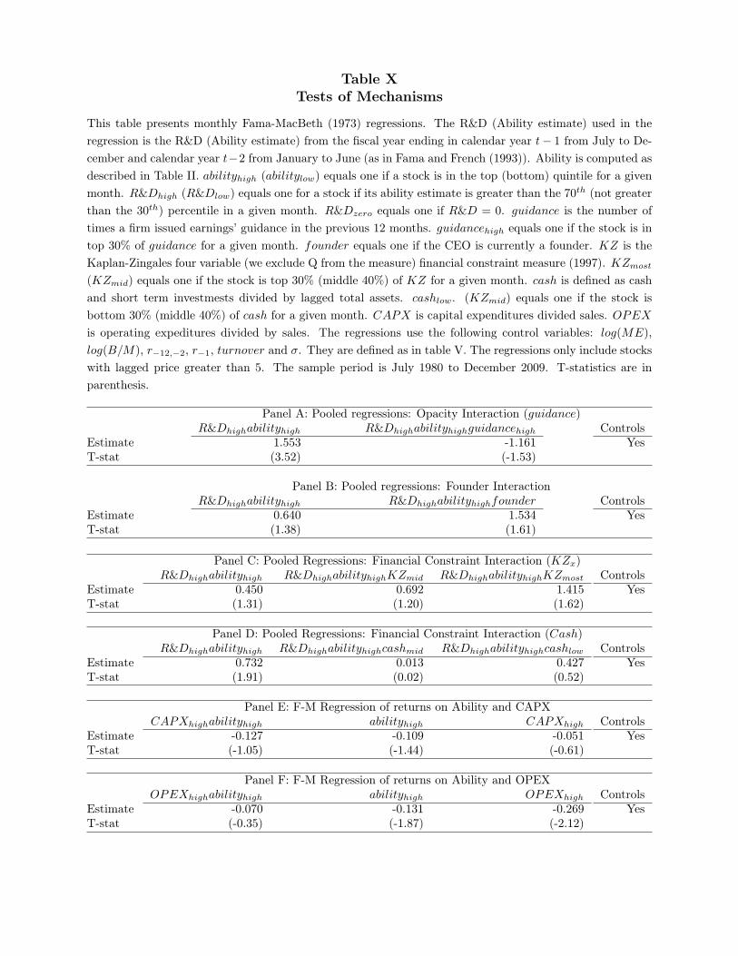
Table XTests of Mechanisms

This table presents monthly Fama-MacBeth (1973) regressions. The R&D (Ability estimate) used in theregression is the R&D (Ability estimate) from the fiscal year ending in calendar year t− 1 from July to De-cember and calendar year t−2 from January to June (as in Fama and French (1993)). Ability is computed asdescribed in Table II. abilityhigh (abilitylow) equals one if a stock is in the top (bottom) quintile for a givenmonth. R&Dhigh (R&Dlow) equals one for a stock if its ability estimate is greater than the 70th (not greaterthan the 30th) percentile in a given month. R&Dzero equals one if R&D = 0. guidance is the number oftimes a firm issued earnings’ guidance in the previous 12 months. guidancehigh equals one if the stock is intop 30% of guidance for a given month. founder equals one if the CEO is currently a founder. KZ is theKaplan-Zingales four variable (we exclude Q from the measure) financial constraint measure (1997). KZmost

(KZmid) equals one if the stock is top 30% (middle 40%) of KZ for a given month. cash is defined as cashand short term investmests divided by lagged total assets. cashlow. (KZmid) equals one if the stock isbottom 30% (middle 40%) of cash for a given month. CAPX is capital expenditures divided sales. OPEXis operating expeditures divided by sales. The regressions use the following control variables: log(ME),log(B/M), r−12,−2, r−1, turnover and σ. They are defined as in table V. The regressions only include stockswith lagged price greater than 5. The sample period is July 1980 to December 2009. T-statistics are inparenthesis.

Panel A: Pooled regressions: Opacity Interaction (guidance)R&Dhighabilityhigh R&Dhighabilityhighguidancehigh Controls

Estimate 1.553 -1.161 YesT-stat (3.52) (-1.53)

Panel B: Pooled regressions: Founder InteractionR&Dhighabilityhigh R&Dhighabilityhighfounder Controls

Estimate 0.640 1.534 YesT-stat (1.38) (1.61)

Panel C: Pooled Regressions: Financial Constraint Interaction (KZx)R&Dhighabilityhigh R&DhighabilityhighKZmid R&DhighabilityhighKZmost Controls

Estimate 0.450 0.692 1.415 YesT-stat (1.31) (1.20) (1.62)

Panel D: Pooled Regressions: Financial Constraint Interaction (Cash)R&Dhighabilityhigh R&Dhighabilityhighcashmid R&Dhighabilityhighcashlow Controls

Estimate 0.732 0.013 0.427 YesT-stat (1.91) (0.02) (0.52)

Panel E: F-M Regression of returns on Ability and CAPXCAPXhighabilityhigh abilityhigh CAPXhigh Controls

Estimate -0.127 -0.109 -0.051 YesT-stat (-1.05) (-1.44) (-0.61)

Panel F: F-M Regression of returns on Ability and OPEXOPEXhighabilityhigh abilityhigh OPEXhigh Controls

Estimate -0.070 -0.131 -0.269 YesT-stat (-0.35) (-1.87) (-2.12)

Appendix:Misvaluing Innovation

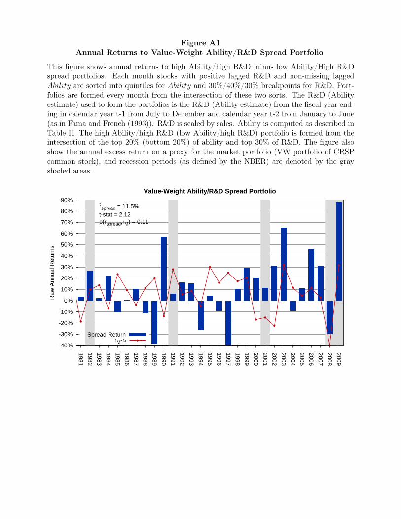
Figure A1Annual Returns to Value-Weight Ability/R&D Spread Portfolio

This figure shows annual returns to high Ability/high R&D minus low Ability/High R&Dspread portfolios. Each month stocks with positive lagged R&D and non-missing laggedAbility are sorted into quintiles for Ability and 30%/40%/30% breakpoints for R&D. Port-folios are formed every month from the intersection of these two sorts. The R&D (Abilityestimate) used to form the portfolios is the R&D (Ability estimate) from the fiscal year end-ing in calendar year t-1 from July to December and calendar year t-2 from January to June(as in Fama and French (1993)). R&D is scaled by sales. Ability is computed as described inTable II. The high Ability/high R&D (low Ability/high R&D) portfolio is formed from theintersection of the top 20% (bottom 20%) of ability and top 30% of R&D. The figure alsoshow the annual excess return on a proxy for the market portfolio (VW portfolio of CRSPcommon stock), and recession periods (as defined by the NBER) are denoted by the grayshaded areas.

-40%

-30%

-20%

-10%

0%

10%

20%

30%

40%

50%

60%

70%

80%

90%

1981

1982

1983

1984

1985

1986

1987

1988

1989

1990

1991

1992

1993

1994

1995

1996

1997

1998

1999

2000

2001

2002

2003

2004

2005

2006

2007

2008

2009

Raw

Ann

ual R

etur

ns

Value-Weight Ability/R&D Spread Portfolio

r-spread = 11.5%

t-stat = 2.12ρ(rspread,rM) = 0.11

Spread ReturnrM-rf

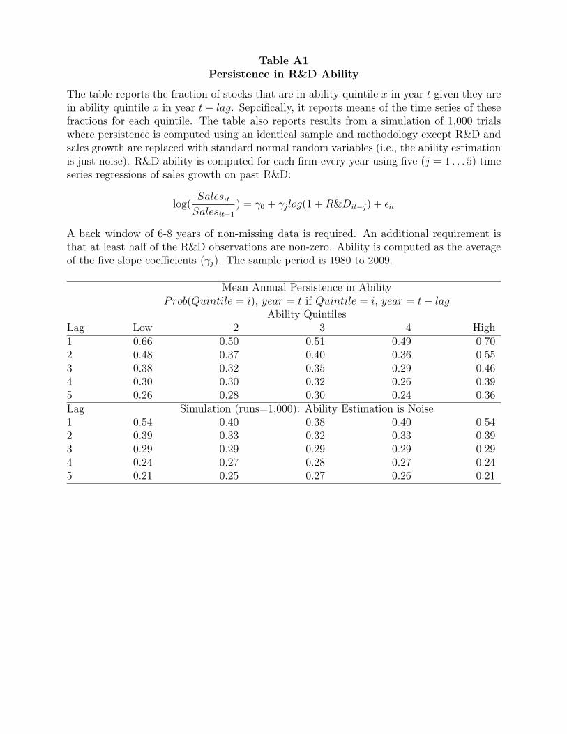
Table A1Persistence in R&D Ability

The table reports the fraction of stocks that are in ability quintile x in year t given they arein ability quintile x in year t− lag. Sepcifically, it reports means of the time series of thesefractions for each quintile. The table also reports results from a simulation of 1,000 trialswhere persistence is computed using an identical sample and methodology except R&D andsales growth are replaced with standard normal random variables (i.e., the ability estimationis just noise). R&D ability is computed for each firm every year using five (j = 1 . . . 5) timeseries regressions of sales growth on past R&D:

log(SalesitSalesit−1

) = γ0 + γjlog(1 +R&Dit−j) + εit

A back window of 6-8 years of non-missing data is required. An additional requirement isthat at least half of the R&D observations are non-zero. Ability is computed as the averageof the five slope coefficients (γj). The sample period is 1980 to 2009.

Mean Annual Persistence in AbilityProb(Quintile = i), year = t if Quintile = i, year = t− lag

Ability QuintilesLag Low 2 3 4 High1 0.66 0.50 0.51 0.49 0.702 0.48 0.37 0.40 0.36 0.553 0.38 0.32 0.35 0.29 0.464 0.30 0.30 0.32 0.26 0.395 0.26 0.28 0.30 0.24 0.36Lag Simulation (runs=1,000): Ability Estimation is Noise1 0.54 0.40 0.38 0.40 0.542 0.39 0.33 0.32 0.33 0.393 0.29 0.29 0.29 0.29 0.294 0.24 0.27 0.28 0.27 0.245 0.21 0.25 0.27 0.26 0.21

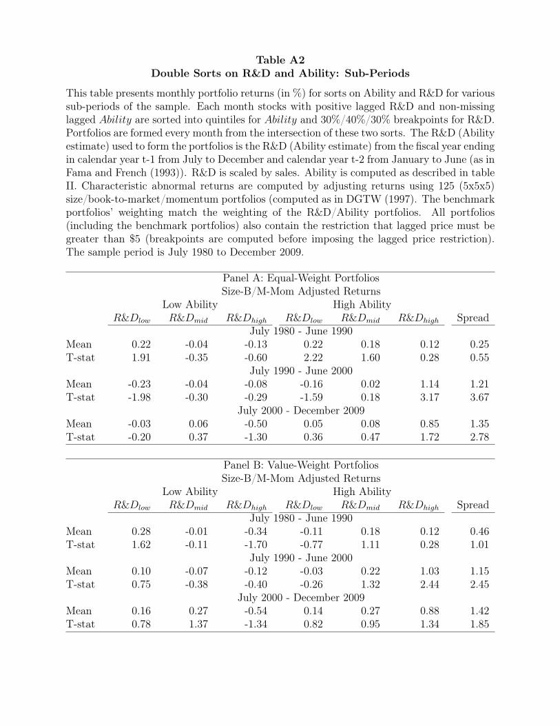
Table A2Double Sorts on R&D and Ability: Sub-Periods

This table presents monthly portfolio returns (in %) for sorts on Ability and R&D for varioussub-periods of the sample. Each month stocks with positive lagged R&D and non-missinglagged Ability are sorted into quintiles for Ability and 30%/40%/30% breakpoints for R&D.Portfolios are formed every month from the intersection of these two sorts. The R&D (Abilityestimate) used to form the portfolios is the R&D (Ability estimate) from the fiscal year endingin calendar year t-1 from July to December and calendar year t-2 from January to June (as inFama and French (1993)). R&D is scaled by sales. Ability is computed as described in tableII. Characteristic abnormal returns are computed by adjusting returns using 125 (5x5x5)size/book-to-market/momentum portfolios (computed as in DGTW (1997). The benchmarkportfolios’ weighting match the weighting of the R&D/Ability portfolios. All portfolios(including the benchmark portfolios) also contain the restriction that lagged price must begreater than $5 (breakpoints are computed before imposing the lagged price restriction).The sample period is July 1980 to December 2009.

Panel A: Equal-Weight PortfoliosSize-B/M-Mom Adjusted Returns

Low Ability High AbilityR&Dlow R&Dmid R&Dhigh R&Dlow R&Dmid R&Dhigh Spread

July 1980 - June 1990Mean 0.22 -0.04 -0.13 0.22 0.18 0.12 0.25T-stat 1.91 -0.35 -0.60 2.22 1.60 0.28 0.55

July 1990 - June 2000Mean -0.23 -0.04 -0.08 -0.16 0.02 1.14 1.21T-stat -1.98 -0.30 -0.29 -1.59 0.18 3.17 3.67

July 2000 - December 2009Mean -0.03 0.06 -0.50 0.05 0.08 0.85 1.35T-stat -0.20 0.37 -1.30 0.36 0.47 1.72 2.78

Panel B: Value-Weight PortfoliosSize-B/M-Mom Adjusted Returns

Low Ability High AbilityR&Dlow R&Dmid R&Dhigh R&Dlow R&Dmid R&Dhigh Spread

July 1980 - June 1990Mean 0.28 -0.01 -0.34 -0.11 0.18 0.12 0.46T-stat 1.62 -0.11 -1.70 -0.77 1.11 0.28 1.01

July 1990 - June 2000Mean 0.10 -0.07 -0.12 -0.03 0.22 1.03 1.15T-stat 0.75 -0.38 -0.40 -0.26 1.32 2.44 2.45

July 2000 - December 2009Mean 0.16 0.27 -0.54 0.14 0.27 0.88 1.42T-stat 0.78 1.37 -1.34 0.82 0.95 1.34 1.85

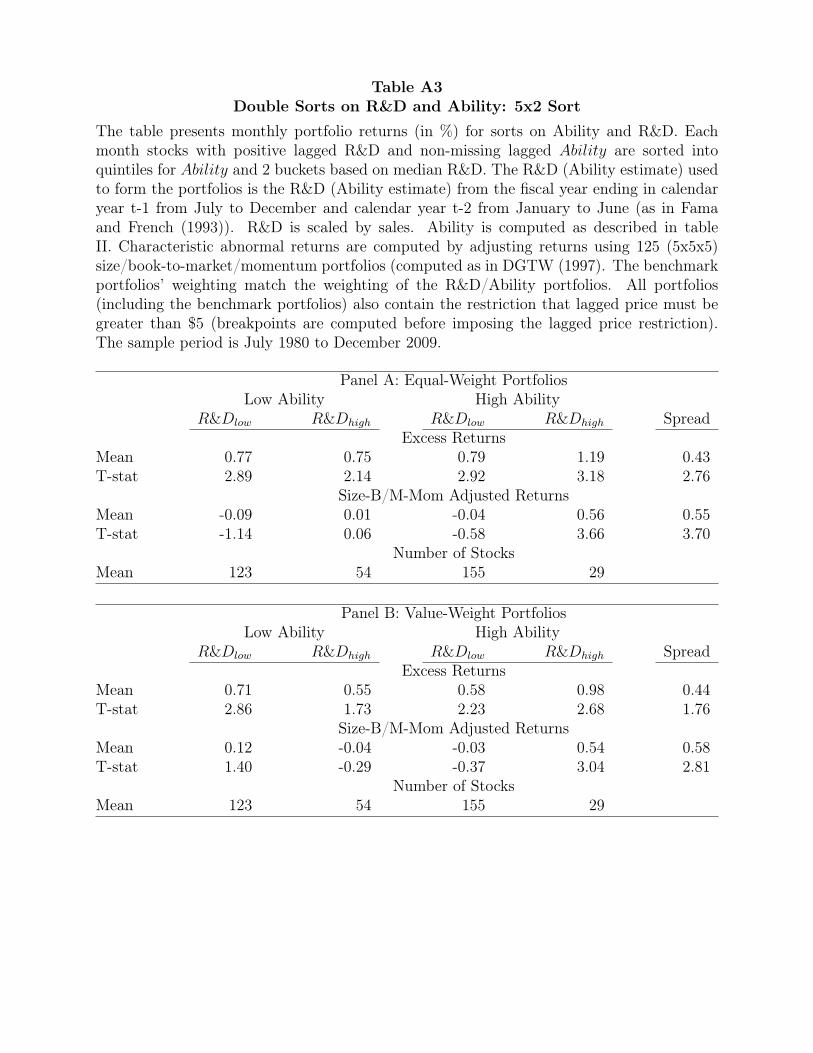
Table A3Double Sorts on R&D and Ability: 5x2 Sort

The table presents monthly portfolio returns (in %) for sorts on Ability and R&D. Eachmonth stocks with positive lagged R&D and non-missing lagged Ability are sorted intoquintiles for Ability and 2 buckets based on median R&D. The R&D (Ability estimate) usedto form the portfolios is the R&D (Ability estimate) from the fiscal year ending in calendaryear t-1 from July to December and calendar year t-2 from January to June (as in Famaand French (1993)). R&D is scaled by sales. Ability is computed as described in tableII. Characteristic abnormal returns are computed by adjusting returns using 125 (5x5x5)size/book-to-market/momentum portfolios (computed as in DGTW (1997). The benchmarkportfolios’ weighting match the weighting of the R&D/Ability portfolios. All portfolios(including the benchmark portfolios) also contain the restriction that lagged price must begreater than $5 (breakpoints are computed before imposing the lagged price restriction).The sample period is July 1980 to December 2009.


R&Dlow R&Dhigh R&Dlow R&Dhigh SpreadExcess Returns

Mean 0.77 0.75 0.79 1.19 0.43T-stat 2.89 2.14 2.92 3.18 2.76

Size-B/M-Mom Adjusted ReturnsMean -0.09 0.01 -0.04 0.56 0.55T-stat -1.14 0.06 -0.58 3.66 3.70

Number of StocksMean 123 54 155 29


R&Dlow R&Dhigh R&Dlow R&Dhigh SpreadExcess Returns

Mean 0.71 0.55 0.58 0.98 0.44T-stat 2.86 1.73 2.23 2.68 1.76

Size-B/M-Mom Adjusted ReturnsMean 0.12 -0.04 -0.03 0.54 0.58T-stat 1.40 -0.29 -0.37 3.04 2.81

Number of StocksMean 123 54 155 29

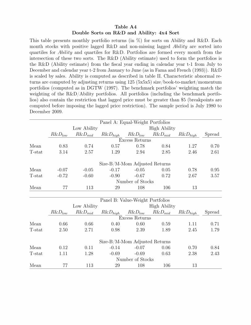
Table A4Double Sorts on R&D and Ability: 4x4 Sort

This table presents monthly portfolio returns (in %) for sorts on Ability and R&D. Eachmonth stocks with positive lagged R&D and non-missing lagged Ability are sorted intoquartiles for Ability and quartiles for R&D. Portfolios are formed every month from theintersection of these two sorts. The R&D (Ability estimate) used to form the portfolios isthe R&D (Ability estimate) from the fiscal year ending in calendar year t-1 from July toDecember and calendar year t-2 from January to June (as in Fama and French (1993)). R&Dis scaled by sales. Ability is computed as described in table II. Characteristic abnormal re-turns are computed by adjusting returns using 125 (5x5x5) size/book-to-market/momentumportfolios (computed as in DGTW (1997). The benchmark portfolios’ weighting match theweighting of the R&D/Ability portfolios. All portfolios (including the benchmark portfo-lios) also contain the restriction that lagged price must be greater than $5 (breakpoints arecomputed before imposing the lagged price restriction). The sample period is July 1980 toDecember 2009.



Mean 0.83 0.74 0.57 0.78 0.84 1.27 0.70T-stat 3.14 2.57 1.29 2.94 2.85 2.46 2.61

Size-B/M-Mom Adjusted ReturnsMean -0.07 -0.05 -0.17 -0.05 0.05 0.78 0.95T-stat -0.72 -0.60 -0.90 -0.67 0.72 2.67 3.57




Mean 0.66 0.66 0.40 0.60 0.59 1.11 0.71T-stat 2.50 2.71 0.98 2.39 1.89 2.45 1.79

Size-B/M-Mom Adjusted ReturnsMean 0.12 0.11 -0.14 -0.07 0.06 0.70 0.84T-stat 1.11 1.28 -0.69 -0.69 0.63 2.38 2.43


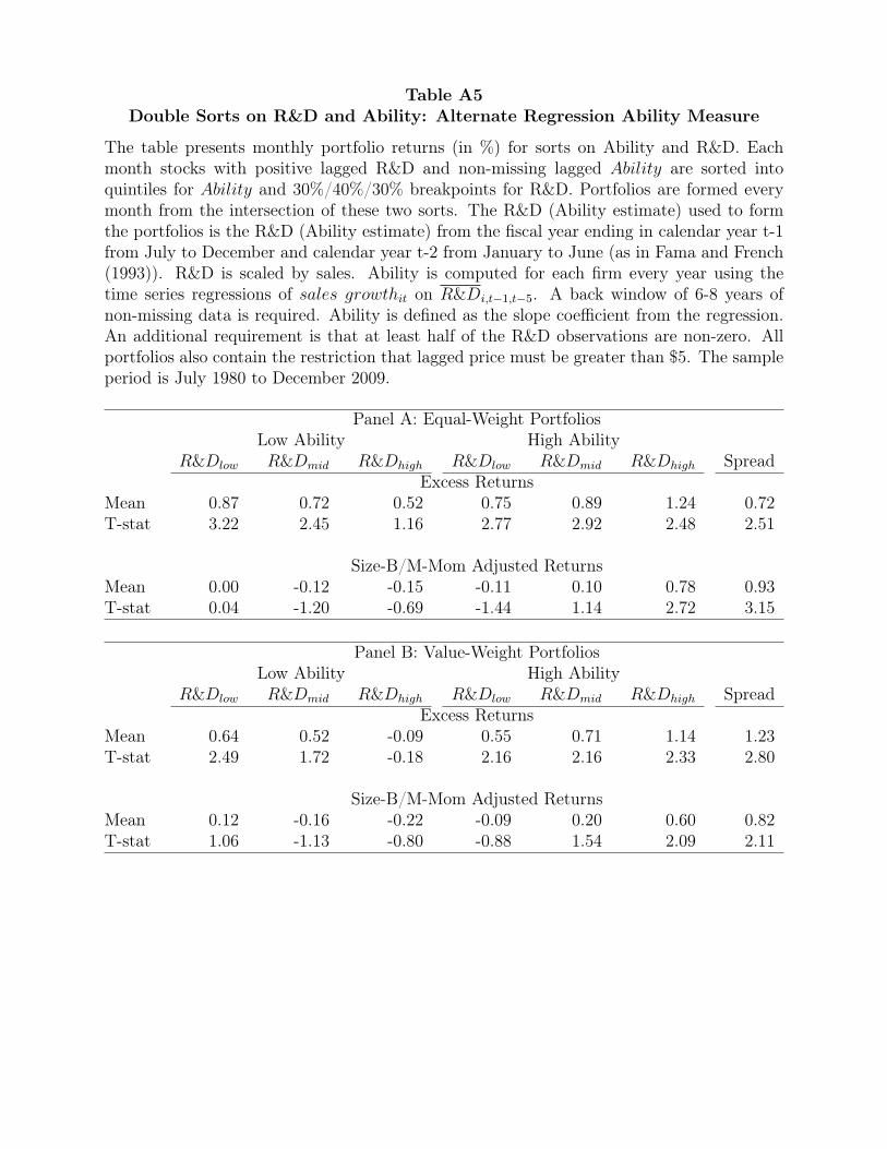
Table A5Double Sorts on R&D and Ability: Alternate Regression Ability Measure

The table presents monthly portfolio returns (in %) for sorts on Ability and R&D. Eachmonth stocks with positive lagged R&D and non-missing lagged Ability are sorted intoquintiles for Ability and 30%/40%/30% breakpoints for R&D. Portfolios are formed everymonth from the intersection of these two sorts. The R&D (Ability estimate) used to formthe portfolios is the R&D (Ability estimate) from the fiscal year ending in calendar year t-1from July to December and calendar year t-2 from January to June (as in Fama and French(1993)). R&D is scaled by sales. Ability is computed for each firm every year using thetime series regressions of sales growthit on R&Di,t−1,t−5. A back window of 6-8 years ofnon-missing data is required. Ability is defined as the slope coefficient from the regression.An additional requirement is that at least half of the R&D observations are non-zero. Allportfolios also contain the restriction that lagged price must be greater than $5. The sampleperiod is July 1980 to December 2009.



Mean 0.87 0.72 0.52 0.75 0.89 1.24 0.72T-stat 3.22 2.45 1.16 2.77 2.92 2.48 2.51




Mean 0.64 0.52 -0.09 0.55 0.71 1.14 1.23T-stat 2.49 1.72 -0.18 2.16 2.16 2.33 2.80


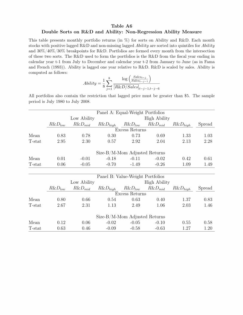
Table A6Double Sorts on R&D and Ability: Non-Regression Ability Measure

This table presents monthly portfolio returns (in %) for sorts on Ability and R&D. Each monthstocks with positive lagged R&D and non-missing lagged Ability are sorted into quintiles for Abilityand 30%/40%/30% breakpoints for R&D. Portfolios are formed every month from the intersectionof these two sorts. The R&D used to form the portfolios is the R&D from the fiscal year ending incalendar year t-1 from July to December and calendar year t-2 from January to June (as in Famaand French (1993)). Ability is lagged one year relative to R&D. R&D is scaled by sales. Ability iscomputed as follows:

Ability =1

8

8∑j=1

log(

Salest−j

Salest−j−1

)[R&D/Sales]t−j−1,t−j−6

All portfolios also contain the restriction that lagged price must be greater than $5. The sampleperiod is July 1980 to July 2008.



Mean 0.83 0.78 0.30 0.73 0.69 1.33 1.03T-stat 2.95 2.30 0.57 2.92 2.04 2.13 2.28

Size-B/M-Mom Adjusted ReturnsMean 0.01 -0.01 -0.18 -0.11 -0.02 0.42 0.61T-stat 0.06 -0.05 -0.70 -1.49 -0.26 1.09 1.49



Mean 0.80 0.66 0.54 0.63 0.40 1.37 0.83T-stat 2.67 2.31 1.13 2.49 1.06 2.03 1.46

Size-B/M-Mom Adjusted ReturnsMean 0.12 0.06 -0.02 -0.05 -0.10 0.55 0.58T-stat 0.63 0.46 -0.09 -0.58 -0.63 1.27 1.20

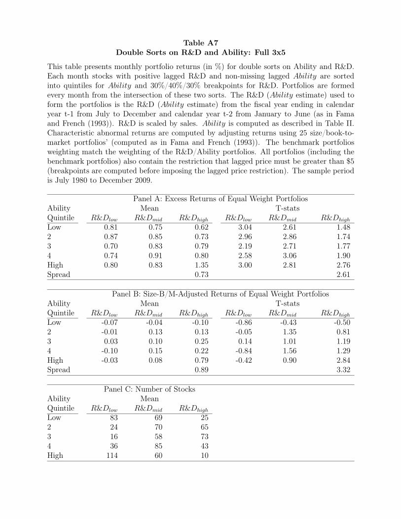
Table A7Double Sorts on R&D and Ability: Full 3x5

This table presents monthly portfolio returns (in %) for double sorts on Ability and R&D.Each month stocks with positive lagged R&D and non-missing lagged Ability are sortedinto quintiles for Ability and 30%/40%/30% breakpoints for R&D. Portfolios are formedevery month from the intersection of these two sorts. The R&D (Ability estimate) used toform the portfolios is the R&D (Ability estimate) from the fiscal year ending in calendaryear t-1 from July to December and calendar year t-2 from January to June (as in Famaand French (1993)). R&D is scaled by sales. Ability is computed as described in Table II.Characteristic abnormal returns are computed by adjusting returns using 25 size/book-to-market portfolios’ (computed as in Fama and French (1993)). The benchmark portfoliosweighting match the weighting of the R&D/Ability portfolios. All portfolios (including thebenchmark portfolios) also contain the restriction that lagged price must be greater than $5(breakpoints are computed before imposing the lagged price restriction). The sample periodis July 1980 to December 2009.

Panel A: Excess Returns of Equal Weight PortfoliosAbility Mean T-statsQuintile R&Dlow R&Dmid R&Dhigh R&Dlow R&Dmid R&Dhigh

Low 0.81 0.75 0.62 3.04 2.61 1.482 0.87 0.85 0.73 2.96 2.86 1.743 0.70 0.83 0.79 2.19 2.71 1.774 0.74 0.91 0.80 2.58 3.06 1.90High 0.80 0.83 1.35 3.00 2.81 2.76Spread 0.73 2.61

Panel B: Size-B/M-Adjusted Returns of Equal Weight PortfoliosAbility Mean T-statsQuintile R&Dlow R&Dmid R&Dhigh R&Dlow R&Dmid R&Dhigh

Low -0.07 -0.04 -0.10 -0.86 -0.43 -0.502 -0.01 0.13 0.13 -0.05 1.35 0.813 0.03 0.10 0.25 0.14 1.01 1.194 -0.10 0.15 0.22 -0.84 1.56 1.29High -0.03 0.08 0.79 -0.42 0.90 2.84Spread 0.89 3.32

Panel C: Number of StocksAbility MeanQuintile R&Dlow R&Dmid R&Dhigh

Low 83 69 252 24 70 653 16 58 734 36 85 43High 114 60 10

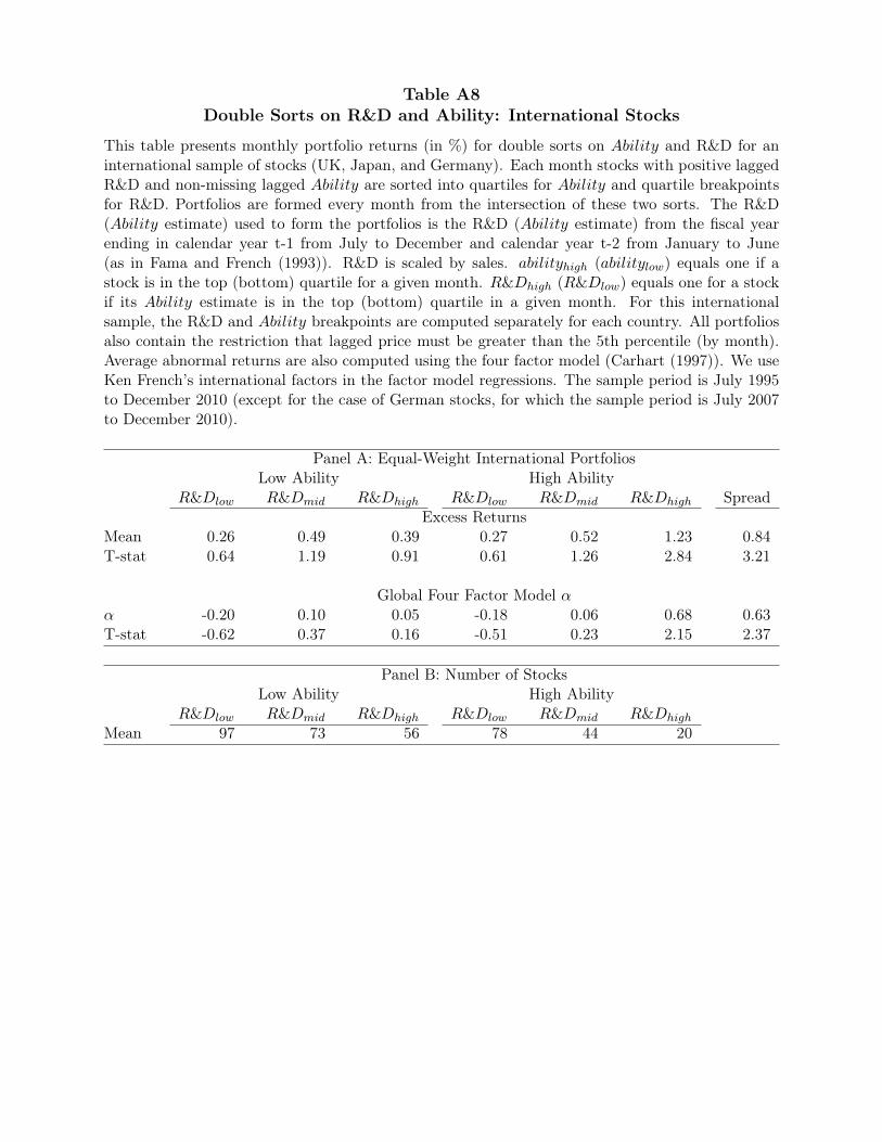
Table A8Double Sorts on R&D and Ability: International Stocks

This table presents monthly portfolio returns (in %) for double sorts on Ability and R&D for aninternational sample of stocks (UK, Japan, and Germany). Each month stocks with positive laggedR&D and non-missing lagged Ability are sorted into quartiles for Ability and quartile breakpointsfor R&D. Portfolios are formed every month from the intersection of these two sorts. The R&D(Ability estimate) used to form the portfolios is the R&D (Ability estimate) from the fiscal yearending in calendar year t-1 from July to December and calendar year t-2 from January to June(as in Fama and French (1993)). R&D is scaled by sales. abilityhigh (abilitylow) equals one if astock is in the top (bottom) quartile for a given month. R&Dhigh (R&Dlow) equals one for a stockif its Ability estimate is in the top (bottom) quartile in a given month. For this internationalsample, the R&D and Ability breakpoints are computed separately for each country. All portfoliosalso contain the restriction that lagged price must be greater than the 5th percentile (by month).Average abnormal returns are also computed using the four factor model (Carhart (1997)). We useKen French’s international factors in the factor model regressions. The sample period is July 1995to December 2010 (except for the case of German stocks, for which the sample period is July 2007to December 2010).

Panel A: Equal-Weight International PortfoliosLow Ability High Ability


Mean 0.26 0.49 0.39 0.27 0.52 1.23 0.84T-stat 0.64 1.19 0.91 0.61 1.26 2.84 3.21

Global Four Factor Model αα -0.20 0.10 0.05 -0.18 0.06 0.68 0.63T-stat -0.62 0.37 0.16 -0.51 0.23 2.15 2.37

Panel B: Number of StocksLow Ability High Ability

R&Dlow R&Dmid R&Dhigh R&Dlow R&Dmid R&Dhigh

Mean 97 73 56 78 44 20

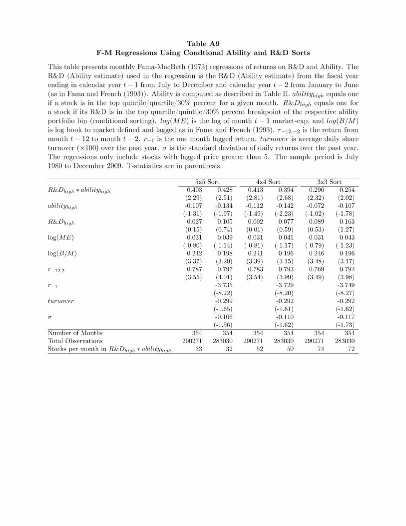
Table A9F-M Regressions Using Condtional Ability and R&D Sorts

This table presents monthly Fama-MacBeth (1973) regressions of returns on R&D and Ability. TheR&D (Ability estimate) used in the regression is the R&D (Ability estimate) from the fiscal yearending in calendar year t− 1 from July to December and calendar year t− 2 from January to June(as in Fama and French (1993)). Ability is computed as described in Table II. abilityhigh equals oneif a stock is in the top quintile/quartile/30% percent for a given month. R&Dhigh equals one fora stock if its R&D is in the top quartile/quintile/30% percent breakpoint of the respective abilityportfolio bin (conditional sorting). log(ME) is the log of month t − 1 market-cap, and log(B/M)is log book to market defined and lagged as in Fama and French (1993). r−12,−2 is the return frommonth t− 12 to month t− 2. r−1 is the one month lagged return. turnover is average daily shareturnover (×100) over the past year. σ is the standard deviation of daily returns over the past year.The regressions only include stocks with lagged price greater than 5. The sample period is July1980 to December 2009. T-statistics are in parenthesis.

5x5 Sort 4x4 Sort 3x3 SortR&Dhigh ∗ abilityhigh 0.403 0.428 0.413 0.394 0.296 0.254

(2.29) (2.51) (2.81) (2.68) (2.32) (2.02)abilityhigh -0.107 -0.134 -0.112 -0.142 -0.072 -0.107

(-1.31) (-1.97) (-1.49) (-2.23) (-1.02) (-1.78)R&Dhigh 0.027 0.105 0.002 0.077 0.089 0.163

(0.15) (0.74) (0.01) (0.59) (0.53) (1.27)log(ME) -0.031 -0.039 -0.031 -0.041 -0.031 -0.043

(-0.80) (-1.14) (-0.81) (-1.17) (-0.79) (-1.23)log(B/M) 0.242 0.198 0.241 0.196 0.246 0.196

(3.37) (3.20) (3.39) (3.15) (3.48) (3.17)r−12,2 0.787 0.797 0.783 0.793 0.769 0.792

(3.55) (4.01) (3.54) (3.99) (3.49) (3.98)r−1 -3.735 -3.729 -3.749

(-8.22) (-8.20) (-8.27)turnover -0.299 -0.292 -0.292

(-1.65) (-1.61) (-1.62)σ -0.106 -0.110 -0.117

(-1.56) (-1.62) (-1.73)Number of Months 354 354 354 354 354 354Total Observations 290271 283030 290271 283030 290271 283030Stocks per month in R&Dhigh ∗ abilityhigh 33 32 52 50 74 72

misvaluing innovation* - hbs people spacemisvaluing innovation — page 1 firms engage in a...

Documents