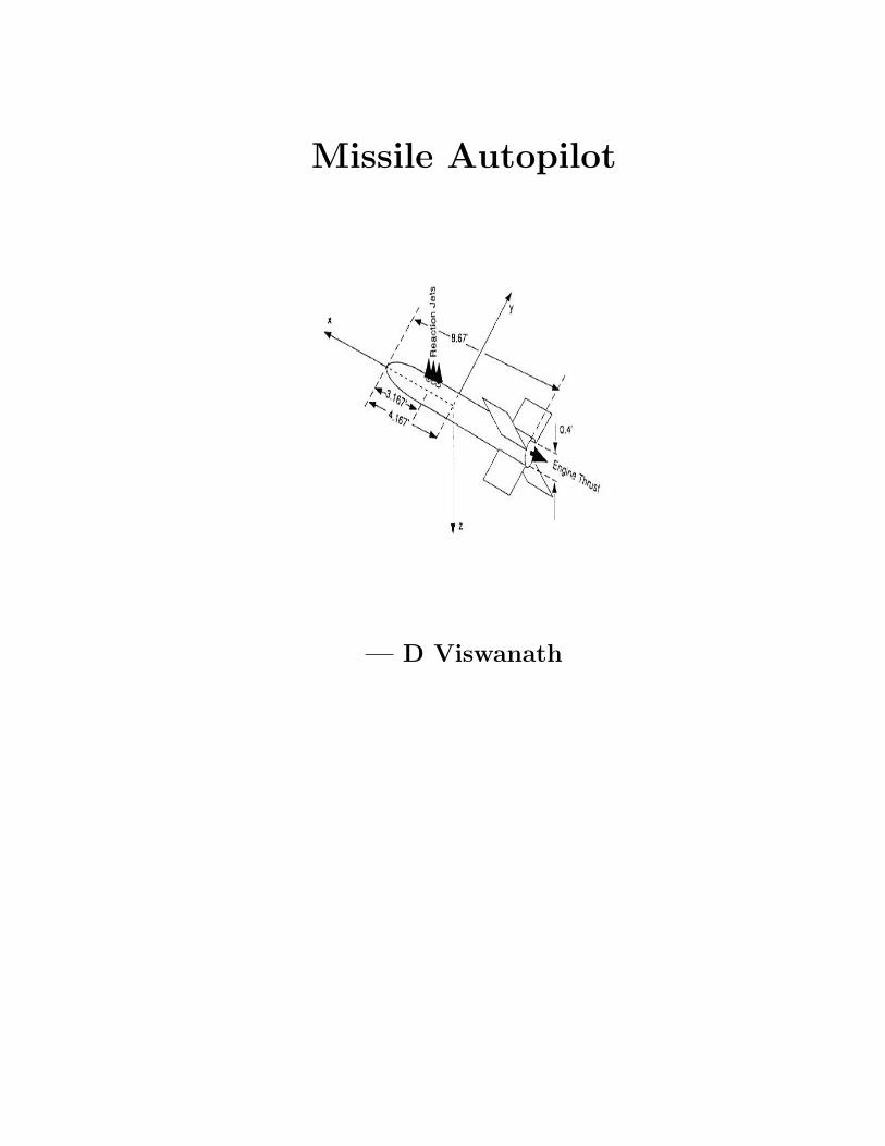
Missile Autopilot

— D Viswanath

Acknowledgment

I am most grateful to my Dr. S. E. Talole, for introducing me to this subject. His

teachings have been my source of motivation throughout this work.

(D Viswanath)

Jan 2011

1

Synopsis

Broadly speaking autopilots either control the motion in the pitch and yaw planes, in

which they are called lateral autopilots, or they control the motion about the fore and

aft axis in which case they are called roll autopilots. Lateral ”g” autopilots are designed

to enable a missile to achieve a high and consistent ”g” response to a command. They

are particularly relevant to SAMs and AAMs. There are normally two lateral autopilots,

one to control the pitch or up-down motion and another to control the yaw or left-right

motion.

The requirements of a good lateral autopilot are very nearly the same for command

and homing systems but it is more helpful initially to consider those associated with

command systems where guidance receiver produces signals proportional to the mis-

alignment of the missile from the line of sight (LOS).

2

Contents

Acknowledgment 1

Synopsis 2

Contents 3

1 Introduction 1

1.1 Overview . . . . . . . . . . . . . . . . . . . . . . . . . . . . . . . . . . . . 2

1.2 Lateral Autopilot Design Objectives . . . . . . . . . . . . . . . . . . . . . 4

1.2.1 Maintenance of near-constant steady state aerodynamic gain . . . 4

1.2.2 Increase weathercock frequency . . . . . . . . . . . . . . . . . . . 5

1.2.3 Increase weathercock damping . . . . . . . . . . . . . . . . . . . . 5

1.2.4 Reduce cross coupling between pitch and yaw motion . . . . . . . 6

1.2.5 Assistance in gathering . . . . . . . . . . . . . . . . . . . . . . . . 6

2 Mathematical Modelling :

Aerodynamic Derivatives and Transfer Functions 7

2.1 Notations and Conventions . . . . . . . . . . . . . . . . . . . . . . . . . . 7

2.2 Equations of Motion . . . . . . . . . . . . . . . . . . . . . . . . . . . . . 10

2.2.1 Euler’s Equations . . . . . . . . . . . . . . . . . . . . . . . . . . . 11

3

2.3 Inertial Form of Force Equation in terms of Eulerian Axes . . . . . . . . 13

2.4 Inertial Form of Moment Equation in terms of Eulerian Axes . . . . . . . 15

2.5 Mathematical Modeling for Missile Lateral Autopilots . . . . . . . . . . . 17

2.5.1 Linearising Moment Equations . . . . . . . . . . . . . . . . . . . . 18

2.5.2 Linearising Force Equations . . . . . . . . . . . . . . . . . . . . . 20

2.6 Translational and Rotational Dynamics of Missile Autopilot . . . . . . . 22

2.6.1 Dynamics of Yaw Autopilot . . . . . . . . . . . . . . . . . . . . . 22

2.6.2 Dynamics of Pitch Autopilot . . . . . . . . . . . . . . . . . . . . . 22

2.6.3 Dynamics of Roll Autopilot . . . . . . . . . . . . . . . . . . . . . 23

2.7 Summary . . . . . . . . . . . . . . . . . . . . . . . . . . . . . . . . . . . 23

2.8 Kinematics of the Missile . . . . . . . . . . . . . . . . . . . . . . . . . . . 23

References 25

4

Chapter 1

Introduction

Broadly speaking autopilots either control the motion in the pitch and yaw planes, in

which they are called lateral autopilots, or they control the motion about the fore and

aft axis in which case they are called roll autopilots.

(a) Lateral ”g” autopilots are designed to enable a missile to achieve a high and con-

sistent ”g” response to a command.

(b) They are particularly relevant to SAMs and AAMs.

(c) There are normally two lateral autopilots, one to control the pitch or up-down

motion and another to control the yaw or left-right motion.

(d) They are usually identical and hence a yaw autopilot is explained here.

(e) An accelerometer is placed in the yaw plane of the missile, to sense the sideways

acceleration of the missile. This accelerometer produces a voltage proportional to

the linear acceleration.

(f) This measured acceleration is compared with the ’demanded’ acceleration.

(g) The error is then fed to the fin servos, which actuate the rudders to move the

missile in the desired direction.

(h) This closed loop system does not have an amplifier, to amplify the error. This is

because of the small static margin in the missiles and even a small error (unam-

plified) provides large airframe movement.

1

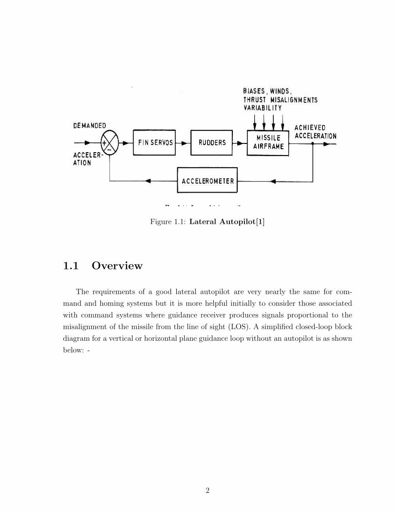
Figure 1.1: Lateral Autopilot[1]

1.1 Overview

The requirements of a good lateral autopilot are very nearly the same for com-

mand and homing systems but it is more helpful initially to consider those associated

with command systems where guidance receiver produces signals proportional to the

misalignment of the missile from the line of sight (LOS). A simplified closed-loop block

diagram for a vertical or horizontal plane guidance loop without an autopilot is as shown

below: -

2

Figure 1.2: Basic Guidance and Control System [1]

(a) The target tracker determines the target direction θt.

(b) Let the guidance receiver gain be K1 volts/rad (misalignment). The guidance

signals are then invariably phase advanced to ensure closed loop stability.

(c) In order to maintain constant sensitivity to missile linear displacement from the

LOS, the signals are multiplied by the measured or assumed missile range Rm

before being passed to the missile servos. This means that the effective d.c. gain

of the guidance error detector is K1 volts/m.

(d) If the missile servo gain is K2 rad/volt and the control surfaces and airframe

produce a steady state lateral acceleration of K3 m/s2/rad then the guidance loop

has a steady state open loop gain of K1K2K3 m/s2/m or K1K2K3 s

−2.

(e) The loop is closed by two inherent integrations from lateral acceleration to lateral

position. Since the error angle is always very small, one can say that the change in

angle is this lateral displacement divided by the instantaneous missile range Rm.

(f) The guidance loop has a gain which is normally kept constant and consists of the

product of the error detector gain, the servo gain and the aerodynamic gain.

3

Consider now the possible variation in the value of aerodynamic gain K3 due to change

in static margin. The c.g. can change due to propellant consumption and manufacturing

tolerances while changes in c.p. can be due to changes in incidence, missile speed and

manufacturing tolerances. The value of K3 can change by a factor of 5 to 1 for changes

in static margin (say 2cm to 10 cm in a 2m long missile). If, in addition, there can be

large variations in the dynamic pressure 12ρu2 due to changes in height and speed, then

the overall variation in aerodynamic gain could easily exceed 100 to 1.

1.2 Lateral Autopilot Design Objectives

The main objectives of a lateral autopilot are as listed below: -

(a) Maintenance of near-constant steady state aerodynamic gain.

(b) Increase weathercock frequency.

(c) Increase weathercock damping.

(d) Reduce cross-coupling between pitch and yaw motion and

(e) Assistance in gathering.

1.2.1 Maintenance of near-constant steady state aerodynamic

gain

A general conclusion can be drawn that an open-loop missile control system is not

acceptable for highly maneuverable missiles, which have very small static margins espe-

cially those which do not operate at a constant height and speed. In homing system,

the performance is seriously degraded if the ”kinematic gain” varies by more than about

+/ − 30 per cent of an ideal value. Since the kinematic gain depends on the control

system gain, the homing head gain and the missile-target relative velocity, and the latter

may not be known very accurately, it is not expected that the missile control designer

will be allowed a tolerance of more than +/− 20 per cent.

4

1.2.2 Increase weathercock frequency

A high weathercock frequency is essential for the stability of the guidance loop.

(a) Consider an open loop system. Since the rest of the loop consists essentially of

two integrations and a d.c. gain, it follows that if there are no dynamic lags in the

loop whatsoever we have 180 deg phase lag at all frequencies open loop.

(b) To obtain stability, the guidance error signal can be passed through phase advance

networks. If one requires more than about 60 degrees phase advance one has to use

several phase advance networks in series and the deterioration in signal-to-noise

ratio is inevitable and catastrophic.

(c) Hence normally designers tend to limit the amount of phase advance to about 60

deg. This means that if one is going to design a guidance loop with a minimum

of 45 deg phase margin, the total phase lag permissible from the missile servo and

the aerodynamics at guidance loop unity gain cross-over frequency will be 15 deg.

(d) Hence the servo must be very much faster and likewise the weathercock frequency

should be much faster (say by a factor of five or more) than the guidance loop

undamped natural frequency i.e., the open-loop unity gain cross-over frequency.

(e) This may not be practicable for an open-loop system especially at the lower end

of the missile speed range and with a small static margin. Hence the requirement

of closed loop system with lateral autopilot arises.

1.2.3 Increase weathercock damping

The weathercock mode is very under-damped, especially with a large static margin and

at high altitudes. This may result in following: -

(a) A badly damped oscillatory mode results in a large r.m.s. output to broadband

noise. The r.m.s. incidence is unnecessarily large and this results in a significant

reduction in range due to induced drag. The accuracy of the missile will also be

degraded.

5

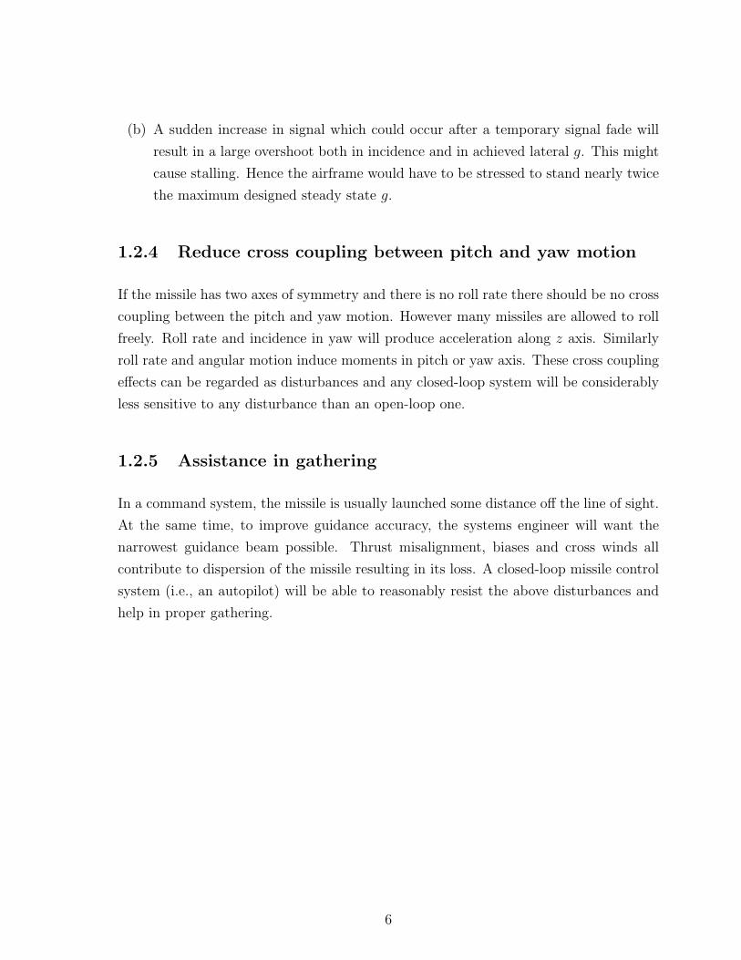
(b) A sudden increase in signal which could occur after a temporary signal fade will

result in a large overshoot both in incidence and in achieved lateral g. This might

cause stalling. Hence the airframe would have to be stressed to stand nearly twice

the maximum designed steady state g.

1.2.4 Reduce cross coupling between pitch and yaw motion

If the missile has two axes of symmetry and there is no roll rate there should be no cross

coupling between the pitch and yaw motion. However many missiles are allowed to roll

freely. Roll rate and incidence in yaw will produce acceleration along z axis. Similarly

roll rate and angular motion induce moments in pitch or yaw axis. These cross coupling

effects can be regarded as disturbances and any closed-loop system will be considerably

less sensitive to any disturbance than an open-loop one.

1.2.5 Assistance in gathering

In a command system, the missile is usually launched some distance off the line of sight.

At the same time, to improve guidance accuracy, the systems engineer will want the

narrowest guidance beam possible. Thrust misalignment, biases and cross winds all

contribute to dispersion of the missile resulting in its loss. A closed-loop missile control

system (i.e., an autopilot) will be able to reasonably resist the above disturbances and

help in proper gathering.

6

Chapter 2

Mathematical Modelling :

Aerodynamic Derivatives and

Transfer Functions

2.1 Notations and Conventions

The reference axis system standardized in the guided weapons industry is centred

on the c.g. and fixed in the body as shown in the figure below:

Figure 2.1: Missile Axes [2]

7

(a) x axis, called the roll axis, forwards, along the axis of symmetry if one exists, but

in any case in the plane of symmetry.

(b) y axis called the pitch axis, outwards and to the right if viewing the missile from

behind

(c) z axis, called the yaw axis, downwards in the plane of symmetry to form a right

handed orthogonal system with the other two.

Thus the missile has six degrees of freedom which consists of three translations and

three rotations along the three body axes as shown in figure below:-

Figure 2.2: Missile Axes Depicting Six Degrees of Freedom[2]

8

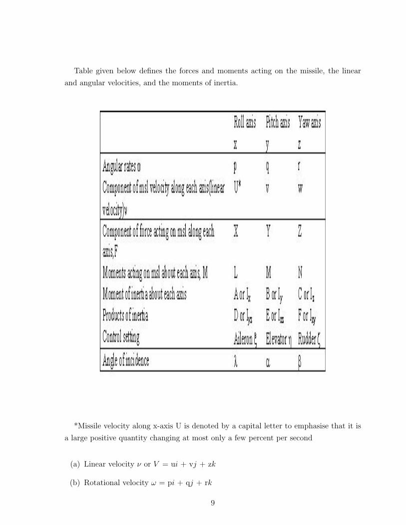
Table given below defines the forces and moments acting on the missile, the linear

and angular velocities, and the moments of inertia.

*Missile velocity along x-axis U is denoted by a capital letter to emphasise that it is

a large positive quantity changing at most only a few percent per second

(a) Linear velocity ν or V = ui + vj + zk

(b) Rotational velocity ω = pi + qj + rk

9

(c) Force F = Xi + Yj + Zk

(d) Moments M = Li + Mj + Nk

(e) Moments of inertia Ix =∫

(y2 + z2) dm = Σ(y2i + z2

i )mi

(f) Products of inertia Iyz =∫yz dM (when body not symmetrical).

2.2 Equations of Motion

The equations of motion of a missile with controls fixed may be derived from Newton’s

second law of motion, which states that the rate of change of momentum of a body is

proportional to the summation of forces applied to the body and that the rate of change

of the moment of momentum is proportional to the summation of moments applied to

the body. Mathematically, this law of motion may be written as (Reference axis can be

taken as the inertial axis (fixed) x,y,z): -

(a) Summation of Forces

ΣFx =d(mU)

dt(2.1)

ΣFy =d(mV )

dt

ΣFz =d(mW )

dt

(b) Summation of Moments

ΣMx =d(hx)

dt(2.2)

ΣMy =d(hy)

dt

ΣMz =d(hz)

dt

where hx, hy, hz are moments of momentum about x, y and z and may be written

in terms of moments of inertia and products of inertia and angular velocities p,q

10

and r of the missile as follows: -

hx = pIx − qIxy − rIxz (2.3)

hy = qIy − rIyz − pIxy

hz = rIz − pIxz − qIyz

For designing an autopilot, we can consider a particular point in space instead of

considering the complete trajectory (system parameters will not be the same at different

points of the trajectory). In that case, mass can be assumed as constant. Hence the

force equations can be rewritten as

ΣF = mdV

dt(2.4)

where V = ui+ vj + wk.

2.2.1 Euler’s Equations

The equations of motion as per Newton’s laws of motion for translational system are

written about an inertial or fixed axis. They are extremely cumbersome and must be

modified before the motion of the missile can be conveniently analysed. In eqn (1), if

i, j and k are considered as not varying with time, then Newton’s law will no longer be

valid since i, j and k with respect to missile body frame change with time. Hence there

is a requirement for expressing the orientation of the fixed axis co-ordinate system with

respect to another moving axis co-ordinate system i.e., co-ordinate transformations need

to be applied. The moving-axis system called the Eulerian axes or Body axis (for

rotational system) is commonly used. This axis system is a right-handed system of

orthogonal coordinate axes whose origin is at the center of gravity of the missile and

whose orientation is fixed with respect to the missile. The Euler angles are designated

as roll (φ), pitch (θ) and yaw (ψ) and are as shown in the figure below:-

11

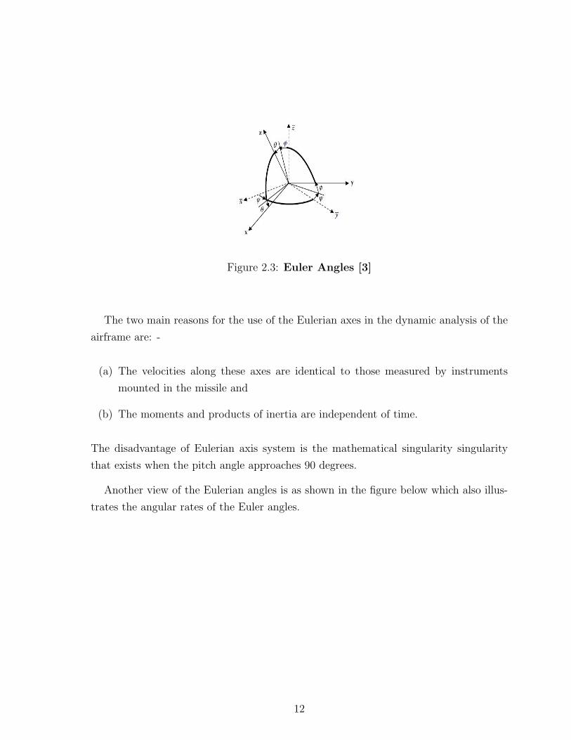
Figure 2.3: Euler Angles [3]

The two main reasons for the use of the Eulerian axes in the dynamic analysis of the

airframe are: -

(a) The velocities along these axes are identical to those measured by instruments

mounted in the missile and

(b) The moments and products of inertia are independent of time.

The disadvantage of Eulerian axis system is the mathematical singularity singularity

that exists when the pitch angle approaches 90 degrees.

Another view of the Eulerian angles is as shown in the figure below which also illus-

trates the angular rates of the Euler angles.

12

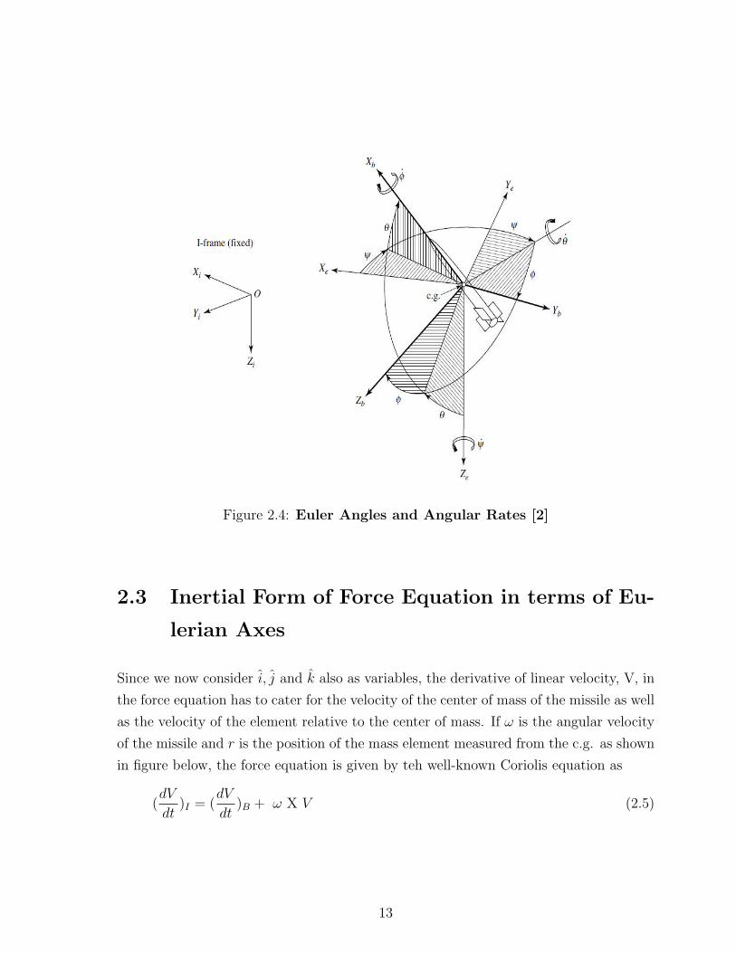
Figure 2.4: Euler Angles and Angular Rates [2]

2.3 Inertial Form of Force Equation in terms of Eu-

lerian Axes

Since we now consider i, j and k also as variables, the derivative of linear velocity, V, in

the force equation has to cater for the velocity of the center of mass of the missile as well

as the velocity of the element relative to the center of mass. If ω is the angular velocity

of the missile and r is the position of the mass element measured from the c.g. as shown

in figure below, the force equation is given by teh well-known Coriolis equation as

(dV

dt)I = (

dV

dt)B + ω X V (2.5)

13

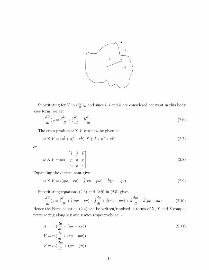
Substituting for V in (dVdt

)B and since i, j and k are considered constant in this body

axes form, we get

(dV

dt)B = i

du

dt+ j

dv

dt+ k

dw

dt(2.6)

The cross-product ω X V can now be given as

ω X V = (pi+ qj + rk) X (ui+ vj + zk) (2.7)

or

ω X V = det

i j k

p q r

u v w

(2.8)

Expanding the determinant gives

ω X V = i(qw − rv) + j(ru− pw) + k(pv − qu) (2.9)

Substituting equations (2.6) and (2.9) in (2.5) gives

(dV

dt)I = i

du

dt+ i(qw − rv) + j

dv

dt+ j(ru− pw) + k

dw

dt+ k(pv − qu) (2.10)

Hence the Force equation (2.4) can be written/resolved in terms of X, Y and Z compo-

nents acting along x,y and z axes respectively as: -

X = m(du

dt+ (qw − rv)) (2.11)

Y = m(dv

dt+ (ru− pw))

Z = m(dw

dt+ (pv − qu))

14

2.4 Inertial Form of Moment Equation in terms of

Eulerian Axes

The moments acting on a body are equal to the rate of change of angular momentum

that is given by

M = (dH

dt)I (2.12)

Angular momentum is equal to the moment of linear momentum whereas the linear

momentum is product of mass and velocity where velocity for a rotating mass is the vec-

tor cross product of angular velocity (ω ) and distance from c.g.(r) (Coriolis Equation).

That is

v = ω X r

Linear Momentum=dm ∗ v=dm ∗ (ω X r)

Angular Momentum (dH)=r X Linear Momentum=r X dm ∗ (ω X r)

Hence

H =

∫(r X (ω X r))dm (2.13)

Considering ω = pi+ qj + rk and r = xi+ yj + zk, their cross product is given by

ω X r = det

i j k

p q r

x y z

(2.14)

Expanding the determinant gives

ω X r = i(qz − ry) + j(rx− pz) + k(py − qx) (2.15)

The vector cross product r X (ω X r) is now given as

r X (ω X r) = det

i j k

x y z

(qz − ry) (rx− pz) (py − qx)

(2.16)

15

Expanding the above determinant gives

r X (ω X r) = [p(y2+z2)−qxy−rxz ]i+[q(x2+z2)−ryz−pxy]j+[r(x2+y2)−pxz−qyz]k

(2.17)

Hence the total angular momentum is given by

H =

∫([p(y2+z2)−qxy−rxz]dmi+[q(x2+z2)−ryz−pxy]dmj+[r(x2+y2)−pxz−qyz]dmk)

(2.18)

Defining the moment of inertia along the x,y and z axes respectively as

Ix =

∫(y2 + z2) dm (2.19)

Iy =

∫(x2 + z2) dm

Iz =

∫(x2 + y2) dm

and similarly

Ixy =

∫(xy) dm (2.20)

Ixz =

∫(xz) dm

Iyz =

∫(yz) dm

the equation for H can be rewritten as

H = [pIx − qIxy − rIxz ]i+ [qIy − rIyz − pIxy]j + [rIz − pIxz − qIyz]k (2.21)

Thus the moment acting on the body

M = (dH

dt)I (2.22)

can also given by

M = (dH

dt)B + (ω X H) (2.23)

16

The term (dHdt

)B is given by

dH

dt)B =

d

dt[pIx− qIxy− rIxz ]i+

d

dt[qIy− rIyz−pIxy]j+

d

dt[rIz−pIxz− qIyz]k (2.24)

and the term ω X H is given by

ω X H = [pi+qj+rk]X [[pIx−qIxy−rIxz ]i+[qIy−rIyz−pIxy]j+[rIz−pIxz−qIyz]k] (2.25)

which can be given by

ω X H =

i j k

p q r

(pIx − qIxy − rIxz) (qIy − rIyz − pIxy) (rIz − pIxz − qIyz)

(2.26)

Expanding the determinant we get

ω X H = i[qrIz − qpIxz − q2Iyz − rqIy + r2Iyz + rpIxy] (2.27)

+j[rpIx − rqIxy − r2Ixz − rpIz + p2Ixz + pqIyz]

+k[pqIy − prIyz − p2Ixy − pqIx + q2Ixy + qrIxz]

Hence the Moment equation can be resolved in terms of L, M and N components acting

along x,y and z axes respectively using

M = (dH

dt)B + (ω X H) (2.28)

and

M = Li+Mj +Nk (2.29)

as: -

L = [pIx + pIx − qIxy − q ˙Ixy − rIxz − r ˙Ixz] + [qrIz − qpIxz − q2Iyz − rqIy + r2Iyz + rpIxy](2.30)

M = [qIy + qIy − rIyz − r ˙Iyz − pIxy − p ˙Ixy] + [rpIx − rqIxy − r2Ixz − rpIz + p2Ixz + pqIyz]

N = [rIz + rIz − pIxz − p ˙Ixz − qIyz − q ˙Iyz] + [pqIy − prIyz − p2Ixy − pqIx + q2Ixy + qrIxz]

2.5 Mathematical Modeling for Missile Lateral Au-

topilots

It is found from the above equations for force and moments, that these are simultaneous

non-linear coupled first order equations that are difficult to solve. Since we are concerned

17

with the design of an autopilot for a missile i.e., math-modelling, we try to linearise these

equations by considering certain basic assumptions.

2.5.1 Linearising Moment Equations

The moment equations are linearised based on the following assumptions:-

(a) Mass is constant. (This has already been considered).

(b) Missile and control surfaces are rigid bodies i.e., they are non-elastic. This is not

always true for control surfaces/wings.(This has been already considered).

(c) C.G. and center of body frame are coincident. This is not true since c.g. keeps

changing as propellant burns and msl moves in angles.(This is already considered).

(d) Rate of change of moment inertia is approximately zero i.e.,Ix, Iy, Iz, Ixy, Ixz, Iyz

are zero. Hence moment equations will simplify as

L = [pIx − qIxy − rIxz] + [qrIz − qpIxz − q2Iyz − rqIy + r2Iyz + rpIxy](2.31)

M = [qIy − rIyz − pIxy] + [rpIx − rqIxy − r2Ixz − rpIz + p2Ixz + pqIyz]

N = [rIz − pIxz − qIyz] + [pqIy − prIyz − p2Ixy − pqIx + q2Ixy + qrIxz]

(e) Missile is symmetrical about xz plane. This is true for aircraft and missiles with

mono-wing configuration (cruise or polar coordinate missiles). In this case, Ixy =

Iyz = 0. Thus moment equations will further simplify as:-

L = [pIx − rIxz] + [qrIz − qpIxz − rqIy] (2.32)

M = [qIy] + [rpIx − r2Ixz − rpIz + p2Ixz]

N = [rIz − pIxz] + [pqIy − pqIx + qrIxz]

This can be simplified as

L = pIx − qr(Iy − Iz)− (pq + r)Ixz (2.33)

M = qIy]− pr(Iz − Ix) + (p2 − r2)Izx

N = rIz − pq(Ix − Iy) + (qr − p)Ixz

18

(f) Missile is symmetrical on xy plane; then Ixz = 0 (in case of cruciform configu-

ration). This will not be true for aircraft and cruise missiles. Thus the moment

equations will further simplify as :-

L = pIx − qr(Iy − Iz) (2.34)

M = qIy]− pr(Iz − Ix)

N = rIz − pq(Ix − Iy)

(g) Consider missile to be a solid cylinder. Then the moment of inertia about y and

z axes will be the same i.e., Iz = Iy. Hence equations will further reduce to:-

L = pIx (2.35)

M = qIy]− pr(Iz − Ix)

N = rIz − pq(Ix − Iy)

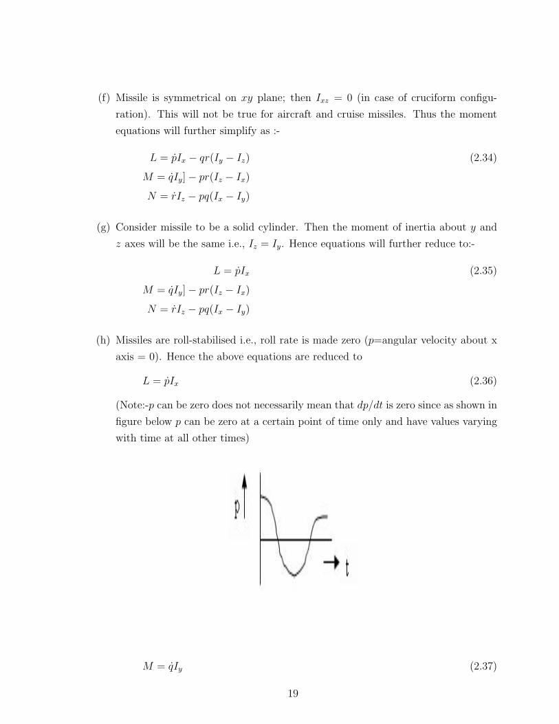
(h) Missiles are roll-stabilised i.e., roll rate is made zero (p=angular velocity about x

axis = 0). Hence the above equations are reduced to

L = pIx (2.36)

(Note:-p can be zero does not necessarily mean that dp/dt is zero since as shown in

figure below p can be zero at a certain point of time only and have values varying

with time at all other times)

M = qIy (2.37)

19

and

N = rIz (2.38)

2.5.2 Linearising Force Equations

The force equations can be linearised based on the following assumptions:-

(a) The Force equation (2.4) resolved in terms of X, Y and Z components acting along

x,y and z axes respectively was derived as: -

X = m(du

dt+ (qw − rv)) (2.39)

Y = m(dv

dt+ (ru− pw))

Z = m(dw

dt+ (pv − qu))

(i) The term mpw in Y is saying that there is a force in the y direction due to

incidence in pitch ( = w/U) and roll motion i.e., there is an acceleration along

y axis due to to roll rate and incidence in pitch. In other words the pitching

motion of the missile is coupled to the yawing motion on account of roll rate.

(ii) The term mpv in Z is also saying that yawing motion induces forces in the

pitch plane if rolling motion is present i.e., acceleration along z axis due to

roll rate and incidence in yaw.

(iii) The presence of the above two terms is most undesirable since we require the

pitch and yaw channels to be completely uncoupled. Cross-coupling between

the planes must contribute to system inaccuracy. To reduce these undesirable

effects the designer tries to keep roll rates as low as possible and in simplified

analysis p is considered zero.

(b) Thus the force equations can be simplified as given below under the assumption

that p is zero:-

X = m(du

dt+ (qw − rv)) (2.40)

Y = m(dv

dt+ ru)

Z = m(dw

dt− qu)

20

(c) The component of velocity in x direction i.e., u also has thrust along its direction

that is of a larger magnitude. Also, this component of velocity will only add to

the thrust in a small way. Hence u is normally written in capital letters to denote

as a constant quantity. Thus the force equations can be written as

X = m(dU

dt+ (qw − rv)) (2.41)

Y = m(dv

dt+ rU)

Z = m(dw

dt− qU)

(d) Thus it is found that the equation for X is of not much use in control system

since the force (thrust) in the x direction does not affect any maneuver; we are

interested in the acceleration perpendicular to the velocity vector as this will result

in a change in the velocity direction. In any case in order to determine the change

in the forward speed we need to know the magnitude of the propulsive and drag

forces.

(e) The forces in y and z direction are responsible for yaw and pitch maneuvers. From

the final equations, it can be seen that the Y and Z equations are linear i.e.,

Y = m(dv

dt+ rU) (2.42)

Z = m(dw

dt− qU)

are linear.

21

2.6 Translational and Rotational Dynamics of Mis-

sile Autopilot

The final simplified equations for forces and moments acting on the missile which rep-

resent the translational and rotational dynamics of the missile respectively are: -

Y = m(dv

dt+ rU) (2.43)

Z = m(dw

dt− qU)

L = pIx

M = qIy

N = rIz

2.6.1 Dynamics of Yaw Autopilot

It can be seen that the equations

Y = m(dv

dt+ rU) (2.44)

N = rIz

are coupled and produce moments about z axis or torque about z axis or the yaw

movement and are used for design of yaw autopilot.

2.6.2 Dynamics of Pitch Autopilot

Similarly the eqns

Z = m(dw

dt− qU) (2.45)

M = qIy

are for pitching dynamics and are used for design of pitch autopilot.

22

2.6.3 Dynamics of Roll Autopilot

The roll autopilot dynamics is represented by the equation

L = pIx (2.46)

2.7 Summary

Thus pitch, yaw and roll dynamics have been decoupled. In other words, a multivariable

system has been decomposed into single variable three sets of equations. This is possible

only in missiles. Design of autopilot for aircraft is much more difficult since this kind of

decoupling is not possible.

2.8 Kinematics of the Missile

The equations for the angular velocities i.e., θ, φ and ψ in terms of the Euler angles roll

(θ), pitch (φ) and (ψ) and the rates p, q and r which are the roll rate, pitch rate and

yaw rate respectively can be resloved from the figure given below:-

Figure 2.5: Euler Angles and Angular Rates [2]

23

θ = q cos φ− r sin φ (2.47)

φ = p+ (q sin φ+ r cos φ)tan θ

ψ = (q sin φ+ r cos φ)sec θ

Thus if x,y and z are the position variables in the fixed frame, they can be related to

u, v and w in the moving frame by the relations as shown below [2]:-xyz

=

cos θ cos ψ sin φ sin θ cos ψ − cos φ sin ψ cos φ sin θ cos ψ + sin φ sin ψ

cos θ sin ψ sin φ sin θ sin ψ + cos φ cos ψ cos φ sin θ sin ψ − sin φ sin ψ−sin θ sin φ cos θ cos φ cos θ

uvw

(2.48)

As can be seen from the above equation, the above transformation can result in

ambiguities or singularities if θ, φ and ψ → 90 degrees. This can be avoided by limiting

the ranges of the Euler angles accordingly.

24

References

[1] P. Garnell, Guided Weapon Control Systems. London: Brassey’s Defence Publishers,

1980.

[2] G. M. Siouris, Missile Guidance and Control Systems. New York: Springer, 2003.

[3] R. Yanushevsky, Modern Missile Guidance. Boca Raton: CRC Press, Taylor Francis

Group, 2008.

25