Mining Collective Intelligence in Diverse Groups

Guo-Jun Qi†, Charu C. Aggarwal‡, Jiawei Han†, Thomas Huang†

†University of Illinois at Urbana-Champaign{qi4, hanj, t-huang1}@illinois.edu

‡IBM T.J. Watson Research Centercharu@us.ibm.com

ABSTRACTCollective intelligence, which aggregates the shared informationfrom large crowds, is often negatively impacted by unreliable infor-mation sources with the low quality data. This becomes a barrierto the effective use of collective intelligence in a variety of appli-cations. In order to address this issue, we propose a probabilisticmodel to jointly assess the reliability of sources and find the truedata. We observe that different sources are often not independentof each other. Instead, sources are prone to be mutually influenced,which makes them dependent when sharing information with eachother. High dependency between sources makes collective intelli-gence vulnerable to the overuse of redundant (and possibly incor-rect) information from the dependent sources. Thus, we reveal thelatent group structure among dependent sources, and aggregate theinformation at the group level rather than from individual sourcesdirectly. This can prevent the collective intelligence from beinginappropriately dominated by dependent sources. We will also ex-plicitly reveal the reliability of groups, and minimize the negativeimpacts of unreliable groups. Experimental results on real-worlddata sets show the effectiveness of the proposed approach with re-spect to existing algorithms.

Categories and Subject DescriptorsH.2.8 [Database applications]: Data mining; Statistical databases

KeywordsCollective intelligence; Crowdsourcing; Robust classifier

1. INTRODUCTIONCollective intelligence aggregates contributions from multiple

sources in order to collect data for a variety of tasks. For example,voluntary participants collaborate with each other to create a fairlyextensive set of entries in Wikipedia, or a crowd of paid personsmay perform image and news article annotations in Amazon Me-chanical Turk. These crowdsourced tasks usually involve multipleobjects, such as Wikipedia entries and images to be annotated. Theparticipating sources collaborate to claim their own observations,such as facts and labels, on these objects. Our goal is to aggregatethese collective observations to infer the true values (e.g., the truefact and image label) for the different objects [18, 14, 5].

We note that an important property of collective intelligence isthat different sources are typically not independent of one another.

Copyright is held by the International World Wide Web ConferenceCommittee (IW3C2). IW3C2 reserves the right to provide a hyperlinkto the author’s site if the Material is used in electronic media.WWW 2013, May 13–17, 2013, Rio de Janeiro, Brazil.ACM 978-1-4503-2035-1/13/05.

For example, in the same social community, people often influ-ence each other, where their judgments and opinions are not inde-pendent. In addition, task participants may obtain their data andknowledge from the same external information source, and theircontributed information will be dependent. Thus, it may not beadvisable to treat sources independently and directly aggregate theinformation from individual sources, when the aggregation processis clearly impacted by such dependencies. In this paper, we willinfer the source dependency by revealing latent group structures a-mong involved sources. Dependent sources will be grouped, andtheir reliability is analyzed at the group level. The incorporation ofsuch dependency analysis in group structures can reduce the riskof overusing the observations made by the dependent sources inthe same group, especially when these observations are unreliable.This helps prevent dependent sources from inappropriately domi-nating collective intelligence especially when these sources are notreliable.

Moreover, we note that groups are not equally reliable, and theymay provide incorrect observations which conflict with each other,either unintentionally or maliciously. Thus, it is important to revealthe reliability of each group, and minimize the negative impact ofthe unreliable groups. For this purpose, we study the general re-liability of each group, as well as its specific reliability on eachindividual object. These two types of reliability are closely relat-ed. General reliability measures the overall performance of a groupby aggregating each individual reliability over the entire set of ob-jects. On the other hand, although each object-specific reliabilityis distinct, it can be better estimated with a prior that a generallyreliable group is likely to be reliable on an individual object andvice versa. Such prior can reduce the overfitting risk of estimatingeach object-specific reliability, especially considering that we needto determine the true value of each object at the same time [11, 1].

The remainder of this paper is organized as follows. We reviewthe related work in Section 2. Our problem and notations are for-mally defined in Section 3. The probabilistic model for the problemis developed in Section 4, followed by a running example that illus-trates the impact of group dependency on the model in Section 5.Section 6 presents the model inference and parameter estimation al-gorithms. Then Section 7 presents the application of the developedmodel to training classifiers from noisy crowdsourced data. We e-valuate the model in Section 8 on real data sets, and summarize thepaper with the conclusion in Section 9.

2. RELATED WORKAggregating crowdsourced knowledge and information has at-

tracted a lot of research efforts, and yields many insightful discov-eries. For example, [16] proposed an iterative truth finder algorith-m by simultaneously accessing the trustworthiness of each source

and the correctness of claimed facts. [1] developed a probabilis-tic graphical model by jointly modeling the abilities of participantsand the correct answers to questions in an aptitude testing setting.The work in [18] developed a latent truth model to infer the sourcequality and correct claims by modeling two types of false positiveand false negative errors of each source. All of these algorithmsestimate the performances of data sources and the impacts on thecredibility of their claimed facts.

However, sources are not independent of each other in real world.Instead, their contributions are typically dependent. [16] noted thisproblem and used a dampening factor to compensate for exces-sively high confidence due to the copied content between sources.But this method did not explicitly model the dependency betweensources, and how the dampening factor can reduce the dependen-cy effect is not clear. On the other hand, [4] studied the relationbetween the content claimed by sources, and developed a separateweighted voting algorithm by considering the copied content be-tween each other. However, the accuracies are accessed indepen-dently on the source level, which can make the accuracy of a datasource overestimated if many other dependent sources repeat thesame false facts.

Moreover, existing models [4, 2, 9, 6] only consider the pairwiserelations between sources to their dependency, which completelyignores the higher-order dependency among sources. In contrast,we explicitly group the dependent sources to capture arbitrary or-ders of dependency among sources. We find that high-order depen-dency prevails in many real cases, and it is more effective to modelthem directly rather than decomposing them into separate pairwiserelations. For example, sources which obtain the content from thesame resource will be assigned to the same group to reflect thehigh order dependency among them. This yields a more compactrepresentation to jointly assess the reliability of data sources andthe correctness of the claimed facts. Moreover, we will see basedon the group-level dependency, independent sources from differentgroups will play more important role than dependent ones in thesame group in inferring the true facts. This is a desired propertywhich can properly aggregate collective knowledge in many realworld tasks.

Modeling the group dependency can be analogized to the com-munity discovery in social networks. Community structure hasbeen considered as a more effective data structure to capture thesocial relations among people than the links between pairs of per-sons [7]. With the similar spirit, the groups can also be more effec-tive than pairwise dependency, and provide deeper insight into theproperty of high-order dependency among sources and how suchproperty affects the aggregation of collective knowledge. Howev-er, it is worth pointing out that the groups defined in our model dif-fer from the communities [3] in social networks. Communities areusually defined as a set of people densely linked in social networks.However, two linked people may not necessarily be influenced byone another when they report the facts and knowledge. Two closefriends can express different opinions and claim conflicting truth-s. Therefore, we will directly investigate the data contributed bysources to find the group structure characterizing their mutual de-pendency that directly affects the source reliability in our collectiveintelligence model.

Finally, our model is motivated to explore the objective facts andknowledge. This is in contrast to the inference of individual’s pref-erence, which aims to recommend products and services based onuser’s ratings and opinions [12]. Instead, in this paper we aim at ag-gregation of collective knowledge to automatically extract the truefacts, such as correct answers to questions and true categories for

S1

S2

S3

S4

O1

O2

O3

S5

y1,1

y2,2

y3,1y3,3

y4,2

y4,3

y5,3

y5,4

Observations

G2

G1

Latent Groups

g1

g2

g3

g4

g5O4

Sources Objects

S5 y5,4g5

O4

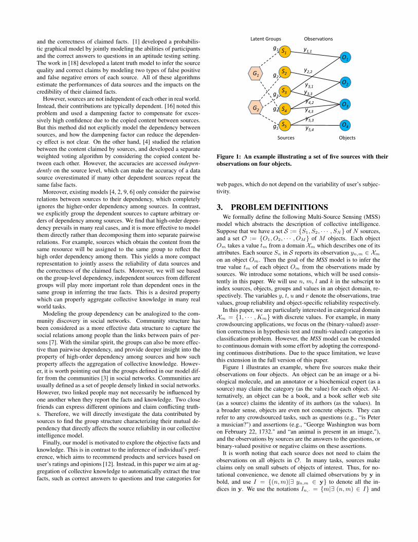
Figure 1: An example illustrating a set of five sources with theirobservations on four objects.

web pages, which do not depend on the variability of user’s subjec-tivity.

3. PROBLEM DEFINITIONSWe formally define the following Multi-Source Sensing (MSS)

model which abstracts the description of collective intelligence.Suppose that we have a set S := {S1, S2, · · · , SN} of N sources,and a set O := {O1, O2, · · · , OM} of M objects. Each objectOm takes a value tm from a domain Xm which describes one of itsattributes. Each source Sn in S reports its observation yn,m ∈ Xm

on an object Om. Then the goal of the MSS model is to infer thetrue value tm of each object Om from the observations made bysources. We introduce some notations, which will be used consis-tently in this paper. We will use n, m, l and k in the subscript toindex sources, objects, groups and values in an object domain, re-spectively. The variables y, t, u and r denote the observations, truevalues, group reliability and object-specific reliability respectively.

In this paper, we are particularly interested in categorical domainXm = {1, · · · ,Km} with discrete values. For example, in manycrowdsourcing applications, we focus on the (binary-valued) asser-tion correctness in hypothesis test and (multi-valued) categories inclassification problem. However, the MSS model can be extendedto continuous domain with some effort by adopting the correspond-ing continuous distributions. Due to the space limitation, we leavethis extension in the full version of this paper.

Figure 1 illustrates an example, where five sources make theirobservations on four objects. An object can be an image or a bi-ological molecule, and an annotator or a biochemical expert (as asource) may claim the category (as the value) for each object. Al-ternatively, an object can be a book, and a book seller web site(as a source) claims the identity of its authors (as the values). Ina broader sense, objects are even not concrete objects. They canrefer to any crowdsourced tasks, such as questions (e.g., “is Petera musician?") and assertions (e.g., “George Washington was bornon February 22, 1732." and “an animal is present in an image,"),and the observations by sources are the answers to the questions, orbinary-valued positive or negative claims on these assertions.

It is worth noting that each source does not need to claim theobservations on all objects in O. In many tasks, sources makeclaims only on small subsets of objects of interest. Thus, for no-tational convenience, we denote all claimed observations by y inbold, and use I = {(n,m)|∃ yn,m ∈ y} to denote all the in-dices in y. We use the notations In,· = {m|∃ (n,m) ∈ I} and

I·,m = {n|∃ (n,m) ∈ I} to denote the subset of indices that areconsistent with the corresponding subscripts n and m.

Meanwhile, in order to model the dependency among sources,we assume that there are a set of latent groups {G1, G2, · · · }, andeach source Sn is assigned to one groupGgn where gn ∈ {1, 2, · · · }is a random variable indicating its membership. For example, as il-lustrated in Figure 1, the five sources are inherently drawn fromtwo latent groups, where each source is linked to the correspondinggroup by dotted lines. Each latent group contains a set of sourceswhich are influenced by each other and tend to make similar ob-servations on objects. The unseen variables of group membershipwill be inferred mathematically from the underlying observation-s. Here, we do not assume any prior knowledge on the numberof groups. The composition of these latent groups will be deter-mined with the use of a Bayesian nonparametric approach by stick-breaking construction [15], as to be presented in the next section.

To minimize the negative impact of unreliable groups, we willexplicitly model the group-level reliability. Specifically, for eachgroup Gl, we define a group reliability score ul ∈ [0, 1] in unitinterval. This value measures the general reliability of the groupover the entire set of objects. A higher value of ul indicates thegreater reliability of the group.

Meanwhile, we also specify the reliability rl,m ∈ {0, 1} of eachgroup Gl on each particular object Om. When rl,m = 1, group Gl

will have reliable performance on Om, and otherwise it will be un-reliable. The reason that we distinguish between reliability ul andobject-specific reliability rl,m is as follows. While a generally reli-able group with a larger value of ul, provides very useful evidenceabout the members of the group on a generic basis, there are likelyto be natural variations within the group itself. Thus, in our model,a group reliability ul only measures how likely it will be reliable onobject set, and whether it will have a reliable performance on a par-ticular object is given by rl,m. In the next section, we will clarifythe relationship between general reliability ul and object-specificreliability rl,m.

4. MULTI-SOURCE SENSING MODELIn this section, we present a generative process for the multi-

source sensing problem. The output of this model will containthe following three aspects: (1) the group membership of sourceswhich describes their dependency when claiming their observationson a set of objects. (2) the reliability ul associated with each groupand its specific reliability rl,m on each object. (3) the true values tmfor each object. Our goal is to reveal the connections between thesethree aspects, especially how the collective observations made bysources can be explained by the latent groups and their reliabilityin a unified probabilistic framework.

First we define the following generative model for multi-sourcesensing (MSS) process below, the details of which will be explainedshortly.

1. Draw λ ∼ GEM(κ) (i.e., stick breaking construction withconcentration κ).

2. For each source Sn,

2.1. Draw its group assignment gn|λ ∼ Discrete(λ);

3. For each object Om,

3.1. Draw its true value tm ∼ Uniform(Xm);

4. For each group Gl:

4.1. Draw its group reliability ul ∼ Beta(b1, b0);

tm

yn,m

πl,m

m=1,…,M

general

reliability

rl,mul,

( )l mr mH t

true value

object-specific

reliability

l=1,…,+∞

n=1,…,N

gn

n,m

group assignment

Figure 2: The graphical model for multi-source sensing. The threeplates represent group reliability ul with l = 1, 2, · · · ,, the truevalues tm for each object Om with m = 1, · · · ,M , and the groupassignment gn of each source with n = 1, · · · , N , respectively.

5. For each pair of group Gl and object Om:

5.1. Draw reliability indicator rl,m ∼ Bernoulli(ul);5.2. Draw the observation model parameter

πl,m|rl,m, tm = z ∼ Hrl,m(tm)

for group Gl on object Om;

6. For each (n,m) ∈ I:

6.1. Draw observation yn,m|πl,m, gn ∼ F (πgn,m);

Here, gn|λ ∼ Discrete(λ) denotes a discrete distribution, whichgenerates the value gn = l with probability λl; H and F are apair of conjugate distributions which are determined by the type ofdata values on objects. For categorical values, these are Dirichletand Multinomial distributions, respectively. Figure 2 illustrates thegenerative process in a graphical representation. We will explainthe details later.

In Step 1, we adopt the stick-breaking construction GEM(κ)(named after Griffiths, Engen and McCloskey) with concentrationparameter κ ∈ R+ to define the prior distribution of assigning eachsource Sn to a latent group Ggn [15]. Specifically, in GEM(κ),a set of random variables ρ = {ρ1, ρ2, · · · } are independentlydrawn from the Beta distribution ρi ∼ Beta(1, κ). They define themixing weights λ of the group membership component such thatp(gn = l|ρ) = λl = ρl

∏l−1i=1 (1− ρi). By the aforementioned

stick-breaking process, we do not need the prior knowledge of thenumber of groups. This number will be determined by capturingthe degree of dependency between sources.

Clearly, we can see that the parameter κ in the above GEM con-struction plays the vital role of determining a priori the degree ofdependency between sources. According to the GEM construction,we can verify that the probability of two sources Sn and Sm beingassigned to the same group is given by the following:

P (gn = gm) =

+∞∑l=1

EλP (gn = l|λ)P (gm = l|λ)

=

+∞∑l=1

Eλl

λ2l =

+∞∑l=1

2

(1 + κ)(2 + κ)

(κ

2 + κ

)l−1

=1

1 + κ

(1)

It is evident that when κ is smaller, sources are more likely to beassigned to the same group where they are dependent and share the

same observation model. This will yield higher degree of depen-dency between sources. As κ increases, the probability that anytwo sources belong to the same group will decrease. In the extremecase, as κ → +∞, this probability approaches zero. In this case,all sources will be assigned to distinctive groups, yielding completeindependence between sources. This shows that the model can flex-ibly capture the various degrees of dependency between sources bysetting an appropriate value of κ.

In Step 3, we adopt the uniform distribution as the prior on thetrue value tm of each object over its domain Xm. The uniformdistribution sets an unbiased prior so that true values will be com-pletely determined a posteriori given observations in the model in-ference. In Section 7, we will show how to set a more informativeprior when more knowledge about objects is available.

In Step 4, we define a Beta distribution Beta(b1, b0) on the groupreliability score ul, where b1 and b0 are the soft counts which spec-ify whether a group is reliable or not a priori, respectively. Then, inStep 5.1, object-specific reliability rl,m ∈ {0, 1} is sampled fromthe Bernoulli distribution Bern(ul) to specify the group reliabilityon a particular objectOm. The higher the general reliability ul, themore likelyGl is reliable on a particular objectOm with rl,m beingsampled to be 1. This suggests that a generally more reliable groupis more likely to be reliable on a particular object. In this sense, thegeneral reliability serves as a prior to reduce the over-fitting risk ofestimating object-specific reliability in the MSS model.

In Step 5.2, the model parameter πl,m for each group on a par-ticular object is drawn from the conjugate prior Hrl,m(tm), whichdepends on the true value tm and the object-specific group relia-bility rl,m. Then, given the group membership gn, each sourceSn generates its observation yn,m according to the correspondinggroup observation model F (πgn,m) in Step 6. In the next subsec-tion, we will detail the specification of Hrl,m(tm) and F (πl,m) incategorical domain.

4.1 Group Observation ModelsIn this subsection, we discuss the specification of group observa-

tion distribution F (πl,m) and its conjugate distributionHrl,m(tm)for categorical values on each object. Here the group observationmodel on each object depends on two factors: (1) the specific re-liability rl,m on this object, which aims to reveal the differencesbetween reliable and unreliable observations on an object, and (2)the true value tm for the object.

It is worth noting that although we distinguish each group obser-vation into reliable and unreliable cases in this subsection, it doesnot mean that two groups are enough to capture the source depen-dency. These two cases are used to model the performance at theobject level. However, given more objects, there are many possiblecombinations of these two cases on different objects. This is whywe need more groups to capture the source dependency based ontheir observations on different objects. In the following, we willdiscuss the group observations models on each object.

In categorical domains, for each group, we choose the multino-mial distribution as its observation model to generate each obser-vation yn,m for its member sources on each object Om. Thus, Step6 in the generative process of MSS model becomes the following:

yn,m|πl,m, gn ∼ F (πgn,m)∆= Multinomial(πgn,m)

where πl,m is the parameter of multinomial distribution for groupGl on object Om. Here, all member sources in the same groupshare the same observation model to capture their dependency.

The model parameter πl,m is generated by the following:

πl,m|rl,m, tm = z ∼ Hrl,m(tm)

∆= Dir(θ(rl,m), · · ·︸ ︷︷ ︸

z−1

, η(rl,m)

↓zth entry

, · · · , θ(rl,m))

where Dir denotes Dirchlet distribution, and θ(rl,m) and η(rl,m) areits soft counts for sampling the false and true values under differentsettings of rl,m.

If group Gl has reliable observations for object Om (i.e., rl,m =1), it should be more likely to sample the true value tm = z as itsobservation than sampling any other false value. Thus, we shouldset a larger value for η(rl,m) than for θ(rl,m).

On the other hand, if group Gl has unreliable observations forobject Om, i.e., rl,m = 0, it should not be more likely to claimthe true value for the object than claiming the false values. There-fore, the group observation model should have η(0) no larger thanθ(0), i.e., η(0) ≤ θ(0). Specifically, the mathematical model candistinguish between uninformative and malicious observations onthe target object:

I. Uninformative observation: When η(0) = θ(0), sources ingroup Gl make uninformative observations on object Om, s-ince false values are equally likely to be claimed as the truevalue. This can be caused when these sources either careless-ly claim their observations at random, or lack the knowledgeabout the target object.

II. Malicious observation: When η(0) < θ(0), it suggests thatthe group Gl contains malicious sources which tend to claimfalse values for object Om. Compared with uninformativeobservations, these malicious observations can even provideus with some information about the target object by inter-preting the observations in a reverse manner. Actually, withθ(0) > η(0), the model gives the unclaimed observation larg-er weight to be evaluated as the true value.

In summary, depending on rl,m, the sources in group Gl makeeither reliable (when rl,m = 1) or unreliable (when rl,m = 0)observations on a particular object Om. Accordingly, the corre-sponding parameters η(rl,m) and θ(rl,m) are constrained in differ-ent ways. When rl,m = 1, we impose a strict inequality η(1) >θ(1) to enforce that group Gl is more likely to claim the true value.On the contrary, when rl,m = 0, we have θ(0) ≥ η(0), representingthat Gl will be unreliable in terms of claiming the true value forOm. In Section 6, we will see how these parameters can be esti-mated by maximizing the observation likelihood of the MSS modelsubject to these constraints.

By putting together these different pieces, the MSS defines acomplete distribution

p(y,g, r,u, t,π|Θ) =M∏

m=1

p(tm)L,M∏

l=1,m=1

p(ul|b1, b0)p(rl,m|ul)

×p(πl,m|rl,m, tm, η(rl,m), θ(rl,m))

×N∏

n=1

p(gn|κ)∏

(n,m)∈I

p(yn,m|gn, πgn,m)

over g = {gn}, r = {rl,m}, u = {ul}, t = {tm}, π ={πl,m} and the source observations y with model parameters Θ =

{η(0), θ(0), η(1), θ(1), b1, b0, κ}. In Section 6, we will present howto infer (1) the true values tm for each object, (2) group assignmentgn of each source, and (3) the general reliability ul of each groupand its specific reliability rl,m on each object from the MSS modela posteriori given the observations y.

0 0

00

0

1

1 1

1

ST

(a) An running example

14 20 40 60−50

−40

−30

−20

−10

0

Number of Independent Sources T

logP (y|H0)logP (y|H1)

(b) Likelihoods of two hypotheses

10 20 30 40 500

101420

30

40

50

Group Size S

(c) Minimal number of independent sources tooverturn the claims by S dependent sources(solid blue curve).

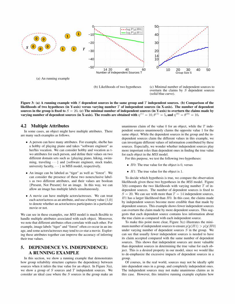
Figure 3: (a) A running example with S dependent sources in the same group and T independent sources. (b) Comparison of thelikelihoods of two hypotheses (in Y-axis) versus varying number T of independent sources (in X-axis). The number of dependentsources in the group is fixed to S = 20. (c) The minimal number of independent sources (in Y-axis) to overturn the claims made byvarying number of dependent sources (in X-axis). The results are obtained with η(1) = 10, θ(1) = 5, and η(0) = θ(0) = 10.

4.2 Multiple AttributesIn some cases, an object might have multiple attributes. There

are many such examples as follows.

• A person can have many attributes. For example, she/he hasa hobby of playing piano and takes “software engineer" asher/his vocation. We can consider hobby and vocation as t-wo attributes for each person, and define their values on twodifferent domain sets such as {playing piano, hiking, swim-ming, traveling · · · } and {software engineer, stock trader,university faculty, · · · } in MSS model, respectively.

• An image can be labeled as “tiger" as well as “forest". Wecan consider the presence of these two nonexclusive label-s as two different attributes, and their values are boolean{Present, Not Present} for an image. In this way, we canallow an image has multiple labels simultaneously.

• A movie can have multiple actors/actresses. We can treateach actor/actress as an attribute, and use a binary value {1,0}to denote whether an actor/actress participates in a particularmovie or not.

We can see in these examples, our MSS model is much flexible tohandle multiple attributes associated with each object. Moreover,we note that different attributes often correlate with each other. Forexample, image labels “tiger" and “forest" often co-occur in an im-age, and some actors/actresses may tend to co-star a movie. Explor-ing these attributes together can improve the accuracy of inferringtheir true values.

5. DEPENDENCE VS. INDEPENDENCE:A RUNNING EXAMPLE

In this section, we show a running example that demonstrateshow group reliability structure captures the dependency betweensources when it infers the true value for an object. In Figure 3(a),we show a group of S sources and T independent sources. Weconsider an ideal case where the S sources in the group make an

unanimous claim of the value 0 for an object, while the T inde-pendent sources unanimously claims the opposite value 1 for thesame object. While the dependent sources in the group and the in-dependent sources claim the different values in this example, wecan investigate different values of information contributed by thesesources. Especially, we wonder whether independent sources playmore important roles than dependent ones in finding the true valuefor each object in the MSS model.

For this purpose, we test the following two hypotheses:

• H0: The true value for the object is 0, versus

• H1: The true value for the object is 1.

To decide which hypothesis is true, we compare the observationlikelihoods given these two hypotheses in the MSS model. Figure3(b) compares the two likelihoods with varying number T of in-dependent sources. The number of dependent sources is fixed toS = 20. We can see with more than T = 14 independent sources,H1 has a larger likelihood than H0. In this case, the claims madeby independent sources become more credible than that made bydependent sources. This example shows fewer independent sourcescan overturn the claim made by more dependent sources. This sug-gests that each dependent source contains less information aboutthe true claim as compared with each independent source.

To make this point more clear, Figure 3(c) illustrates the mini-mum number of independent sources to ensure p(y|H1) > p(y|H0)under varying number of dependent sources S in the group. Wecan see that usually fewer independent sources is needed to haveits claim accepted compared with the same number of dependentsources. This shows that independent sources are more valuablethan dependent sources in determining the true value for each ob-ject. This is a desired property in our model, since we would liketo de-emphasize the excessive impacts of dependent sources in agroup.

Of courses, in the real world, sources may not be ideally splitinto dependent ones in a group, and completely independent ones.The independent sources may not make unanimous claims as inthis case. However, this intuitive running example explains how

the dependency encoded in group structure will affect the inferenceof true value on an object, and illustrates the independent claims aregenerally more valuable than dependent claims in the MSS model.

6. MODEL INFERENCE AND PARAMETERESTIMATION

In this section, we present the inference and learning processes.We wish to infer the tractable posterior p(g, r,u, t,π|y) with aparametric family of variational distributions in the factorized for-m:

q(g, r,u, t,π) =∏n

q(gn|φn)∏l,m

q(rl,m|τ l,m)∏l

q(ul|βl)∏m

q(tm|νm)∏l,m

q(πl,m|αl,m)

with parameters φn, τ l,m, βl, νm and αl,m for these factors. Thedistribution and the parameter for each factor can be determined bythe variational approach [10]. Specifically, we aim to maximize thelower bound of the log likelihood log p(y), i.e.,

log p(y) ≥ Eqlog p(g, r,u, t,π,y)−E

q(log q(g, r,u, t,π))

∆= L(q)

This can obtain the optimal factorized distribution. The lowerbound can be maximized over one factor while the others are fixed.This is an approach which is similar to coordinate descent. In eachiteration, all the factors are updated sequentially over steps by find-ing the fixed-point solutions until convergence. The details of theseupdating steps are provided in Appendix A.

We analyze the computational complexity in one loop of updat-ing all factors. Suppose that we are given N sources, M objects,and obtain L groups by the stick-breaking construction. We alsodenote by Kmax the maximum size of the domain sets among allobjects. Then by investigating the updating steps in Appendix A,we can find that the computational complexity is O(NMLKmax)for one loop.

On the other hand, the model parameters Θ can be estimated bymaximizing the observation likelihood. This can be done by theEM algorithm:E-Step: Given the current parameters in Θ, apply variational infer-ence to obtain the factorization q and their variational parameters;M-Step: Given the factorization q, maximize the lower bound L(q)of the log-likelihood and obtain a new model parameter Θ. (Detailsof this Maximization step are given in Appendix B.)

These two steps are iterated until convergence. We obtain thevariational approximation and the maximum likelihood parameterestimation results simultaneously.

7. CLASSIFICATION PROBLEMSWe are often of particular interest in the classification problem

where each object takes a class as its value from a K-class domainX = {1, 2, · · · ,K}. Moreover, we might be able to access thefeature representations for the objects in O. For example, if the ob-jects are genetic sequences or text documents, we can extract theirfeature descriptors to describe the genetic structure and documentcontent. Therefore, we wish to impose a more informative priorthat aggregates these features into the prior distribution. For thispurpose, given a feature vector xm for an object, the prior on tmbecomes a conditional distribution on xm. For greater modelingflexibility, we choose a distribution for this prior. For example, we

can choose an exponential distribution p(tm|xm,W ):

Exp(W ) := p(tm|xm,W ) =1

Zexp

{K∑

k=1

δ [[tm = k]] ⟨wk,x⟩

}(2)

where each coefficient vector is taken from the parameters W ={wk|k ∈ X}, ⟨wk,x⟩ denotes the inner product between two vec-tors, and Z is the normalization factor to ensure that the above ex-ponential distribution integrates to unit value.

Accordingly, the model inference in Step A.4 in Appendix Ashould be changed. Each updated factor q(tm) in model inferencebecomes an exponential distribution:

q(tm|νm) := exp{K∑

k=1

δ [[tm = k]] νm;k} (3)

with the parameter νm defined as follows:

νm;k = ⟨wk,x⟩+∑l

∑rl

q(rl){(η(rl) − 1)

× Eq(πl,m)

lnπl,m;k +∑k′ ̸=k

(θ(rl) − 1) Eq(πl,m)

lnπl,m;k′}

The other updating steps for the model inference in Appendix Astay the same.

Besides the inference, we need to learn the parameter W inp(tm|xm,W ). Here, we adopt the variational EM (Expectation-Maximization) algorithm. In each iteration, the E-step (expecta-tion) involves computing the tractable posterior distributions as inthe inference step. Then, the maximization step will update W bymaximizing the expected log-likelihood over q as follows:

maxW

M∑m=1

Eq(tm|νm) log p(tm|xm,W ) (4)

We can adopt any off-the-shelf optimization algorithms to solve theabove problem.

The learned parameterized model p(tm|x,W ), as a byproduct, isa classifier conditional on the input feature vector x. This providesus with a way to train a robust classification model with the noisycrowdsourced labels, compared with typical classifiers trained withthe clean labels. On the other hand, the learned classifier enhancesthe MSS model by providing a more discriminative prior of the la-beling information on objects through their feature representations.This regularizes the true classes of objects in the feature space, es-pecially when the classes claimed by different sources on an objectare too scarce or too inconsistent to make robust estimation of thetrue classes. In this case, the imposed prior plays a nontrivial rolein determining the true class of the object.

8. EXPERIMENTAL RESULTSIn this section, we compare our approach with other existing al-

gorithms and demonstrate its effectiveness for inferring source re-liability together with the true values of objects. The comparisonis performed on a book author data set from online book stores,and a user tagging data set from the online image sharing web siteFlickr.com.

8.1 Online Book Store Data SetThe first data set is the book author data set prepared in [16].

The data set is obtained by crawling 1, 263 computer science bookson AbeBooks.com. For each book, AbeBooks.com returns the bookinformation extracted from a set of online book stores. This data set

contains a total of 877 book stores (sources), and 24, 364 listingsof books (objects) and their author lists (object values) reported bythese book stores. Note that each book has a different categoricaldomain that contains all the authors claimed by sources. Our goalis to predict the true authors for each book.

Author names are normalized by preserving the first and lastnames, and ignoring the middle name of each author. For evalu-ation purposes, the authors of 100 books are manually collectedfrom scanned book covers [16]. We compare the returned resultsof each model with the ground truth author lists on this test set andreport the accuracy.

We compare the proposed algorithm MSS with the followingbaselines: (1) the naive voting algorithm which counts the top vot-ed author list for each book as the truth; (2) TruthFinder [16]; (3)Accu [4] which considers the dependency between sources; (4) 2-Estimates as described in [5] with the highest accuracy among allthe models in [5].

Table 3 compares the results of the different algorithms on thebook author data set in terms of the accuracy. The MSS modelachieves the best accuracy among all the compared models. Wenote that the proposed MSS model is an unsupervised algorithmwhich does not involve any training data. In other words, we do notuse any true values in the MSS algorithm in order to produce the re-liability ranking as well as other true values. Even compared withthe accuracy of 0.91 of the Semi-Supervised Truth Finder (SST-F) [17] using extra training data with known true values on someobjects, the MSS model still achieves the highest accuracy of 0.95.

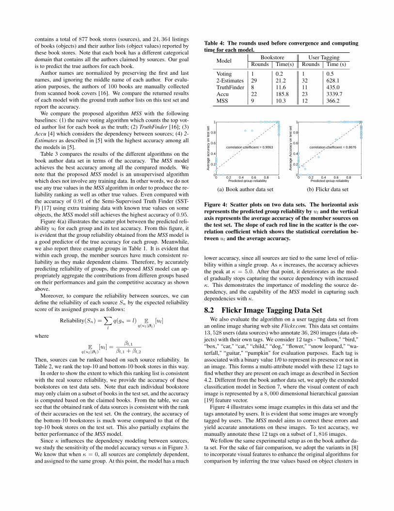
Figure 4(a) illustrates the scatter plot between the predicted reli-ability ul for each group and its test accuracy. From this figure, itis evident that the group reliability obtained from the MSS model isa good predictor of the true accuracy for each group. Meanwhile,we also report three example groups in Table 1. It is evident thatwithin each group, the member sources have much consistent re-liability as they make dependent claims. Therefore, by accuratelypredicting reliability of groups, the proposed MSS model can ap-propriately aggregate the contributions from differen groups basedon their performances and gain the competitive accuracy as shownabove.

Moreover, to compare the reliability between sources, we candefine the reliability of each source Sn by the expected reliabilityscore of its assigned groups as follows:

Reliability(Sn) =∑l

q(gn = l) Eq(ul|βl)

[ul]

where

Eq(ul|βl)

[ul] =βl,1

βl,1 + βl,2

Then, sources can be ranked based on such source reliability. InTable 2, we rank the top-10 and bottom-10 book stores in this way.

In order to show the extent to which this ranking list is consistentwith the real source reliability, we provide the accuracy of thesebookstores on test data sets. Note that each individual bookstoremay only claim on a subset of books in the test set, and the accuracyis computed based on the claimed books. From the table, we cansee that the obtained rank of data sources is consistent with the rankof their accuracies on the test set. On the contrary, the accuracy ofthe bottom-10 bookstores is much worse compared to that of thetop-10 book stores on the test set. This also partially explains thebetter performance of the MSS model.

Since κ influences the dependency modeling between sources,we study the sensitivity of the model accuracy versus κ in Figure 3.We know that when κ = 0, all sources are completely dependent,and assigned to the same group. At this point, the model has a much

Table 4: The rounds used before convergence and computingtime for each model.

Model Bookstore User TaggingRounds Time(s) Rounds Time (s)

Voting 1 0.2 1 0.52-Estimates 29 21.2 32 628.1TruthFinder 8 11.6 11 435.0Accu 22 185.8 23 3339.7MSS 9 10.3 12 366.2

0 0.2 0.4 0.6 0.8 10

0.2

0.4

0.6

0.8

1

Predicted group reliability

Ave

rage

acc

urac

y on

test

set

correlation coefficient = 0.9063

(a) Book author data set

0 0.2 0.4 0.6 0.8 10

0.2

0.4

0.6

0.8

1

Predicted group reliability

Ave

rage

Acc

urac

y on

test

set

correlation coefficient = 0.8676

(b) Flickr data set

Figure 4: Scatter plots on two data sets. The horizontal axisrepresents the predicted group reliability by ul and the verticalaxis represents the average accuracy of the member sources onthe test set. The slope of each red line in the scatter is the cor-relation coefficient which shows the statistical correlation be-tween ul and the average accuracy.

lower accuracy, since all sources are tied to the same level of relia-bility within a single group. As κ increases, the accuracy achievesthe peak at κ = 5.0. After that point, it deteriorates as the mod-el gradually stops capturing the source dependency with increasedκ. This demonstrates the importance of modeling the source de-pendency, and the capability of the MSS model in capturing suchdependencies with κ.

8.2 Flickr Image Tagging Data SetWe also evaluate the algorithm on a user tagging data set from

an online image sharing web site Flickr.com. This data set contains13, 528 users (data sources) who annotate 36, 280 images (data ob-jects) with their own tags. We consider 12 tags - “balloon," “bird,"“box," “car," “cat," “child," “dog," “flower," “snow leopard," “wa-terfall," “guitar," “pumpkin" for evaluation purposes. Each tag isassociated with a binary value 1/0 to represent its presence or not inan image. This forms a multi-attribute model with these 12 tags tofind whether they are present on each image as described in Section4.2. Different from the book author data set, we apply the extendedclassification model in Section 7, where the visual content of eachimage is represented by a 8, 000 dimensional hierarchical gaussian[19] feature vector.

Figure 4 illustrates some image examples in this data set and thetags annotated by users. It is evident that some images are wronglytagged by users. The MSS model aims to correct these errors andyield accurate annotations on these images. To test accuracy, wemanually annotate these 12 tags on a subset of 1, 816 images.

We follow the same experimental setup as on the book author da-ta set. For the sake of fair comparison, we adopt the variants in [8]to incorporate visual features to enhance the original algorithms forcomparison by inferring the true values based on object clusters in

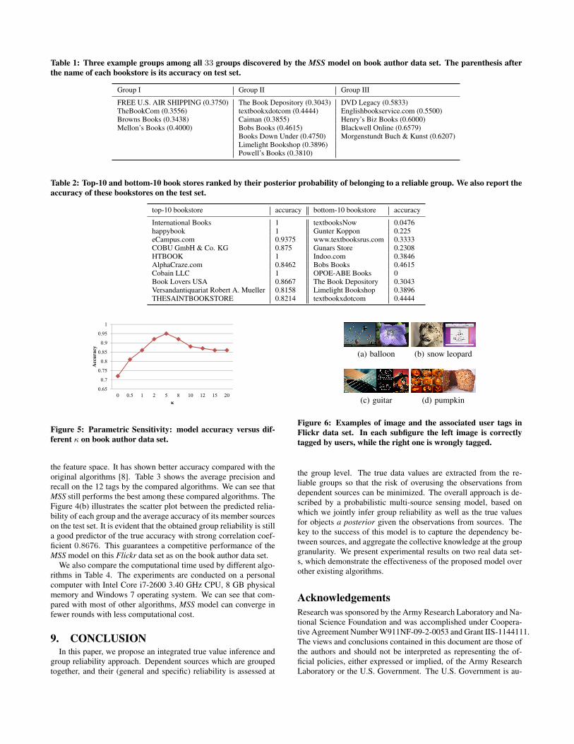
Table 1: Three example groups among all 33 groups discovered by the MSS model on book author data set. The parenthesis afterthe name of each bookstore is its accuracy on test set.

Group I Group II Group III

FREE U.S. AIR SHIPPING (0.3750) The Book Depository (0.3043) DVD Legacy (0.5833)TheBookCom (0.3556) textbookxdotcom (0.4444) Englishbookservice.com (0.5500)Browns Books (0.3438) Caiman (0.3855) Henry’s Biz Books (0.6000)Mellon’s Books (0.4000) Bobs Books (0.4615) Blackwell Online (0.6579)

Books Down Under (0.4750) Morgenstundt Buch & Kunst (0.6207)Limelight Bookshop (0.3896)Powell’s Books (0.3810)

Table 2: Top-10 and bottom-10 book stores ranked by their posterior probability of belonging to a reliable group. We also report theaccuracy of these bookstores on the test set.

top-10 bookstore accuracy bottom-10 bookstore accuracy

International Books 1 textbooksNow 0.0476happybook 1 Gunter Koppon 0.225eCampus.com 0.9375 www.textbooksrus.com 0.3333COBU GmbH & Co. KG 0.875 Gunars Store 0.2308HTBOOK 1 Indoo.com 0.3846AlphaCraze.com 0.8462 Bobs Books 0.4615Cobain LLC 1 OPOE-ABE Books 0Book Lovers USA 0.8667 The Book Depository 0.3043Versandantiquariat Robert A. Mueller 0.8158 Limelight Bookshop 0.3896THESAINTBOOKSTORE 0.8214 textbookxdotcom 0.4444

0.65

0.7

0.75

0.8

0.85

0.9

0.95

1

0 0.5 1 2 5 8 10 12 15 20

Accuracy

κ

Figure 5: Parametric Sensitivity: model accuracy versus dif-ferent κ on book author data set.

the feature space. It has shown better accuracy compared with theoriginal algorithms [8]. Table 3 shows the average precision andrecall on the 12 tags by the compared algorithms. We can see thatMSS still performs the best among these compared algorithms. TheFigure 4(b) illustrates the scatter plot between the predicted relia-bility of each group and the average accuracy of its member sourceson the test set. It is evident that the obtained group reliability is stilla good predictor of the true accuracy with strong correlation coef-ficient 0.8676. This guarantees a competitive performance of theMSS model on this Flickr data set as on the book author data set.

We also compare the computational time used by different algo-rithms in Table 4. The experiments are conducted on a personalcomputer with Intel Core i7-2600 3.40 GHz CPU, 8 GB physicalmemory and Windows 7 operating system. We can see that com-pared with most of other algorithms, MSS model can converge infewer rounds with less computational cost.

9. CONCLUSIONIn this paper, we propose an integrated true value inference and

group reliability approach. Dependent sources which are groupedtogether, and their (general and specific) reliability is assessed at

(a) balloon

(b) snow leopard

(c) guitar

(d) pumpkin

Figure 6: Examples of image and the associated user tags inFlickr data set. In each subfigure the left image is correctlytagged by users, while the right one is wrongly tagged.

the group level. The true data values are extracted from the re-liable groups so that the risk of overusing the observations fromdependent sources can be minimized. The overall approach is de-scribed by a probabilistic multi-source sensing model, based onwhich we jointly infer group reliability as well as the true valuesfor objects a posterior given the observations from sources. Thekey to the success of this model is to capture the dependency be-tween sources, and aggregate the collective knowledge at the groupgranularity. We present experimental results on two real data set-s, which demonstrate the effectiveness of the proposed model overother existing algorithms.

AcknowledgementsResearch was sponsored by the Army Research Laboratory and Na-tional Science Foundation and was accomplished under Coopera-tive Agreement Number W911NF-09-2-0053 and Grant IIS-1144111.The views and conclusions contained in this document are those ofthe authors and should not be interpreted as representing the of-ficial policies, either expressed or implied, of the Army ResearchLaboratory or the U.S. Government. The U.S. Government is au-

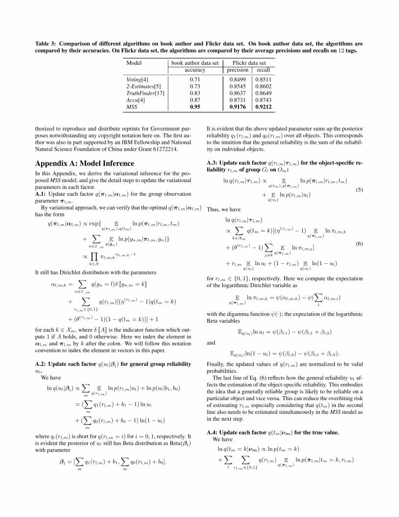
Table 3: Comparison of different algorithms on book author and Flickr data set. On book author data set, the algorithms arecompared by their accuracies. On Flickr data set, the algorithms are compared by their average precisions and recalls on 12 tags.

Model book author data set Flickr data setaccuracy precision recall

Voting[4] 0.71 0.8499 0.85112-Estimates[5] 0.73 0.8545 0.8602TruthFinder[17] 0.83 0.8637 0.8649Accu[4] 0.87 0.8731 0.8743MSS 0.95 0.9176 0.9212

thorized to reproduce and distribute reprints for Government pur-poses notwithstanding any copyright notation here on. The first au-thor was also in part supported by an IBM Fellowship and NationalNatural Science Foundation of China under Grant 61272214.

Appendix A: Model InferenceIn this Appendix, we derive the variational inference for the pro-posed MSS model, and give the detail steps to update the variationalparameters in each factor.A.1: Update each factor q(πl,m|αl,m) for the group observationparameter πl,m.

By variational approach, we can verify that the optimal q(πl,m|αl,m)has the form

q(πl,m|αl,m) ∝ exp{ Eq(rl,m),q(tm)

ln p(πl,m|rl,m, tm)

+∑

n∈I·,m

Eq(gn)

ln p(yn,m|πl,m, gn)}

∝∏k∈X

πl,m;kαl,m;k−1

It still has Dirichlet distribution with the parameters

αl,m;k =∑

n∈I·,m

q(gn = l)δ [[yn,m = k]]

+∑

rl,m∈{0,1}

q(rl,m)[(η(rl,m) − 1)q(tm = k)

+ (θ(rl,m) − 1)(1− q(tm = k))] + 1

for each k ∈ Xm, where δ [[A]] is the indicator function which out-puts 1 if A holds, and 0 otherwise. Here we index the element inαl,m and πl,m by k after the colon. We will follow this notationconvention to index the element in vectors in this paper.

A.2: Update each factor q(ul|βl) for general group reliabilityul.

We have

ln q(ul|βl) ∝∑m

Eq(rl,m)

ln p(rl,m|ul) + ln p(ul|b1, b0)

= (∑m

q1(rl,m) + b1 − 1) lnul

+ (∑m

q0(rl,m) + b0 − 1) ln(1− ul)

where qi(rl,m) is short for q(rl,m = i) for i = 0, 1, respectively. Itis evident the posterior of ul still has Beta distribution as Beta(βl)with parameter

βl = [∑m

q1(rl,m) + b1,∑m

q0(rl,m) + b0].

It is evident that the above updated parameter sums up the posteriorreliability q1(rl,m) and q0(rl,m) over all objects. This correspondsto the intuition that the general reliability is the sum of the reliabil-ity on individual objects.

A.3: Update each factor q(rl,m|τ l,m) for the object-specific re-liability rl,m of group Gl on Om:

ln q(rl,m|τ l,m) ∝ Eq(tm),q(πl,m)

ln p(πl,m|rl,m, tm)

+ Eq(ul)

ln p(rl,m|ul)(5)

Thus, we have

ln q(rl,m|τ l,m)

∝∑

k∈Xm

q(tm = k)[(η(rl,m) − 1) Eq(πl,m)

lnπl,m;k

+ (θ(rl,m) − 1)∑j ̸=k

Eq(πl,m)

lnπl,m;j ]

+ rl,m Eq(ul)

lnul + (1− rl,m) Eq(ul)

ln(1− ul)

(6)

for rl,m ∈ {0, 1}, respectively. Here we compute the expectationof the logarithmic Dirichlet variable as

Eq(πl,m)

lnπl,m;k = ψ(αl,m;k)− ψ(∑i

αl,m;i)

with the digamma function ψ(·); the expectation of the logarithmicBeta variables

Eq(ul)lnul = ψ(βl;1)− ψ(βl;1 + βl;2)

and

Eq(ul)ln(1− ul) = ψ(βl;2)− ψ(βl;1 + βl;2).

Finally, the updated values of q(rl,m) are normalized to be validprobabilities.

The last line of Eq. (6) reflects how the general reliability ul af-fects the estimation of the object-specific reliability. This embodiesthe idea that a generally reliable group is likely to be reliable on aparticular object and vice versa. This can reduce the overfitting riskof estimating rl,m especially considering that q(tm) in the secondline also needs to be estimated simultaneously in the MSS model asin the next step.

A.4: Update each factor q(tm|νm) for the true value.We have

ln q(tm = k|νm) ∝ ln p(tm = k)

+∑l

∑rl,m∈{0,1}

q(rl,m) Eq(πl,m)

ln p(πl,m|tm = k, rl,m)

This suggests that

ln q(tm = k|νm)

∝∑l

∑rl,m

q(rl,m){(η(rl,m) − 1) Eq(πl,m)

lnπl,m;k

+∑k′ ̸=k

(θ(rl,m) − 1) Eq(πl,m)

lnπl,m;k′}

All q(tm = k), k ∈ Xm are normalized to ensure they are validateprobabilities.

A.5: Update each factor q(gn|φn) for the group assignment ofeach source.

We can deriveln q(gn = l|φn)

∝ Eq(ρ)

ln p(gn = l|ρ) +∑

m∈In,·

Eq(πl,m)

ln p(yn,m|πl,m, gn = l)

= Eq(ρ)

ln p(gn = l|ρ) +∑

m∈In,·

Eq(πl,m)

lnπl,m;yn,m

This shows that q(gn = l|φn) is a multinomial distribution withits parameter as

φn;l = q(gn = l|φn) =exp(Un,l)

∞∑l=1

exp(Un,l)(7)

where

Un,l = Eq(ρ)

ln p(gn = l|ρ) +∑

m∈In,·E

q(πl,m)lnπl,m;yn,m

As in [13], we truncate after L groups: the posterior distributionq(ρi) after the level L is set to be its prior p(ρi) from Beta(1, κ);and all the expectations E

q(πl,m)lnπl,m;k after L are set to:

Eq(πl,m) lnπl,m;k = Eq(tm),p(rl,m)

{ E[lnπl,m;k|rl,m, tm] }

with the prior distribution p(rl,m) defined as Section 4 for all l >L, respectively. The inner conditional expectation in the above istaken with respect to the probability of πl,m conditional on rl,mand tm. Similar to the family of nested Dirichlet process mixturein [13], this will form a family of nested priors indexed by L forthe MSS model. Thus, we can compute the infinite sum in the de-nominator of Eq. (7) as:

∞∑l=L+1

exp(Un,l) =exp(Un,L+1)

1− exp( Eρi∼Beta(1,κ)

ln(1− ρi))

A.6: Update q(ρi) in GEM construction.Before the truncation level L, the posterior distribution q(ρi) ∼

Beta(ϕi,1, ϕi,2) is updated as

ϕi,1 = 1 +

N∑n=1

q(gn = i), ϕi,2 = κ+

N∑n=1

∞∑j=i+1

q(gn = j)

Appendix B: Parameter EstimationThe model parameters Θ = {η(0), θ(0), η(1), θ(1), b1, b0, κ} canbe estimated by maximizing the log-likelihood logL(q) by the ob-tained factorization q with the constraints η(1) > θ(1) and η(0) ≤θ(0). Since we require η(1) > θ(1) strictly holds, we usually im-pose η(1) ≥ (1+ϵ)θ(1) with a positive value of ϵ, i.e., η(1) is larger

than θ(1) with a margin ϵ. This ensures the strict inequality and im-proves numerical stability. In the algorithm, we set ϵ = 0.5. Then,the parameter estimation problem becomes the following:

Θ⋆ = argmaxΘ

L(q)

s.t., 0 ≤ η(0) ≤ θ(0), η(1) ≥ (1 + ε)θ(1) ≥ 0,b1, b0, κ ≥ 0

This constrained optimization problem can be solved by many off-the-shelf gradient-based constrained optimization solvers with thefollowing gradients:

∂L∂η(r)

=∑

l,m,k∈Xm

{ψ(η(r) + (Km − 1)θ(r))− ψ(η(r))

+ψ(αl,m;k)− ψ(∑i

αl,m;i)}

∂L∂θ(r)

=∑

k∈Xm

{ψ(η(r) + (Km − 1) θ(r))− (Km − 1)ψ(θ(r))

+∑k′ψ(αl,m;k′)− (Km − 1)ψ(

∑i

αl,m;i)}

for r ∈ {0, 1}.

∂L∂b1

=∑l

ψ(b1 + b0)− ψ(b1) + ψ(βl,1)− ψ(βl,1 + βl,2)

∂L∂b0

=∑l

ψ(b1 + b0)− ψ(b0) + ψ(βl,2)− ψ(βl,1 + βl,2)

∂L∂κ

=∑i

ψ(1 + κ)− ψ(κ) + ψ(ϕi,1 + ϕi,2)− ψ(ϕi,2)

10. REFERENCES[1] Y. Bachrach, T. Minka, J. Guiver, and T. Graepel. How to

grade a test without knowing the answers - a bayesiangraphical model for adaptive crowdsourcing and aptitudetesting. In Proc. of International Conference on MachineLearning, 2012.

[2] M. Bilgic, G. Namata, and L. Getoor. Combining collectiveclassification and link prediction. In Workshop on MiningGraphs and Complex Structures (at ICDM), 2007.

[3] A. Clauset, M. E. J. Newman, and C. Moore. Findingcommunity structure in very large networks. Physical ReviewE, 70:066111, 2004.

[4] X. L. Dong, L. Berti-Equille, and D. Srivastava. Integratingconflicting data: The role of source dependence. In Proc. ofInternational Conference on Very Large Databases, August2009.

[5] A. Galland, S. Abiteboul, A. Marian, and P. Senellart.Corroborating information from disagreeing views. In Proc.of ACM International Conference on Web Search and DataMining, February 2010.

[6] L. Getoor, N. Friedman, D. Koller, and B. Taskar. Learningprobabilistic models of link structure. Journal of MachineLearning Research, (3):679–707, 2002.

[7] M. Girvan and M. Newman. Community structure in socialand biological networks. Proceedings of the NationalAcademy of Sciences, 99(12):7821–7826, June 2002.

[8] M. Gupta, Y. Sun, and J. Han. Trust analysis with clustering.In Proc. of International World Wide Web Conference, April2011.

[9] O. Hassanzadeh and et al. A framework for semantic linkdiscovery over relational data. In CIKM, 2009.

[10] M. Jordan, Z. Ghahramani, T. Jaakkola, and L. Saul.Introduction to variational methods for graphical models.Machine Learning, 37:183–233, 1999.

[11] G. Kasneci, J. V. Gael, D. Stern, and T. Graepel. Cobayes:Bayesian knowledge corroboration with assessors ofunknown areas of expertise. In Proc. of ACM InternationalConference on Web Search and Data Mining, 2011.

[12] Y. Koren, R. Bell, and C. Volinsky. Matrix factorizationtechniques for recommender systems. Computer,42(8):30–37, August 2009.

[13] K. Kurihara, M. Welling, and N. Vlassis. Acceleratedvariational dirichlet process mixtures. In NIPS, 2006.

[14] J. Pasternack and D. Roth. Knowing what to believe (whenyou already know something). In Proc. of InternationalConference on Computational Linguistics, August 2010.

[15] J. Sethuraman. A constructive definition of dirichlet priors.Statistica Sinica, 4:639–650, 1994.

[16] X. Yin, J. Han, and P. S. Yu. Truth discovery with multipleconflicting information providers on the web. In Proc. ofACM SIGKDD conference on Knowledge Discovery andData Mining, August 2007.

[17] X. Yin and W. Tan. Semi-supervised truth discovery. In Proc.of International World Wide Web Conference, March28-April 1 2011.

[18] B. Zhao, B. I. P. Rubinstein, J. Gemmell, and J. Han. Abayesian approach to discovering truth from conflictingsources for data integration. In Proc. of InternationalConference on Very Large Databases, 2012.

[19] X. Zhou, N. Cui, Z. Li, F. Liang, and T. Huang. Hierarchicalgaussianization for image classification, 2009.