microsoft office excel for the public works … ® office excel ® for the public works professional...
TRANSCRIPT

Microsoft® Office Excel® for the Public Works Professional
Daniel C. Armstrong, MCP, Director of Information Technology
American Public Works Association
Create your first workbook
Course contents
• Overview: Creating a workbook
• Lesson 1: Meet the workbook
• Lesson 2: Enter data
• Lesson 3: Edit data and revise worksheets
Each lesson includes a list of suggested tasks and a set of test questions.
Create your first workbook
You've been asked to enter data in Excel, but you're not familiar with the program and wonder how to do some of the basics.
Overview: Creating a workbook
This is the place to learn the skills you need to work in Excel—how to create a workbook, enter and edit different kinds of data, and add and delete columns and rows—quickly and with little fuss.
Create your first workbook
Course goals
• Create a new workbook.
• Enter text and numbers.
• Edit text and numbers.
• Insert and delete columns and rows.
Lesson 1
Meet the workbook
Create your first workbook
Meet the workbook
When you start Excel you're faced with a big empty grid. There are letters across the top, numbers down the left side, tabs at the bottom named Sheet1 and so forth. If you're new to Excel, you may wonder what to do next.
We'll begin by helping you get comfortable with some Excel basics that will guide you when you enter data in Excel.
How do you get started in Excel?

Create your first workbook
Workbooks and worksheets
When you start Excel, you open a file called a workbook. Each new workbook comes with three worksheets, like pages in a document. You enter data into the worksheets.
A blank worksheet in a new workbook
Each worksheet has a name on its sheet tab at the bottom left of the workbook window: Sheet1, Sheet2, and Sheet3. You view a worksheet by clicking its sheet tab.
Create your first workbook
Workbooks and worksheets
A blank worksheet in a new workbook It’s a good idea to rename the sheet
tabs to make the information on each sheet easier to identify.
1. The first workbook you open is called Book1 in the title bar at the top of the window until you save it with your own title.
2. Sheet tabs are at the bottom of the workbook window.

Create your first workbook
Workbooks and worksheets
You can add additional worksheets if you need more than three. Or if you don’t need as many as three, you can delete one or two (but you don’t have to).
A blank worksheet in a new workbook
You can also use keyboard shortcuts to move between sheets.
Create your first workbook
Workbooks and worksheets
You may be wondering how to create a new workbook if you’ve already started Excel. Here’s how: On the File menu, click New. In the New Workbook task pane, click Blank workbook.
A blank worksheet in a new workbook

Create your first workbook
Columns, rows, and cells
Columns go from top to bottom on the worksheet, vertically. Rows go from left to right on the worksheet, horizontally. A cell is the place where one column and one row meet.
Columns and rows
Columns, rows, and cells: That’s what worksheets are made of, and that’s the grid you see when you open up a workbook.
Create your first workbook
Columns, rows, and cells
Columns and rows
Columns and rows have headings:
1. Each column has an alphabetical heading at the top.
2. Each row has a numeric heading.

Create your first workbook
Columns, rows, and cells
The first 26 columns have the letters from A through Z. Each worksheet contains 256 columns in all, so after Z the letters begin again in pairs, AA through AZ, as the picture shows.
Column and row headings
Row headings go from 1 through 65,536.
Create your first workbook
Columns, rows, and cells
The alphabetical headings on the columns and the numerical headings on the rows tell you where you are in a worksheet when you click a cell.
Column and row headings
The headings combine to form the cell address, also called the cell reference. There are 16,777,216 cells to work in on each worksheet. You could get lost without the cell reference to tell you where you are.

Create your first workbook
Cells are where the data goes
Cells are where you get down to business and enter data in a worksheet.
The active cell is outlined in black.
Create your first workbook
Cells are where the data goes
The active cell is outlined in black.
When you open a new workbook, the first cell in the upper-left corner of the worksheet you see is outlined in black, indicating that any data you enter will go there.
You can enter data wherever you like by clicking any cell in the worksheet to select the cell. But the first cell (or nearby) is not a bad place to start entering data in most cases.

Create your first workbook
Cells are where the data goes
The active cell is outlined in black.
When you select any cell, it becomes the active cell. When a cell is active, it is outlined in black, and the headings for the column and the row in which the cell is located are highlighted.
Create your first workbook
Cells are where the data goes
Cell C5 is selected and is the active cell.
For example, if you select a cell in column C on row 5:
1. Column C is highlighted.
2. Row 5 is highlighted.
3. The active cell is shown in the Name Box in the upper-left corner of the worksheet.

Create your first workbook
Cells are where the data goes
Cell C5 is selected and is the active cell.
The selected cell has a black outline and is known as C5, which is the cell reference.
You can see the cell reference of the active cell by looking in the Name Box in the upper-left corner.
Create your first workbook
Cells are where the data goes
Cell C5 is selected and is the active cell.
All of these indicators are not too important when you’re right at the very top of the worksheet in the very first few cells. But when you work further and further down or across the worksheet, they can really help you out.
And it’s important to know the cell reference if you need to tell someone where specific data is located in a worksheet.

Create your first workbook
Suggestions for practice
1. Rename a worksheet tab.
2. Move from one worksheet to another.
3. Add color to sheet tabs.
4. Add, move, and delete worksheets.
5. Review column headings and use the Name Box.
6. Save the workbook.
Online practice (requires Excel 2003)
Create your first workbook
Test 1, question 1
You need a new workbook. How do you create one? (Pick one answer.)
1. On the Insert menu, click Worksheet.
2. On the File menu, click New. In the New Workbook task pane, click Blank workbook.
3. On the Insert menu, click Workbook.

Create your first workbook
Test 1, question 1: Answer
On the File menu, click New. In the New Workbook task pane, click Blank workbook.
Now you’re ready to start.
Create your first workbook
Test 1, question 2
The Name Box shows you the contents of the active cell (Pick one answer.)
1. True.
2. False.

Create your first workbook
Test 1, question 2: Answer
False.
The Name Box gives you the cell reference of the active cell. You can also use the Name Box to select a cell, by typing that cell reference in the box.
Create your first workbook
Test 1, question 3
In a new worksheet, you must start by typing in cell A1. (Pick one answer.)
1. True.
2. False.

Create your first workbook
Test 1, question 3: Answer
False.
You’re free to roam and type wherever you want. Click in any cell and start to type. But don’t make readers scroll to see data that could just as well start in cell A1 or A2.
Lesson 2
Enter data

Create your first workbook
Enter data
You can enter two basic kinds of data into worksheet cells: numbers and text.
You can use Excel to create budgets, work with taxes, record student grades, or even track daily exercise or the cost of a remodel. Professional or personal, the possibilities are nearly endless.
Now let’s dive in to data entry.
You can use Excel to enter all sorts of data.
Create your first workbook
Start with column titles (be kind to readers)
When you enter data, it’s a good idea to start by entering titles at the top of each column, so that anyone who shares your worksheet can understand what the data means (and so that you can understand it yourself, later on).
You’ll often want to enter row titles too.
Worksheet with column and row titles

Create your first workbook
Start with column titles (be kind to readers)
In the picture:
Worksheet with column and row titles
1. The column titles are the months of the year, across the top of the worksheet.
2. The row titles down the left side are company names.
Create your first workbook
Start with column titles (be kind to readers)
Worksheet with column and row titles
This worksheet shows whether or not a representative from each company attended a monthly business lunch.

Create your first workbook
Start typing
Say that you’re creating a list of salespeople names. The list will also have the dates of sales, with their amounts.
So you will need these column titles: Name, Date, and Amount.
Press TAB and ENTER to move from cell to cell.
Create your first workbook
Start typing
You don’t need row titles down the left side of the worksheet in this case; the salespeople names will be in the leftmost column.
You would type “Date” in cell B1 and press TAB. Then you’d type “Amount” in cell C1.
Press TAB and ENTER to move from cell to cell.

Create your first workbook
Start typing
After you typed the column titles, you’d click in cell A2 to begin typing the names of the salespeople.
You would type the first name, and then press ENTER to move the selection down one cell to cell A3 (down the column), and then type the next name, and so on. Press TAB and ENTER to
move from cell to cell.
Create your first workbook
Enter dates and times
To enter a date in column B, the Date column, you should use a slash or a hyphen to separate the parts: 7/16/2005 or 16-July-2005. Excel will recognize this as a date.
Text aligned on the left and dates on the right

Create your first workbook
Enter dates and times
Text aligned on the left and dates on the right
If you need to enter a time, you would type the numbers, a space, and then “a” or “p” — for example, 9:00 p. If you put in just the number, Excel recognizes a time and enters it as AM.
Tip: To enter today’s date, press CTRL and the semicolon together. To enter the current time, press CTRL and SHIFT and the semicolon all at once.
Create your first workbook
Enter numbers
To enter the sales amounts in column C, the Amount column, you would type the dollar sign, followed by the amount.
Excel aligns numbers on the right side of cells.

Create your first workbook
Enter numbers
Other numbers and how to enter them:
Excel aligns numbers on the right side of cells.
• To enter fractions, leave a space between the whole number and the fraction. For example, 1 1/8.
• To enter a fraction only, enter a zero first. For example, 0 1/4. If you enter 1/4 without the zero, Excel will interpret the number as a date, January 4.
Create your first workbook
Enter numbers
Other numbers and how to enter them:
Excel aligns numbers on the right side of cells.
• Enter a negative number by enclosing it in parentheses. If you type (100), Excel will display the number as -100.

Create your first workbook
Quick ways to enter data
Here are two timesavers you can use to enter data in Excel:
AutoFill. Enter the months of the year, the days of the week, multiples of 2 or 3, or other data in a series. You type one or more entries, and then extend the series.
A quick way to enter data
Create your first workbook
Quick ways to enter data
Here are two timesavers you can use to enter data in Excel:
AutoComplete. If the first few letters you type in a cell match an entry you’ve already made in that column, Excel will fill in the remaining characters for you. Just press ENTER when you see them added. A quick way to enter
data

Create your first workbook
Suggestions for practice
1. Enter data using TAB and ENTER.
2. Fix mistakes as you type.
3. Enter dates and times.
4. Enter numbers.
5. Use AutoFill.
6. Use AutoComplete.
7. Fix text that’s too long for a cell.
Online practice (requires Excel 2003)
Create your first workbook
Test 2, question 1
Pressing ENTER moves the selection one cell to the right. (Pick one answer.)
1. True.
2. False.

Create your first workbook
Test 2, question 1: Answer
False.
ENTER moves down. Press TAB to move to the right.
Create your first workbook
Test 2, question 2
To enter a fraction such as 1/4, the first thing you enter is _____. (Pick one answer.)
1. One.
2. Zero.
3. Minus sign.

Create your first workbook
Test 2, question 2: Answer
Zero.
Enter 0 1/4. That will appear as 0.25 in the formula bar.
Create your first workbook
Test 2, question 3
To enter the months of the year without typing each month yourself you’d use: (Pick one answer.)
1. AutoComplete.
2. AutoFill.
3. CTRL+ENTER.

Create your first workbook
Test 2, question 3: Answer
AutoFill.
Use AutoFill to complete lists that you’ve begun, such as days, weeks, or times tables.
Lesson 3
Edit data and revise worksheets

Create your first workbook
Edit data and revise worksheets
Everyone makes mistakes sometimes, and sometimes data that you entered correctly needs to be changed later on. Sometimes the whole worksheet needs a change.
In this lesson we'll learn how to edit data and how to add and delete worksheet columns and rows.
Edit data, insert columns, and insert rows.
Create your first workbook
Edit data
Say that you meant to enter Peacock’s name in cell A2, but you entered Buchanan’s name by mistake. Now you spot the error and want to correct it.
Two ways to select a cell
Create your first workbook
Edit data
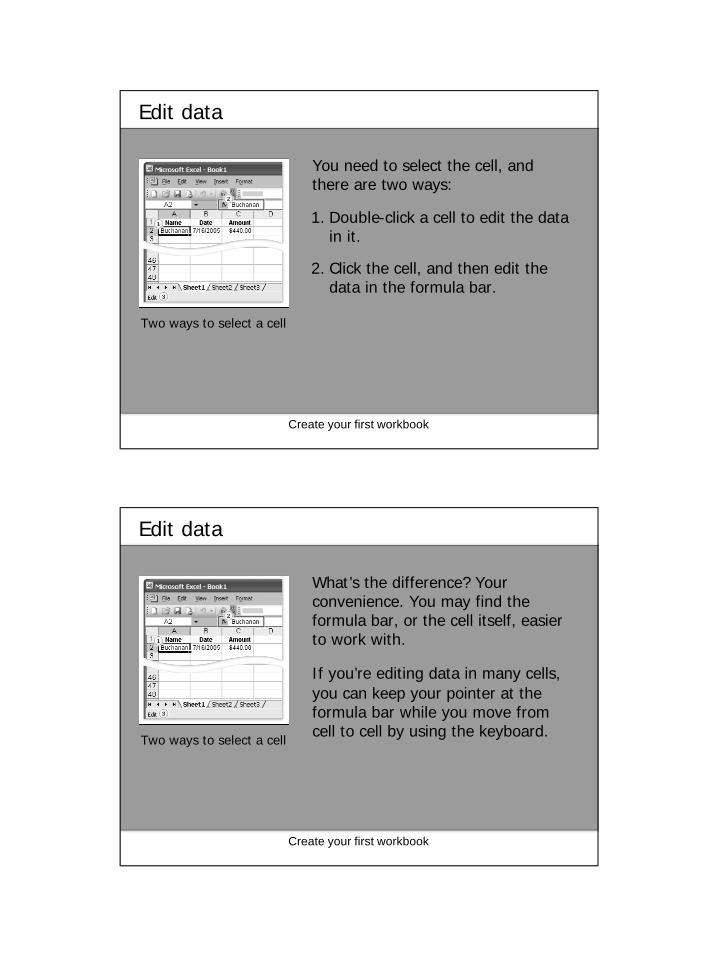
You need to select the cell, and there are two ways:
Two ways to select a cell
1. Double-click a cell to edit the data in it.
2. Click the cell, and then edit the data in the formula bar.
Create your first workbook
Edit data
What’s the difference? Your convenience. You may find the formula bar, or the cell itself, easier to work with.
Two ways to select a cell
If you’re editing data in many cells, you can keep your pointer at the formula bar while you move from cell to cell by using the keyboard.

Create your first workbook
Edit data
As the picture shows, after you select the cell:
The worksheet now says Edit in the status bar.
If you don’t see the status bar, click Status Bar on the View menu.
3. The worksheet says Edit in the lower-left corner, on the status bar.
Create your first workbook
Edit data
While the worksheet is in Edit mode, many commands are temporarily unavailable (these commands are gray on the menus).
The worksheet now says Edit in the status bar.
What can you do? Well, you can delete letters or numbers by pressing BACKSPACE, or by selecting them and then pressing DELETE.

Create your first workbook
Edit data
You can edit letters or numbers by selecting them and then typing something different.
You can insert new letters or numbers into the cell’s data by positioning the insertion point and typing them.
The worksheet now says Edit in the status bar.
Create your first workbook
Edit data
Whatever you do, when you’re all through, remember to press ENTER or TAB so that your changes stay in the cell.
The worksheet now says Edit in the status bar.

Create your first workbook
Remove data formatting
Surprise! Someone else has used your worksheet, filled in some data, and made the number in cell C6 bold and red to highlight the fact that Peacock made the highest sale.
But that customer changed her mind, so the final sale was much smaller.
Formatting stays with the cell.
Create your first workbook
Remove data formatting
You go to make the fix.
Formatting stays with the cell.
1. The original number is formatted bold and red.
2. You delete the original figure.
3. You enter a new number. Bold and red again!
What gives here?
Create your first workbook
Remove data formatting
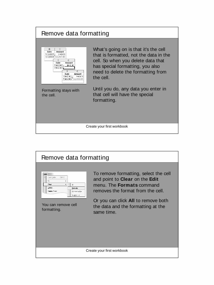
What’s going on is that it’s the cell that is formatted, not the data in the cell. So when you delete data that has special formatting, you also need to delete the formatting from the cell.
Until you do, any data you enter in that cell will have the special formatting.
Formatting stays with the cell.
Create your first workbook
Remove data formatting
To remove formatting, select the cell and point to Clear on the Editmenu. The Formats command removes the format from the cell.
Or you can click All to remove both the data and the formatting at the same time.
You can remove cell formatting.
Create your first workbook
Insert a column or a row
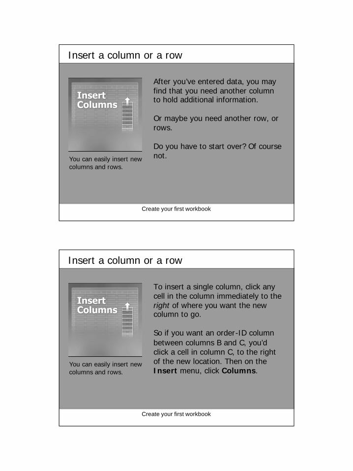
After you’ve entered data, you may find that you need another column to hold additional information.
Or maybe you need another row, or rows.
Do you have to start over? Of course not. You can easily insert new
columns and rows.
Create your first workbook
Insert a column or a row
To insert a single column, click any cell in the column immediately to the right of where you want the new column to go.
So if you want an order-ID column between columns B and C, you’d click a cell in column C, to the right of the new location. Then on the Insert menu, click Columns.
You can easily insert new columns and rows.

Create your first workbook
Insert a column or a row
To insert a single row, click any cell in the row immediately below where you want the new row to go.
For example, to insert a new row between row 4 and row 5, click a cell in row 5. Then on the Insertmenu, click Rows.
You can easily insert new columns and rows.
Create your first workbook
Insert a column or a row
Excel gives a new column or row the heading its place requires, and changes the headings of later columns and rows.
You can easily insert new columns and rows.

Create your first workbook
Suggestions for practice
1. Edit data.
2. Delete formatting from a cell.
3. Work in Edit mode.
4. Insert and delete columns and rows.
Online practice (requires Excel 2003)
Create your first workbook
Test 3, question 1
To delete the formatting from a cell, you would: (Pick one answer.)
1. Delete the cell contents.
2. Click the Format menu.
3. Click the Edit menu.

Create your first workbook
Test 3, question 1: Answer
Click the Edit menu.
Then point to Clear and click Formats.
Create your first workbook
Test 3, question 2
To add a column, click a cell in the column to the right of where you want the new column. (Pick one answer.)
1. True.
2. False.
Create your first workbook
Test 3, question 2: Answer
True.
Then on the Insert menu, click Columns to insert the column.
Create your first workbook
Test 3, question 3
To add a new row, click a cell in the row immediately above where you want the new row. (Pick one answer.)
1. True.
2. False.

Create your first workbook
Test 3, question 3: Answer
False.
To insert a new row, click a cell in the row immediately below where you want the new row. Then on the Insertmenu, click Rows.
Microsoft® Office Excel® for the Public Works Professional
Enter formulas
Course contents
• Overview: Simple calculations in Excel
• Lesson 1: Get started
• Lesson 2: Use cell references
• Lesson 3: Simplify formulas by using functions
•Each lesson includes a list of suggested tasks and a set of test questions.
• After you try Excel, you’ll never go back to a calculator. In this course you’ll learn how to add, divide, multiply, and subtract by typing formulas into Excel worksheets.
Overview: Simple calculations in Excel
• You’ll also learn how to use simple formulas that automatically update their results when values change.

Course goals
• Do math by typing simple formulas to add, divide, multiply, and subtract.
• Use cell references in formulas, so that Excel can automatically update results when values change or when you copy formulas.
• Use functions (prewritten formulas) to add up values, calculate averages, and find the smallest or largest value in a range of values.
Lesson 1
Get started

Get started
• In this lesson, you’ll learn how to use Excel as your calculator by typing simple formulas into cells.
• You’ll also learn how to total all the values in a column with a formula that updates its results if values change later on.
• We’ll start with the example worksheet shown in the picture.
A budget worksheet needs an amount in cell C6.
Begin with an equal sign
• Two CDs purchased in February cost $12.99 and $16.99. The total of these two values is the CD expense for the month.
• You do math in Excel by typing simple formulas into cells. Excel formulas always begin with an equal sign (=). Typing a formula in a
worksheet
Begin with an equal sign
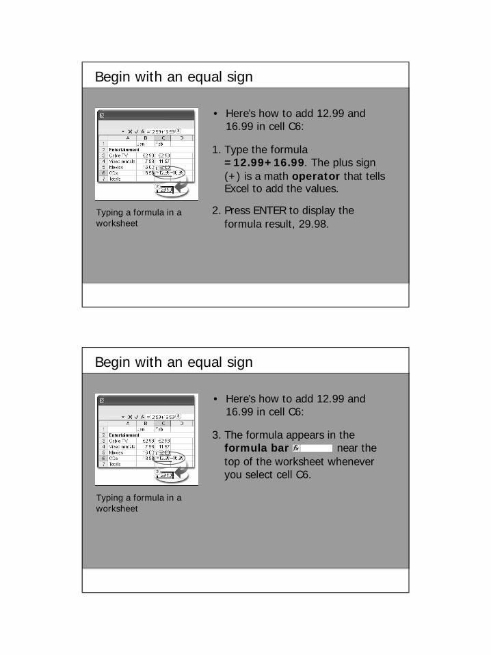
• Here’s how to add 12.99 and 16.99 in cell C6:
Typing a formula in a worksheet
1. Type the formula =12.99+16.99. The plus sign (+) is a math operator that tells Excel to add the values.
2. Press ENTER to display the formula result, 29.98.
Begin with an equal sign
• Here’s how to add 12.99 and 16.99 in cell C6:
Typing a formula in a worksheet
3. The formula appears in the formula bar near the top of the worksheet whenever you select cell C6.

Use other math operators
• To do more than add, you can use other math operators as you type formulas into worksheet cells.
• You start each formula with an equal sign and then use a minus sign (-) to subtract, an asterisk (*) to multiply, and a forward slash (/) to divide.
Excel uses familiar signs to build formulas.
Math operators
Add (+) =10+5
Subtract (-) =10-5
Multiply (*) =10*5
Divide (/) =10/5
Total all the values in a column
•To add up the total of expenses for January, as shown in the picture, you wouldn’t have to type all those values again.
•Instead, you could use a prewritten formula, called a function.
Using the AutoSumbutton to total column values

Total all the values in a column
•To get your January total:
2. A colored marquee surrounds the cells in the formula, and the formula appears in cell B7.
Using the AutoSumbutton to total column values
1. Select cell B7, and then click the AutoSum button on the Standard toolbar. The AutoSum button adds up all the values in a range of cells.
Total all the values in a column
•To get your January total:
Using the AutoSumbutton to total column values
3. Press ENTER. This displays the SUM function result 95.94 in cell B7.
4. Select cell B7 to display the formula =SUM(B3:B6) in the formula bar.
Total all the values in a column
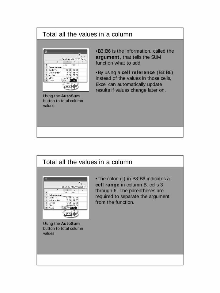
•B3:B6 is the information, called the argument, that tells the SUM function what to add.
Using the AutoSumbutton to total column values
•By using a cell reference (B3:B6) instead of the values in those cells, Excel can automatically update results if values change later on.
Total all the values in a column
•The colon (:) in B3:B6 indicates a cell range in column B, cells 3 through 6. The parentheses are required to separate the argument from the function.
Using the AutoSumbutton to total column values

Copy a formula instead of creating a new one
• Sometimes it’s easier to copy formulas than to create new ones. In this example, you’ll see how to copy the January formula and use it to add up the February expenses.
• Start by selecting cell B7, which contains the January formula. Then position the mouse pointer over the lower-right corner of the cell until the black cross (+) appears.
Copying a formula
Copy a formula instead of creating a new one
• Next:
Copying a formula
1. Drag the fill handle over cell C7 and then release it. The February total 126.93 appears in cell C7.
2. After the formula is copied, the AutoFill Options button appears to give you some formatting options.

Suggestions for practice
1. Create a formula to add.
2. Create formulas for other arithmetic.
3. Add up a column of numbers.
4. Copy a formula.
5. Add up a row of numbers.
•Online practice (requires Excel 2003)
Test 1, question 1
• What do you type into an empty cell to start a formula? (Pick one answer.)
1. *
2. (
3. =

Test 1, question 1: Answer
• =
• An equal sign tells Excel that a calculation follows it.
Test 1, question 2
• What is a function? (Pick one answer.)
1. A prewritten formula.
2. A math operator.

Test 1, question 2: Answer
• A prewritten formula.
• Functions are prewritten formulas, such as SUM, that save time.
Test 1, question 3
• A formula result is in cell C6. You wonder how you got the result. To see the formula, you do which of the following? (Pick one answer.)
1. Select cell C6, and then press CTRL+SHIFT.
2. Select cell C6, and then press F5.
3. Select cell C6.

Test 1, question 3: Answer
• Select cell C6.
• It’s that simple. The formula is visible in the formula bar near the top of the worksheet whenever you select cell C6. Or you can double-click cell C6 to see the formula in cell C6. Then press ENTER to see the formula result again in the cell.
Lesson 2
Use cell references

Use cell references
• Cell references identify individual cells or cell ranges in a worksheet. They tell Excel where to look for values to use in a formula.
• In this lesson you’ll see why Excel can automatically update the results of formulas that use cell references, and how cell references work when you copy formulas.
Cell references
Cell references Refer to values in
A10 the cell in column A and row 10
A10,A20 cell A10 and cell A20
A10:A20 the range of cells in column A and rows 10 through 20
B15:E15 the range of cells in row 15 and columns B through E
A10:E20 the range of cells in columns A through E and rows 10 through 20
Update formula results
• Suppose it turned out that the 11.97 in cell C4 for video rentals in February was incorrect. A rental of 3.99 was left out.
• To add 3.99 to 11.97, you would select cell C4 and type this formula into the cell:
Excel can automatically update totals to include changed values. • =11.97+3.99

Update formula results
• As the picture shows, when the value in cell C4 changes, Excel automatically updates the February total in cell C7 from 126.93 to 130.92.
Excel can automatically update totals to include changed values.
• Excel can do this because the original formula =SUM(C3:C6) in cell C7 contains cell references.
Update formula results
• If you had entered 11.97 and other specific values into a formula in cell C7, Excel would not be able to update the total.
Excel can automatically update totals to include changed values.
• You’d have to change 11.97 to 15.96 not only in cell C4, but in the formula in cell C7 as well.
Other ways to enter cell references
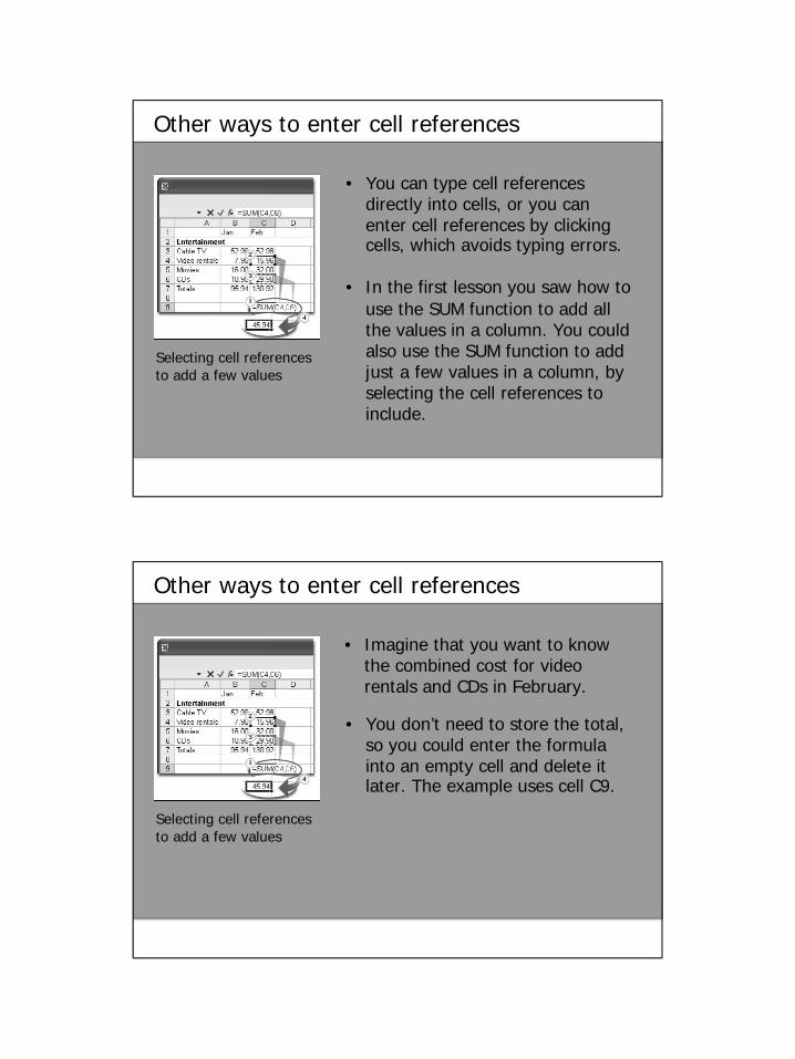
• You can type cell references directly into cells, or you can enter cell references by clicking cells, which avoids typing errors.
• In the first lesson you saw how to use the SUM function to add all the values in a column. You could also use the SUM function to add just a few values in a column, by selecting the cell references to include.
Selecting cell references to add a few values
Other ways to enter cell references
• Imagine that you want to know the combined cost for video rentals and CDs in February.
Selecting cell references to add a few values
• You don’t need to store the total, so you could enter the formula into an empty cell and delete it later. The example uses cell C9.

Other ways to enter cell references
• Here’s how to enter the formula:
Selecting cell references to add a few values
1. Type the equal sign, type SUM, and type an opening parenthesis in cell C9.
2. Click cell C4, then type a comma in cell C9.
Other ways to enter cell references
• Here’s how to enter the formula:
Selecting cell references to add a few values
3. Click cell C6. Then type a closing parenthesis in cell C9.
4. Press ENTER to display the formula result of 45.94. The arguments C4 and C6 tell the SUM function what values to calculate with.

Reference types
•Now that you’ve learned more about using cell references, it’s time to talk about the different types of references that are used in formulas: absolute, relative, and mixed.
Relative and absolute cell references
Reference types
Relative and absolute cell references
1. Relative references automatically change as they are copied down a column or across a row.
2. Absolute references are fixed; they don’t change if you copy a formula from one cell to another. Absolute references have dollar signs ($) like this: $D$9.
•Here are the details:

Reference types
Relative and absolute cell references
•A mixed cell reference has either an absolute column and a relative row, or an absolute row and a relative column.
•As a mixed reference is copied from one cell to another, the absolute reference stays the same but the relative reference changes.
Use an absolute cell reference
• Say you receive a package of entertainment coupons offering a 7 percent discount for video rentals. How much could you save in a month by using the coupons?
• To figure it out, you could create a formula to multiply those February expenses by 7 percent, using absolute references to refer to cells that you don’t want to change as the formula is copied.
Using an absolute cell reference

Use an absolute cell reference
• Type the discount rate of 0.07 in the empty cell D9, and then type a formula in cell D4, starting with =C4*. Then enter a dollar sign ($) and D to make an absolute reference to column D, and $9 to make an absolute reference to row 9.
Using an absolute cell reference • Your formula will multiply the
value in cell C4 by the value in cell D9.
Use an absolute cell reference
• Next, copy the formula from cell D4 to D5 by using the fill handle .
Using an absolute cell reference
• As the formula is copied, the relative cell reference changes from C4 to C5, while the absolute reference to the discount in D9 does not change—it remains $D$9 in each row it is copied to.

Use an absolute cell reference
• So, to recap the relative and absolute cell references in the example:
Using an absolute cell reference
1. Relative cell references change from row to row.
2. The absolute cell reference always refers to cell D9.
3. Cell D9 contains the value for the 7 percent discount.
Suggestions for practice
1. Type cell references in a formula.
2. Select cell references in a formula.
3. Use an absolute reference in a formula.
4. Add up several results.
5. Change values and totals.
•Online practice (requires Excel 2003)

Test 2, question 1
• What is an absolute cell reference? (Pick one answer.)
1. The cell reference automatically changes when the formula is copied down a column or across a row.
2. The cell reference is fixed.
3. The cell reference uses the A1 reference style.
Test 2, question 1: Answer
• The cell reference is fixed.
• Absolute cell references won’t change if you copy a formula from one cell to another.
Test 2, question 2
• Which cell reference refers to a range of cells in column B, rows 3 through 6? (Pick one answer.)
1. (B3:B6)
2. (B3,B6)
Test 2, question 2: Answer
• (B3:B6)
• The colon indicates a range of cells starting at B3 and including B4, B5, and B6.

Test 2, question 3
• If you copy the formula =C4*$D$9 from cell C4 to cell C5, what will the formula be in cell C5? (Pick one answer.)
1. =C5*$D$9
2. =C4*$D$
3. =C5*$E$10
Test 2, question 3: Answer
• =C5*$D$9
• As the formula is copied, the relative cell reference, C4, changes to C5. The absolute cell reference, $D$9, does not change; it remains the same in each row it is copied to.

Lesson 3
Simplify formulas by using functions
Simplify formulas by using functions
• SUM is just one of the many Excel functions. These prewritten formulas simplify the process of entering calculations, making it easy and quick to create formulas that might be difficult to build for yourself.
• In this lesson you’ll see how to speed up tasks with a few easy functions.
Function names express long formulas quickly.
Function Calculates
AVERAGE an average
MAX the largest number
MIN the smallest number
Find an average
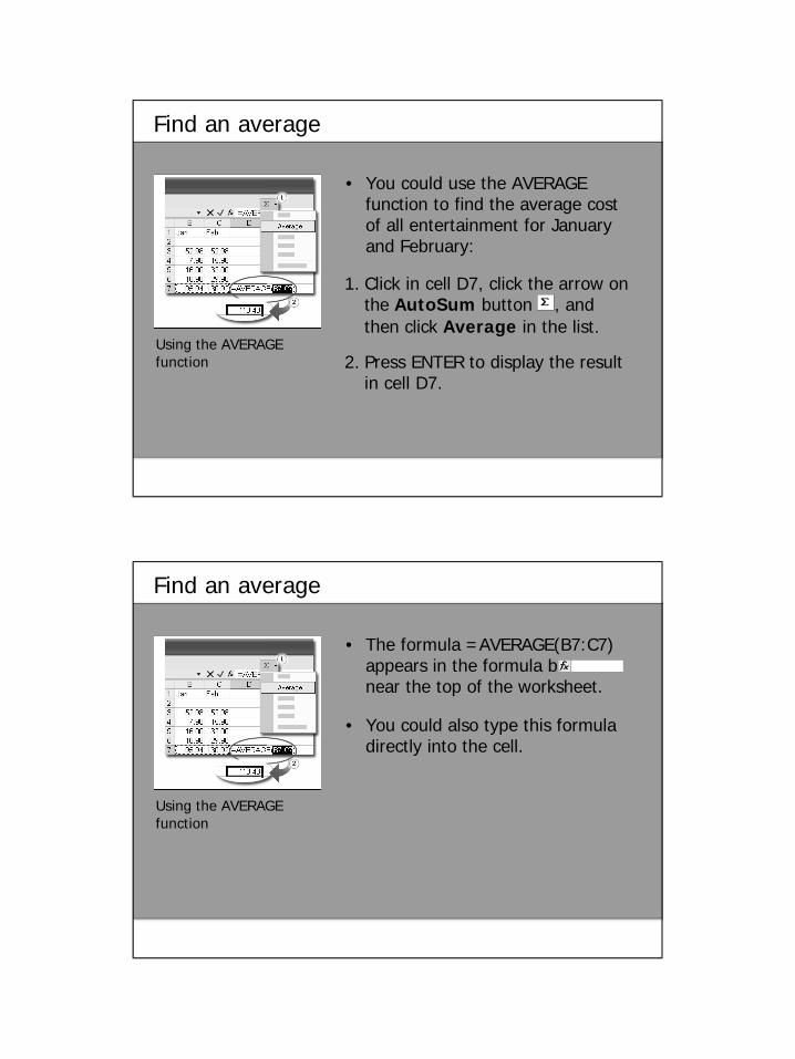
• You could use the AVERAGE function to find the average cost of all entertainment for January and February:
Using the AVERAGE function
1. Click in cell D7, click the arrow on the AutoSum button , and then click Average in the list.
2. Press ENTER to display the result in cell D7.
Find an average
• The formula =AVERAGE(B7:C7) appears in the formula bar near the top of the worksheet.
Using the AVERAGE function
• You could also type this formula directly into the cell.

Find the largest or smallest value
• The MAX function finds the largest number in a range of numbers, and the MIN function finds the smallest number in a range.
Using the MAX function
Find the largest or smallest value
• Here’s a formula to find the largest value in the set:
Using the MAX function
1. Click in cell F7, click the arrow on the AutoSum button, and then click Max in the list.
2. Press ENTER to display the result in F7.
• The largest value is 131.95.

Find the largest or smallest value
• Finding the smallest value in the range is a similar process: You’d click Min in the list and press ENTER.
Using the MAX function
• The smallest value would be 131.75.
Print formulas
•You can print formulas to put up on your bulletin board to remind you how to create them.
Formulas displayed on the worksheet
1. On the Tools menu, point to Formula Auditing, and then click Formula Auditing Mode .
2. Print as you usually would.
What’s that funny thing in my worksheet?
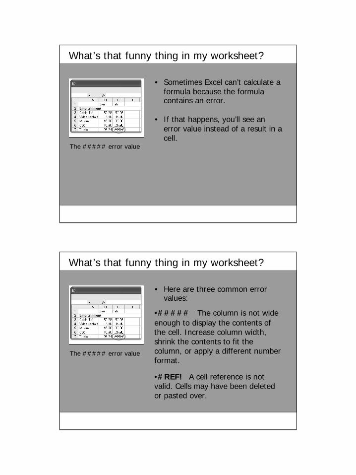
• Sometimes Excel can’t calculate a formula because the formula contains an error.
• If that happens, you’ll see an error value instead of a result in a cell.
The ##### error value
What’s that funny thing in my worksheet?
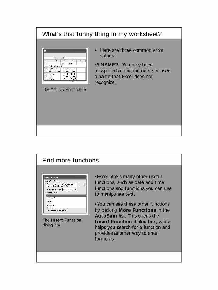
• Here are three common error values:
The ##### error value
•##### The column is not wide enough to display the contents of the cell. Increase column width, shrink the contents to fit the column, or apply a different number format.
•#REF! A cell reference is not valid. Cells may have been deleted or pasted over.
What’s that funny thing in my worksheet?
• Here are three common error values:
The ##### error value
•#NAME? You may have misspelled a function name or used a name that Excel does not recognize.
Find more functions
•Excel offers many other useful functions, such as date and time functions and functions you can use to manipulate text.
•You can see these other functions by clicking More Functions in the AutoSum list. This opens the Insert Function dialog box, which helps you search for a function and provides another way to enter formulas.
The Insert Functiondialog box

Find more functions
•When the dialog box is open, you can type what you want to do in the Search for a function box, or select a category and then scroll through the list of functions.
The Insert Functiondialog box
Suggestions for practice
1. Find an average.
2. Find the largest number.
3. Find the smallest number.
4. Display and hide formulas.
5. Create and fix error values.
6. Create and fix the error value #NAME.
•Online practice (requires Excel 2003)

Test 3, question 1
• How would you print formulas? (Pick one answer.)
1. Click Print on the File menu.
2. Click Normal on the View menu, and then click Print.
3. Point to Formula Auditing on the Tools menu, click Formula Auditing Mode , and then print as usual.
Test 3, question 1: Answer
• Point to Formula Auditing on the Tools menu, click Formula Auditing Mode, and then print as usual.
• This displays the formulas on your worksheet before you print.
Test 3, question 2
• What does ##### mean? (Pick one answer.)
1. The column isn’t wide enough to display the content.
2. The cell reference isn’t valid.
3. You’ve misspelled a function name or used a name that Excel doesn’t recognize.
Test 3, question 2: Answer
• The column isn’t wide enough to display the content.
• You can increase the column width to display the content.

Microsoft® Office Excel® for the Public Works Professional
How to create a chart
Course contents
• Overview: Telling the story behind the data
• Lesson 1: Create a basic chart
• Lesson 2: Tell the wizard what you want
•Each lesson includes a list of suggested tasks and a set of test questions.

• A chart gets your point across—fast. With a chart, you turn worksheet data into a picture, where you can make a comparison or a trend visible at a glance.
Overview: Telling the story behind the data
• This course takes you through the basics of how to create charts in Excel.
Course goals
• Create a chart using the Chart Wizard.
• Make selections in the Chart Wizard.
• Understand basic chart terminology.

Lesson 1
Create a basic chart
Create a basic chart
• This lesson covers how to make a quick and basic no-frills chart in about ten seconds.
• Then you'll see how the text and numbers from a worksheet become the contents of a chart, and you'll learn a few other chart basics before the practice session at the end of the lesson.
Charts transform data into pictures.

Meet the wizard
• Suppose you're looking at a worksheet that shows how many cases of Sir Rodney's Marmalade were sold by each of three salespeople in each of three months.
• How would you create a chart to show how the salespeople compare against each other every month?
The Chart Wizard
2. Click the Chart Wizard button on the toolbar to open the Chart Wizard.
Meet the wizard
The Chart Wizard
1. Select the data that you want to chart, as well as the column and row labels.
3. When the wizard opens, the Column chart type is selected by default.
4. Click the Finish button at the bottom of the wizard.

How worksheet data appears in the chart
• Each row of salesperson data has been given a color in this chart.
• The chart legend, which was created from the row titles in the worksheet, tells which color represents the data for each salesperson.
Worksheet row data is transformed into columns.
How worksheet data appears in the chart
• Each chart column reaches a height proportional to the value in the cell that it represents. You can see at once how the salespeople stack up against each other as well as month by month.
• On the left side of the chart, Excel has created a scale of numbers by which you can interpret the column heights.
Worksheet row data is transformed into columns.

Update and place charts
•The wizard placed this chart as an object on the worksheet along with the data, as shown in the picture.
•When a chart is an object, it can be moved and resized. It can also be printed right along with the source data.
A chart on the same worksheet as the data
Suggestions for practice
1. Create a chart.
2. Update chart data.
3. Move a chart.
4. Resize a chart.
5. Look at other chart types.
6. Delete a chart.
•Online practice (requires Excel 2003)

Test 1, question 1
• What is the most important thing about a chart? (Pick one answer.)
1. That it makes your point clearly.
2. That it has a lot of colors.
3. That it's the most sophisticated chart type.
Test 1, question 1: Answer
• That it makes your point clearly.
• Making a chart that doesn't get your point across is, well, pointless.

Test 1, question 2
• A chart placed on the worksheet can be printed along with the worksheet data. (Pick one answer.)
1. True.
2. False.
Test 1, question 2: Answer
• True.
• It can also be moved and resized.

Test 1, question 3
• What must you do to refresh a chart when you revise the worksheet data it displays? (Pick one answer.)
1. Press SHIFT+CTRL.
2. Nothing.
3. Press F6.
Test 1, question 3: Answer
• Nothing.
• When you revise a value in the worksheet, the chart is automatically refreshed. Just sit back and relax.

Test 1, question 4
• A chart legend provides the data that appears in row or column titles. (Pick one answer.)
1. True.
2. False.
Test 1, question 4: Answer
• False.
• The row or column titles provide the text for the legend, showing which chart colors signify which row or column.

Lesson 2
Tell the wizard what you want
Tell the wizard what you want
• In this lesson you'll learn about an important choice that you can make in the Chart Wizard.
• You choose whether your chart compares salespeople to each other, month after month—or whether it compares months to each other, salesperson by salesperson.
• The picture shows both ways.
Choose how the Chart Wizard compares your data.
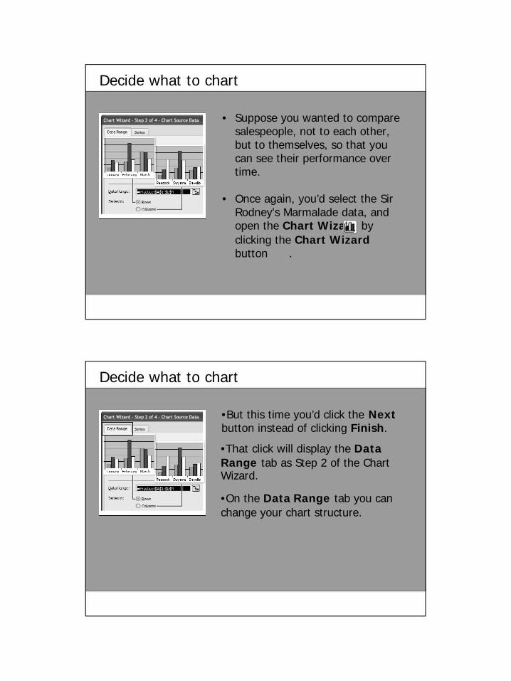
• Suppose you wanted to compare salespeople, not to each other, but to themselves, so that you can see their performance over time.
• Once again, you’d select the Sir Rodney's Marmalade data, and open the Chart Wizard by clicking the Chart Wizardbutton .
Decide what to chart
Decide what to chart
•But this time you’d click the Nextbutton instead of clicking Finish.
•That click will display the Data Range tab as Step 2 of the Chart Wizard.
•On the Data Range tab you can change your chart structure.
Decide what to chart
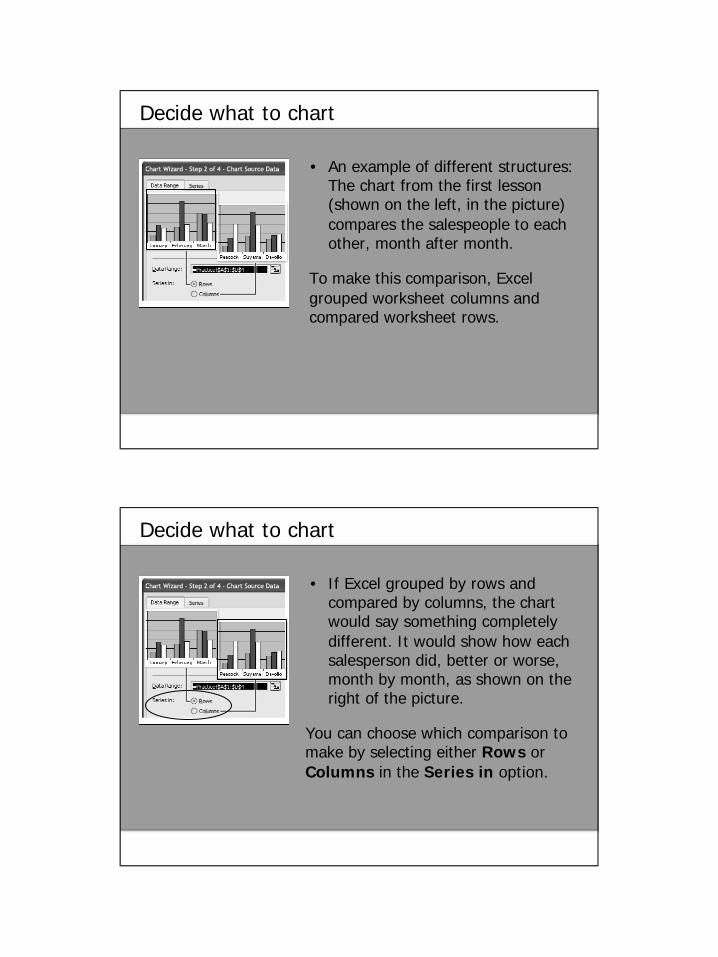
• An example of different structures: The chart from the first lesson (shown on the left, in the picture) compares the salespeople to each other, month after month.
To make this comparison, Excel grouped worksheet columns and compared worksheet rows.
Decide what to chart
• If Excel grouped by rows and compared by columns, the chart would say something completely different. It would show how each salesperson did, better or worse, month by month, as shown on the right of the picture.
You can choose which comparison to make by selecting either Rows or Columns in the Series in option.

Decide what to chart
• On the Series tab, you can delete or add a data series for the chart. For example, you might decide to chart only two of the salespeople instead of all three.
Add titles
• It's a good idea to add descriptive titles to your chart so that readers don't have to guess what the chart's about.
• You can add a title for the chart by typing in the Chart title box, for example: Sir Rodney's Marmalade.Enter chart and axis
titles in the Chart Wizard.

Add titles
• Next is a title box for the Category (X) axis. This is Excel's term for the categories at the bottom of the chart (January and so on).
Enter chart and axis titles in the Chart Wizard.
• You could call this axis First Quarter Sales.
Add titles
• Next is a title box for the Value (Y) axis. In this chart, it's the scale of numbers that show how many cases the salespeople sold.
Enter chart and axis titles in the Chart Wizard.
• You could call this axis Cases Sold.

Even more tabs and options
•There are more tabs in the Chart Wizard. Each tab includes a preview so that you can see what your chart looks like if you change any of your choices. Various chart types offer different sets of options.
1. Gridlines
2. Legend
3. Data table
Even more tabs and options
•For a clustered column chart, the tabs are:
• Axes
• Gridlines
• Legends
• Data Labels
• Data Table
• Chart Location
1. Gridlines
2. Legend
3. Data table

Suggestions for practice
1. Change a chart by changing what's charted:
• Change the values (the data series) that are charted.
2. Explore options in the wizard:
• Titles, axes, and data labels; gridlines; legend; data labels again; data table.
3. Make a pie chart.
•Online practice (requires Excel 2003)
Test 2, question 1
• What is a data series? (Pick one answer.)
1. It's the values that are charted.
2. It's the headings under which the values are organized.
3. It's the key that shows what the values on the chart are.

Test 2, question 1: Answer
• It's the values that are charted.
• You choose what your chart says by charting the values from either the rows or the columns of the worksheet.
Test 2, question 2
• Which of these can you do on the Data Range tab in the Chart Wizard? (Pick one answer.)
1. Delete a data series.
2. Change the data series that is charted.
3. Label a data series.
Test 2, question 2: Answer
• Change the data series that is charted.
• This is where you can change what your chart says.
Test 2, question 3
• The Category (X) axis is the scale of numbers on the chart. (Pick one answer.)
1. True.
2. False.

Test 2, question 3: Answer
• False.
• It's the Value (Y) axis that shows the scale of numbers to indicate the magnitude of values.
Microsoft® Office Excel® for the Public Works Professional
How to use lists

Course contents
• Overview: Lists in Excel 2003
• Lesson 1: Create a list
• Lesson 2: Sort and filter a list
•Each lesson includes a list of suggested tasks and a set of test questions.
Overview: Lists in Excel 2003
• There’s a new List command in Excel 2003 that makes it easy to create orderly rows of data such as addresses, names of clients or products, and quarterly sales amounts.
• The new List command also makes it easy to total up values and to sort and filter data.

Course goals
• Create a list using the List command.
• Add up values in lists using the List toolbar.
• Use the AutoFilter arrows to sort and filter list data.
Lesson 1
Create a list

Create a list
• Using the new List command to enter list data has several benefits.
• For example, AutoFilter arrows are applied automatically in a convenient way (more on that in Lesson 2).
The new List command is on the Data menu.
• Also, you can use the new Toggle Total Row button to total the last column in the list.
Use the List command
• Imagine that you've already entered some data for salespeople into Excel.
• To have Excel see this data as a list, click any cell within the data, and then:
Creating a list 1. Point to List on the Data menu.
2. Click Create List.
• (Continued on next slide.)

Creating a list
• The Create List dialog box appears.
• You confirm that your data has headers (column headings), and that the indicated data is what you want included in the list.
• Then the data becomes a list.
Use the List command, cont’d.
Now you have a list
• Now that the data is a list:
1. AutoFilter arrows are automatically added in the header row.
2. A dark blue border appears around the list.
• (Continued on next slide.)

Now you have a list, cont’d.
• The dark blue border indicates the range of cells in your list.
• You can have more than one list on a worksheet when you use the List command.
• The blue border distinguishes one list from another and helps you to tell list data from other worksheet data.
Add a row or a column to the list
• The row that contains an asterisk at the bottom is the insert row—the row you use to insert additional data.
List with an insert row
• (Continued on next slide.)
• As soon as you enter data to the insert row, another empty insert row is added to the list, so that you can continue to add data.
Add a row or a column to the list, cont’d.
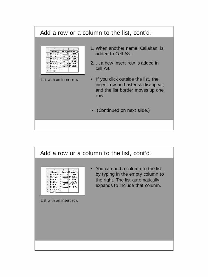
List with an insert row • If you click outside the list, the insert row and asterisk disappear, and the list border moves up one row.
• (Continued on next slide.)
1. When another name, Callahan, is added to Cell A8…
2. … a new insert row is added in cell A9.
Add a row or a column to the list, cont’d.
List with an insert row
• You can add a column to the list by typing in the empty column to the right. The list automatically expands to include that column.

Add up values
•The Toggle Total Row button on the new List toolbar totals the last column in the list.
•To get a total in column C of the example:
1. Click the Toggle Total Rowbutton on the List toolbar...
2. ... to add a Total row to the list.
The Toggle Total Rowbutton on the new Listtoolbar
Suggestions for practice
1. Create a list.
2. Add a total to a list.
3. Add a row and a column.
•Online practice (requires Excel 2003)

Test 1, question 1
• On which menu is the List command? (Pick one answer.)
1. On the Tools menu.
2. On the Data menu.
3. On the List menu.
Test 1, question 1: Answer
• On the Data menu.
• On the Data menu in Excel 2003, point to List, and then click Create List.

Test 1, question 2
• How do you add a column to a list? (Pick one answer.)
1. Type in the empty column to the right.
2. On the Data menu, point to List, and then click Resize List.
3. Right-click the empty column to the right, click Insert, and then click Entire Column.
Test 1, question 2: Answer
• Type in the empty column to the right.
• The list will automatically expand to include that column.

Lesson 2
Sort and filter a list
Sort and filter a list
• When you create a list with the List command, you automatically add AutoFilter arrows to the list.
• You can use the AutoFilter arrows for sorting and filtering your list data.
• The List command also lets you work with several lists on a single worksheet.
AutoFilter arrows
How to sort
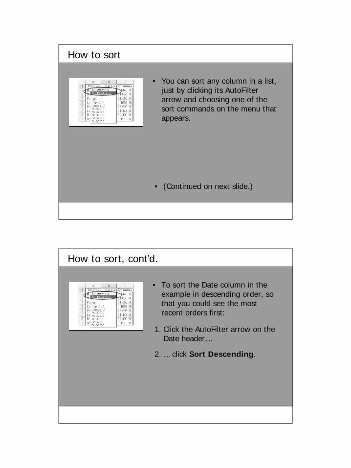
• You can sort any column in a list, just by clicking its AutoFilter arrow and choosing one of the sort commands on the menu that appears.
• (Continued on next slide.)
How to sort, cont’d.
• To sort the Date column in the example in descending order, so that you could see the most recent orders first:
1. Click the AutoFilter arrow on the Date header…
2. … click Sort Descending.

How to filter
• Filtering list data is as simple as sorting. Excel will automatically show only the data you specify.
• To see only sales made by Peacock, instead of everyone’s sales:
1. Click the AutoFilter arrow on the Name column.
2. Select Peacock.
More than one list on a worksheet
•When you use the List command, you can have more than one list on a worksheet.
•You can add or delete a row in one list without adding or deleting a row in a list next to it, an ability new in Excel 2003.
You can add a row to the list on the right without adding a row to the list on the left.
•You can also sort those lists separately, because using the Listcommand automatically gives each list its own AutoFilter arrows.

Suggestions for practice
1. Sort a list
2. Filter a list.
•Online practice (requires Excel 2003)
Test 2, question 1
• How do you sort list data in descending order? (Pick one answer.)
1. Click Sort on an AutoFilter arrow in the list.
2. Click Sort Descending on an AutoFilter arrow in the list.
3. Click Sort Descending on the List toolbar.

Test 2, question 1: Answer
• Click Sort Descending on an AutoFilter arrow in the list.
Test 2, question 2
• You can have more than one list on a worksheet, and you can add or delete a row in one list without adding or deleting a row in the list next to it . (Pick one answer.)
1. True.
2. False.

Test 2, question 2: Answer
• True.
Microsoft® Office Excel® for the Public Works Professional
Statistical functions in Excel

Course contents
• Overview: Using statistical functions, formulas
• Lesson 1: Excel and statistics—The basics
• Lesson 2: Write good formulas
• Lesson 3: Which function to use?
•Each lesson includes a list of suggested tasks and a set of test questions.
Overview: Using statistical functions, formulas
• Learn about using statistical functions and formulas in Microsoft Office Excel 2003, from the very basics to choosing the right function for you.
Learn also how to troubleshoot common problems.

Course goals
• Use a statistical function in an Excel spreadsheet.
• Assess which statistical function to use in a particular situation.
• Avoid some common errors when using functions.
• Understand why some statistical formula results are more accurate in Excel 2003 than in previous versions.
Lesson 1
Excel and statistics: The basics

Excel and statistics: The basics
• Building a formula in Excel using statistical functions is no more difficult than using any other function.
• You just have to know how to use Excel functions and know a bit about statistics.
Use Excel to manage your statistical data.
Excel and statistics: The basics
• Using Excel to do everyday statistical calculations can save you a lot of time and effort.
Use Excel to manage your statistical data.
• This lesson will explain the basics of why you might want to use Excel, and gives a quick reminder on how to build formulas in Excel.

Why Excel?
• There are many practical applications of statistics in Excel:
Excel statistical functions have many uses.
• A sales manager might want to project the next quarter's sales (TREND function)
• A teacher might want to grade on a curve based on average scores (AVERAGE, MEDIAN, or even MODE functions)
Why Excel?
• A manufacturer checking product quality might be interested in the range of items that fall out of acceptable quality limits (STDEV or VAR functions)
Excel statistical functions have many uses.
• A market researcher might need to find out how many responses in a survey fell within a range of responses (FREQUENCY function)

Variance in action
• Imagine a sales manager looking at the sales figures for three different salespeople to compare their performances.
• One of the many statistical functions the manager could use is variance (VAR).
Variance in action
• Variance measures how different the individual values of the data are from one another.
• Data with low variance contains values that are identical or similar, such as 6, 7, 6, 6, 7.
• Data with high variance contains values that are not similar, such as 598, 1, 134, 5, 92.

How to construct a statistical formula
•If you know how to use a function in Excel, you can use a statistics function.
•They are written in the same way:
1. Always start with an equal sign (=).
2. Then the function name.
3. Then the arguments in parentheses.
Finding the variance based on a range
When Excel isn't enough
• If you're doing heavy-duty statistical analysis, Excel might not be powerful enough for your needs.
• An example is doing research in a lab. If you do regression analysis, Excel requires that the x values be in a single block (adjacent rows or columns), which might not be convenient for you.

When Excel isn't enough
• In these circumstances, you might want to use a dedicated statistical package because it covers a larger set of statistical analysis options and related functions.
• Some packages also display additional outputs associated with a particular analysis.
When Excel isn't enough
• Many of these statistical analysis programs are commercially available.
• There are also specially designed add-ins for Excel from other companies.
• Some of them can be found in the Office Marketplace on Microsoft Office Online.

Suggestions for practice
1. Calculate variance by typing cell references.
2. Calculate variance by clicking the cell references.
3. Calculate variance by dragging across a cell range.
4. Interpret the results.
•Online practice (requires Excel 2003)
Test 1, question 1
• To use statistical functions with Excel, you must have: (Pick one answer.)
1. A statistical add-in package.
2. You can't do statistics in Excel.
3. A computer with Excel installed.
4. A degree in statistics.

Test 1, question 1: Answer
• A computer with Excel installed.
• All you need is Excel; it has many statistical functions built in.
Test 1, question 2
• How do you create a statistical formula in Excel? (Pick one answer.)
1. It's exactly like any other formula: type the equal sign (=) and then the function name followed by the data information.
2. On the Data menu, click Statistics.
3. On the Insert menu, click Statistics Function.

Test 1, question 2: Answer
• It's exactly like any other formula: type the equal sign (=) and then the function name followed by the data information.
• Statistical formulas are no more complicated than any other formula.
Test 1, question 3
• Which of these is a formula in Excel? (Pick one answer.)
1. STDEV
2. =STDEV(A1:A33)
3. NaCl

Test 1, question 3: Answer
• =STDEV(A1:A33)
• A formula in Excel includes an equal sign, a function name, and the arguments in parentheses.
Lesson 2
Write good formulas

Write good formulas
• If Excel is so great for doing statistics, why doesn't everyone use it?
Success with Excel requires good formulas.
• Sometimes it's hard to know what Excel can do.
• People can get errors when trying to get the results they want.
What's the problem?
• To build better formulas in Excel:
• Increase your knowledge of functions
• Avoid the common mistakes that many people make
Incorrectly written formulas return error messages.

What's the problem?
• Anyone using Excel — not just those using statistical functions —encounters these problems.
The main thing is to use the right function and to know how to write a proper formula.
Using an incorrectly written formula —or the wrong function — usually results in an incorrect answer.
Incorrectly written formulas return error messages.
How to solve the problem
• There are plenty of sources of information to help you out.
• You can learn to write better formulas with such resources as:
The Insert Function dialog box
• This training course
• Excel Help topics
• The Insert Function dialog box

How to solve the problem
• In the Insert Function dialog box, you can:
• Choose which type of function you're looking for
• Select a specific function from a list of functions
• Get a description of that function as well as request help on it
The Insert Function dialog box
How to solve the problem
• To open the Insert Functiondialog box, click Function on the Insert menu. Then:
1. Pick the function type you need.
2. Find the function name in the list.
3. Check the function description to make sure you've selected the right one.
4. Click the Help link if you need more information.
The Insert Function dialog box
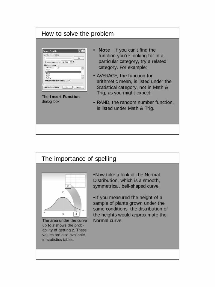
How to solve the problem
• Note If you can't find the function you're looking for in a particular category, try a related category. For example:
• AVERAGE, the function for arithmetic mean, is listed under the Statistical category, not in Math & Trig, as you might expect.
• RAND, the random number function, is listed under Math & Trig.
The Insert Function dialog box
The importance of spelling
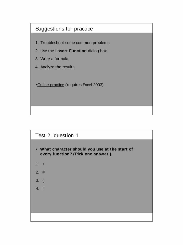
•Now take a look at the Normal Distribution, which is a smooth, symmetrical, bell-shaped curve.
•If you measured the height of a sample of plants grown under the same conditions, the distribution of the heights would approximate the Normal curve.The area under the curve
up to z shows the prob-ability of getting z. These values are also available in statistics tables.

The importance of spelling
•There are two functions in Excel for the Normal Distribution:
• NORMDIST
• NORMSDIST
The area under the curve up to z shows the prob-ability of getting z. These values are also available in statistics tables.
The importance of spelling
•In the practice session you'll use the NORMSDIST function, which calculates probabilities associated with the Standard Normal Distribution. The Standard Normal Distribution curve is centered at 0 (the mean).
The area under the curve up to z shows the prob-ability of getting z. These values are also available in statistics tables.

More common problems
• Some of the most common mistakes when building formulas include:• Forgetting the equal sign (=) at
the start of the formula.
• Inserting a space before the equal sign.
• Having your data in the wrong format (for example, as text rather than as numbers).
• Selecting the wrong data range.
Some common errors in spreadsheets
More common problems
• If you have something wrong in a formula, Excel might return an incorrect result, such as #VALUE!, as shown in the illustration on the left.
Some common errors in spreadsheets
These problems can be easily avoided. A full list of error types and ways to solve them is available in the Help topics.
Suggestions for practice
1. Troubleshoot some common problems.
2. Use the Insert Function dialog box.
3. Write a formula.
4. Analyze the results.
•Online practice (requires Excel 2003)
Test 2, question 1
• What character should you use at the start of every function? (Pick one answer.)
1. +
2. #
3. (
4. =

Test 2, question 1: Answer
• =
• Every formula must start with an equal sign.
Test 2, question 2
• Which of these is a valid formula in Excel? (Pick one answer.)
1. NORMSDIST(0.3)
2. =NORMSDIST (0.3)
3. =NORMSDIST(0.3)
4. =NORMSIDST(0.3)

Test 2, question 2: Answer
• =NORMSDIST(0.3)
This is a perfectly valid formula.
Test 2, question 3
• How do you display the Insert Function dialog box? (Pick one answer.)
1. On the Insert menu, click Function.
2. On the Function menu, click Insert.
3. On the Tools menu, click Insert Function.

Test 2, question 3: Answer
• On the Insert menu, click Function.
Lesson 3
Which function to use?

Which function to use?
• You've mastered writing formulas in Excel. You know to start with the equal sign and how to troubleshoot some error messages.
• What else could possibly cause a problem? Could you still get incorrect results?
Still have the wrong answer?
• If you're not sure which function to use, there's only so much help that Excel can give you. You need to be able to analyze your data: even when you think you know which statistical function you want, some statistical knowledge is necessary.
The Insert Functiondialog box

Still have the wrong answer?
• Many similarly named functions in Excel are related to one another.
• If you've picked a function that does something slightly different from what you intended, make sure you've got the right one.
• Check the purpose of each individual function in the Insert Function dialog box and use the link to the Help topics.
The Insert Functiondialog box
Which function?
• Another example of a statistical function that has more than one option to choose from in Excel is standard deviation.
A sample population and an entire population

Which function?
• The standard-deviation functions available in Excel are:
A sample population and an entire population
• STDEV
• STDEVA
• STDEVP
• STDEVPA
Which function?
• STDEVP and STDEVPA both use entire populations, whereas STDEV and STDEVA work on samples of populations. This is a statistical difference.
Function Type of statistical data
Type of Excel data
STDEV Sample Numeric
STDEVA Sample Numeric, logical, and text
STDEVP Population Numeric
STDEVPA Population Numeric, logical, and text

Which function?
• STDEVA and STDEVPA will recognize TRUE and FALSE text (or logical values) as well as numerals.
• STDEV and STDEVP will only recognize numeric values.
Function Type of statistical data
Type of Excel data
STDEV Sample Numeric
STDEVA Sample Numeric, logical, and text
STDEVP Population Numeric
STDEVPA Population Numeric, logical, and text
Better results in Excel 2003
•Some functions will give different results in Excel 2003 compared to previous versions of Excel:
• Various functions were improved “behind the scenes.”
• Excel 2003 uses a “two–pass”procedure, which increases the accuracy of the results.
Excel 2003 is more accurate than Excel 2002.

Suggestions for practice
1. Work with functions that accept logical values.
2. Compare values between entire population functions and sample population functions.
•Online practice (requires Excel 2003)
Test 3, question 1
• You have worked out a function in Excel, but double-checking on a calculator gives a completely different result. What should you do? (Pick one answer.)
1. Check that you've used the right Excel function.
2. Panic.
3. Find another calculator.
4. Assume Excel is correct.

Test 3, question 1: Answer
• Check that you've used the right Excel function.
• You can easily get different results by using similar, related functions. The first thing to do is check that you have the right function. It's also possible that Excel and a calculator will yield slightly different results if you're looking at a large number of significant figures.
Test 3, question 2
• If you're not sure about which function to use, what should you do? (Pick one answer.)
1. Consult a statistics text book.
2. Try them all and see what looks right.
3. Check the Insert Function dialog box.

Test 3, question 2: Answer
• Check the Insert Function dialog box.
• Use either the description in the Insert Function dialog box or the link to the Help topics to get information about what each function does.
Test 3, question 3
• You have a worksheet created in Excel 2002. When you update the worksheet in Excel 2003, some of the results change. Which result set is the most accurate? (Pick one answer.)
1. Excel 2003.
2. Excel 2002.

Test 3, question 3: Answer
• Excel 2003.
• Some functions were updated in Excel 2003 to give more accurate results.
Microsoft® Office Excel® for the Public Works Professional
Great Excel features
Course contents
• Overview: Five great features
– Lesson 1: Freeze!
– Lesson 2: Compare side by side
– Lesson 3: Sum it up, and more
– Lesson 4: Type less, get more
– Lesson 5: Call attention to the good or the bad
• Each lesson includes a list of suggested tasks and a set of test questions.
• Isn't it great when something is easier than you thought? Like keeping titles in view when scrolling down a worksheet, or adding up numbers just by selecting them?
Overview: Five great features
• In this course you’ll learn about five great Microsoft® Office Excel®2003 features that will help you to work faster and easier.

Course goals
• Freeze the upper and left panes to keep column or row titles in view while you scroll through data.
• Compare two workbooks at the same time by using the new Compare Side by Side feature in Microsoft Office Excel 2003.
• Add up numbers just by selecting them.
• Use the fill handle instead of typing to complete repetitive series of numbers, dates, or text.
• Make formatting changes automatically when values are at a certain point by using conditional formatting.
Lesson 1
Freeze!
Freeze!
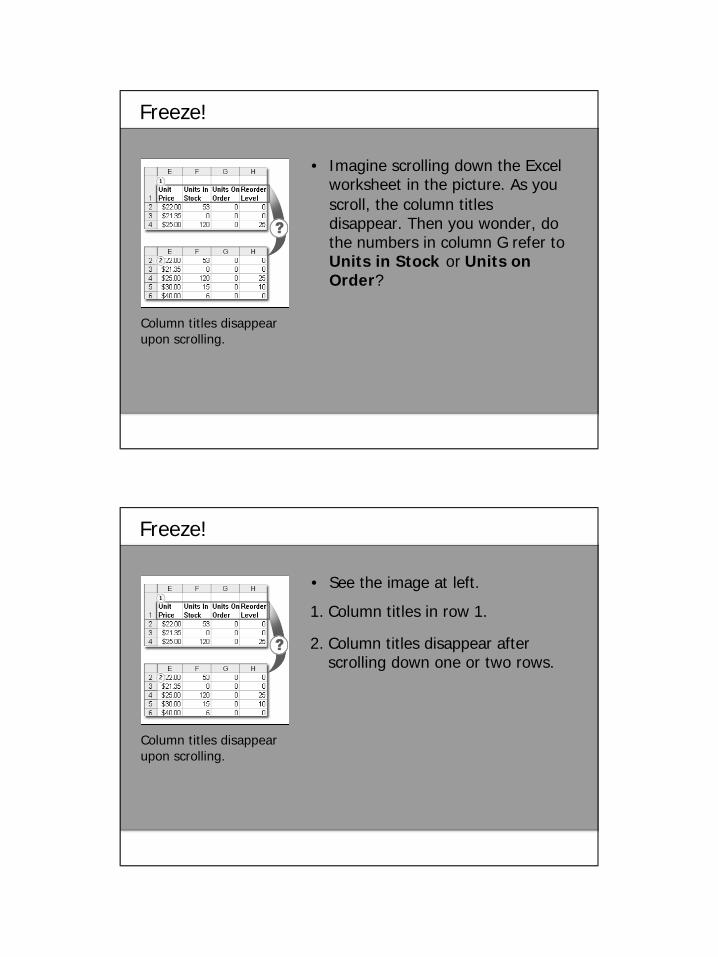
• Imagine scrolling down the Excel worksheet in the picture. As you scroll, the column titles disappear. Then you wonder, do the numbers in column G refer to Units in Stock or Units on Order?
Column titles disappear upon scrolling.
Freeze!
• See the image at left.
Column titles disappear upon scrolling.
1. Column titles in row 1.
2. Column titles disappear after scrolling down one or two rows.
Divide and conquer
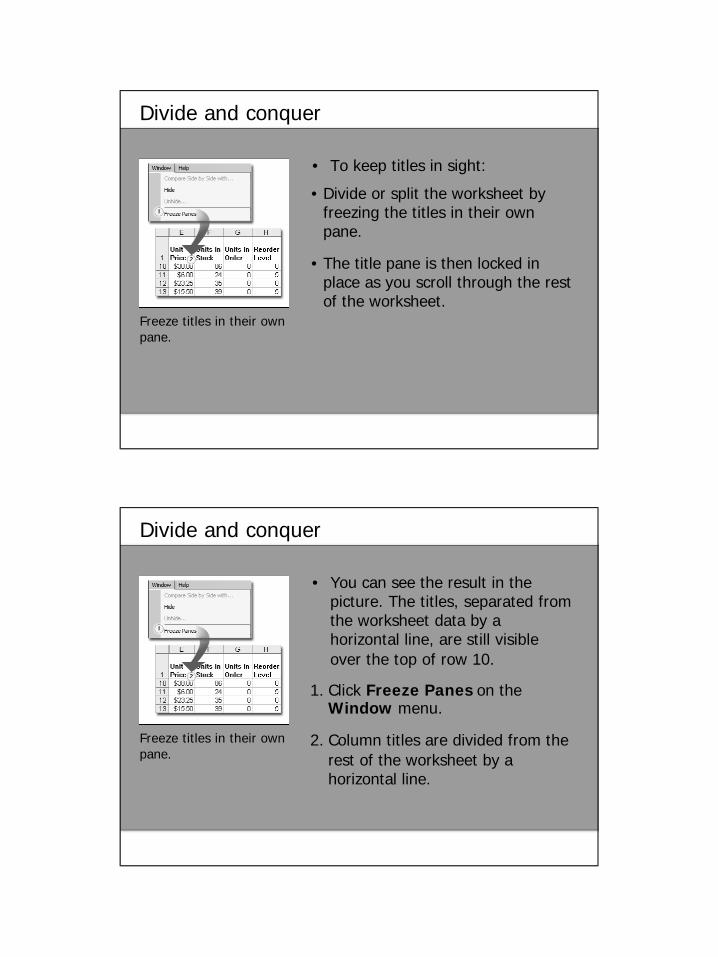
• To keep titles in sight:
Freeze titles in their own pane.
• Divide or split the worksheet by freezing the titles in their own pane.
• The title pane is then locked in place as you scroll through the rest of the worksheet.
Divide and conquer
• You can see the result in the picture. The titles, separated from the worksheet data by a horizontal line, are still visible over the top of row 10.
Freeze titles in their own pane.
1. Click Freeze Panes on the Window menu.
2. Column titles are divided from the rest of the worksheet by a horizontal line.

Freeze here
• It's not just column titles that you can freeze in place. You can also freeze row titles, or you can freeze both at the same time to keep both column and row titles.
Do not select titles to freeze panes
Freeze here
• To freeze:
1. Column titles, select the first row below the titles.
2. Row titles, select the first column to the right (for example, to keep supplier names in sight as you scroll across the worksheet).
3. Both column and row titles, click the cell that is both just below the column titles and just to the right of the row titles.
Do not select titles to freeze panes

Suggestions for practice
1. Freeze and unfreeze column titles.
2. Freeze and unfreeze row titles.
3. Freeze both column and row titles at the same time.
4. Keep titles in sight when you print.
•Online practice (requires Excel 2003)
Test 1, question 1
• The Freeze Panes command is on the Format menu. (Pick one answer.)
1. True.
2. False.

Test 1, question 1: Answer
• False.
• Select what you want to freeze, and then click Freeze Panes on the Window menu.
Test 1, question 2
• To freeze column titles, you would select: (Pick one answer.)
1. The row beneath the titles.
2. The second cell in the first row beneath the titles.
3. The first column.

Test 1, question 2: Answer
• The row beneath the titles.
• To freeze titles, select the row below, not the actual titles.
Test 1, question 3
• To freeze both column and row titles, you would select: (Pick one answer.)
1. The second column.
2. The third column.
3. The cell that is below the column titles and to the right of the row titles.

Test 1, question 3: Answer
• The cell that is below the column titles and to the right of the row titles.
Lesson 2
Compare side by side

Compare side by side
• Have you ever wanted to compare the content in two different workbooks at the same time?
• This lesson shows you how to use the new Compare Side by Side feature to compare budgets for two departments in two workbooks.
Comparing two workbooks
See both workbooks at the same time
• Imagine that you have two workbooks. One is the budget for the Sales department and the other is the budget for the Marketing department.
• You'd like to compare both workbooks to see the differences in projected expenses between the two departments.
Compare two workbooks at the same time.

See both workbooks at the same time
• In the picture on the left, the Window menu shows that both workbooks are already open. Because Marketing is in view, the name of the second worksheet, Sales, is listed after the Side by Side command.
• To see both workbooks at the same time, you click Compare Side by Side with Sales.
Compare two workbooks at the same time.
• Worksheets from both workbooks will open, with one at the top of the window and the other in the bottom of the window.
• That's right, in Excel “side by side” means one on top of the other, but you can change the orientation from one on top of the other to one next to the other if you want.
Scroll through workbooks at the same time

Scroll through workbooks at the same time
• As you scroll through the first worksheet, the second worksheet scrolls right along, keeping pace with you and making it easy to compare the differences between the two department budgets.
Suggestions for practice
1. Compare two workbooks at the same time.
2. Change side by side orientation.
3. Close the side by side view.
•Online practice (requires Excel 2003)

Test 2, question 1
• Where is the Compare Side by Side command located? (Pick one answer.)
1. On the Window menu.
2. On the Data menu.
3. On the View menu.
Test 2, question 1: Answer
• On the Window menu.
• You can see two workbooks clearly now.
Test 2, question 2
• What does side by side mean in Excel? (Pick one answer.)
1. One next to the other.
2. Facing the music together.
3. One on top of the other.
Test 2, question 2: Answer
• One on top of the other.
• That's how Excel sees it.

Test 2, question 3
• You can navigate only from the top worksheet. (Pick one answer.)
1. True.
2. False.
Test 2, question 3: Answer
• False.
• You can navigate from either the top or bottom worksheet. Click in the worksheet you want to navigate in to activate the scroll bars in that sheet.

Lesson 3
Sum it up, and more
Sum it up, and more
• Quick: What's the sum of the selected numbers in the picture? Even if you're very fast at doing math in your head, Excel can probably get the answer before you do.
What's the total of the selected numbers?

And the total is
• All you have to do is...wait, the total is already in the status bar at the bottom of the window: Sum=$235.35.
• As you select the numbers, Excel automatically adds them up and displays the total in the status bar.
And the total is
• See the image at left.
1. Selected numbers.
2. Total in the status bar at the bottom of the window.

Want more?
• Need an average? Select the numbers, and right-click the status bar.
1. Click Average on the shortcut menu, which gives you the arithmetic mean.
2. The answer in the status bar changes from a sum to Average=$39.23.
Suggestions for practice
1. Select numbers and see the sum.
2. Add numbers that are not consecutive.
3. Do more than sum.
•Online practice (requires Excel 2003)

Test 3, question 1
• How do you select numbers to add up that are scattered in different rows or columns? (Pick one answer.)
1. Press and hold down CTRL while you select each number.
2. Press and hold down SHIFT while you select each number.
3. Press and hold down CTRL+SHIFT while you select each number.
Test 3, question 1: Answer
• Press and hold down CTRL while you select each number.

Test 3, question 2
• How do you change the result from Sum to Average? (Pick one answer.)
1. Click Validation on the Data menu.
2. Right-click the status bar.
3. Click Formula Auditing on the Tools menu.
Test 3, question 2: Answer
• Right-click the status bar.

Test 3, question 3
• If you do not see the sum in the status bar, click Status Bar on the _____ menu to turn the feature on. (Pick one answer.)
1. Edit
2. Tools
3. View
Test 3, question 3: Answer
• View.
• That's where you'll find the Status Bar command.

Lesson 4
Type less, get more
Type less, get more
• Tired of typing the same lists over and over again, or copying and pasting lists from one place to another?
• Then stop. Instead, let Excel fill in the months of the year, days of the week, and even your company's sales regions or employee names.
Don't type the same lists over and over again.

Fill it up
• Imagine that you're typing the first six months of the year for the umpteenth time. Only this time you'll do it the easy way:
Drag the fill handle to fill in the list.
1. Type "January" so that Excel knows what you want.
2. Select the January cell, and then position the mouse pointer over the lower-right corner of the cell until the black cross (+) appears.
Fill it up
3. Drag the fill handle over the range you want to fill. As you drag, the ScreenTip tells you what will be filled in.
Drag the fill handle to fill in the list.
4. Release the mouse button to fill in the series.
• Imagine that you're typing the first six months of the year for the umpteenth time. Only this time you'll do it the easy way:

Make your own list for Excel to complete
• Excel has all sorts of lists you can complete with the fill handle: 1, 2, 3; Mon, Tues; 9:00, 10:00; Quarter 1, Quarter 2; or 15-Jan, 15-Feb.
• But Excel can also fill in custom lists that you create, such as a list of employees at your company. Fill in a list instead of
typing the list.
Make your own list for Excel to complete
• Enter the employee names once.
1. Select the names.
2. In the Options dialog box on the Tools menu, open Custom Lists.
3. Click Import.
Fill in a list instead of typing the list.
• The next time you need to enter the list, type the first name, and then use the fill handle to complete the list.

Suggestions for practice
1. Fill in the months of the year.
2. Fill in a list of numbers.
3. Make a new list for Excel to complete.
4. Use the fill handle to enter the same text more than once.
•Online practice (requires Excel 2003)
Test 4, question 1
• To use the fill handle, first select the cell, and then position the pointer over the lower-right corner of the cell until: (Pick one answer.)
1. A white cross appears.
2. The black cross (+) appears.
3. A ScreenTip tells you to drag the fill handle.

Test 4, question 1: Answer
• The black cross (+) appears.
Test 4, question 2
• You can fill up or to the left as well as down or to the right. (Pick one answer.)
1. True.
2. False.

Test 4, question 2: Answer
• True.
• You can fill in more than one direction.
Test 4, question 3
• After you create a custom list of your employee names, how do you enter the entire list? (Pick one answer.)
1. Type the first name on the list, and then use the fill handle to complete it.
2. Click Custom Lists on the Tools menu.
3. Click Sort on the Data menu.
Test 4, question 3: Answer
• Type the first name on the list, and then use the fill handle to complete it.
• That's the easy (and best) way to fill a list.
Test 4, question 4
• You can use the fill handle to enter the exact same text more than once. (Pick one answer.)
1. True.
2. False.

Test 4, question 4: Answer
• True.
Lesson 5
Call attention to the good or the bad
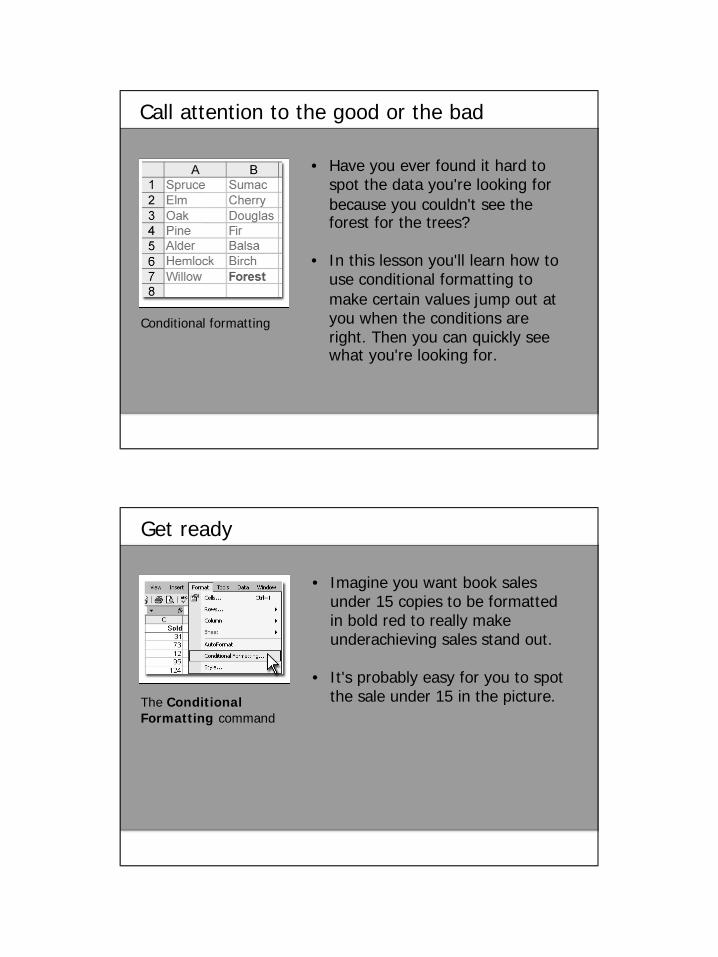
Call attention to the good or the bad
• Have you ever found it hard to spot the data you're looking for because you couldn't see the forest for the trees?
• In this lesson you'll learn how to use conditional formatting to make certain values jump out at you when the conditions are right. Then you can quickly see what you're looking for.
Conditional formatting
Get ready
• Imagine you want book sales under 15 copies to be formatted in bold red to really make underachieving sales stand out.
• It's probably easy for you to spot the sale under 15 in the picture. The Conditional
Formatting command

Get ready
1. Select column C (which contains the book sales numbers).
2. Click Conditional Formattingon the Format menu.
The Conditional Formatting command
But if this workbook had lots of other rows, the other under-15 entries could get lost in the rest of the data:
State your conditions
• The Conditional Formattingdialog box is big, with enough boxes and buttons to be intimidating, because it's built to take in a lot of possible conditions.
The Conditional Formatting dialog box.
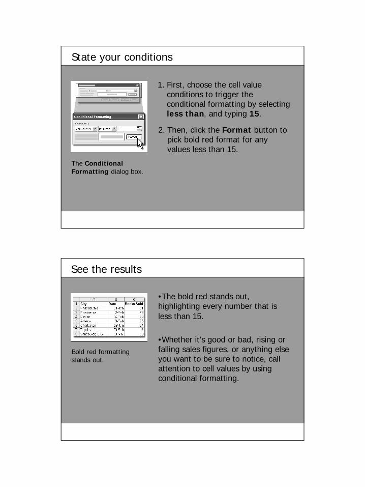
State your conditions
The Conditional Formatting dialog box.
1. First, choose the cell value conditions to trigger the conditional formatting by selecting less than, and typing 15.
2. Then, click the Format button to pick bold red format for any values less than 15.
See the results
•The bold red stands out, highlighting every number that is less than 15.
•Whether it's good or bad, rising or falling sales figures, or anything else you want to be sure to notice, call attention to cell values by using conditional formatting.
Bold red formatting stands out.

Suggestions for practice
1. Make text turn red under the right condition.
2. Add another condition.
3. Get rid of conditional formatting.
•Online practice (requires Excel 2003)
Test 5, question 1
• The first conditional formatting step is to select data before setting up your conditions. (Pick one answer.)
1. True.
2. False.
Test 5, question 1: Answer
• True.
• This is an important step that's easy to forget. For example, if the data that you want to apply conditional formatting to is in column C, select the cells in column C before you start.
Test 5, question 2
• Where is the Conditional Formatting command located? (Pick one answer.)
1. On the Format menu.
2. On the View menu.
3. On the Tools menu.

Test 5, question 2: Answer
• On the Format menu.
Test 5, question 3
• You can use up to two conditions in a cell or a given range of cells. (Pick one answer.)
1. True.
2. False.

Test 5, question 3: Answer
• False.
• Click the Add button in the Conditional Formattingdialog box to add up to two additional conditions to the original conditional formatting.
Test 3, question 4
• To get rid of conditional formatting, select the column it is in, and then: (Pick one answer.)
1. On the Format menu, click Conditional Formatting.
2. Right-click, and then select Conditional Formatting.
3. Right-click, and then select Delete Conditional Formatting.

Test 3, question 4: Answer
• On the Format menu, click Conditional Formatting.
• Then click Delete, and select the check boxes for the conditions you want to delete.
Microsoft® Office Excel® for the Public Works Professional
More Resources
For more details of the tasks covered in this course, visit http://office.microsoft.com. There, you will find help on all versions of Excel, including Excel 2003 and 2007.
Another great resource is http://exceluser.com, which has many additional business functions for Excel.