Microalgae culture to treat piggery

anaerobic digestion effluent

A thesis submitted in partial fulfilment for the award of the degree of

Honoursin Biotechnology

Jeremy AyreBBiotech

2013

I declare that this thesis is my own account of my research and contains workwhich has not been previously submitted for a degree at any tertiary institution.

Jeremy M Ayre

i

“You are capable of more than you know. Choose a goal that seems right for you

and strive to be the best, however hard the path. Aim high. Behave honourably.

Prepare to be alone at times, and to endure failure. Persist! The world needs all

you can give.”

Edward O. Wilson

This work is dedicated to my mother who has always supported me,

my father who has inspired my curiosity for science and my beautiful

wife Cheryl who has encouraged me to follow my dreams.

Jeremy 2013

ii

Abstract

The use of microalgae technology for the treatment of piggery anaerobic digestioneffluent offers attractive advantages over current wastewater treatment systemsused by Australian piggeries. These include recovery of nutrients in the form ofbiomass that might be used as pig feed or to enable the production of biofuel,better recycling of water, improved economic returns and better environmentaloutcomes.

This study utilised bioprospecting strategies which incorporated the selection andculture of algae species which were capable of growing on undiluted, untreatedpiggery anaerobic digestion effluent for this purpose. The successful isolation ofa Chlorella species using a synthetic medium containing 500 mg NH3-N.L�1 andthe operation of several raceway ponds over a course of 20 weeks with ammoniaconcentrations of up to 1,600 mg NH3-N.L�1 with a mixed algae culture provideddata to support the hypothesis that algae culture is not out of reach for thisapplication.

The data showed that high pH levels, temperature extremes and variable nutri-ent composition could be accommodated through the careful management of anoutdoor pond system. It was also found that some aspects of the algae growthperformance such as chlorophyll content can be improved by the addition of CO2

to the culture medium.

iii

Contents

Abstract iii

Acknowledgements vi

1 Introduction 1

1.1 Piggery wastewater treatment . . . . . . . . . . . . . . . . . . . . . 11.2 Characteristics of piggery anaerobic digestion effluent . . . . . . . . . 5

1.2.1 Ammonia . . . . . . . . . . . . . . . . . . . . . . . . . . . . 61.2.2 Turbidity and Phosphorous . . . . . . . . . . . . . . . . . . 71.2.3 Biochemical Oxygen Demand . . . . . . . . . . . . . . . . . 71.2.4 Chemical Oxygen Demand . . . . . . . . . . . . . . . . . . . 8

1.3 The potential of microalgae wastewater treatment . . . . . . . . . . . 81.3.1 Ammonia reactions and pH dynamics in algae culture . . . . . 101.3.2 Turbidity and Phosphorous . . . . . . . . . . . . . . . . . . 131.3.3 Pathogens . . . . . . . . . . . . . . . . . . . . . . . . . . . 13

1.4 Bioprospecting Strategies . . . . . . . . . . . . . . . . . . . . . . . . 141.4.1 Adaptation and Mutation . . . . . . . . . . . . . . . . . . . 15

1.5 Turbidity and Pond Design . . . . . . . . . . . . . . . . . . . . . . . 151.6 Summary and Aims of The Experiments . . . . . . . . . . . . . . . . 18

2 Materials and Methods 20

2.1 Chemicals and Solvents . . . . . . . . . . . . . . . . . . . . . . . . . 202.2 Algal Culturing . . . . . . . . . . . . . . . . . . . . . . . . . . . . . 20

2.2.1 Synthetic Media . . . . . . . . . . . . . . . . . . . . . . . . 202.2.2 Sterile Techniques . . . . . . . . . . . . . . . . . . . . . . . 232.2.3 Piggery anaerobic digestate based media . . . . . . . . . . . . 242.2.4 Setup of Sand Filter . . . . . . . . . . . . . . . . . . . . . . 25

2.3 Analytical Methods . . . . . . . . . . . . . . . . . . . . . . . . . . 282.3.1 Nutrient Characterisation . . . . . . . . . . . . . . . . . . . 282.3.2 Biomass . . . . . . . . . . . . . . . . . . . . . . . . . . . . 282.3.3 Chlorophyll determination . . . . . . . . . . . . . . . . . . . 292.3.4 Cell Count . . . . . . . . . . . . . . . . . . . . . . . . . . . 292.3.5 Ammonia determination . . . . . . . . . . . . . . . . . . . . 302.3.6 Temperature . . . . . . . . . . . . . . . . . . . . . . . . . . 302.3.7 pH . . . . . . . . . . . . . . . . . . . . . . . . . . . . . . . 30

2.4 Isolation of Algae Strains . . . . . . . . . . . . . . . . . . . . . . . . 302.4.1 Sources of Samples . . . . . . . . . . . . . . . . . . . . . . . 302.4.2 Bioprospecting Process . . . . . . . . . . . . . . . . . . . . . 332.4.3 Bioprospecting Culture Tanks . . . . . . . . . . . . . . . . . 34

2.5 Single species isolation on Agar plates . . . . . . . . . . . . . . . . . 382.6 Paddle wheel driven raceway ponds . . . . . . . . . . . . . . . . . . 38

2.6.1 Location and climate . . . . . . . . . . . . . . . . . . . . . . 382.6.2 Operating conditions . . . . . . . . . . . . . . . . . . . . . . 38

iv

2.6.3 Culture establishment phase . . . . . . . . . . . . . . . . . . 392.6.4 Batch and semicontinuous phase with high ammonia and CO2

addition . . . . . . . . . . . . . . . . . . . . . . . . . . . . 40

3 Microalgae bioprospecting 42

3.1 Introduction . . . . . . . . . . . . . . . . . . . . . . . . . . . . . . 423.2 Results . . . . . . . . . . . . . . . . . . . . . . . . . . . . . . . . . 433.3 Discussion . . . . . . . . . . . . . . . . . . . . . . . . . . . . . . . 53

4 Reliable long term outdoor cultivation 55

4.1 Introduction . . . . . . . . . . . . . . . . . . . . . . . . . . . . . . 554.2 Results . . . . . . . . . . . . . . . . . . . . . . . . . . . . . . . . . 56

4.2.1 Natural ammonia decrease in raceway ponds . . . . . . . . . . 584.2.2 Batch phase growth . . . . . . . . . . . . . . . . . . . . . . 594.2.3 Semicontinuous phase . . . . . . . . . . . . . . . . . . . . . 67

4.3 Discussion . . . . . . . . . . . . . . . . . . . . . . . . . . . . . . . 75

5 General conclusions 77

5.1 Future directions . . . . . . . . . . . . . . . . . . . . . . . . . . . . 78

Bibliography 81

v

Acknowledgements

Firstly I must thank my primary supervisor Dr Navid Moheimani for his un-wavering support and encouragement throughout this honours project and mysecondary supervisor Professor Michael Borowitzka. The advice and wisdomthey have both shared with me has been at times challenging and at other timesinspirational throughout 2013.

I also thank Josh Sweeny, Hugh Payne and the other staff who have been helpfuland accommodating on my visits to the Medina Research Station and the stu-dents at the Algae R & D Lab who have been welcoming assistants, tutors andconversationalists throughout the year.

My most humble thanks also to my wife Cheryl who has been an amazing sup-porter, advisor and always will be my best friend.

I owe a lot to all of you.

vi

Chapter 1

Introduction

1.1 Piggery wastewater treatment

The environmental impacts of intensive pig production can be significant. Apoorly managed piggery may risk wastewater pollution to local waterways, pro-duce offensive odour emissions and outlet greenhouse gases into the atmosphere(Maraseni and Maroulis, 2008). In contrast, a well managed piggery handles andreuses wastewater appropriately, maintains control of odour emissions and out-puts very little greenhouse gas (Maraseni and Maroulis, 2008; APL, 2011; O’Neilland Phillips, 1991; Vanotti et al., 2008). It has been claimed that productionof pig meat has the potential to be one of the most emission friendly sources ofanimal protein for the human diet (APL, 2010c).

Recent figures as of July 2009 indicate that 91% of pigs at Australian piggeries re-side on farms with large herds of more than 1000 animals (Pink, 2012). Wastew-ater generated through high intensity pig production is high in ammonia andphosphorous as well as has high chemical and biological oxygen demands (CODand BOD) (Olguin et al., 2003; Boursier et al., 2005; APL, 2011). High phos-phorous levels have been shown to correlate to high turbidity levels giving theeffluent a dark colour (Ong et al., 2006).

High COD and BOD presents a threat to water receiving outflows in terms of po-tential oxygen depletion (Fallowfield and Garrett, 1985). Such excessive levels ofpollutants can cause eutrophication in waterways, compromising a resource thatsupports wildlife and human populations (Carpenter et al., 1998; Woltemade,2000). In severe cases, blooms of cynobacteria as a result of high nutrient levelsin wastewater produce toxins that are lethal to livestock and humans (Ong et al.,

1

2006). Groundwater can also be at risk of contamination from misplaced piggeryeffluent (Svoboda, 1995; Krapac et al., 2002).

A wide variety of wastewater treatment methods are available that can be usedto reduce the available nutrient load in the effluent output from piggeries. Thesesystems may include a combination of aerobic treatment, anaerobic digestion,facultative ponds and evaporation ponds (Ahlberg and Boyko, 1972; Fenlon andMills, 1980; APL, 2010b; Buchanan et al., 2013).

Figure 1.1: A basic design of an aerobic treatment system. In this case anoxidation ditch system is integrated with extended treatment and disposal options(Ushikubo et al., 1991).

60 A. U S H I K U B O ET AL.

manure to the immediate area of its production (Young, 1980). On-site re- cycling alternatives include: animal bedding, animal rations, combustible fuel or biogas generation (Shaffer and van der Meulen, 1987; Japan Environmen- tal Agency, 1988).

OXIDATION DITCH TREATMENT SYSTEMS

The simplest oxidation ditch treatment systems are modifications of the activated sludge process. The most common of these is a single closed-loop channel, 1.2-1.5 m deep, ~ 3 m wide and 15 m long with one or more surface rotor type aerators (Barnes et al., 1983 ). The rotors serve two functions. They bring sufficient oxygen into the liquid to support the microbial population, and they mix and move the solids. A diagram of a simple oxidation channel system is presented in Fig. 1.

The original design of circular channel systems with surface aerators to aer- ate, mix and propel the treated wastewater was developed in the 1920s and 1930s. This method has undergone several modifications since the first fully operational oxidation ditches were introduced to treat municipal wastewater in The Netherlands in the late 1950s and the United Kingdom in 1963 (Fors- ter, 1983; Johnstone et al., 1983).

With the advent of new plastics during the late 1960s, rotating biological contactors (RBC) were developed that retain many advantages of the old rock trickling filters without some of their disadvantages. RBC systems were extensively employed in the mid and late 1970s. However, use of these sys- tems declined in the 1980s primarily because of structural problems related

\~ ~. receiving waters

oxidation pond or I// Final Disposal Options aerated lagoon ~ / ....

~ / .~- ~ / I / land application

I1'11 rotor ~ ~

return sludge excess sludge

Fig. 1. Oxidation ditch system integrated with extended treatment and disposal options.

One treatment system which is gaining acceptance in Australian piggeries isanaerobic digestion ponds. These systems typically consist of a covered pondcontaining wastewater which is biologically treated by heterotrophic microor-ganisms in the absence of oxygen (APL, 2010a). The covered digesters allow theproduction and capture of biogas including methane (CH4) and carbon dioxide(CO2) (Sowers, 2009; Buchanan et al., 2013). The benefits obtained in theseponds are, the removal of solids through settling, capture of biogas for use as abiofuel and the reduction of odour emissions (Leitão et al., 2006; APL, 2010b).

The utilisation of methane as a fuel source allows the ability to generate heatand other forms of energy for localised use (Lim and Headberry-Partners-P/L,2004; Dimpl, 2010). This can effectively reduce dependence on energy sourcesfrom outside the piggery such as the electric grid or fossil fuel. However, as CH4

2

is utilised, CO2, another green house gas (GHG) is produced. Ideally CO2 willbe captured and reused within the piggery, if a model incorporating CO2 uptakesuch as algae culture were to be adopted.

In recent decades awareness of the importance of piggery wastewater treatmentsystems has increased along with the use of anaerobic digestion ponds. Cur-rently around 83% of Australian piggeries use anaerobic digestion wastewatertreatment ponds as part of their wastewater treatment system (APL, 2010a)cited in (Buchanan et al., 2013).

Figure 1.2: Schematic of effluent management at Medina research station showingeffluent flow through covered anaerobic pond (CAP). (Image provided by HughPayne, WA Department of Agriculture and Food).

Schematic of effluent management at Medina RS showing effluent flow through covered anaerobic pond (CAP)

Pond 1(disused)

Pond 2

Pond 3 CAP

1. Holding Sump A 2. Run-down screen 3. Holding Sump B

3 1

2

Outlet from CAP through water level control sump to Pond 2

Gas pipeline to flare

Condensation trap and blower fan

Solar powered flare

CAP

Effluent Pathway a) Effluent drains from sheds into Tank 1 b) Pumped from Tank 1 over rundown screen and

drained into Tank 3 c) Pumped from Tank 3 into CAP as necessary d) Treated effluent displaced from CAP as effluent

enters e) Effluent drains from CAP into sump which

controls water level in CAP f) Drains from Sump into Pond 2

Gas Pathway i) Gas passes through collection ring ii) Gas drawn along pipeline to condensation trap iii) Blown through flare by 24volt fan iv) Biogas ignited at top of flare.

3

Figure 1.3: Photograph of the covered anaerobic pond at Medina research station.Some rainwater is visible on the surface of the pond cover and a small amount ofbiogas is trapped under the cover.

A recent review of wastewater management in Australian piggeries recommendedthat along with anaerobic digestion, microalgae culture systems should be inves-tigated further as a potential component of the Australian piggery wastewatermanagement strategy (Buchanan et al., 2013). Studies in the use of microalgaeculture as a wastewater treatment have been ongoing since the 1950’s (Oswaldand Gotaas, 1955; McGriff Jr and McKinney, 1972; Dor, 1975; Hashimoto andFurukawa, 1989) however these have failed to result in widespread applicationsfor the industry.

In the context of an Australian piggery system, anaerobic digestion is fast be-coming a more commonly recommended treatment in wastewater managementsystems (APL, 2010b). In order to integrate microalgae cultures into current pig-gery practices, the use of anaerobic digestion effluent as an algae growth mediawould be a sensible approach.

4

1.2 Characteristics of piggery anaerobic digestion ef-

fluent

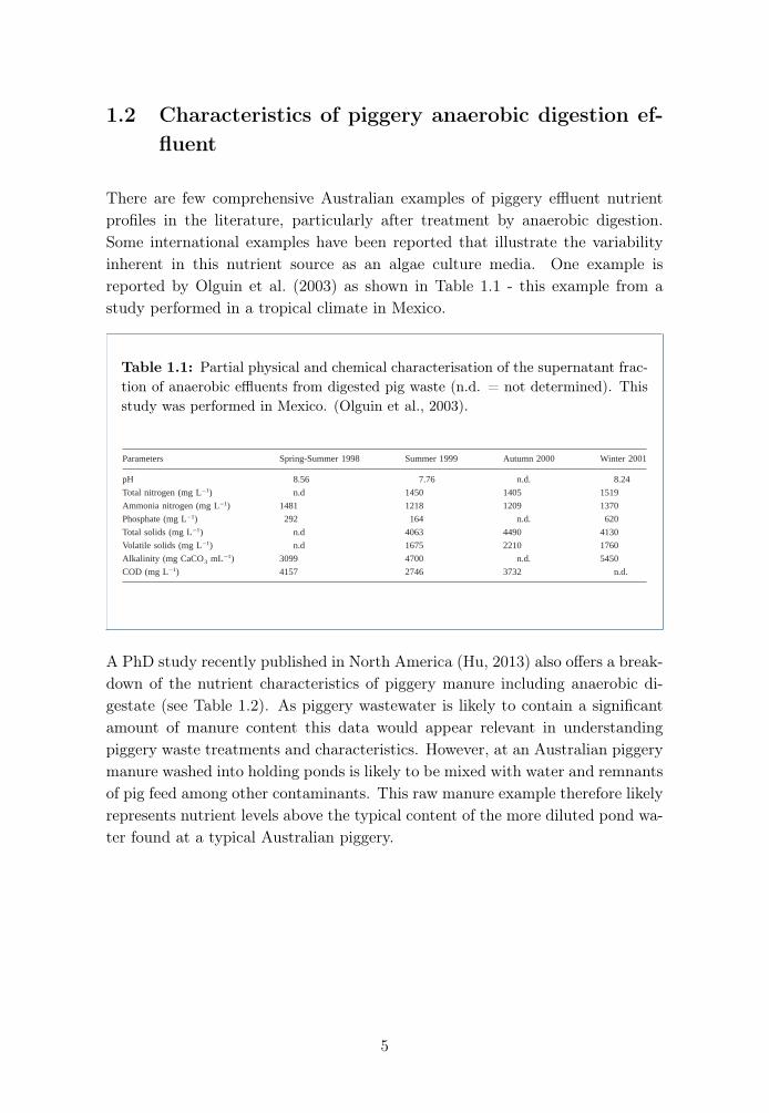
There are few comprehensive Australian examples of piggery effluent nutrientprofiles in the literature, particularly after treatment by anaerobic digestion.Some international examples have been reported that illustrate the variabilityinherent in this nutrient source as an algae culture media. One example isreported by Olguin et al. (2003) as shown in Table 1.1 - this example from astudy performed in a tropical climate in Mexico.

Table 1.1: Partial physical and chemical characterisation of the supernatant frac-tion of anaerobic effluents from digested pig waste (n.d. = not determined). Thisstudy was performed in Mexico. (Olguin et al., 2003).

raceways (23.6 m2 or 6.03 m2) which were agitatedby a paddle wheel. The length width ratio was 1:10for both sizes of raceway. Two of the larger pondswere utilised during 1998 and 1999, two of thesmaller ponds were utilised during 2000 and 2001.Eight different Spirulina batch cultures were estab-lished during spring and summer 1998. Three differ-ent groups of outdoor semi-continuous cultures werecarried out. Group 1 was operated from May to June1999 (summer). Group 2 was operated from Septem-ber to October 2000 (autumn), and Group 3 fromFebruary to March 2001 (winter).

Three weeks before the first experimental cycle, aninoculum of the mixed Spirulina culture grown insynthetic medium was added to the pond to provide25% of the total volume. Subsequently, 75% of thepond’s volume was processed every 6–7 days and thesame volume of freshly prepared culture medium wasadded, establishing a semi-continuous culture. Agita-tion was provided from 0600 to 1800 h and pondswere covered with a polyethylene sheet from 1800 to0800 h. Evaporation was counteracted by adding ev-ery morning,the same volume of fresh water. Shadeswere located over ponds from 1200 to 1700 h to avoidexcess of solar radiation.

Climatic conditions

Light intensity and temperature were recorded dailyat: 1000, 1300 and 1700 for 1999. 1000, 1200, 1400and 1600 h for 2000 and 2001. The light intensity wasmeasured by a digital light meter (Luxtron LX-101).

Analytical methods

Total solids, volatile solids, moisture, alkalinity, totalN and NH4-N were determined according to the

APHA (1998). Under the technic conditions (pH 7.0and 20 °C), NH4-N is by far, the dominant form ofammonia nitrogen (NH3 is in a concentration below0.074 mg/L). Dry weight and protein were deter-mined according to Olguín et al. (1997). Phosphatewas determined according to Hach Company (1995).Pond water samples for determination of NH4-N andPO4-P were obtained by filtration with Whatman No.4 paper.

Statistical analysis

The effects of pond depth on productivity, proteincontent and nutrient removal were analysed usingANOVA parametric test. The analysis was performedusing STATISTICA Program (version 5.5, 1996) atthe P = 0.05 level.

Results

Quality of anaerobic effluents from digested pigwaste

A partial physical and chemical characterisation of allsamples of the supernatant of the anaerobic effluentsfrom digested pig waste showed no major differencesbetween years (Table 1). The pH was always alkaline(around 8.3) and the alkalinity was above 3000 mgCa CO3 mL−1 (ensuring a supply of bicarbonate ionsto medium at pH 9.5). NH4-N accounted > 90% totalN.

Table 1. Partial physical and chemical characterisation of the supernatant fraction of anaerobic effluents from digested pig waste (n.d. = notdetermined; COD = chemical oxygen demand).

Parameters Spring-Summer 1998 Summer 1999 Autumn 2000 Winter 2001

pH 8.56 7.76 n.d. 8.24Total nitrogen (mg L−1) n.d 1450 1405 1519Ammonia nitrogen (mg L−1) 1481 1218 1209 1370Phosphate (mg L−1) 292 164 n.d. 620Total solids (mg L−1) n.d 4063 4490 4130Volatile solids (mg L−1) n.d 1675 2210 1760Alkalinity (mg CaCO3 mL−1) 3099 4700 n.d. 5450COD (mg L−1) 4157 2746 3732 n.d.

251

A PhD study recently published in North America (Hu, 2013) also offers a break-down of the nutrient characteristics of piggery manure including anaerobic di-gestate (see Table 1.2). As piggery wastewater is likely to contain a significantamount of manure content this data would appear relevant in understandingpiggery waste treatments and characteristics. However, at an Australian piggerymanure washed into holding ponds is likely to be mixed with water and remnantsof pig feed among other contaminants. This raw manure example therefore likelyrepresents nutrient levels above the typical content of the more diluted pond wa-ter found at a typical Australian piggery.

5

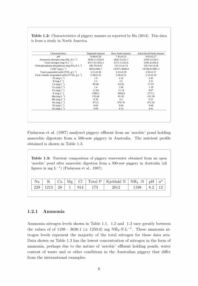
Table 1.2: Characteristics of piggery manure as reported by Hu (2013). This datais from a study in North America.

26##

UMN245 Jun, 2006 Lake Ripley picnic area, Lithfield UMN275 Jul, 2006 Amelia Lake

UMN246 Jun, 2006 Pond between County Rd 1 and County Rd 23,

Litchfield UMN276 Jul, 2006 Coon Rapids Dam #1 UMN247 Jun, 2006 Lake Hope, Litchfield UMN277 Jul, 2007 Pond at Marine City

UMN250 Jun, 2006 Theodore Wirth Parkway, Pond #3 on the right

coming from 394 UMN278 Jul, 2007 Pond at Marine City

UMN251 Jun, 2006 Theodore Wirth Parkway, left, right Pond #2b

around the bridge UMN279 Jul, 2007 Spring brook 1, Fridley UMN252 Jun, 2006 Theodore Wirth Lake 1, farther than the beach UMN281 May, 2006 Itasca main lake

Table 5 Characteristics of swine manure

Characteristics Digested manure Raw fresh manure Autoclaved fresh manure pH 8.48±0.29 7.45±0.31 9.63±0.27

Ammonia-nitrogen (mg NH3-N L-1) 3630.1±1250.0 2820.3±225.7 2594.3±534.3 Total nitrogen (mg N L-1 ) 4317.0±1263.2 3272.1±323.6 3196.4±456.4

Orthophosphate-phosphorus (mg PO4-P L-1) 100.70±9.91 131.51±6.74 150.74±14.26 CODa (mg L-1) 8933±666.7 14707±3668.9 14748.9±3891.1

Total suspended solid (TSS, g L-1) 3.21±0.36 3.23±0.29 2.92±0.17 Total volatile suspended solid (TVSS, g L-1) 2.38±0.25 2.50±0.31 2.15±0.18

Al (mg L-1) 1.9 2.32 2.45 B (mg L-1) 2.5 2.5 3.21 Ca (mg L-1) 99.46 64.02 57.67 Cu (mg L-1) 1.4 1.06 1.18 Fe (mg L-1) 11.66 11.14 8.67 K (mg L-1) 3389.2 3494.8 3772.1

Mg (mg L-1) 133.66 81.92 101.38 Mn (mg L-1) 0.38 0.2 0.31 Na (mg L-1) 973.5 970.76 972.43 Ni (mg L-1) 0.64 0.64 0.68 Zn (mg L-1) 4.94 4.14 4.41

CODa is short for Chemical Oxygen Demand.

Finlayson et al. (1987) analysed piggery effluent from an ‘aerobic’ pond holdinganaerobic digestate from a 500-sow piggery in Australia. The nutrient profileobtained is shown in Table 1.3.

Table 1.3: Nutrient composition of piggery wastewater obtained from an open‘aerobic’ pond after anaerobic digestion from a 500-sow piggery in Australia (allfigures in mg L�1) (Finlayson et al., 1987):

Na K Ca Mg Cl Total P Kjeldahl N NH4 -N pH na

229 1213 28 1 914 173 2012 1198 8.2 12

1.2.1 Ammonia

Ammonia nitrogen levels shown in Table 1.1, 1.2 and 1.3 vary greatly betweenthe values of of 1198 - 3630.1 (± 1250.0) mg NH3-N.L�1. These ammonia ni-trogen levels represent the majority of the total nitrogen for these data sets.Data shown on Table 1.3 has the lowest concentration of nitrogen in the form ofammonia, perhaps due to the nature of ‘aerobic’ effluent holding ponds, watercontent of waste and or other conditions in the Australian piggery that differfrom the international examples.

6

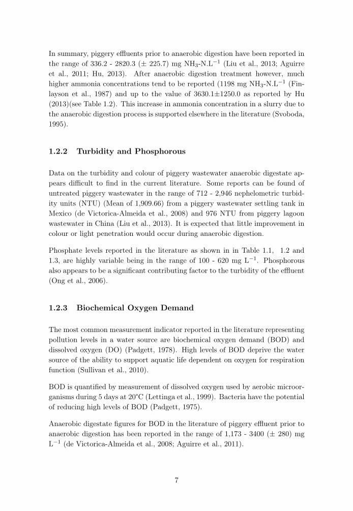
In summary, piggery effluents prior to anaerobic digestion have been reported inthe range of 336.2 - 2820.3 (± 225.7) mg NH3-N.L�1 (Liu et al., 2013; Aguirreet al., 2011; Hu, 2013). After anaerobic digestion treatment however, muchhigher ammonia concentrations tend to be reported (1198 mg NH3-N.L�1 (Fin-layson et al., 1987) and up to the value of 3630.1±1250.0 as reported by Hu(2013)(see Table 1.2). This increase in ammonia concentration in a slurry due tothe anaerobic digestion process is supported elsewhere in the literature (Svoboda,1995).

1.2.2 Turbidity and Phosphorous

Data on the turbidity and colour of piggery wastewater anaerobic digestate ap-pears difficult to find in the current literature. Some reports can be found ofuntreated piggery wastewater in the range of 712 - 2,946 nephelometric turbid-ity units (NTU) (Mean of 1,909.66) from a piggery wastewater settling tank inMexico (de Victorica-Almeida et al., 2008) and 976 NTU from piggery lagoonwastewater in China (Liu et al., 2013). It is expected that little improvement incolour or light penetration would occur during anaerobic digestion.

Phosphate levels reported in the literature as shown in in Table 1.1, 1.2 and1.3, are highly variable being in the range of 100 - 620 mg L�1. Phosphorousalso appears to be a significant contributing factor to the turbidity of the effluent(Ong et al., 2006).

1.2.3 Biochemical Oxygen Demand

The most common measurement indicator reported in the literature representingpollution levels in a water source are biochemical oxygen demand (BOD) anddissolved oxygen (DO) (Padgett, 1978). High levels of BOD deprive the watersource of the ability to support aquatic life dependent on oxygen for respirationfunction (Sullivan et al., 2010).

BOD is quantified by measurement of dissolved oxygen used by aerobic microor-ganisms during 5 days at 20°C (Lettinga et al., 1999). Bacteria have the potentialof reducing high levels of BOD (Padgett, 1975).

Anaerobic digestate figures for BOD in the literature of piggery effluent prior toanaerobic digestion has been reported in the range of 1,173 - 3400 (± 280) mgL�1 (de Victorica-Almeida et al., 2008; Aguirre et al., 2011).

7

1.2.4 Chemical Oxygen Demand

Similar to BOD, the Chemical Oxygen Demand (COD) parameter is a measure-ment of pollution in terms of the total concentration of substances that can bechemically oxidised in the water. This value is expressed in mg O2 per litre(Pisarevsky et al., 2005).

The COD figures reported in the data cited in in Table 1.1 and 1.2 piggeryanaerobic digestate, ranges from 2746 - 8933 (± 666.7) (Olguin et al., 2003; Hu,2013).

1.3 The potential of microalgae wastewater treatment

The utilisation of piggery wastewater as an algae culture media has been investi-gated over several decades with some success reported under various laboratoryand field conditions. Factors that currently limit the adoption of algae culture inthis context include the turbidity and colour of piggery wastewater (Buchananet al., 2013; Barlow et al., 1975), high ammonia levels (Finlayson et al., 1987)and high pH (Azov and Goldman, 1982). The combination of high ammonia andpH levels shifts the chemical equilibrium of the nutrient mix from NH+

4 towardNH3 which has a generally toxic effect on most algae species (as per Figure 1.6)and also limits the availability of CO2 to the algae culture (Azov and Goldman,1982; Källqvist and Svenson, 2003).

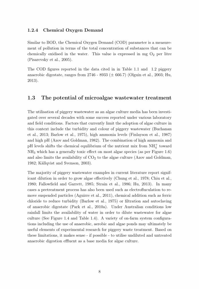
The majority of piggery wastewater examples in current literature report signif-icant dilution in order to grow algae effectively (Chung et al., 1978; Chiu et al.,1980; Fallowfield and Garrett, 1985; Strain et al., 1986; Hu, 2013). In manycases a pretreatment process has also been used such as electrofluculation to re-move suspended particles (Aguirre et al., 2011), chemical addition such as ferricchloride to reduce turbidity (Barlow et al., 1975) or filtration and autoclavingof anaerobic digestate (Park et al., 2010a). Under Australian conditions lowrainfall limits the availability of water in order to dilute wastewater for algaeculture (See Figure 1.4 and Table 1.4). A variety of on-farm system configura-tions including the use of anaerobic, aerobic and algae ponds may ultimately beuseful elements of experimental research for piggery waste treatment. Based onthese limitations, it makes sense - if possible - to utilise undiluted and untreatedanaerobic digestion effluent as a base media for algae culture.

8

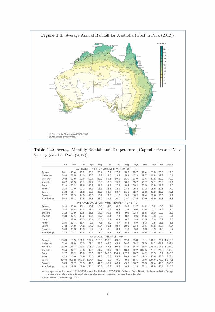
Figure 1.4: Average Annual Rainfall for Australia (cited in Pink (2012))

80 Year Book Australia 2012

an average of 2,942 mm over 66 years; short-term records suggest that other parts of the region have an average near 3,500 mm.

The Snowy Mountains area in New South Wales also has a particularly high rainfall. While there are no official rain gauges in the wettest areas on the western slopes above 1,800 metres elevation, runoff data suggest that the average annual rainfall in parts of this region exceeds 3,000 mm. Small pockets with averages exceeding 2,500 mm also occur in the north-east Victorian highlands and some parts of the east coastal slopes.

SeasonalAustralia’s rainfall pattern is strongly seasonal in character, with a winter rainfall regime in parts of the south, a summer regime in the north and generally more uniform or erratic throughout the year elsewhere. Major rainfall zones include:

� The marked wet summer and dry winter of northern and north-western Australia. In this

region, winters are normally almost completely dry (e.g. Darwin in table 1.5), except near exposed eastern coastlines.

� The wet summer and relatively (but not completely) dry winter of south-eastern Queensland and north-eastern New South Wales (e.g. Brisbane in table 1.5).

� Fairly uniform rainfall in south-eastern Australia, including most of New South Wales, parts of Victoria and eastern Tasmania (e.g. Sydney, Melbourne, Canberra and Hobart in table 1.5). The exact seasonal distribution can be influenced by local topography, for example, winter is the wettest season at Albury on the windward side of the Snowy Mountains, but the driest season at Cooma on the leeward side.

� A marked wet winter and dry summer (sometimes called a ‘Mediterranean’ climate). This climate is most prominent in south-western Western Australia and southern South

1.4 AVERAGE ANNUAL RAINFALL FOR AUSTRALIA(a)

(a) Based on the 30 year period 1961–1990. Source: Bureau of Meteorology

Table 1.4: Average Monthly Rainfall and Temperatures, Capital cities and AliceSprings (cited in Pink (2012))

Chapter 1 — Geography and climate 81

Australia (e.g. Adelaide, Perth in table 1.5), but there is also a winter rainfall maximum in some other parts of the south-east, particularly those areas exposed to westerly or south-westerly winds, such as western Tasmania and south-western Victoria.

� Low and erratic rainfall through much of the western and central inland. Rainfall events are irregular and can occur in most seasons, but are most common in summer (e.g. Alice Springs in table 1.5).

Rain days and extreme rainfallsThe frequency of rain days (defined as days when 0.2 mm or more of rainfall is recorded in a 24-hour period) is greatest near the southern Australian coast, exceeding 150 rain days per year

in much of Tasmania, southern Victoria and the far south-west of Western Australia, peaking at over 250 per year in western Tasmania. Values exceeding 150 per year also occur along parts of the north Queensland coast. At the other extreme, a large part of inland western and central Australia has fewer than 25 rain days per year, and most of the continent away from the coasts has fewer than 50 per year. In the high rainfall areas of northern Australia away from the east coast, the number of rain days is typically about 80 to 120 per year, but rainfall events are likely to be heavier in this region than in southern Australia.

The highest daily rainfalls have occurred in the northern half of Australia and along the east coast, most of them arising from tropical cyclones, or further south-east coast lows, near

1.5 AVERAGE MONTHLY RAINFALL AND TEMPERATURES(a), Capital cities and Alice SpringsJan Feb Mar Apr May Jun Jul Aug Sep Oct Nov Dec Annual

AVERAGE DAILY MAXIMUM TEMPERATURE (°C) Sydney 26.1 26.4 25.2 23.1 20.4 17.7 17.2 18.5 20.7 22.4 23.6 25.6 22.3Melbourne 25.8 26.5 24.0 20.5 17.3 14.4 13.9 15.3 17.3 19.7 21.8 24.2 20.1Brisbane 29.2 28.8 28.0 26.1 23.5 21.1 20.6 21.6 23.9 25.5 27.1 28.6 25.3Adelaide 28.7 29.3 26.1 22.2 18.8 16.0 15.2 16.5 18.7 21.7 24.7 26.8 22.1Perth 31.9 32.2 29.8 25.9 21.8 18.9 17.9 18.4 20.2 22.5 25.8 29.2 24.5Hobart 21.8 22.0 20.2 17.9 15.1 12.3 12.2 13.4 15.3 17.2 18.6 20.3 17.2Darwin 31.8 31.4 31.8 32.8 32.2 30.7 30.7 31.5 32.7 33.3 33.3 32.6 32.1Canberra 27.7 27.3 24.5 20.0 15.9 12.3 11.5 13.2 16.2 19.4 22.6 26.3 19.7Alice Springs 36.4 35.1 32.8 27.8 23.2 19.7 20.0 23.0 27.5 30.9 33.9 35.8 28.8

AVERAGE DAILY MINIMUM TEMPERATURE (°C)Sydney 19.4 19.6 18.1 15.2 12.5 9.6 8.6 9.5 11.7 14.2 16.0 18.3 14.4Melbourne 15.4 15.8 14.3 11.7 9.8 7.6 6.8 7.6 9.0 10.5 12.2 13.9 11.2Brisbane 21.2 20.9 19.5 16.8 14.2 10.8 9.5 9.9 12.4 15.5 18.0 19.9 15.7Adelaide 16.8 17.1 15.2 12.1 10.2 8.1 7.4 8.2 9.6 11.5 13.8 15.5 12.1Perth 17.2 17.8 16.3 13.4 10.8 9.1 8.4 8.5 9.3 10.5 13.0 15.2 12.5Hobart 12.5 12.7 11.4 9.6 7.6 5.2 4.7 5.5 6.9 8.3 9.8 11.3 8.8Darwin 24.8 24.9 24.6 24.2 22.4 20.1 19.4 20.9 23.4 25.1 25.6 25.5 23.4Canberra 13.3 13.3 10.9 6.7 3.7 0.8 –0.1 1.0 3.6 6.3 8.9 11.6 6.7Alice Springs 21.3 20.7 17.4 12.3 8.2 4.8 3.8 6.2 10.4 14.6 17.9 20.2 13.2

AVERAGE RAINFALL (mm)Sydney 136.3 130.9 151.2 127.7 110.0 126.8 69.6 92.0 68.8 88.1 101.7 73.4 1 276.5Melbourne 52.4 49.0 40.0 52.1 58.8 48.6 45.1 54.6 59.2 69.5 64.2 61.1 654.4Brisbane 158.6 174.3 125.3 108.7 115.7 53.1 60.1 37.2 34.8 96.8 106.0 119.6 1 194.0Adelaide 19.4 12.7 26.6 42.0 61.2 79.7 79.9 68.0 62.2 347.5 29.7 27.8 563.0Perth 12.7 18.2 15.9 36.5 92.8 145.5 154.1 117.3 76.7 44.2 26.5 7.2 745.3Hobart 47.3 40.0 41.9 44.2 38.6 37.5 53.7 59.2 48.7 48.3 50.6 56.5 576.4Darwin 499.8 336.2 376.3 104.4 23.2 1.6 0.5 8.0 15.5 76.6 134.0 270.9 1 847.1Canberra 66.3 52.7 50.3 49.3 44.6 38.4 46.4 49.2 56.7 60.9 67.4 47.8 630.0Alice Springs 41.3 48.5 47.9 24.1 20.6 15.2 14.3 9.2 11.3 23.2 29.8 40.1 325.6

(a) Averages are for the period (1971–2000) except for Adelaide (1977–2000). Brisbane, Perth, Darwin, Canberra and Alice Springs averages are for observations taken at airports, others are at locations in or near the central city.

Source: Bureau of Meteorology 2003.

9

1.3.1 Ammonia reactions and pH dynamics in algae culture

Outdoor algae culture media are known to reach a pH level of up to 11 duringthe day under some conditions (Brewer and Goldman, 1976; Moheimani andBorowitzka, 2006). This appears to be due to a number of factors which canhave an impact on the pH of the algae growth medium including uptake of CO2

by algae during growth (Moheimani and Borowitzka, 2011) or other changes innutrient levels. For example Brewer and Goldman (1976) reports that nitrateassimilation leads to an output of OH� (raising pH) ions whereas ammoniaassimilation (via the ammonium ion) leads to an output of H+ ions (loweringthe pH). Bacterial denitrification and aerobic decomposition can also raise thepH (see Table 1.6). Rudd et al. (1988) found in one study that lake watermay be forced toward production of ammonium rather than nitrate under acidicconditions.

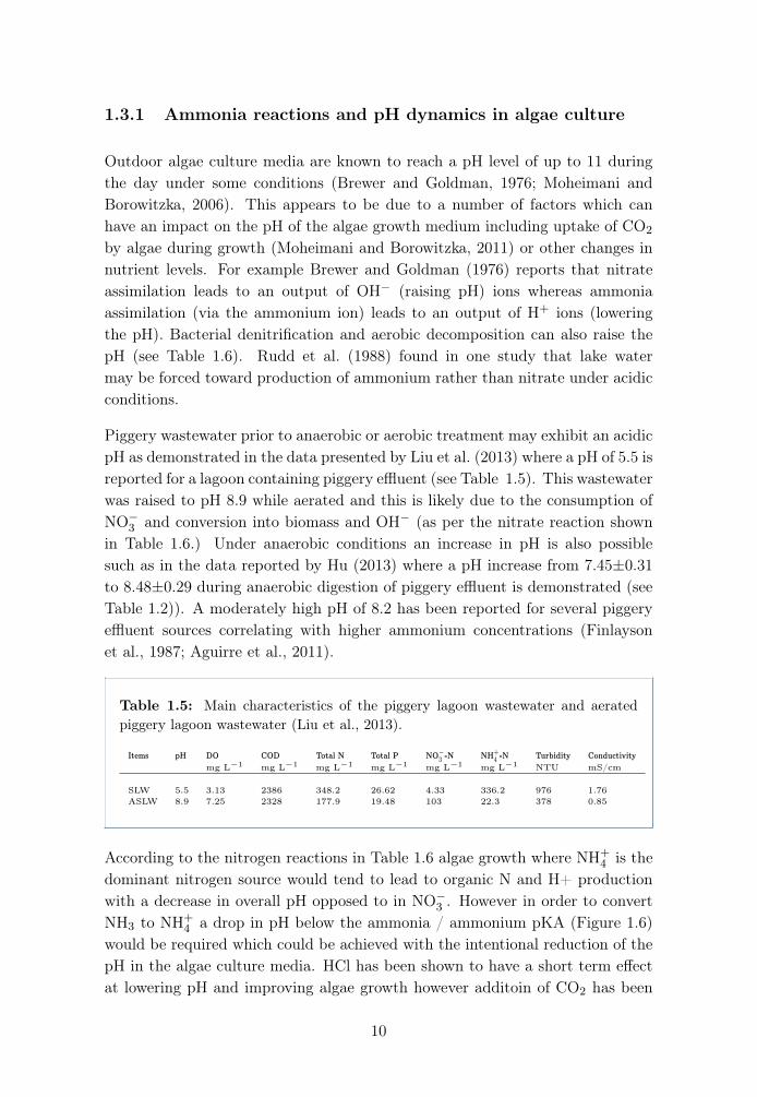
Piggery wastewater prior to anaerobic or aerobic treatment may exhibit an acidicpH as demonstrated in the data presented by Liu et al. (2013) where a pH of 5.5 isreported for a lagoon containing piggery effluent (see Table 1.5). This wastewaterwas raised to pH 8.9 while aerated and this is likely due to the consumption ofNO�

3 and conversion into biomass and OH� (as per the nitrate reaction shownin Table 1.6.) Under anaerobic conditions an increase in pH is also possiblesuch as in the data reported by Hu (2013) where a pH increase from 7.45±0.31to 8.48±0.29 during anaerobic digestion of piggery effluent is demonstrated (seeTable 1.2)). A moderately high pH of 8.2 has been reported for several piggeryeffluent sources correlating with higher ammonium concentrations (Finlaysonet al., 1987; Aguirre et al., 2011).

Table 1.5: Main characteristics of the piggery lagoon wastewater and aeratedpiggery lagoon wastewater (Liu et al., 2013).

Items pH DO COD Total N Total P NO�3 -N NH+

4 -N Turbidity Conductivitymg L�1 mg L�1 mg L�1 mg L�1 mg L�1 mg L�1 NTU mS/cm

SLW 5.5 3.13 2386 348.2 26.62 4.33 336.2 976 1.76ASLW 8.9 7.25 2328 177.9 19.48 103 22.3 378 0.85

According to the nitrogen reactions in Table 1.6 algae growth where NH+4 is the

dominant nitrogen source would tend to lead to organic N and H+ productionwith a decrease in overall pH opposed to in NO�

3 . However in order to convertNH3 to NH+

4 a drop in pH below the ammonia / ammonium pKA (Figure 1.6)would be required which could be achieved with the intentional reduction of thepH in the algae culture media. HCl has been shown to have a short term effectat lowering pH and improving algae growth however additoin of CO2 has been

10

shown to be much more effective for longer term results (Moheimani, 2012). Dueto the likely availability of end products from a biogas combustion localised at apiggery undergoing anaerobic digestion and biogas capture for heating or flaring,the CO2 content of biogas might serve as a useful pH lowering agent. Studieshave shown no inhibition of algae growth due to the use of flue gas (Hamasakiet al., 1994; Yun et al., 1997; Douskova et al., 2009; Moheimani, 2012).

Table 1.6: Schematic reactions for nitrogen up-take and the effects on pH andalkalinity (Brewer and Goldman, 1976).

Simplified Biological Effect on pH andReaction Alkalinity

Nitrogen assimilation (all microbes)

NitrateNO�

3 ! Org N + OH� increase(biomass)

AmmoniaNH+

4 ! Org N + H+ decrease(biomass)

Dissolved organic nitrogen (DON)DON ! Org N none

(biomass)

Aerobic decompositionOrg N ! NH+

4 + OH� increase(biomass)

Bacterial nitrification

NH+4 ! NO�

3 + 2H+ decrease

Bacterial denitrification

NO�3 ! N2 + OH� increase

Nitrogen fixationN2 ! Org N none

(biomass)

11

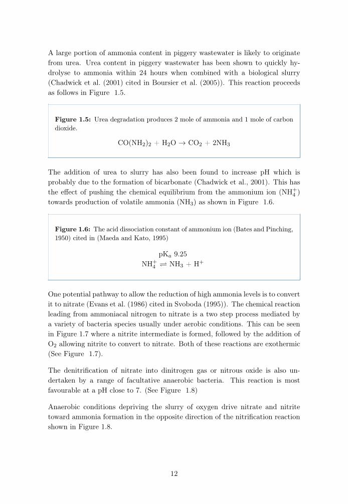
A large portion of ammonia content in piggery wastewater is likely to originatefrom urea. Urea content in piggery wastewater has been shown to quickly hy-drolyse to ammonia within 24 hours when combined with a biological slurry(Chadwick et al. (2001) cited in Boursier et al. (2005)). This reaction proceedsas follows in Figure 1.5.

Figure 1.5: Urea degradation produces 2 mole of ammonia and 1 mole of carbondioxide.

CO(NH2)2 + H2O ! CO2 + 2NH3

The addition of urea to slurry has also been found to increase pH which isprobably due to the formation of bicarbonate (Chadwick et al., 2001). This hasthe effect of pushing the chemical equilibrium from the ammonium ion (NH+

4 )towards production of volatile ammonia (NH3) as shown in Figure 1.6.

Figure 1.6: The acid dissociation constant of ammonium ion (Bates and Pinching,1950) cited in (Maeda and Kato, 1995)

pKa 9.25NH+

4 ⌦ NH3 + H+

One potential pathway to allow the reduction of high ammonia levels is to convertit to nitrate (Evans et al. (1986) cited in Svoboda (1995)). The chemical reactionleading from ammoniacal nitrogen to nitrate is a two step process mediated bya variety of bacteria species usually under aerobic conditions. This can be seenin Figure 1.7 where a nitrite intermediate is formed, followed by the addition ofO2 allowing nitrite to convert to nitrate. Both of these reactions are exothermic(See Figure 1.7).

The denitrification of nitrate into dinitrogen gas or nitrous oxide is also un-dertaken by a range of facultative anaerobic bacteria. This reaction is mostfavourable at a pH close to 7. (See Figure 1.8)

Anaerobic conditions depriving the slurry of oxygen drive nitrate and nitritetoward ammonia formation in the opposite direction of the nitrification reactionshown in Figure 1.8.

12

Figure 1.7: Nitrification of ammonia to nitrogen in a two step reaction (performedoptimally at pH 7.2 - 8.2) (Sharma and Ahlert, 1977) cited in (Svoboda, 1995).

NH+4 + 1.5 O2 ! 2H+ + H2O + NO�

2 + 58 to 84kcal (1)NO�

2 + 0.5 O2 ! NO�3 + 15.4 to 20.9kcal (2)

Figure 1.8: The denitrification reaction (performed optimally at pH 6 - 9)(Svo-boda, 1995).

NO�3 < > NO�

2 > N2O > N2

1.3.2 Turbidity and Phosphorous

The precipitation of dissolved organic matter using ferric chloride or throughfiltration utilising activated carbon has shown improvement in colour and lightpenetration of piggery effluent. This, however has also correlated with a markeddecrease in phosphorous availability for algae growth (Barlow et al., 1975). Datareported by Hu (2013) also indicated that during anaerobic digestion of piggerymanure the availability of phosphorous decreases (Table 1.2).

1.3.3 Pathogens

If algae biomass is to be collected from piggery wastewater with the intention tobe used as pig feed or if wastewater is to be reclaimed and reused within the pig-gery, the risks associated with disease transmission should be carefully evaluated(Buchanan et al., 2013). Pathogens that could present a risk of circulation andreinfection through piggery wastewater include Porcine circovirus, Hepatitis E,porcine parvovirus, Enterotoxigenic Escherichia coli, Salmonella sp., Clostridiumperfringens (Buchanan et al., 2013; Ramírez et al., 2005; Cordero et al., 2010;Payne, 1984). Treatments that ensure the sterilisation or use of waste outsidethe piggery to break the infection cycle are likely to be necessary. The potentialpathways for pathogen transport are indicated in Figure 1.9. The tendency ofalgal culture to drift toward a high pH may reduce algal productivity but couldbe beneficial for pathogen removal (Buchanan et al., 2013).

13

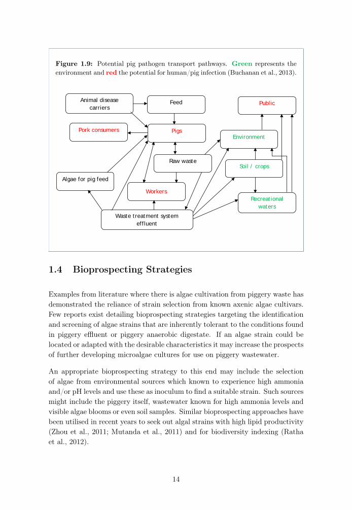
Figure 1.9: Potential pig pathogen transport pathways. Green represents theenvironment and red the potential for human/pig infection (Buchanan et al., 2013).

159

the microbiological quality of pig slurry and manure (Chinivasagam, Thomas et al. 2004).

In fact, little published information on pathogen numbers is pig slurry exists at all (Table

9.5).

Figure 9.1 Potential pig pathogen transport pathways. Green represents the environment and

red the potential for human/pig infection

Soil / crops

Pork consumers

Public Feed

Pigs

Recreational

waters

Raw waste

Workers

Environment

Waste treatment system

effluent

Animal disease

carriers

Algae for pig feed

1.4 Bioprospecting Strategies

Examples from literature where there is algae cultivation from piggery waste hasdemonstrated the reliance of strain selection from known axenic algae cultivars.Few reports exist detailing bioprospecting strategies targeting the identificationand screening of algae strains that are inherently tolerant to the conditions foundin piggery effluent or piggery anaerobic digestate. If an algae strain could belocated or adapted with the desirable characteristics it may increase the prospectsof further developing microalgae cultures for use on piggery wastewater.

An appropriate bioprospecting strategy to this end may include the selectionof algae from environmental sources which known to experience high ammoniaand/or pH levels and use these as inoculum to find a suitable strain. Such sourcesmight include the piggery itself, wastewater known for high ammonia levels andvisible algae blooms or even soil samples. Similar bioprospecting approaches havebeen utilised in recent years to seek out algal strains with high lipid productivity(Zhou et al., 2011; Mutanda et al., 2011) and for biodiversity indexing (Rathaet al., 2012).

14

1.4.1 Adaptation and Mutation

Through the use of mixed or axenic algae strains as starting cultures, it may bepossible to adapt towards an increased tolerance of high ammonia and high pHconditions. Ultimately the selection of the most productive strains and furtherrefinements to growth conditions may have the potential to develop a thrivingcultivation process with suitable biomass productivity.

Research on algal mutation and adaptation in an initially hostile environment hasshown that rare spontaneous mutations can arise giving favourable characteristicsthat improve survival (Lopez-Rodas et al., 2001; Costas et al., 2007; Sánchez-Fortún et al., 2009). Alternatively a culture of sexually reproductive algae strainsmight naturally tend to give rise to significant genetic diversity and encouragethe possibility of genetic recombination through naturally occurring haploid /diploid sexual life cycles which give rise to desirable characteristics that suitpiggery anaerobic digestion effluent (Hoshaw, 1961; Gupta and Agrawal, 2007).

A genetic engineering approach would also be worth consideration if ethicallyviable (Beer et al., 2009). Whatever the approach, through the optimisationof genetic diversity and successive re-inoculation of diverse algae strains underthe desired growth conditions the strong selection pressure should encouragethe survival of algae varieties which are capable of surviving under the desiredconditions.

1.5 Turbidity and Pond Design

A variety of algal pond designs and reactor chambers have been reported in theliterature including common configurations such as those listed below (Borow-itzka, 1999):

• Shallow open-air ponds with no artificial mixing,

• Outdoor ponds mixed by paddle-wheel,

• Circular outdoor ponds mixed by rotating arm,

• Indoor transparent carboys of approximately 20-40L volume, and

• Outdoor photobioreactors.

One of the most common designs, the outdoor pond mixed by paddle-wheel isoften known as a raceway pond. These can reach sizes up to 1ha per single pond

15

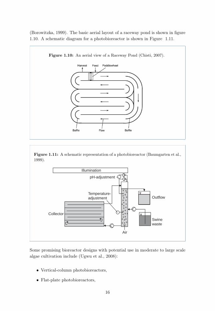
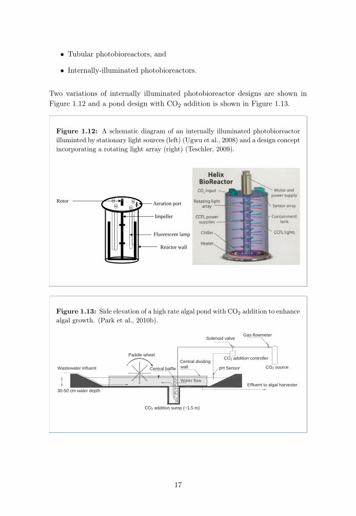
(Borowitzka, 1999). The basic aerial layout of a raceway pond is shown in figure1.10. A schematic diagram for a photobioreactor is shown in Figure 1.11.

Figure 1.10: An aerial view of a Raceway Pond (Chisti, 2007).

Production of algal oils requires an ability toinexpensively produce large quantities of oil-richmicroalgal biomass.

3. Microalgal biomass production

Producing microalgal biomass is generally moreexpensive than growing crops. Photosynthetic growthrequires light, carbon dioxide, water and inorganic salts.Temperature must remain generally within 20 to 30 °C.To minimize expense, biodiesel production must rely onfreely available sunlight, despite daily and seasonalvariations in light levels.

Growth medium must provide the inorganic elementsthat constitute the algal cell. Essential elements includenitrogen (N), phosphorus (P), iron and in some casessilicon. Minimal nutritional requirements can beestimated using the approximate molecular formula ofthe microalgal biomass, that is CO0.48H1.83N0.11P0.01.This formula is based on data presented by Grobbelaar(2004). Nutrients such as phosphorus must be suppliedin significant excess because the phosphates addedcomplex with metal ions, therefore, not all the added P isbioavailable. Sea water supplemented with commercialnitrate and phosphate fertilizers and a few othermicronutrients is commonly used for growing marinemicroalgae (Molina Grima et al., 1999). Growth mediaare generally inexpensive.

Microalgal biomass contains approximately 50%carbon by dry weight (Sánchez Mirón et al., 2003).All of this carbon is typically derived from carbondioxide. Producing 100 t of algal biomass fixes roughly183 t of carbon dioxide. Carbon dioxide must be fedcontinually during daylight hours. Feeding controlled inresponse to signals from pH sensors minimizes loss ofcarbon dioxide and pH variations. Biodiesel productioncan potentially use some of the carbon dioxide thatis released in power plants by burning fossil fuels(Sawayama et al., 1995; Yun et al., 1997). This carbondioxide is often available at little or no cost.

Ideally, microalgal biodiesel would be carbon neutral,as all the power needed for producing and processing thealgae would come from biodiesel itself and frommethane produced by anaerobic digestion of biomassresidue left behind after the oils has been extracted.Although microalgal biodiesel can be carbon neutral, itwill not result in any net reduction in carbon dioxide thatis accumulating as a consequence of burning of fossilfuels.

Large-scale production of microalgal biomassgenerally uses continuous culture during daylight. Inthis method of operation, fresh culture medium is fed at

a constant rate and the same quantity of microalgalbroth is withdrawn continuously (Molina Grima et al.,1999). Feeding ceases during the night, but the mixingof broth must continue to prevent settling of the bio-mass (Molina Grima et al., 1999). As much as 25% ofthe biomass produced during daylight, may be lostduring the night because of respiration. The extent ofthis loss depends on the light level under which thebiomass was grown, the growth temperature, and thetemperature at night.

The only practicable methods of large-scale produc-tion of microalgae are raceway ponds (Terry andRaymond, 1985; Molina Grima, 1999) and tubularphotobioreactors (Molina Grima et al., 1999; Tredici,1999; Sánchez Mirón et al., 1999), as discussed next.

3.1. Raceway ponds

A raceway pond is made of a closed looprecirculation channel that is typically about 0.3 m deep(Fig. 1). Mixing and circulation are produced by apaddlewheel (Fig. 1). Flow is guided around bends bybaffles placed in the flow channel. Raceway channelsare built in concrete, or compacted earth, and may belined with white plastic. During daylight, the culture isfed continuously in front of the paddlewheel wherethe flow begins (Fig. 1). Broth is harvested behindthe paddlewheel, on completion of the circulation loop.The paddlewheel operates all the time to preventsedimentation.

Raceway ponds for mass culture of microalgae havebeen used since the 1950s. Extensive experience existson operation and engineering of raceways. The largestraceway-based biomass production facility occupies anarea of 440,000 m2 (Spolaore et al., 2006). This facility,

Fig. 1. Arial view of a raceway pond.

297Y. Chisti / Biotechnology Advances 25 (2007) 294–306

Figure 1.11: A schematic representation of a photobioreactor (Baumgarten et al.,1999).

!"#!$#%&'%("#)* +, -./01234 ,56, -..7891 ! +0694 ,5:, -.2'236 ! 60694 :5; !. 0<=9<4 ,5<> !. ?#891 ! +0694 ,5: !..#891 ! 0694 ,5,1: !. /'."91 ! 60694 ,5<1 !. 2"@/9<A6 !+0694 ,56, !. 2B891 ! >0694 1, -. C06D91E/'60D91 FBG$&@H0 I ;5>A4 : -3 J$KLMN @)$$ .$O(B- P(%Q )P(#$ P')%$A4,56 -7 3!: R(%'-(# =:4 ,5,6 -7 3!: R(%'-(# =:65

N H"HB3'%("# "S '37'$ 7&$P (# %Q$ HQ"%"F("&$'!%"& P(%Q #"#T)%$&(3$ !B3%(R'%("# 'S%$& + O'U) "S '$&'%("#5 MQ$ '37'$ P$&$ H3'%$O "#%&UH%"#$E)"U'E'7'& @9V"(O4 W$)$3A '#O (33B-(#'%$O FU '&%(X!('3O'U3(7Q% '% &""- %$-H$&'%B&$ %" &$!$(R$ ' )%$&(3$ !B3%B&$ "S '37'$5

='!%$&('

='!%$&(' P$&$ #"% (#"!B3'%$O5 LB&(#7 %Q$ #"#T)%$&(3$ !B3%(R'%("# %Q$(#O(7$#"B) H"HB3'%("# 7&$P (# 3(YB(O -'#B&$5

.$O(B- P(%Q )P(#$ P')%$

8'-H3$) "S )P(#$ P')%$ P$&$ !"33$!%$O B#O$& %Q$ )3'%%$O Z""& "S 'S'%%$#(#7 Q"B)$ '#O )%"&$O '% !6, !2 B#%(3 B)$O5 D&("& %" B%(3(['T%("#4 %Q$ P')%$ P') !$#%&(SB7$O '% <,,, ! S"& < -(# @2&U"SB7$ \,,,]0$&'$B)4 0'#'B4 ^$&-'#UA5 J"& H&$H'&'%("# "S %Q$ -$O(B- %Q$)BH$&#'%'#% P') O(3B%$O P(%Q %'H P'%$& %" 7(R$ ' X#'3 !"#!$#%&'%("#"S :,_ 3(YB(O -'#B&$ '#O )BHH3$-$#%$O P(%Q %Q$ S"33"P(#7 -(#T$&'3) @X#'3 !"#!$#%&'%("#)A* : -. .7891 ! +0694 :,, -.C06D91E/'60D91 FBG$& @H0 I ;5>A] %&'!$ -$%'3) @8!Q3"̀))$&:a\6A* :5, !. 0<=9<4 :5, !. .#891 ! 0694 :5, !. ?#891 !+0694 ,5,:; !. 2B891 ! >0694 ,5,:, !. @/01A;."+961 ! 06946> !. J$891 ! +0694 6> !. /'6KLMN5 LB&(#7 !B3%(R'%("# %Q$H0 "S %Q$ -$O(B- P') -'(#%'(#$O '% ;5> P(%Q : . 023 %" H&$R$#%'--"#(' $-())("#)5

='%!Q !B3%(R'%("#

J"& F'%!Q !B3%(R'%("# 1>, -3 -$O(B- !"#%'(#(#7 :,_ )P(#$ P')%$(# ' :T3 !"#(!'3 Z')b P') (#"!B3'%$O P(%Q >, -3 '37'3 )B)H$#)("# @+O'U) "3OA P(%Q %Q$ S"33"P(#7 !"#!$#%&'%("#) "S -(#$&'3)* 6\ -./01234 : -. .7891 ! +0694 ,5: -. 2'236 ! 60694 6> -.C06D91E/'60D91 FBG$& @H0 I ;5>A @S"& !"#!$#%&'%("#) "S %&'!$-$%'3) )$$ .$O(B- P(%Q )P(#$ P')%$5A MQ$ !B3%B&$ P') '$&'%$O '% 'Z"P &'%$ "S :<, 3 Q!:5 M" &$OB!$ $R'H"&'%("# %Q$ '(& P') FBFF3$O%Q&"B7Q ' P')Q(#7 Z')b !"#%'(#(#7 O()%(33$O 0695 MQ$ !B3%B&$ P')(33B-(#'%$O S"& :1 QEO'U P(%Q +,,, 3V @%Q&$$ c>\EW<: 3'-H) '#O%P" c>\EW:: 3'-H)] 9)&'-4 .B̀#!Q$#A '% &""- %$-H$&'%B&$@6, d 6 !2A5 MQ$ H0 "S %Q$ !B3%B&$ P') !"#%&"33$O P(%Q ' H0$3$!%&"O$ @.$%%3$& M"3$O" MUH K ;;] ^($e$#4 ^$&-'#UA '#O 'OTfB)%$O %" H0 ;5> P(%Q < . 023 "& < . /'905

2"#%(#B"B) !B3%(R'%("#

MQ$ '37'3EF'!%$&('3 -(V$O !B3%B&$ P') 7&"P# (# %Q$ HQ"%"F("&$'!%"&@'F"B% :, 3A )Q"P# (# J(75 :5

g#O(3B%$O 3(YB(O -'#B&$ P') )BHH3($O '% ' Z"P &'%$ "S 61,-3 O'U!:5 MQ$ !B3%B&$ P') (33B-(#'%$O P(%Q XR$ 3'-H) @%Q&$$ c>\EW<: B#O %P" c>\EW::] 9)&'-4 .B̀#!Q$#4 ^$&-'#UA %" "F%'(#<,,,h+,,, 3V "# %Q$ !"33$!%"& )B&S'!$5 MQ$ H0 P') -$')B&$O P(%Q 'H0 $3$!%&"O$ @.$%%3$& M"3$O" MUH K ;;] ^($e$#4 ^$&-'#UA '#O'OfB)%$O %" ;5\ @S$&-$#%"& 0M i8JT6,,4 i#S"&)] K(#)F'!Q4 ^$&-'T#UA P(%Q < . 023 "& < . /'905 MQ$ %$-H$&'%B&$ P') -$')B&$O'#O 'OfB)%$O %" 6, !2 P(%Q ' Q$'%(#7 )%'G @0UO&"-'%(! M :>,j(%'b&'S%] =&$-$#4 ^$&-'#UA5 96 P') -$')B&$O P(%Q '# $3$!%&"O$@9ki a: WMW] W$(3Q$(-4 ^$&-'#UA '#O &$7B3'%$O P(%Q %Q$ '(&(#3$% %" "R$& a,_ )'%B&'%("#5

N#'3U)$)

MQ$ #B-F$& "S '37'$ P') O$%$&-(#$O FU -(!&")!"H(! @-'7#(X!'T%("#* <,,"A !"B#%(#7 "S )B(%'F3$ O(3B%("#) @(# %'H P'%$&A4 B)(#7 'MQ"-' !Q'-F$& @=&'#O4 W$&%Q$(-A5 MQ$ #B-F$& "S R('F3$ F'!%$&('

P') O$%$&-(#$O FU H3'%(#7 O$!(-'3 O(3B%("#) @(# ,5a_ /'23] ,5:_M&UH%"#4 L(S!"A "# %&UH%"#$E)"U'E'7'& @9V"(O4 W$)$3A '3)" !"#T%'(#(#7 ,56_ U$')% $V%&'!% @L(S!"A5 MQ$ H3'%$) P$&$ (#!BF'%$O'$&"F(!'33U S"& < O'U) '% <, !25

/0!1 P') O$%$&-(#$O R"3B-$%&(!'33U 'S%$& O()%(33'%("# @$YB(HT

-$#% $-H3"U$O* L()%(33'%("# g#(% <6:4 =B̀!Q(4 C"#)%'#[4 ^$&-'#U]L")(-'% ;;>4 i-HB3)"-'% ;:14 .$%Q&"-] H0 $3$!%&"O$ 1,>T8+4i#7"3O4 .(!&"H&"!$))"& H.k 6,,,4 WMWA5

MQ$ /9"6 P') O$%$&-(#$O4 ') O$)!&(F$O (# KB&"H$'# #"&-

6;+++4 FU ' Dg \+1, gjEji8 )!'##(#7 )H$!%&"HQ"%"-$%$& @DQ(3(H)40'-FB&7A "& ') O$)!&(F$O FU 23'B) '#O =$&b$3$U @:a\;A5

/9"< P') O$%$&-(#$O 'S%$& &$OB!%("# %" /9"

6 P(%Q ?# H"PO$&5/9"

6 P') O$%$&-(#$O YB'3(%'%(R$3U ') O$)!&(F$O FU 23'B) '#O=$&b$3$U @:a\;A5

M"%'3 "&7'#(! !'&F"# @M92A P') O$%$&-(#$O P(%Q ' M92 >,>,'#O N8i >,,, '#'3U)$& @8Q(-'O[B4 LB()FB&74 ^$&-'#UA5 D&"%$(#P') O$%$&-(#$O ') O$)!&(F$O FU =&'OS"&O @:a+;A5

!"#$%&#

MQ$ ()"3'%$O '37' P') (O$#%(X$O %" F$ "#$%&'$$( )H5 '#OP') B)$O S"& %Q$ S"33"P(#7 !B3%(R'%("#)5

='%!Q !B3%(R'%("#

J(7B&$ 6 )Q"P) ' F'%!Q !B3%(R'%("# "S "#$%&'$$( )H5 '#O%Q$ O$R$3"H(#7 F'!%$&('3 H"HB3'%("# (# )P(#$ P')%$5

LB&(#7 %Q() $VH$&(-$#% %Q$ '37'$ $VQ(F(%$O ' 3'7HQ')$ "S 1 O'U)4 S"33"P$O FU $VH"#$#%('3 7&"P%Q S"& \O'U)4 '#O &$'!Q$O 6 " :,\ !$33) -3!: 'S%$& 61 O'U)5 MQ$F'!%$&(' )%'&%$O 7&"P%Q (--$O('%$3U P(%Q"B% ' 3'7 HQ')$'#O %Q$ X#'3 !"#!$#%&'%("# P') \ " :,\ !$33) -3!:4 'S%$& 1O'U)5 8BF)$YB$#%3U4 %Q$ !$33 !"#!$#%&'%("# O$!&$')$O5

MQ$ '--"#(B- !"#%$#% "S %Q$ -$O(B- O$!&$')$OS&"- <, -. %" 'F"B% 6< -. 'S%$& < O'U)4 (#!&$')$O %"'F"B% 6> -. OB&(#7 %Q$ #$V% > O'U) '#O )BF)$YB$#%3UO$!&$')$O )3"P3U %" :1 -. OB&(#7 %Q$ 3')% :, O'U)5 MQ$M92 O$!&$')$O OB&(#7 6 O'U) S&"- a,, -7 3!: %" 'F"B%6,, -7 3!:4 '#O &$-'(#$O !"#)%'#%5

2"#%(#B"B) !B3%(R'%("#

J(7B&$ < )Q"P) ' !"#%(#B"B) !B3%(R'%("# "S %Q$ ()"3'%$O"#$%&'$$( )H5 '#O %Q$ O$R$3"H(#7 F'!%$&('3 H"HB3'%("# (#

Temperature-adjustment

Collector

IlluminationpH-adjustment

Outflow

Swinewaste

Air

!"#$ % 8!Q$-'%(! &$H&$)$#%'%("# "S %Q$ HQ"%"F("&$'!%"&

6\6

Some promising bioreactor designs with potential use in moderate to large scalealgae cultivation include (Ugwu et al., 2008):

• Vertical-column photobioreactors,

• Flat-plate photobioreactors,

16

• Tubular photobioreactors, and

• Internally-illuminated photobioreactors.

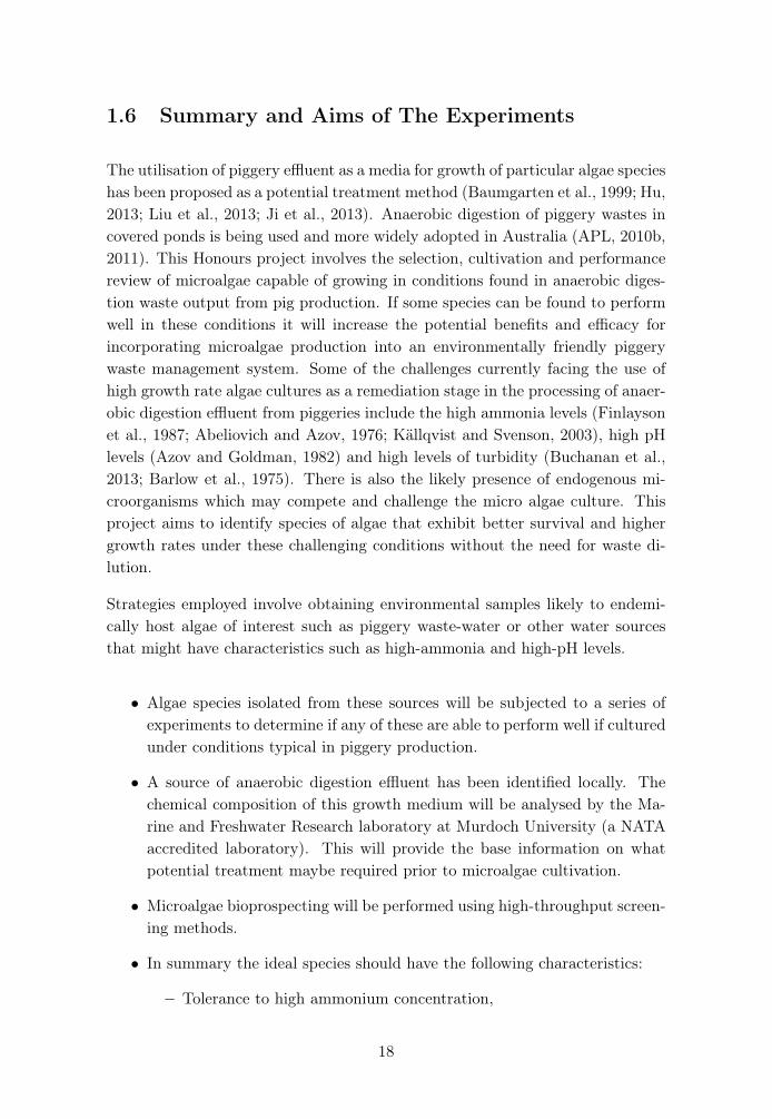
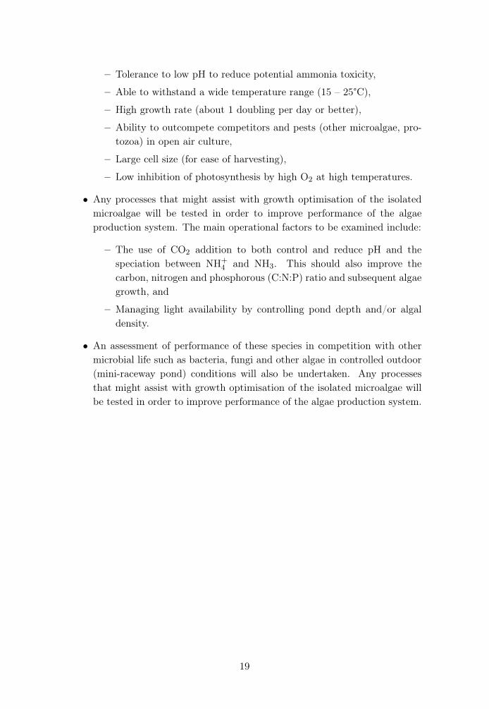
Two variations of internally illuminated photobioreactor designs are shown inFigure 1.12 and a pond design with CO2 addition is shown in Figure 1.13.

Figure 1.12: A schematic diagram of an internally illuminated photobioreactorilluminted by stationary light sources (left) (Ugwu et al., 2008) and a design conceptincorporating a rotating light array (right) (Teschler, 2009).

be modified in such a way that it can utilize both solar andartificial light system (Ogbonna et al., 1999). In that case,the artificial light source is switched on whenever the solarlight intensity decreases below a set value (during cloudyweather or at night). There are also some reports on theuse of optic fibers to collect and distribute solar light incylindrical photobioreactors (Mori, 1985; Matsunagaet al., 1991). One of the major advantages of internally-illu-minated photobioreactor is that it can be heat-sterilizedunder pressure and thus, contamination can be minimized.Furthermore, supply of light to the photobioreactor can bemaintained continuously (both day and night) by integrat-ing artificial and solar light devices. However, outdoormass cultivation of algae in this type of photobioreactorwould require some technical efforts.

3. Hydrodynamics and mass transfer characteristics ofphotobioreactors

Although relationship between hydrodynamics andmass transfer has been extensively investigated and corre-lated in bioreactors for heterotrophic cultures, only a fewstudies on these aspects are available in phototrophic cul-tures. Hydrodynamics and mass transfer characteristicsthat are applicable in photobioreactors include; the overallmass transfer coefficient (kLa), mixing, liquid velocity, gasbubble velocity and gas holdup.

The overall mass transfer coefficient (kLa) is the mostcommonly used parameters for assessing the performanceof photobioreactors. The term kLa is generally used todescribe the overall volumetric mass transfer coefficient inphotobioreactors. The volumetric mass transfer coefficient(kLa) of photobioreactors is dependent on various factorssuch as agitation rate, the type of sparger, surfactants/anti-foam agents and temperature.

Mixing time can be defined as the time taken to achievea homogenous mixture after injection of tracer solution.Lee and Bazin (1990) defines mixing time as the time takenfor a small volume of dye solution added to the liquid totransverse the reactor. Generally, mixing time is deter-mined in photobioreactors using tracer substances suchas dyes. However, mixing time can also be measured by sig-nal-response method using tracer and pH electrode (Cam-acho Rubio et al., 1999; Ugwu et al., 2003; Pruvost et al.,

2006). Furthermore, computational fluid dynamics (CFD)was used to evaluate global mixing in torus photobioreac-tor (Pruvost et al., 2006; Sato et al., 2006).

Mixing time is a very important parameter in designingphotobioreactors for various biological processes. Goodmixing would ensure high cell concentration, keep algalcells in suspension, eliminate thermal stratification, helpnutrient distribution, improve gas exchange as well asreduce the degree of mutual shading and lower the proba-bility of photoinhibition (Janvanmardian and Palsson,1991). It was also reported that when the nutritionalrequirements are sufficient and the environmental condi-tions are optimized, mixing aimed at inducing turbulentflow would result in high yield of algal biomass (Huet al., 1996). Bosca et al. (1991) demonstrated that the pro-ductivity of alga is higher in mixed culture than in anunmixed one under the same condition. Various mixingsystems are currently used in algal cultures depending onthe type of photobioreactors. In open pond systems, paddlewheels were used to induce turbulent flow (Boussiba et al.,1988; Hase et al., 2000). In stirred-tank photobioreactors,impellers were used in mixing algal cultures (Ogbonnaet al., 1999; Mazzuca Sobczuk et al., 2006). In tubular pho-tobioreactors, mixing can be done by bubbling air directlyor indirectly via airlift systems (Ogbonna and Tanaka,2001; Tredici and Chini Zittelli, 1998) or by installing staticmixers inside the tubes (Ugwu et al., 2002). Mixing systemsthat utilized baffles in bubble-column photobioreactorswere also demonstrated in algal cultures (Merchuk et al.,2000; Degen et al., 2001).

In bubble-column and large diameter tubular photobi-oreactors, demarcation exists between the light-illuminatedand dark surfaces. Thus mixing strategies should be intro-duced in cultures to circulate algal cells between the light-illuminated and dark regions of the photobioreactors(Molina Grima et al., 1999; Ugwu et al., 2005b; MazzucaSobczuk et al., 2006).

Increase in aeration rate would improve mixing, liquidcirculation, and mass transfer between gas and liquidphases in algal cultures. However, high aeration couldcause shear stress to algal cells (Mazzuca Sobczuk et al.,2006; Kaewpintong et al., 2007). Gas bubble velocity is ameasure of culture flow rates in tubular photobioreactors(plug flow regime) since algal cultures are circulated alongwith gas bubbles. When fine spargers are used to increasegas dispersion inside horizontal tubular photobioreactors,relatively large bubbles are produced. However, the bub-bles coalesce during flow to form interface between theliquid broth, gas and the walls of the tube. The contact areabetween the liquid and the gas is reduced, thereby, resultingto poor mass transfer rates.

Gas bubble velocity and size of the bubbles are depen-dent on the liquid flow rate. By increasing the gas flow rate,the bubble diameter increases, which consequently, wouldincrease the gas bubble velocity. The rate of gas circulationmay be interrupted when baffles or static mixers areinstalled inside the reactors to increase gas dispersion.

Impeller

Fluorescent lamp

Aeration port

Reactor wall

Rotor

Internally-illuminated photobioreactor

Fig. 1. Schematic diagram of an internally illuminated photobioreactor.

4024 C.U. Ugwu et al. / Bioresource Technology 99 (2008) 4021–4028

Figure 1.13: Side elevation of a high rate algal pond with CO2 addition to enhancealgal growth. (Park et al., 2010b).

2.1. Wastewater treatment HRAPs

Algae growing in wastewater treatment HRAPs assimilate nutri-ents and thus subsequent harvest of the algal biomass recovers thenutrients from the wastewater (García et al., 2006; Powell et al.,2009; Park and Craggs, 2010).

Wastewater treatment HRAPs are normally part of an AdvancedPond System which typically comprises advanced facultativeponds which incorporate anaerobic digestion pits, HRAP, algal set-tling ponds and maturation ponds in series (Craggs, 2005; Craggset al., in press). Based on design for BOD removal, Advanced PondSystems require approximately 50 times more land area than acti-vated sludge systems (one of the most common wastewater treat-ment technologies), although this does not account for the landarea needed to dispose of waste activated sludge. However, thecapital costs for construction of and Advanced Pond System areless than half and operational costs are less than one fifth thoseof activated sludge systems (Craggs et al., in press).

The simplest and most cost-effective option to convert algalbiomass to biofuel would be anaerobic digestion in an ambienttemperature covered digester pond to produce methane-rich bio-gas (Sialve et al., 2009; Craggs et al., in press), although moreexpensive heated and mixed anaerobic digesters could also beused. Biogas production rates from laboratory-scale ambient tem-perature covered digester ponds have been shown to be similar tothose of heated mixed digesters (0.21–0.28 m3 CH4/kg algal vola-tile solids (VS) added) (Sukias and Craggs, in press). Use of algalbiogas for electricity generation can produce approximately1 kWhelectricity/kg algal VS (Benemann and Oswald, 1996).

2.2. Economic and environmental advantages of biofuel productionfrom wastewater treatment HRAP

The comparisons between commercial algal production HRAPand wastewater treatment HRAP are summarized in Table 1. Thecosts of algal production and harvest using wastewater treatmentHRAP are essentially covered by the wastewater treatment plantcapital and operation costs and they have significantly less envi-ronmental impact in terms of water footprint, energy and fertiliseruse, and residual nutrient removal from spent growth mediumprior to discharge to avoid eutrophication of receiving waters.

Commercial algal farms require sources of water, nutrients andcarbon dioxide which contribute to 10–30% of total productioncosts (Borowitzka, 2005; Benemann, 2008a; Tampier, 2009; Cla-rens et al., 2010). Therefore, to minimize operational costs, com-mercial farms often recycle the growth medium following algalharvest (Borowitzka, 2005). However, growth medium re-use hasbeen implicated with reduced algal productivity due to increased

contamination by algal pathogens and/or accumulation of inhibi-tory secondary metabolites (Moheimani and Borowitzka, 2006).

While the demand for biofuel production is in part driven byenvironmental concerns, there is no doubt that building and oper-ating HRAP dedicated solely to produce algal biomass for biofuelhas an environmental impact in its own right. For example, freshwater resources are consumed via evaporation thus creating awater footprint. Indeed, Clarens et al. (2010) concluded that algalproduction using freshwater and fertilisers would consume moreenergy, have higher greenhouse gas emissions and use more waterthan biofuel production from land-based crops such as switch-grass, canola and corn.

Algal production from wastewater HRAPs by contrast offers afar more attractive proposition from an environmental viewpoint.The impacts of the HRAP construction and operation are a neces-sity of providing wastewater treatment and thus the subsequentalgal yield represents a biofuel feedstock free of this environmentalburden. Furthermore, the water and nutrients that are utilized inthese systems are neutral in that they are otherwise wasted. Theextraction of energy and subsequent application of the residual al-gal biomass to land represents a source of sustainable energy andfertiliser thus offering net environmental benefit. Moreover the useof HRAPs for wastewater treatment over other forms of wastewa-ter treatment can provide environment gains. For example, Shiltonet al. (2008) gave an example for a town of 25,000 people in theEnglish countryside where using a pond treatment option insteadof an electromechanical wastewater treatment system could save35 million kWh over a 30-year design life. They went onto notethat for the UK, where an average of 0.43 kg CO2 is emitted perkWh of electricity produced, this amounts to 500 tonnes of CO2

emitted per year which would require over 200 hectares of pineforest to soak up (Shilton et al., 2008).

While pond systems in general are one of the most commonforms of wastewater treatment technology used by small commu-nities around the world, to date the HRAP has not been as widelyapplied as facultative and maturation ponds which have providedsimple and reliable performance for many decades. However, withincreasing regulatory pressure to upgrade treatment for nutrientremoval and subsequent algal harvesting (Powell et al., in press)and with increasing recognition of the renewable energy produc-tion and potentially improved greenhouse gas management thatHRAPs offer, it is likely that they will become more widely appliedin the future.

3. Algal production

Many theoretical approaches to determine the maximum pho-tosynthetic solar energy conversion efficiency have been describedin the literature (for example, Weissman and Goebel, 1987; Tillett,

Wastewater influent

Gas flowmeter

CO2 addition sump (~1.5 m)

Effluent to algal harvester

Central baffle

Water flow

30-50 cm water depth

Paddle wheel

pH Sensor

CO2 addition controller

CO2 source

High Rate Algal Pond

Solenoid valve

Central dividingwall

Water flow

Fig. 1. Side elevation of a high rate algal pond with CO2 addition to enhance algal growth.

36 J.B.K. Park et al. / Bioresource Technology 102 (2011) 35–42

17

1.6 Summary and Aims of The Experiments

The utilisation of piggery effluent as a media for growth of particular algae specieshas been proposed as a potential treatment method (Baumgarten et al., 1999; Hu,2013; Liu et al., 2013; Ji et al., 2013). Anaerobic digestion of piggery wastes incovered ponds is being used and more widely adopted in Australia (APL, 2010b,2011). This Honours project involves the selection, cultivation and performancereview of microalgae capable of growing in conditions found in anaerobic diges-tion waste output from pig production. If some species can be found to performwell in these conditions it will increase the potential benefits and efficacy forincorporating microalgae production into an environmentally friendly piggerywaste management system. Some of the challenges currently facing the use ofhigh growth rate algae cultures as a remediation stage in the processing of anaer-obic digestion effluent from piggeries include the high ammonia levels (Finlaysonet al., 1987; Abeliovich and Azov, 1976; Källqvist and Svenson, 2003), high pHlevels (Azov and Goldman, 1982) and high levels of turbidity (Buchanan et al.,2013; Barlow et al., 1975). There is also the likely presence of endogenous mi-croorganisms which may compete and challenge the micro algae culture. Thisproject aims to identify species of algae that exhibit better survival and highergrowth rates under these challenging conditions without the need for waste di-lution.

Strategies employed involve obtaining environmental samples likely to endemi-cally host algae of interest such as piggery waste-water or other water sourcesthat might have characteristics such as high-ammonia and high-pH levels.

• Algae species isolated from these sources will be subjected to a series ofexperiments to determine if any of these are able to perform well if culturedunder conditions typical in piggery production.

• A source of anaerobic digestion effluent has been identified locally. Thechemical composition of this growth medium will be analysed by the Ma-rine and Freshwater Research laboratory at Murdoch University (a NATAaccredited laboratory). This will provide the base information on whatpotential treatment maybe required prior to microalgae cultivation.

• Microalgae bioprospecting will be performed using high-throughput screen-ing methods.

• In summary the ideal species should have the following characteristics:

– Tolerance to high ammonium concentration,

18

– Tolerance to low pH to reduce potential ammonia toxicity,

– Able to withstand a wide temperature range (15 – 25°C),

– High growth rate (about 1 doubling per day or better),

– Ability to outcompete competitors and pests (other microalgae, pro-tozoa) in open air culture,

– Large cell size (for ease of harvesting),

– Low inhibition of photosynthesis by high O2 at high temperatures.

• Any processes that might assist with growth optimisation of the isolatedmicroalgae will be tested in order to improve performance of the algaeproduction system. The main operational factors to be examined include:

– The use of CO2 addition to both control and reduce pH and thespeciation between NH+

4 and NH3. This should also improve thecarbon, nitrogen and phosphorous (C:N:P) ratio and subsequent algaegrowth, and

– Managing light availability by controlling pond depth and/or algaldensity.

• An assessment of performance of these species in competition with othermicrobial life such as bacteria, fungi and other algae in controlled outdoor(mini-raceway pond) conditions will also be undertaken. Any processesthat might assist with growth optimisation of the isolated microalgae willbe tested in order to improve performance of the algae production system.

19

Chapter 2

Materials and Methods

2.1 Chemicals and Solvents

Analytical grade (A.R.) chemicals were used throughout this study, with theexception of industrial grade Ammonium Chloride (NH4Cl). Analytical gradeacetone, neutralised with a small quantity of magnesium carbonate, was used fortotal chlorophyll extraction and analysis. Laboratory in-house deionised waterwas used in all procedures requiring the use of water.

2.2 Algal Culturing

2.2.1 Synthetic Media

Three synthetic media formulations were used during the bioprospecting andisolation phase of the experiment. One of these was a standard modified Chu-13media formulation based on the Botryococcus formula published in Chu (1942)(See Table 2.1). Two of these were variations of Chu-13 media using NH4Cl asthe nitrogen source in place of potassium nitrate (KNO3). Potassium hydroxide(KOH) was used to increase pH where required.

One of these variations known as Chu-55 for the experiment was made using210 mg.L�1 NH4Cl in order to match the 55mg of N provided in Chu-13 (SeeTable 2.2). The other variation used 1,909 mg.L�1 of NH4Cl in order to attain acloser match to the ammonia content of piggery effluent with 500 mg NH3-N.L�1

(See Table 2.3).

20

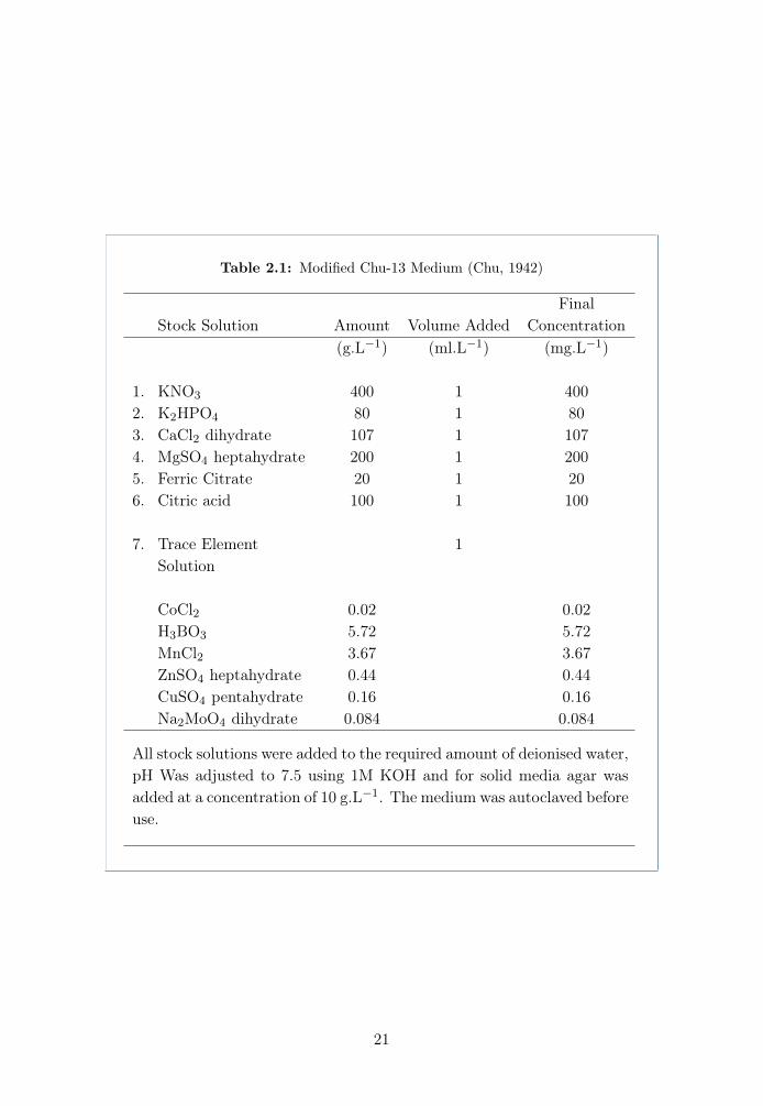
Table 2.1: Modified Chu-13 Medium (Chu, 1942)

FinalStock Solution Amount Volume Added Concentration

(g.L�1) (ml.L�1) (mg.L�1)

1. KNO3 400 1 4002. K2HPO4 80 1 803. CaCl2 dihydrate 107 1 1074. MgSO4 heptahydrate 200 1 2005. Ferric Citrate 20 1 206. Citric acid 100 1 100

7. Trace Element 1Solution

CoCl2 0.02 0.02H3BO3 5.72 5.72MnCl2 3.67 3.67ZnSO4 heptahydrate 0.44 0.44CuSO4 pentahydrate 0.16 0.16Na2MoO4 dihydrate 0.084 0.084

All stock solutions were added to the required amount of deionised water,pH Was adjusted to 7.5 using 1M KOH and for solid media agar wasadded at a concentration of 10 g.L�1. The medium was autoclaved beforeuse.

21

Table 2.2: Modified Chu-13 Medium (Chu, 1942) known as ‘Chu-55’.

FinalStock Solution Amount Volume Added Concentration

(g.L�1) (ml.L�1) (mg.L�1)

1. NH4Cl As Solid 2102. K2HPO4 80 1 803. CaCl2 dihydrate 107 1 1074. MgSO4 heptahydrate 200 1 2005. Ferric Citrate 20 1 206. Citric acid 100 1 100

7. Trace Element 1Solution

CoCl2 0.02 0.02H3BO3 5.72 5.72MnCl2 3.67 3.67ZnSO4 heptahydrate 0.44 0.44CuSO4 pentahydrate 0.16 0.16Na2MoO4 dihydrate 0.084 0.084

Stock solutions 2 to 8 were added to the required amount of deionisedwater, 10 g.L�1 agar added for solid media and autoclaved. For solidmedia after autoclaving media was left to cool and solidify on the benchovernight. Solid (after remelting) and liquid media were brought to 50°Cin a water bath before addition of NH4Cl in solid form and pH adjustedto 9 using autoclaved 1M KOH.

22

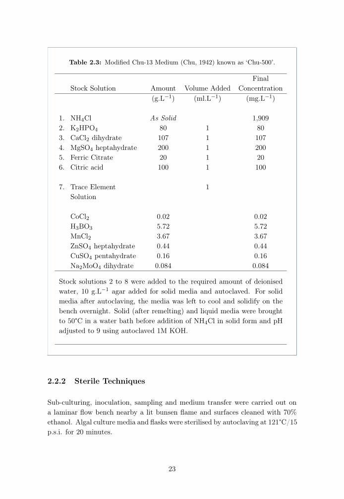
Table 2.3: Modified Chu-13 Medium (Chu, 1942) known as ‘Chu-500’.

FinalStock Solution Amount Volume Added Concentration

(g.L�1) (ml.L�1) (mg.L�1)

1. NH4Cl As Solid 1,9092. K2HPO4 80 1 803. CaCl2 dihydrate 107 1 1074. MgSO4 heptahydrate 200 1 2005. Ferric Citrate 20 1 206. Citric acid 100 1 100

7. Trace Element 1Solution

CoCl2 0.02 0.02H3BO3 5.72 5.72MnCl2 3.67 3.67ZnSO4 heptahydrate 0.44 0.44CuSO4 pentahydrate 0.16 0.16Na2MoO4 dihydrate 0.084 0.084

Stock solutions 2 to 8 were added to the required amount of deionisedwater, 10 g.L�1 agar added for solid media and autoclaved. For solidmedia after autoclaving, the media was left to cool and solidify on thebench overnight. Solid (after remelting) and liquid media were broughtto 50°C in a water bath before addition of NH4Cl in solid form and pHadjusted to 9 using autoclaved 1M KOH.

2.2.2 Sterile Techniques

Sub-culturing, inoculation, sampling and medium transfer were carried out ona laminar flow bench nearby a lit bunsen flame and surfaces cleaned with 70%ethanol. Algal culture media and flasks were sterilised by autoclaving at 121°C/15p.s.i. for 20 minutes.

23

2.2.3 Piggery anaerobic digestate based media

Piggery anaerobic digestate based media was sourced from the Medina ResearchStation at Kwinana south of Perth, WA. This research facility houses pigs in afarming environment. Effluent from the piggery is output into a covered anaer-obic digestion pond for biogas production (biogas is then flared off from thecovered pond intermittently as required). When this pond is filled to capacity,effluent exits to a secondary evaporation pond which is exposed to air, sunlightand rain.

The nutrient profile analysis of this material performed by the Marine and Fresh-water Research Laboratory is shown in Table 2.4. The ammonia nitrogen contentof this material was found to be 690 mg NH3-N.L�1 and the total phosphorouscontent was 43 mg P.L�1. Dissolved organic carbon was measured at 97 mgC.L�1 and the total organic carbon was 220 mg C.L�1. The pH of the anaerobicdigestion effluent was 7.41 for unfiltered, 8.23 for charcoal filtered and 7.95 forsand filtered (At the time of measurement 1 sample was available for each of theunfiltered and charcoal filtered and three samples were measured and averagedfor the sand filtered effluent).

Anaerobic digestion effluent used for algae isolation was pumped directly fromthe covered anaerobic digestion pond and stored in 30L capacity plastic drums.Early in the project, pig production had been inactive for a period of roughlyone month due to maintenance at the piggery and the pond at this time did notappear to be actively producing biogas (See Table 2.4). Later in the project,some pigs were housed at the piggery. However, due to cleaning operations atthe piggery, large volumes of water were washed through the anaerobic digestionpond giving a lower nutrient load (See Table 2.5).

For the initial bioprospecting phase of the experiment, anaerobic digestion ef-fluent was filtered through charcoal before use in algae cultures. Some algaecultures were attempted with raw unfiltered effluent however, culture perfor-mance was found to be inferior when compared to filtered effluent and thus allsubsequent effluent was filtered through charcoal or sand. For use in the racewaypond, effluent was filtered through a sand filter that was made at the lab.

In the raceway ponds, anaerobic digestion effluent was enriched with NH4Cl tosustain experimental conditions of 800, 1000, 1200 and 1600 mg NH3-N.L�1 andpH adjusted to 9 using KOH pellets.

24

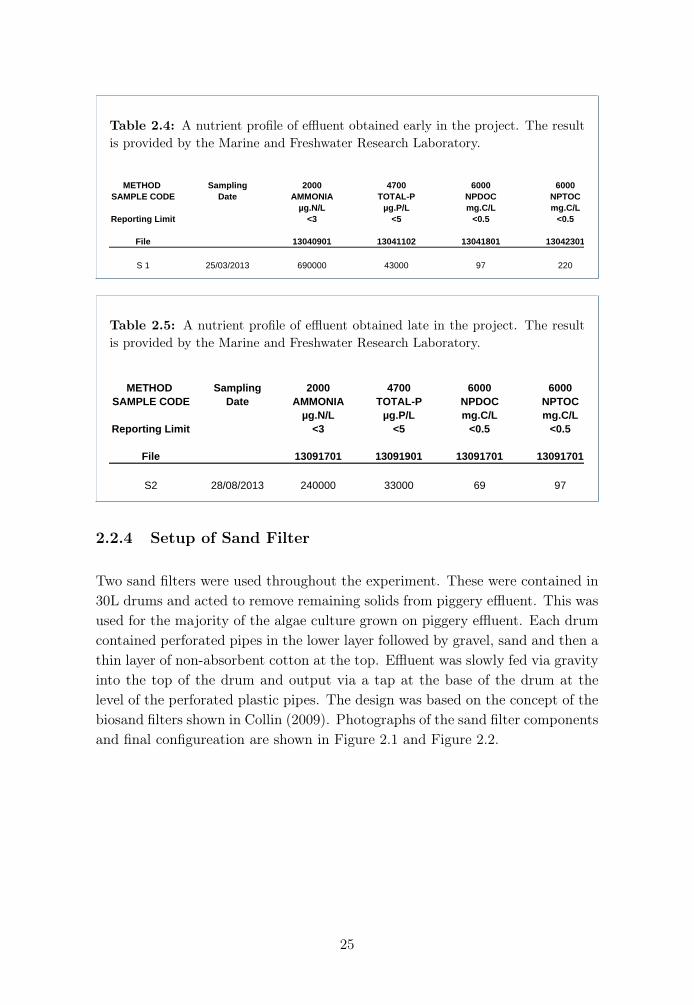
Table 2.4: A nutrient profile of effluent obtained early in the project. The resultis provided by the Marine and Freshwater Research Laboratory.

Contact: Jeremy Ayre Date of Issue: 30/04/2013Customer: Biological Sciences Date Received: 28/03/2013Address: Murdoch University, 90 South Street, Murdoch 6150 Our Reference: BSB13-2

METHOD Sampling 2000 4700 6000 6000SAMPLE CODE Date AMMONIA TOTAL-P NPDOC NPTOC

µg.N/L µg.P/L mg.C/L mg.C/LReporting Limit <3 <5 <0.5 <0.5

File 13040901 13041102 13041801 13042301

S 1 25/03/2013 690000 43000 97 220

WATER QUALITY DATA

Signatory:

Date: 30/04/2013

All test items tested as received. Spare test items will be held for two months unless otherwise requested.

This document may not be reproduced except in full. Page 1 of 1

Table 2.5: A nutrient profile of effluent obtained late in the project. The resultis provided by the Marine and Freshwater Research Laboratory.

Contact: Jeremy Ayre Date of Issue: 24/09/2013Customer: Algae Research Laboratory, School of Veterinary and Life Sciences Date Received: 16/09/2013Address: Murdoch University, 90 South St, Murdoch, 6150 Our Reference: BSB13-9

METHOD Sampling 2000 4700 6000 6000SAMPLE CODE Date AMMONIA TOTAL-P NPDOC NPTOC

µg.N/L µg.P/L mg.C/L mg.C/LReporting Limit <3 <5 <0.5 <0.5

File 13091701 13091901 13091701 13091701

S2 28/08/2013 240000 33000 69 97

WATER QUALITY DATA

Signatory:

Date: 24/09/2013

All test items tested as received. Spare test items will be held for two months unless otherwise requested.

This document may not be reproduced except in full. Page 1 of 1

2.2.4 Setup of Sand Filter

Two sand filters were used throughout the experiment. These were contained in30L drums and acted to remove remaining solids from piggery effluent. This wasused for the majority of the algae culture grown on piggery effluent. Each drumcontained perforated pipes in the lower layer followed by gravel, sand and then athin layer of non-absorbent cotton at the top. Effluent was slowly fed via gravityinto the top of the drum and output via a tap at the base of the drum at thelevel of the perforated plastic pipes. The design was based on the concept of thebiosand filters shown in Collin (2009). Photographs of the sand filter componentsand final configureation are shown in Figure 2.1 and Figure 2.2.

25

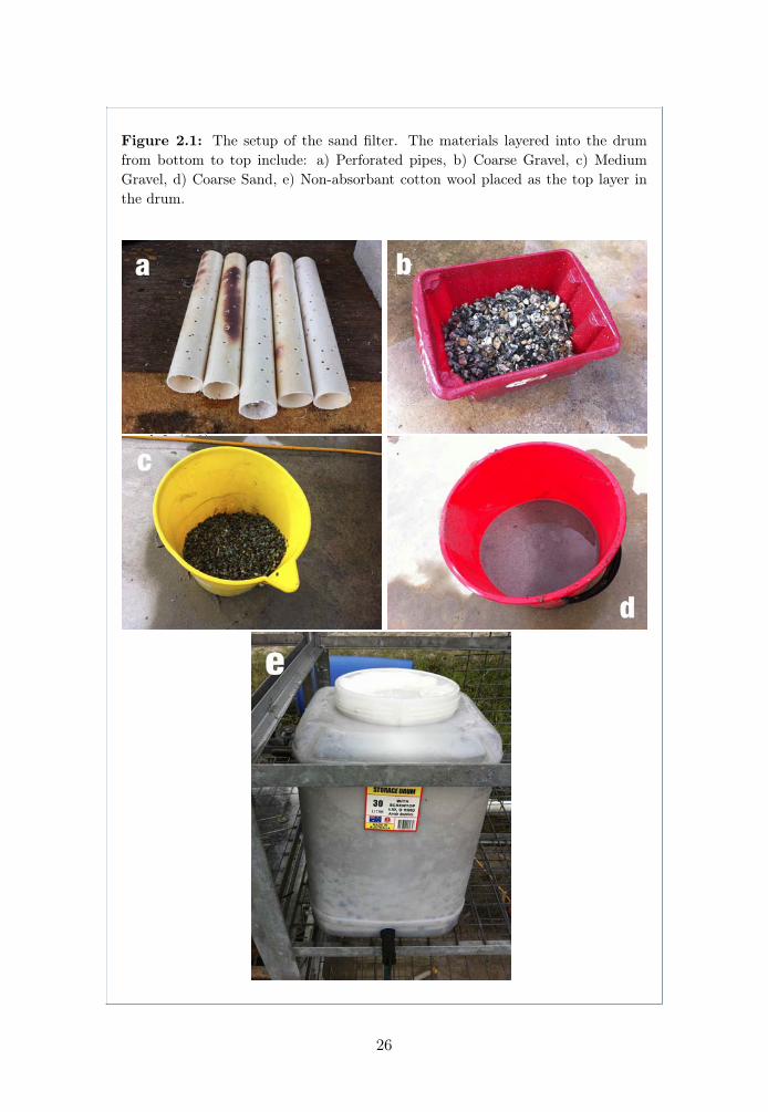
Figure 2.1: The setup of the sand filter. The materials layered into the drumfrom bottom to top include: a) Perforated pipes, b) Coarse Gravel, c) MediumGravel, d) Coarse Sand, e) Non-absorbant cotton wool placed as the top layer inthe drum.

top left (0,0)

26

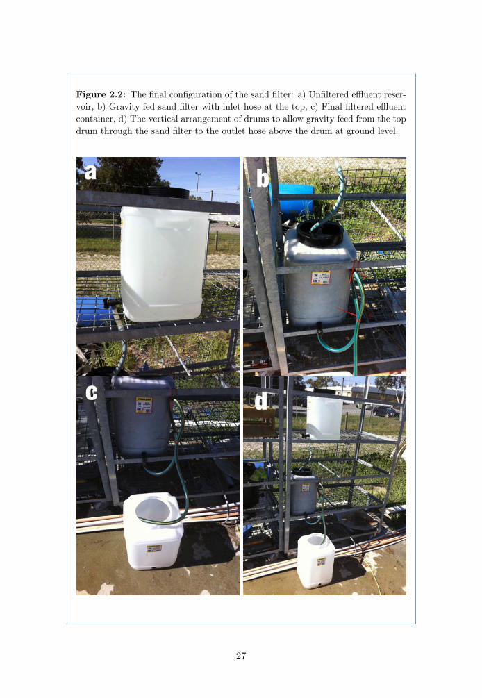
Figure 2.2: The final configuration of the sand filter: a) Unfiltered effluent reser-voir, b) Gravity fed sand filter with inlet hose at the top, c) Final filtered effluentcontainer, d) The vertical arrangement of drums to allow gravity feed from the topdrum through the sand filter to the outlet hose above the drum at ground level.

27

2.3 Analytical Methods

2.3.1 Nutrient Characterisation

Effluent samples were delivered to the Marine and Freshwater Research Lab-oratory at Murdoch University and analysed for Ammonia, Total Phosphate,Dissolved Organic Carbon and Total Organic Carbon.

Methods performed were as outlined in APHA (2012):

• Ammonia: ‘APHA 4500-NH3 H - Phenate/Flow injection’,

• Total-P: ‘APHA 4500-P B, 4500-P G Persulphate/ Flow injection’,

• NPDOC (Non-Purgeable Dissolved Organic Carbon): ‘APHA 5310 B HighTemperature combustion method, Infrared Detection’, and

• NPTOC (Non-Purgeable Total Organic Carbon): ‘APHA 5310 B HighTemperature combustion method, Infrared Detection’.

2.3.2 Biomass

Biomass as total dry weight were determined as follows:

Whatman GF/C (2.5cm diameter) filters were placed in an oven for 1 hour at 100°C. Filters were then placed in a vacuum desiccator and stored over KOH pelletsuntil use. Filters were weighed to 5 decimal places on an analytical balance.Weighed filters were then placed into a Millipore filter apparatus and 5 mL ofalgal culture drained through using vacuum suction until the filters appeared dry.Filters were then folded and placed into an oven for 1 hour at 100 °C before beingstored overnight in a vacuum desiccator over KOH pellets. After the overnightinterval, dried filters were again weighed to 5 decimal places. Dry weight wascalculated as the weight of the original filter subtracted from the total weight offilter with algae sample deposition.

To determine ash free dry weight, filter samples were placed in a furnace at 450°C for 5 hours. Filters were then placed again into a vacuum desiccator over KOHpellets to cool overnight. Filters were then weighed to 5 decimal places and theoriginal filter weight subtracted from the final remaining weight to obtain theweight of ash. The ash weight was subtracted from the dry weight to obtain theash free dry weight. The AFDW value divided for a 5 mL sample can thereforebe given as: the resulting weight/0.005 in mg.L�1

28

2.3.3 Chlorophyll determination

Chlorophyll extraction and measurement calculations were performed as followsusing the protocol outlined in Jeffrey and Humphrey (1975):

Whatman GF/C (2.5cm diameter) filters were placed into a Millipore filter appa-ratus and 5 mL of algal culture drained through using vacuum suction until thefilters appeared dry. Filter paper samples were then folded and enclosed withinaluminium foil in order to shield samples from light and placed in a freezer forpreservation until chlorophyll extraction was performed.

Chlorophyll extraction was performed using analytical grade acetone at 90%concentration with 10% DI water and a pinch of magnesium carbonate to removeany acid present.

The solvent was stored on ice during the extraction with all extraction workperformed under low light.

A glass rod was used to grind filter samples in a glass test tube with 4mL of thesolvent in total to extract algal pigments. Once liquified, samples were placedinto 10mL centrifuge tubes. Samples were then centrifuged for 10 minutes andthe supernatant removed for analysis by spectrophotometer.

Absorbance readings were performed and recorded at 630, 647 and 664 nm wave-lengths.

Quantification of chlorophyll a, b and c was calculated as per the equationspublished in Jeffrey and Humphrey (1975).

2.3.4 Cell Count

A 5 mL sample of the algae culture was immobilised with 200 µL of Lugol’siodine. Samples were refrigerated for up to 3 days until cell-count performed.Prior to counting sample was gently homogenised in a glass tissue grinder witha loose fitting teflon plunger. Cell numbers were determined using a Neubauerhaemocytometer and a Leitz Laborlux 12 microscope.

For the most dominant cell type a minimum of 100 cells were counted in orderto achieve 5-10% coefficient of variation for each determination. For less dom-inant cell types a count was performed for 400 of the smallest squares on thehaemocytometer equivalent to one of the large size squares or a volume of 0.1µL.

29

2.3.5 Ammonia determination

Ammonia concentration in pond, effluent and algae culture samples was per-formed using a Hanna Instruments ‘HI 733’ Model ammonia test kit.

2.3.6 Temperature

Temperature measurements in outdoor raceway ponds were determined with 2x YSI 6-Series Sondes and 2 x Tinytag data recorders. Some temperature datawas also downloaded from the Murdoch University ‘On-line Weather Station’ athttp://wwwmet.murdoch.edu.au.

2.3.7 pH

In the laboratory, pH was determined with standard pH probe and battery orAC powered pH meter. In the outdoor raceway ponds pH was determined using2 x YSI 6-Series Sondes. For pH adjustments of synthetic media 1M KOH wasused. For raceway ponds, KOH pellets were added directly to the raceway pondsto simulate high pH piggery effluent. In raceway ponds where CO2 was beingadded pH stat units connected to electronic solenoid valves allowed gas entrydirectly into the pond water until the pH dropped to between 7.9 and 8.

2.4 Isolation of Algae Strains

2.4.1 Sources of Samples

Various water and soil samples were obtained from sources believed likely toharbour potentially useful algae strains as part of the bioprospecting strategy.These were selected based on environmental conditions likely to favour ammoniatolerance, extreme pH variation and other characteristics that might be associ-ated with algae that have been exposed to or able to survive in piggery effluent.Tolerance to extreme variation in temperature and moisture levels were also con-sidered useful for the algae of interest. Convenience of collection location wasalso important in order to obtain samples early in the isolation stage of theexperiment.

The primary sources of algae utilised early in the experiment included:

30

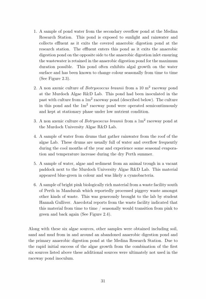
1. A sample of pond water from the secondary overflow pond at the MedinaResearch Station. This pond is exposed to sunlight and rainwater andcollects effluent as it exits the covered anaerobic digestion pond at theresearch station. The effluent enters this pond as it exits the anaerobicdigestion pond on the opposite side to the anaerobic digestion inlet ensuringthe wastewater is retained in the anaerobic digestion pond for the maximumduration possible. This pond often exhibits algal growth on the watersurface and has been known to change colour seasonally from time to time(See Figure 2.3).

2. A non axenic culture of Botryococcus braunii from a 10 m2 raceway pondat the Murdoch Algae R&D Lab. This pond had been inoculated in thepast with culture from a 1m2 raceway pond (described below). The culturein this pond and the 1m2 raceway pond were operated semicontinuouslyand kept at stationary phase under low nutrient condition.

3. A non axenic culture of Botryococcus braunii from a 1m2 raceway pond atthe Murdoch University Algae R&D Lab.

4. A sample of water from drums that gather rainwater from the roof of thealgae Lab. These drums are usually full of water and overflow frequentlyduring the cool months of the year and experience some seasonal evapora-tion and temperature increase during the dry Perth summer.

5. A sample of water, algae and sediment from an animal trough in a vacantpaddock next to the Murdoch University Algae R&D Lab. This materialappeared blue-green in colour and was likely a cyanobacteria.

6. A sample of bright pink biologically rich material from a waste facility southof Perth in Mandurah which reportedly processed piggery waste amongstother kinds of waste. This was generously brought to the lab by studentHannah Gulliver. Anecdotal reports from the waste facility indicated thatthis material from time to time / seasonally would transition from pink togreen and back again (See Figure 2.4).

Along with these six algae sources, other samples were obtained including soil,sand and mud from in and around an abandoned anaerobic digestion pond andthe primary anaerobic digestion pond at the Medina Research Station. Due tothe rapid initial success of the algae growth from the combination of the firstsix sources listed above these additional sources were ultimately not used in theraceway pond inoculum.

31

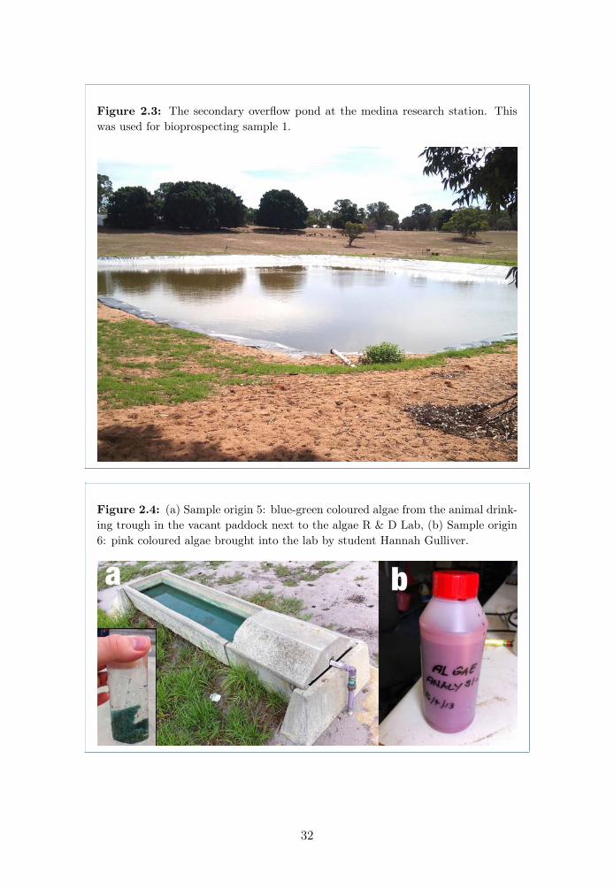
Figure 2.3: The secondary overflow pond at the medina research station. Thiswas used for bioprospecting sample 1.

Figure 2.4: (a) Sample origin 5: blue-green coloured algae from the animal drink-ing trough in the vacant paddock next to the algae R & D Lab, (b) Sample origin6: pink coloured algae brought into the lab by student Hannah Gulliver.

32

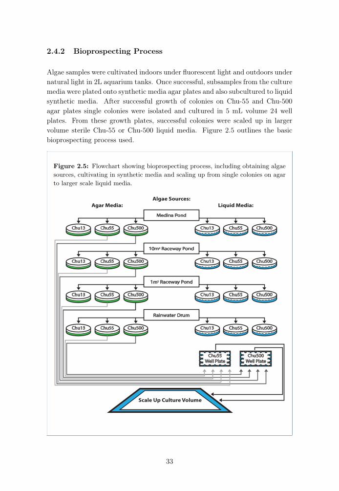
2.4.2 Bioprospecting Process

Algae samples were cultivated indoors under fluorescent light and outdoors undernatural light in 2L aquarium tanks. Once successful, subsamples from the culturemedia were plated onto synthetic media agar plates and also subcultured to liquidsynthetic media. After successful growth of colonies on Chu-55 and Chu-500agar plates single colonies were isolated and cultured in 5 mL volume 24 wellplates. From these growth plates, successful colonies were scaled up in largervolume sterile Chu-55 or Chu-500 liquid media. Figure 2.5 outlines the basicbioprospecting process used.

Figure 2.5: Flowchart showing bioprospecting process, including obtaining algaesources, cultivating in synthetic media and scaling up from single colonies on agarto larger scale liquid media.

Algae Sources:Agar Media: Liquid Media:

Chu55Well Plate

Medina Pond

Chu500Chu55Chu13 Chu13 Chu55 Chu500

10m2 Raceway Pond

Chu500Chu55Chu13 Chu13 Chu55 Chu500

1m2 Raceway Pond

Chu500Chu55Chu13 Chu13 Chu55 Chu500

Rainwater Drum

Chu500Chu55Chu13 Chu13 Chu55 Chu500

Chu500Well Plate

Scale Up Culture Volume

33

2.4.3 Bioprospecting Culture Tanks

The four initial sources of inoculum were cultivated indoors, one set of four usingcharcoal filtered effluent as growth media and the other set of four using unfilteredeffluent as growth media. Culture vessels used were small aquarium tanks witha 2L capacity. Into these were placed approximately 200mL of inoculum. In thecase of inoculum source 1, approximately 50mL of the sample was made up to200mL with tap water. Each inoculum had 800mL of the filtered or unfilteredpiggery effluent added bringing each total volume to 1L. The 1L point was markedon the side of each tank so that any evaporation of water could be compensatedfor with fresh tapwater as required during the algae culture growth.

Each tank was aerated using an ‘airstone’ attached to plastic piping originatingfrom an aquarium air pump. Tanks were illuminated with fluorescent lampsrunning vertically alongside at a distance of roughly 10 - 20cm from the tankwalls. Light measurement was performed around the indoor growth tanks andfound to be 400-440 µmol photons m�2s�1 on the side of the tank closest to thelight. On the side of the tank away from the light (being blocked by the growthmedia) light measurements were taken for the filtered effluent and unfilteredeffluent and found to be 60 and 6 µmol photons m�2s�1 respectively.

The indoor tanks were subject to a 12 hour light cycle with light on during theday from 7am to 7pm. The culture room was temperature controlled to 25 °C.

34

Figure 2.6: Indoor culture vessels. The top vessel contains filtered effluent. Thelower vessels contains unfiltered effluent. Photographs were taken immediatelyafter culture setup and inoculum (first day of the isolation phase). The colourdifference between filtered and unfiltered effluent is quite noticeable.

An additional four culture vessels were setup on an outdoor bench near thenorth facing wall of the lab sheltered under the eaves of the building. Identical2L aquarium growth vessels were used with an airstone in each culture media asdescribed above. The same inoculum sources were used in each of these tanks asdescribed above however 500mL volumes were used. 500mL volumes of filteredeffluent were used to make each culture media up to 1L in volume.

An additional large outdoor aquarium tank (approximately 40 x 60 cm horizontaldimensions and 30cm depth) was also setup with 4L of effluent and 40mL ofinoculum from each of the smaller outdoor tanks. An ‘air-curtain’ aeration devicewas placed in this tank. The effluent media volume in this tank was raised to8L and then 16L during the course of the experiment as successful algae growthwas observed.

Light measurements around the outdoor tanks were found to be 200-215 µmolphotons m�2s�1 in the ambient light under the shade of the building eaves.During the afternoon from approximately 4.50pm to 6pm, direct sunlight reachedthe outdoor tank. Light in the direct sun in front of the tank was measured at 700µmol photons m�2s�1. Behind the tank sunlight levels were measured at 9 µmolphotons m�2s�1. As well as being subject to variable light levels temperaturelevels were quite variable reaching up to 39 °C measured during the daytime in

35

early April (the start of the bioprospecting phase) and up to 47 °C measuredduring the daytime in early May when the outdoor area was exposed to a longerperiod of direct sunlight (due to the position against a north facing wall of thebuilding). The outdoor area fell to 12 °C overnight minimum in May and 2 °Covernight minimum in June.

36

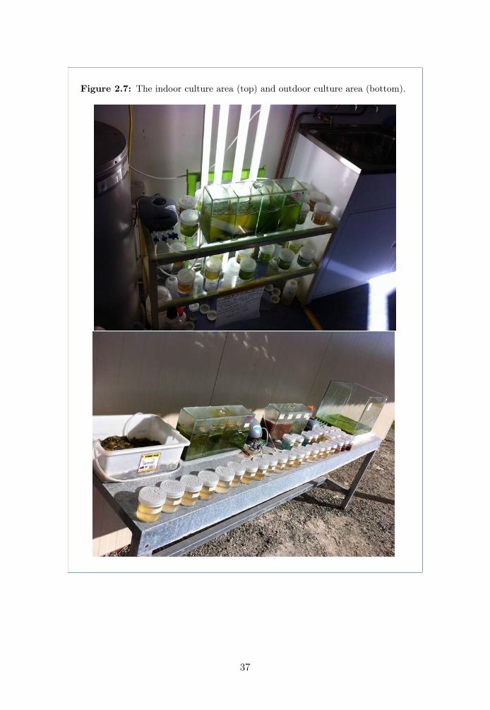
Figure 2.7: The indoor culture area (top) and outdoor culture area (bottom).

37

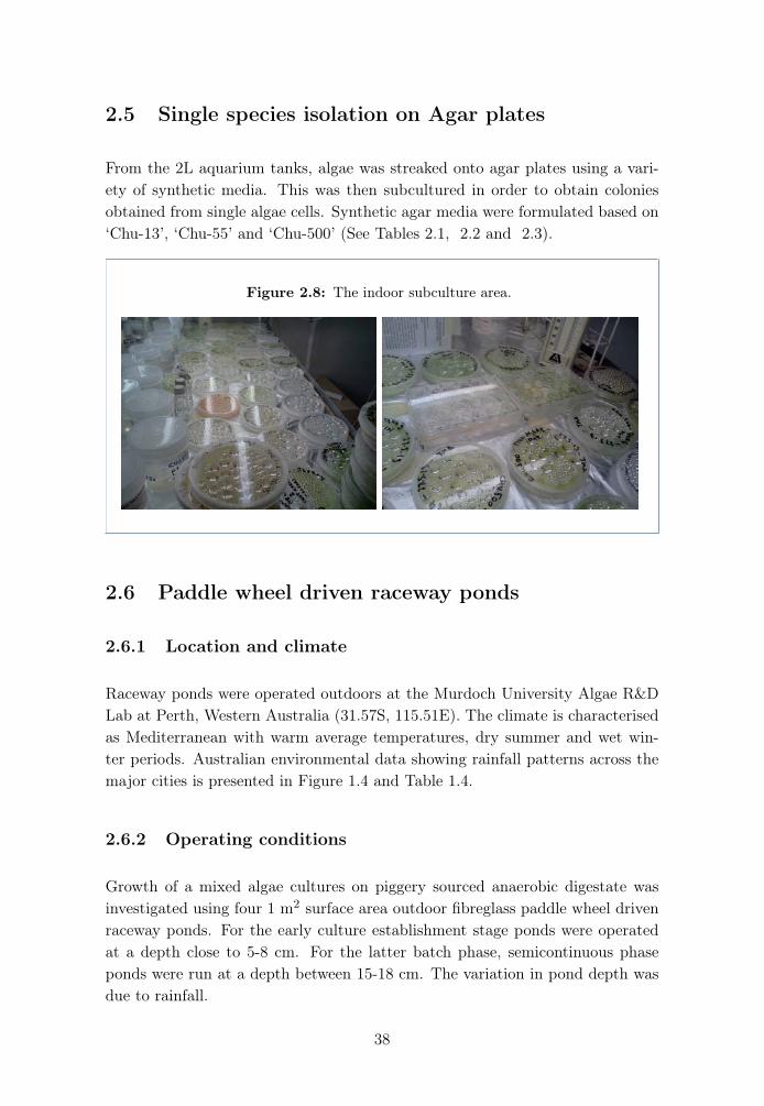
2.5 Single species isolation on Agar plates

From the 2L aquarium tanks, algae was streaked onto agar plates using a vari-ety of synthetic media. This was then subcultured in order to obtain coloniesobtained from single algae cells. Synthetic agar media were formulated based on‘Chu-13’, ‘Chu-55’ and ‘Chu-500’ (See Tables 2.1, 2.2 and 2.3).

Figure 2.8: The indoor subculture area.

2.6 Paddle wheel driven raceway ponds

2.6.1 Location and climate

Raceway ponds were operated outdoors at the Murdoch University Algae R&DLab at Perth, Western Australia (31.57S, 115.51E). The climate is characterisedas Mediterranean with warm average temperatures, dry summer and wet win-ter periods. Australian environmental data showing rainfall patterns across themajor cities is presented in Figure 1.4 and Table 1.4.

2.6.2 Operating conditions

Growth of a mixed algae cultures on piggery sourced anaerobic digestate wasinvestigated using four 1 m2 surface area outdoor fibreglass paddle wheel drivenraceway ponds. For the early culture establishment stage ponds were operatedat a depth close to 5-8 cm. For the latter batch phase, semicontinuous phaseponds were run at a depth between 15-18 cm. The variation in pond depth wasdue to rainfall.

38

Figure 2.9: Raceway pond (1 m2) (a) photograph including charcoal filteredeffluent with inoculum (b) schematic diagram of raceway pond (adapted from Mo-heimani (2005)).

For investigating the effect of dif trations on growth, pH was kept

constant by a CO2-stat system troller and a solenoid switch

connected to a CO gas cylinder. pH was logged using a DataTaker DT 50 data logger.

A floating CO trap/injector based on the design of Becker (1994) with 0.06 m2 surface

area was used to maximise CO2 transfer into the liquid phase (Figure 20). The pond

temperature was recorded continuously using an underwater Tiny Tag TG-3110

temperature logger. Air temperature, irradiance and humidity data were obtained from

the Murdoch University weather station. The average photosynthetic active radiation

(PAR, 400-700nm) received by the pond was calculated by the Equation 10, where

0.429 is the fraction of PAR in the solar spectrum (Thimijan and Henis 1983).

Light penetration into the culture media was measured using an under water light sensor

at different cell concentrations.

ferent CO2 concen

using a Roche 8001 pH con

2

2

PAR = [Average daily irridiance (W.m-2)] x (1m2)x (0.429) Eq. 10

Figure 19. Raceway pond (1 m2) (a) photograph (b) schematic diagram of raceway pond.

One of the ponds was kept as a control during the experiments. Experiments on various

levels of pH (adding known volume of CO2), photosynthetic adaptation, optimum

79

2.6.3 Culture establishment phase

In order to establish a viable culture with tolerance to high ammonia and highpH conditions, a single pond (labelled pond 4) was operated for a period ofseveral weeks from its initial setup on the 17th of April 2013. A 15L volume ofcharcoal filtered effluent was added to the pond with a 3.5L inoculum containinga mixture of 500L volumes from all bioprospecting aquarium tanks which wereat that stage exhibiting strong algae growth. This inoculum included tanks 1and 2 (indoors) differing from tanks 1, 2, 3 and 4 (outdoors) and an additional500mL of algae sample from the secondary effluent pond at Medina ResearchStation.

The following day after initial setup another 30L of charcoal filtered effluent wasadded to this pond bringing the volume to roughly 48.5L. A further 5L was addedon the 29th of April and 30th of April with 1.5L added on the 1st May to bringthe total pond volume to 60L.

On May 2 a second raceway pond (labelled pond 3) was established using 27Lof sand filtered effluent and 3L inoculum from the first pond. An additional30L piggery effluent was added to this pond the following day bringing the totalvolume to 60L. On the 21st of May a CO2 controller was setup and tested inpond 3 with CO2 being pumped into the pond until the pH dropped from 7.5-8.

39

On June 4 an additional 2 raceway ponds (labelled 1 and 2) were setup to preparefor a total of 4 ponds operating simultaneously. Pond 1 was left as a control withno inoculum and pond 2 was inoculated with 100mL from each of the four indoortanks, and 6 outdoor tanks and made up the remainder of the 6L volume withinoculum from pond 3.

From the 5th of June regular ammonia measurements were performed acrossall four raceway ponds while the ammonia level of pond 3 and 4 was graduallyraised from 5th of June to 21st of June to above 800mg NH3-N.L�1 with regularadditions of NH4Cl (66.8g added each time). Ponds 1 and 2 did not have anyNH4Cl added.

2.6.4 Batch and semicontinuous phase with high ammonia andCO2 addition

On the 5th of July, in order to prepare for the next experiment phase, media werehomogenised across all ponds by removing 3 x 20L volumes from each pond anddistributing these across alternate ponds. This process was performed twice toensure sufficient mixing. To enrich the pond cultures, a 1L volume of algae wasadded to each pond from the large outdoor aquarium which had been exposed toextreme temperature variations from around 2 - 39 °C during the winter months.

NH4Cl was added to each of the ponds to bring the N level up to 800 mg NH3-N.L�1. On the following day the pH of each of the ponds was adjusted to 9 usingKOH pellets. From the 6th of July to 9th of July the ponds were operated withno further NH4Cl or KOH addition.

From the 10th of July two of the ponds were raised to 1000 mg NH3-N.L�1 whiletwo remained at 800 mg NH3-N.L�1. One of the 800 and one of the 1000 weresubjected to CO2 addition until the pH dropped below 8. Pond 2 and 4 wereagain raised in ammonia level to 1200 mg NH3-N.L�1 after 1.5 weeks, and 1600mg NH3-N.L�1 after another 1.5 weeks.

From the 19th of August for a period of 5 weeks a semicontinuous growth phasewas operated for all four ponds. Figure 2.10 shows the details of the time periodsoperated for the raceway ponds.

40

Figure 2.10: Timeline showing the different stages of the experiment which involved the use of the 1m2 outdoor raceway ponds.

17#April)>

1#May2#May#)>#4#July 5#June#)>#9#July

10#July)>

21#July

22#July)>

1#August

2#August)>

18#August19#August#)>#25#September

(2#Weeks) (4.5#Weeks) (5#Weeks) (1.5#Weeks)

(1.5#Weeks)

(2#Weeks) (5#Weeks)

Semicontinuous#Phase

Pond#1: 500#)>#0#mg#NH3)N#L)1

(Measure(NH3(loss(with(no(inoculum)800#mg#NH3)N#L

)1 Pond#1:

Pond#2: 500#)>#0#mg#NH3)N#L)1

(Measure(NH3(loss(with(inoculum(added)

1000#mg#

NH3)N#L)1

1200#mg#

NH3)N#L)1

1600#mg#NH3)

N#L)11600#mg#NH3)N#L

)1 Pond#2:

Pond#3: Approx#590#)>#0#mg#NH3)N#L)1 Approx#130#)>#800#mg#NH3)N#L

)1

(Addition(of(66.8(g(NH4Cl(every(3(days)800#mg#NH3)N#L

)1#+CO2 Pond#3:

Pond#4:Approx#690#mg#NH3)N#L)1#

Continuation#)>#0#mg#NH3)N#L)1 Approx#130#)>#800#mg#NH3)N#L

)1

(Addition(of(66.8(g(NH4Cl(every(3(days)

1000#mg#

NH3)N#L)1#

+CO2

1200#mg#

NH3)N#L)1#

+CO2

1600#mg

NH3)N#L)1#

+CO2

1600#mg#NH3)N#L)1#+CO2 Pond#4:

Batch#Phase

800#mg#NH3)N#L)1

800#mg#NH3)N#L)1#+CO2

Bioprospecting#Phase

41

Chapter 3

Microalgae bioprospecting

3.1 Introduction

The majority of studies involving the treatment of piggery anaerobic digestionwastewater with algae have focused on algae culture using diluted wastewatermedia with reduced ammonium content (Chung et al., 1978; Chiu et al., 1980;Fallowfield and Garrett, 1985; Strain et al., 1986; Hu, 2013). Under Australianconditions water is a scarce resource. Australia is the worlds driest continent afterAntarctica with average rainfall of below 600 mm for over 80% of the continentand below 300 mm for more than 50% (Pink, 2012). Although a piggery in anAustralian context may utilise the capture of rainwater in tanks or dams andflush fresh or recycled water into it’s wastewater treatment through the actionof washing and cleaning the piggery, the addition of fresh water to the piggerywaste treatment system would generally be considered an unaffordable luxury.

For this reason, the main focus of this study was to find species of microalgaecapable of growing in undiluted anaerobic digestion piggery wastewater effluent.The bioprospecting strategy employed has focused on obtaining one or more algalspecies which are capable of growing in undiluted anaerobic digestion wastewater.As the current trend in Australian piggeries is to incorporate anaerobic digestionas a primary wastewater treatment, undiluted anaerobic digestate is the idealtarget effluent for algae culture.

The nutrient profile of anaerobic digestion effluent from a piggery is likely to varyconsiderably over time and geographic location. However, certain characteristicsappear to be typical such as high pH, high ammonia concentration and highturbidity. As all autotrophic or mixotrophic species either require or are greatly

42

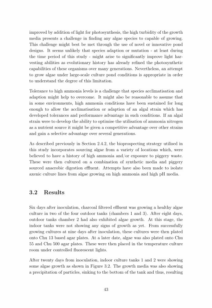
improved by addition of light for photosynthesis, the high turbidity of the growthmedia presents a challenge in finding any algae species to capable of growing.This challenge might best be met through the use of novel or innovative ponddesigns. It seems unlikely that species adaption or mutation - at least duringthe time period of this study - might arise to significantly improve light har-vesting abilities as evolutionary history has already refined the photosyntheticcapabilities of these organisms over many generations. Nevertheless, an attemptto grow algae under large-scale culture pond conditions is appropriate in orderto understand the degree of this limitation.

Tolerance to high ammonia levels is a challenge that species acclimatisation andadaption might help to overcome. It might also be reasonable to assume thatin some environments, high ammonia conditions have been sustained for longenough to allow the acclimatisation or adaption of an algal strain which hasdeveloped tolerances and performance advantage in such conditions. If an algalstrain were to develop the ability to optimise the utilisation of ammonia nitrogenas a nutrient source it might be given a competitive advantage over other strainsand gain a selective advantage over several generations.

As described previously in Section 2.4.2, the bioprospecting strategy utilised inthis study incorporates sourcing algae from a variety of locations which, werebelieved to have a history of high ammonia and/or exposure to piggery waste.These were then cultured on a combination of synthetic media and piggerysourced anaerobic digestion effluent. Attempts have also been made to isolateaxenic culture lines from algae growing on high ammonia and high pH media.

3.2 Results

Six days after inoculation, charcoal filtered effluent was growing a healthy algaeculture in two of the four outdoor tanks (chambers 1 and 3). After eight days,outdoor tanks chamber 2 had also exhibited algae growth. At this stage, theindoor tanks were not showing any signs of growth as yet. From successfullygrowing cultures at nine days after inoculation, these cultures were then platedonto Chu 13 based agar plates. At a later date, algae was also plated onto Chu55 and Chu 500 agar plates. These were then placed in the temperature cultureroom under controlled fluorescent lights.

After twenty days from inoculation, indoor culture tanks 1 and 2 were showingsome algae growth as shown in Figure 3.2. The growth media was also showinga precipitation of particles, sinking to the bottom of the tank and thus, resulting

43

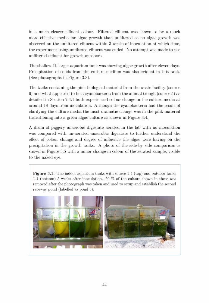
in a much clearer effluent colour. Filtered effluent was shown to be a muchmore effective media for algae growth than unfiltered as no algae growth wasobserved on the unfiltered effluent within 3 weeks of inoculation at which time,the experiment using unfiltered effluent was ended. No attempt was made to useunfiltered effluent for growth outdoors.

The shallow 4L larger aquarium tank was showing algae growth after eleven days.Precipitation of solids from the culture medium was also evident in this tank.(See photographs in Figure 3.3).

The tanks containing the pink biological material from the waste facility (source6) and what appeared to be a cyanobacteria from the animal trough (source 5) asdetailed in Section 2.4.1 both experienced colour change in the culture media ataround 18 days from inoculation. Although the cyanobacteria had the result ofclarifying the culture media the most dramatic change was in the pink materialtransitioning into a green algae culture as shown in Figure 3.4.

A drum of piggery anaerobic digestate aerated in the lab with no inoculationwas compared with un-aerated anaerobic digeatate to further understand theeffect of colour change and degree of influence the algae were having on theprecipitation in the growth tanks. A photo of the side-by side comparison isshown in Figure 3.5 with a minor change in colour of the aerated sample, visibleto the naked eye.

Figure 3.1: The indoor aquarium tanks with source 1-4 (top) and outdoor tanks1-4 (bottom) 5 weeks after inoculation. 50 % of the culture shown in these wasremoved after the photograph was taken and used to setup and establish the secondraceway pond (labelled as pond 3).

44

Figure 3.2: The indoor aquarium tanks at 20 days after inoculation. In all tankssolids can be seen settling out of the pond media. Algae growth is noticeable inthe second chamber of the filtered effluent.

Figure 3.3: The large outdoor aquarium with 4 L volume of algae culture shownat 11 days after inoculation.

45

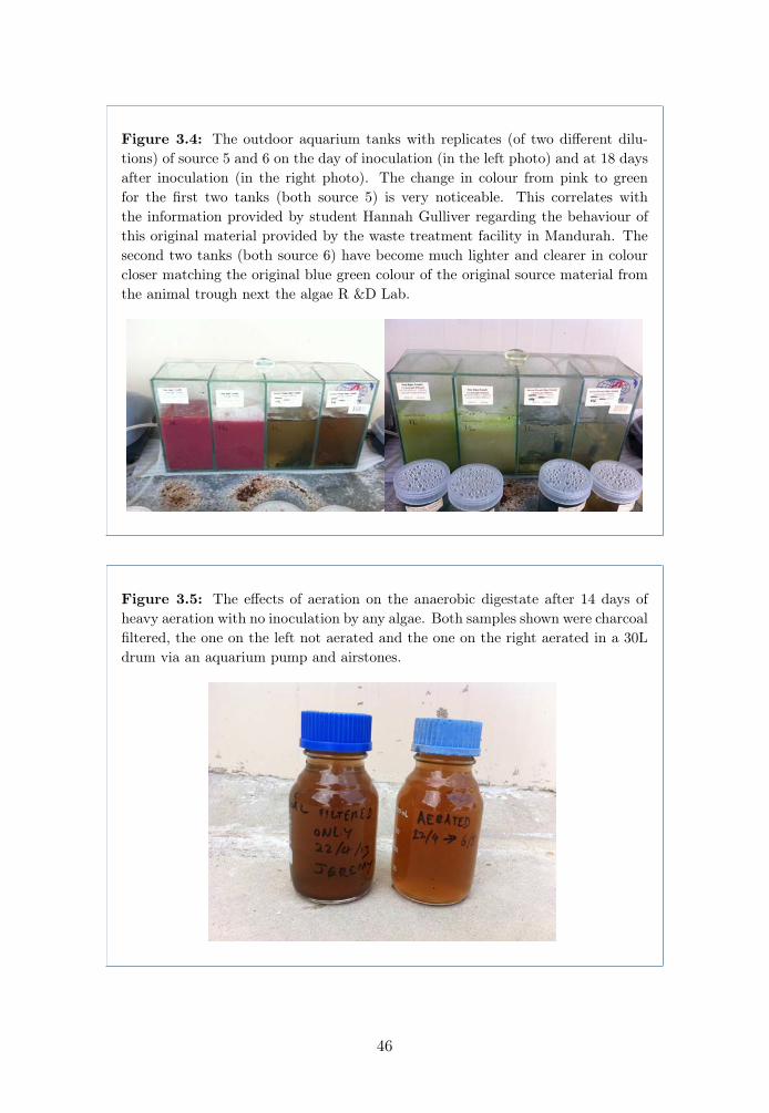
Figure 3.4: The outdoor aquarium tanks with replicates (of two different dilu-tions) of source 5 and 6 on the day of inoculation (in the left photo) and at 18 daysafter inoculation (in the right photo). The change in colour from pink to greenfor the first two tanks (both source 5) is very noticeable. This correlates withthe information provided by student Hannah Gulliver regarding the behaviour ofthis original material provided by the waste treatment facility in Mandurah. Thesecond two tanks (both source 6) have become much lighter and clearer in colourcloser matching the original blue green colour of the original source material fromthe animal trough next the algae R &D Lab.

Figure 3.5: The effects of aeration on the anaerobic digestate after 14 days ofheavy aeration with no inoculation by any algae. Both samples shown were charcoalfiltered, the one on the left not aerated and the one on the right aerated in a 30Ldrum via an aquarium pump and airstones.

46

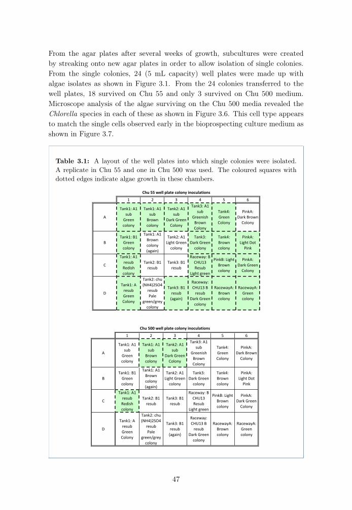
From the agar plates after several weeks of growth, subcultures were createdby streaking onto new agar plates in order to allow isolation of single colonies.From the single colonies, 24 (5 mL capacity) well plates were made up withalgae isolates as shown in Figure 3.1. From the 24 colonies transferred to thewell plates, 18 survived on Chu 55 and only 3 survived on Chu 500 medium.Microscope analysis of the algae surviving on the Chu 500 media revealed theChlorella species in each of these as shown in Figure 3.6. This cell type appearsto match the single cells observed early in the bioprospecting culture medium asshown in Figure 3.7.

Table 3.1: A layout of the well plates into which single colonies were isolated.A replicate in Chu 55 and one in Chu 500 was used. The coloured squares withdotted edges indicate algae growth in these chambers.

1 2 3 4 5 6

A

Tank1:-A1-sub

Green-colony

Tank1:-A1-sub

Brown-colony

Tank2:-A1-sub

Dark-Green-Colony

Tank3:-A1-sub

Greenish-Brown-Colony

Tank4:-Green-Colony

PinkA:Dark-Brown-Colony

BTank1:-B1Green-colony

Tank1:-A1Brown-colony-(again)

Tank2:-A1Light-Green-colony

Tank3:Dark-Green-colony

Tank4:Brown-colony

PinkA:Light-Dot-Pink

C

Tank1:-A1-resubRedish-colony

Tank2:-B1-resub

Tank3:-B1-resub

Raceway:-B-CHU13-Resub

Light-green

PinkB:-Light-Brown-colony

PinkA:Dark-Green-Colony

D

Tank1:-A-resubGreen-Colony

Tank2:-chu-(NH4)2SO4-

resubPale-

green/grey-colony

Tank3:-B1-resub(again)

Raceway:-CHU13-B-resub

Dark-Green-colony

RacewayA:Brown-colony

RacewayA:Green-colony

Chu$55$well$plate$colony$inoculations

1 2 3 4 5 6

A

Tank1:-A1-sub

Green-colony

Tank1:-A1-sub

Brown-colony

Tank2:-A1-sub

Dark-Green-Colony

Tank3:-A1-sub

Greenish-Brown-Colony

Tank4:-Green-Colony

PinkA:Dark-Brown-Colony

BTank1:-B1Green-colony

Tank1:-A1Brown-colony-(again)

Tank2:-A1Light-Green-colony

Tank3:Dark-Green-colony

Tank4:Brown-colony

PinkA:Light-Dot-Pink

C

Tank1:-A1-resubRedish-colony

Tank2:-B1-resub

Tank3:-B1-resub

Raceway:-B-CHU13-Resub

Light-green

PinkB:-Light-Brown-colony

PinkA:Dark-Green-Colony

D

Tank1:-A-resubGreen-Colony

Tank2:-chu-(NH4)2SO4-

resubPale-

green/grey-colony

Tank3:-B1-resub(again)

Raceway:-CHU13-B-resub

Dark-Green-colony

RacewayA:Brown-colony

RacewayA:Green-colony

Chu$500$well$plate$colony$inoculations

47

Figure 3.6: A photo of the dominant Chlorella species. This was the most com-mon species counted in cell counts throughout the study. It was observed frequentlyin both single cell and multicellular forms. Multicellular clumps such as shown inthis picture were not uncommon, even though efforts were made to homogenisesamples and disperse clumping prior to cell counting (Photo taken 20th of Septem-ber).

Figure 3.7: Early bioprospecting tank 3 indoors also showed the dominantChlorella (Photo taken 13th May).

48

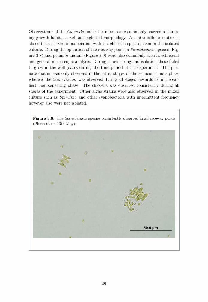
Observations of the Chlorella under the microscope commonly showed a clump-ing growth habit, as well as single-cell morphology. An intra-cellular matrix isalso often observed in association with the chlorella species, even in the isolatedculture. During the operation of the raceway ponds a Scenedesmus species (Fig-ure 3.8) and pennate diatom (Figure 3.9) were also commonly seen in cell countand general microscopic analysis. During subculturing and isolation these failedto grow in the well plates during the time period of the experiment. The pen-nate diatom was only observed in the latter stages of the semicontinuous phasewhereas the Scenedesmus was observed during all stages onwards from the ear-liest bioprospecting phase. The chlorella was observed consistently during allstages of the experiment. Other algae strains were also observed in the mixedculture such as Spirulina and other cyanobacteria with intermittent frequencyhowever also were not isolated.

Figure 3.8: The Scenedesmus species consistently observed in all raceway ponds(Photo taken 13th May).

49

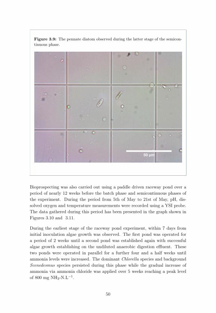
Figure 3.9: The pennate diatom observed during the latter stage of the semicon-tinuous phase.

Bioprospecting was also carried out using a paddle driven raceway pond over aperiod of nearly 12 weeks before the batch phase and semicontinuous phases ofthe experiment. During the period from 5th of May to 21st of May, pH, dis-solved oxygen and temperature measurements were recorded using a YSI probe.The data gathered during this period has been presented in the graph shown inFigures 3.10 and 3.11.

During the earliest stage of the raceway pond experiment, within 7 days frominitial inoculation algae growth was observed. The first pond was operated fora period of 2 weeks until a second pond was established again with successfulalgae growth establishing on the undiluted anaerobic digestion effluent. Thesetwo ponds were operated in parallel for a further four and a half weeks untilammonia levels were increased. The dominant Chlorella species and backgroundScenedesmus species persisted during this phase while the gradual increase ofammonia via ammonia chloride was applied over 5 weeks reaching a peak levelof 800 mg NH3-N.L�1.

50

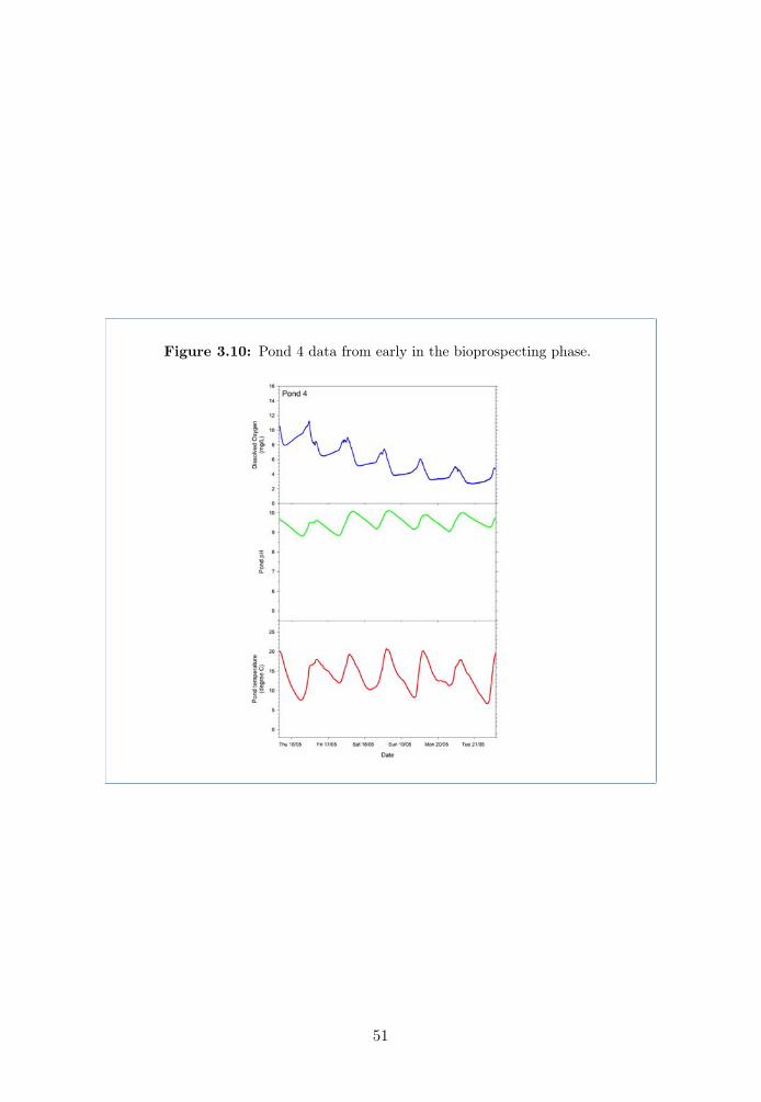
Figure 3.10: Pond 4 data from early in the bioprospecting phase.

51

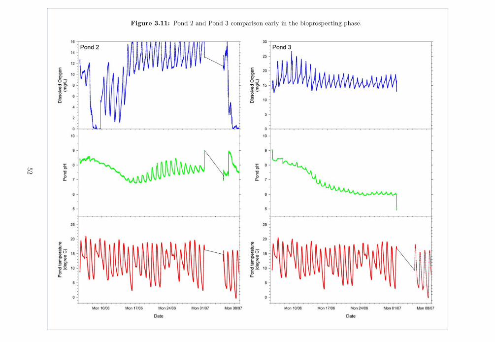
Figure 3.11: Pond 2 and Pond 3 comparison early in the bioprospecting phase.

52

3.3 Discussion

The outcome of this bioprospecting study indicates the successful cultivation ofalgae species capable of growing at a high ammonium content on undiluted pig-gery anaerobic digestate effluent. It is the author’s understanding that this isthe first time that this has been reported. Up to now, studies in the literatureindicated no algae growth at this combination of high pH and high ammonialevels. Hu (2013) recently reports being able to isolate Chlorella and Hindakiaspecies which were grown at small scale using several treatments of piggery ma-nure including anaerobic digestion and medium dilution and other studies reportalgae growth on ammonia levels up to approximately 500 mg NH3-N.L�1 (Bar-low et al., 1975; Fallowfield and Garrett, 1985; Kebede-Westhead et al., 2006;de Godos et al., 2010). Aguirre et al. (2011) reports on the use of piggery wastewith 790 mg NH3-N.L�1 being used for a mixed algae culture however an elec-troflocculation pretreatment method was employed. No reports are known ofraceway pond scale culture growth and isolation of species shown to grow inthe range at or above 800 mg NH3-N.L�1 using untreated anaerobic digestionpiggery effluent as found in this study.

The isolation of the chlorella strain on a synthetic media with at up to 500 mgNH3-N.L�1 is also encouraging and indicative of potential to grow an axenic cul-ture if further experiments were to follow on a time frame beyond the scope ofthis project. A similar method of acclimatisation and subculturing used in thisproject over a longer time would no doubt increase the statistical probability ofisolating different more diverse species and strains. The unexpected and spon-taneous appearance of the pennate diatom in the raceway ponds toward the endof the experiment is testament to the role that chance plays. This species ap-peared outside the bioprospecting stage of the experiment and appeared capableof survival even at 1,600 mg NH3-N.L�1.

Another interesting observation during this stage of the experiment was the ef-fect of aeration and algae growth on the precipitation and colour improvement inthe algae culture. Aeration alone was found to offer some improvement in the ef-fluent colour for both inoculated and un-inoculated anaerobic digestate, howeverthe strongest colour improvement was observed with strong algae growth. Thisappears to support the hypothesis that the turbidity is partially due to phospho-rous content in the wastewater, the action of bacteria (anaerobic or aerobic) andalgae utilising this phosphorous which has the effect of removing the turbidityresulting in cleaner water appearance (Ong et al., 2006).

Observations of the change in pH and dissolved oxygen during the early bio-

53

prospecting phase in pond 4 show a small increase in pH of the pond media asthe culture grew and a consistently high pH of between 9 and 10. Dissolved oxy-gen levels decreased steadily over time. This may have been due to a decrease inoxygen output from the algae as the growth slowed and nutrient depletion beganto limit photosynthesis.

During the period from 5th of June through to 9th of July the pH of pond 3can be seen steadily decreasing due to the addition of ammonium chloride tothe pond water. This indicates the need for addition of potassium hydroxideduring the batch and semicontinuous phases in order to compensate for the pHchange as the ammonium chloride is added. Pond 2 can also be seen during thistime with a steadily fluctuating pattern of pH change remaining consistent atan average just above 7 indicating a healthy culture with good photosyntheticactivity corresponding to daily temperature and dissolved oxygen fluctuations.

Early on in this experiment it was found that algae growth could not be supportedon unfiltered effluent, however in both aquarium tanks and the raceway pondscharcoal or sand filtration enabled the subsequent growth of algae under normallighting conditions. Once sand filtration was established as an effective method,charcoal filtration was abandoned in favour of sand filtration as this was believedto be much more economically viable and relevant for use in a full scale piggerysystem.

The Chlorella isolated and grown successfully on Chu 500 media appears mor-phologically identical to the dominant strain observed in the raceway pondsthroughout the duration of the study. During analysis chlorophyll a and b werefound at significant levels, however little or no chlorophyll c was detected. Thisclearly indicates the domination of green algae species (i.e. Chlorophyta) overother groups of algae which contain Chlorophyll c such as Haptophyta and Bacil-lariophyta.

54

Chapter 4

Reliable long term outdoor

cultivation

4.1 Introduction

Algae growth using diluted or pre-treated piggery waste has been reported instudies published over several decades (Barlow et al., 1975; Fallowfield and Gar-rett, 1985; Kebede-Westhead et al., 2006; de Godos et al., 2010; Aguirre et al.,2011; Hu, 2013). However, examples of large scale microalgae culture on un-treated, undiluted piggery wastewater appear to be rare or absent from theliterature. A range of wastewater treatments may be useful prior to microalgaeculture, however this study has focused on utilising undiluted anaerobic diges-tion effluent in it’s untreated form with only basic sand filtration. This algaemedia has been selected in an attempt to present a microalgae culture optionthat can be developed further for use in a full-scale piggery system. Due tothe increasing use of anaerobic digestion ponds by many Australian piggeriesand limitation on water supplies under Australian conditions these constraintsseem reasonable and fitting with the goal of developing a useful technology forpiggeries (Buchanan et al., 2013).

Leading on from the earlier bioprospecting phase of the project in which four ho-mogenous raceway pond cultures were established, several experiments were per-formed operating the ponds in parallel with identical configurations apart fromthe experimental variables being tested. The variables investigated throughoutthe study were different levels of ammonia, high pH and the addition of CO2 asa pH stabiliser.

55

An initial batch phase culture was operated for a 5 week period investigatingculture performance with sustained ammonia nitrogen levels between 800 andincreasing up to 1600 mg NH3-N.L�1. Duplicate ponds at identical ammonialevels were operated with the addition of CO2.

Following on from the batch phase a semicontinuous phase was established acrossall four raceway ponds. During this phase two ponds were operated at 800 mgNH3-N.L�1 and two were operated at 1600 mg NH3-N.L�1. One of each of the800 and 1600 variants was operated with addition of CO2 while the other wasoperated with no CO2 addition. Figure 2.10 outlines the timeline of the pondconditions.

4.2 Results

Data obtained from the Murdoch university weather station for the experimentalperiod is shown in Figure 4.1. At the start of large-scale culture in the racewayponds during mid July this is some of the coolest and wettest weather conditionsof the year. Overnight temperatures dropped to single digits while daytimetemperatures remained steadily in the low 20s. Solar radiation is also at the lowpart of the yearly cycle with roughly half the watts per square metre observedduring the warmer months. Rainfall is also it’s highest point in the year with 4to 8 ml of rain recorded on several days during July and August.

56

Figure 4.1: Graph of Murdoch University weather station environmental data. Data shown includes solar radiation, rain fall andtemperature (dew point, soil temperature at 250mm and air temperature). Period shown is from start of March to end of Octobercovering the period experiments were performed in the raceway ponds (17th of April to 3rd of October).

57

4.2.1 Natural ammonia decrease in raceway ponds

Prior to the establishment of the batch phase culture during the end of thebioprospecting phase two ponds were operated with identical volumes and con-ditions, however one was inoculated with algae while the other served as a controlwith no inoculation. A total of 6L inoculum was used in a total pond volume of85L. The aim of this experiment was to measure the change in ammonia levelsbetween the two ponds and establish a background level of ammonia uptake byalgae vs ammonia uptake without algae. The ammonia measurements performedduring this stage of the experiment are shown in Figure 4.2.

Figure 4.2: Measurements of ammonia levels in an inoculated pond (pond 2) anda control with no inoculation (pond 1).

58

Ammonia levels are observed decreasing across both ponds at a similar ratereaching close to zero ammonia measurable by the end of a two week period.Interestingly algae growth was observed at nearly identical levels in both theinoculated and control ponds.

4.2.2 Batch phase growth

Batch phase cultures were operated from the 10th of July to the 18th of August.During this time ponds labelled 1 and 3 were operated at 800 mg NH3-N.L�1

with regular measurements and top-up of ammonium chloride. Pond 3 also hadthe addition of CO2. During this time ponds labelled 2 and 4 were operated with1,000 mg NH3-N.L�1 from 10th July to 21st July (approx. 1.5 weeks), 1,200 mgNH3-N.L�1 from 22nd July to 1st August (approx. 1.5 weeks) and 1,600 mgNH3-N.L�1 from 2nd August to 18th August. Pond 4 also had the addition ofCO2.

Data obtained during this phase of the experiment is shown on the followingpages. Figure 4.3 shows ammonia measurement and top-up data, Figures 4.4and 4.5 show pH, dissolved oxygen and temperature data, Figure 4.6 cell counts,Figure 4.7 ash-free-dry-weight and Figure 4.8 chlorophyll extraction data.

Ammonia levels across the ponds as seen in Figure 4.3 during the batch phasetended to drop quite quickly down close to about 600 mg NH3-N.L�1 over ap-proximately two days in the case of the 800 mg NH3-N.L�1 ponds. The higherlevel pond has a similar relative drop off down from 1,200 to 1,000 and downfrom 1,600 to 1,400 mg NH3-N.L�1. Additions of ammonium chloride to theponds three times a week maintained a relatively steady ammonium nitrogencontent for most of the period with occasional fluctuations observed. A drop inammonia concentration in late July and again around the 9th of August cor-relates with rainfall around these times diluting the pond water. No obviouschange in ammonia levels is seen due to the addition of CO2 to ponds 3 and 4with the ammonia fluctuation patterns appearing relatively similar between theponds with the same top up treatment levels.

Dissolved oxygen levels in the ponds along with the pH data set in Figures 4.4and 4.5 show a more distinct difference between the ponds with CO2 additioncompared with the ponds with atmospheric CO2. The CO2 addition appears tobring the dissolved oxygen levels down much further than the comparison pondswith no CO2 addition. The pH levels can be seen responding to the forcedaddition of the CO2 gas into the pond water with a quicker pH drop off afterthe spike of ammonia and KOH is added to the pond pushing the pH back to

59

9. Ultimately however even the pH of the ponds without CO2 addition doessteadily drop down to match the base level prior to the top up of ammonia andKOH. The data shows a tendency for all of the ponds to stabilise back down toa pH of just below 7 during the time periods observed.

Cell counts observed as reported in Figure 4.6 show an initial drop in cell numbersearly in the batch phase but a relatively stable cell count overall across the fiveweeks. Drops in cell count appear to follow a similar pattern the dilution effect ofthe rainfall observed in the ammonia concentrations. Toward the end of the batchphase cell counts appear to be increasing again indicating cell growth in a highervolume of pond water due to the rainfall events through the period. Variation incell numbers across all four ponds and experimental conditions appears relativelysmall, however pond 4 with the final ammonia level of 1,600 mg NH3-N.L�1 andCO2 addition appears to maintain and finish the period with the highest Chlorellacell count between the four ponds.

Ash free dry weight data presented in Figure 4.7 shows a similar pattern to cellcount and ammonia data with minor fluctuations likely rainfall related. Pond 4again appears to perform above the others with the highest figures and a steadyrise toward the end of the period.

Chlorophyll data as seen in Figure 4.8 shows possibly the most significant dif-ference in the data with a clear advantage for ponds 3 and 4. Ponds 3 and 4appear overall to trend toward a gradual rise in chlorophyll a and b levels whereasponds 1 and 2 are quite steady with perhaps a small decline. The chlorophyll c1+ c2 data for all ponds appears very close to zero with little indication of anysignificant amounts of chlorophylls c1 or c2.

60

Figure 4.3: All ponds batch phase ammonia measurements and top-up levels.

61

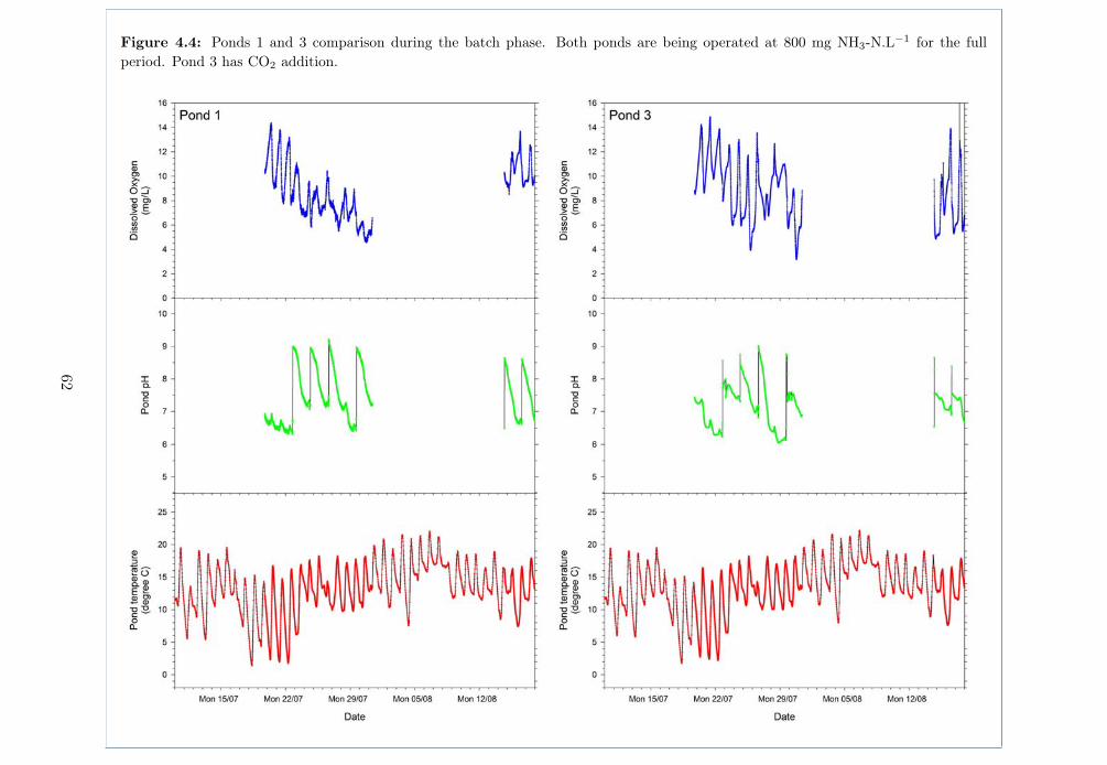
Figure 4.4: Ponds 1 and 3 comparison during the batch phase. Both ponds are being operated at 800 mg NH3-N.L�1 for the fullperiod. Pond 3 has CO2 addition.

62

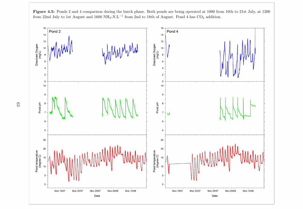
Figure 4.5: Ponds 2 and 4 comparison during the batch phase. Both ponds are being operated at 1000 from 10th to 21st July, at 1200from 22nd July to 1st August and 1600 NH3-N.L�1 from 2nd to 18th of August. Pond 4 has CO2 addition.

63

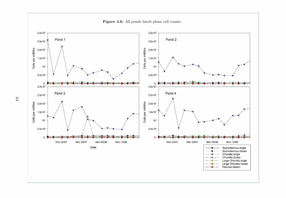
Figure 4.6: All ponds batch phase cell counts.

64

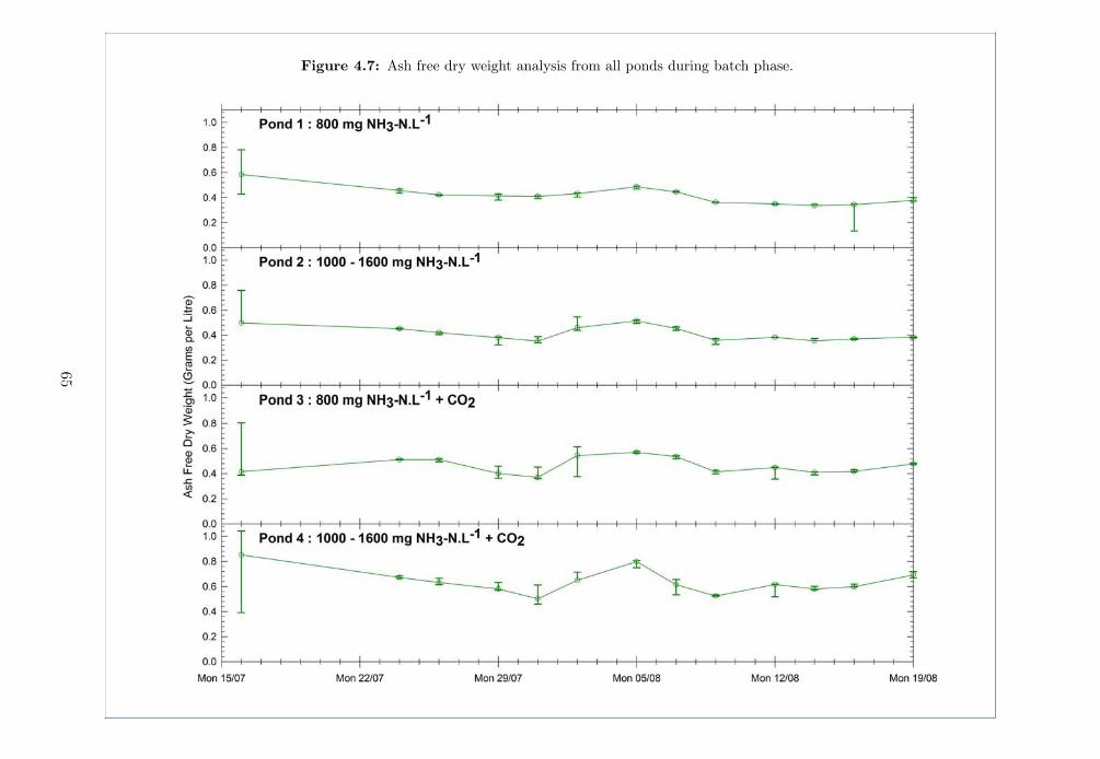
Figure 4.7: Ash free dry weight analysis from all ponds during batch phase.

65

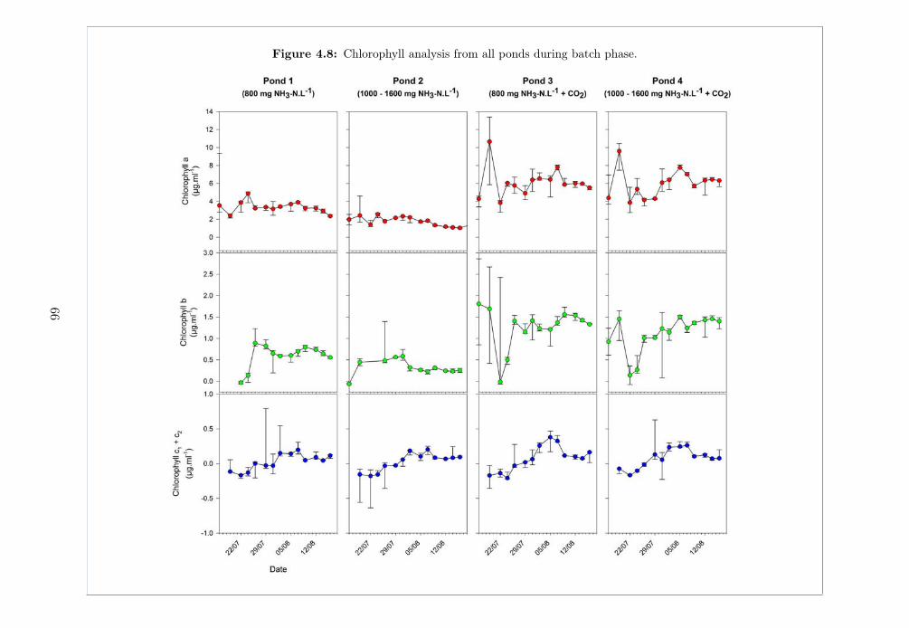
Figure 4.8: Chlorophyll analysis from all ponds during batch phase.

66

4.2.3 Semicontinuous phase

Semicontinuous phase cultures were operated from the 19th of August to the25th of September. During this time ponds labelled 1 and 3 were maintained at800 mg NH3-N.L�1. CO2 additions to pond 3 was continued as they were duringthe batch phase. During this time ponds 2 and 4 were maintained at 1600 mgNH3-N.L�1. CO2 additions to pond 4 were also continued as during the batchphase.

Data obtained during this final phase of the experiment are shown on the follow-ing pages. Figure 4.9 shows ammonia measurement and top-up data, Figure 4.10and 4.11 shows pH, dissolved oxygen and temperature data, Figure 4.12 cellcounts, Figure 4.13 ash-free-dry-weight and Figure 4.14 chlorophyll extractiondata.

Fluctuations in ammonia concentrations as shown in Figure 4.9 shows a higherdecrease in pond ammonia for ponds 3 and 4 down from 1600 to 1,200 mg NH3-N.L�1 or lower compared to ponds 1 and 2 which drop from 800 to close to 600mg NH3-N.L�1. However the ratio of this decrease appears about the same withan approximate 25% overall loss of ammonia in each of the ponds. CO2 additiondoes not appear to have made a significant overall difference with the patternfor pond 1 closely matching pond 3 and the pattern for pond 2 closely matchingpond 4 for most of the period.

Looking at the dissolved oxygen and pH data for this phase as shown in Fig-ure 4.10, ponds 3 and 4 - under the influence of CO2 addition again have a muchstronger fluctuation with lower peaks of dissolved oxygen shown. The influenceof CO2 again can be seen maintaining a more stable pH for ponds 3 and 4 witha quicker return to a pH just below 8 after the ammonia and KOH additions.Some periods of time can be seen where ponds 2 and 4 can be seen dropping inpH down to 6 however ponds 1 and 3 with the lower ammonia level appears tomaintain a higher pH for the periods when this data was captured.

Cell counts during the semicontinuous harvest cycle would be expected to remainat a fairly steady level as can be seen in Figure 4.12 for the first part of the 5weeks period. From around the start of September however cell counts can beseen dropping quite significantly. This roughly coincides with the use of thelower quality anaerobic digestion effluent sourced from the piggery at Medina.Cell counts stabilise or increase slightly for each of the ponds towards the end ofthe period.

Ash free dry weight data as shown in Figure 4.13 can be seen also dropping

67

steadily for much of the period in early September. All ponds appear to have aslight increase in ash free dry weight towards the end of the period.

The most dynamic data for the semicontinuous phase again appears to be thechlorophyll data set as shown in Figure 4.14. Again an absence of chlorophyllc is prominent as are the high chlorophyll a and b levels for pond 3 and 4 atthe start of the phase. Pond 2 appears to have a consistently lower chlorophyllcontent across the period however ponds 1, 3 and 4 all appear to drop duringearly september with a slight increase at the end of the period.

68

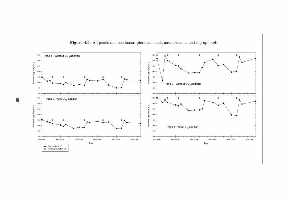
Figure 4.9: All ponds semicontinuous phase ammonia measurements and top-up levels.

69

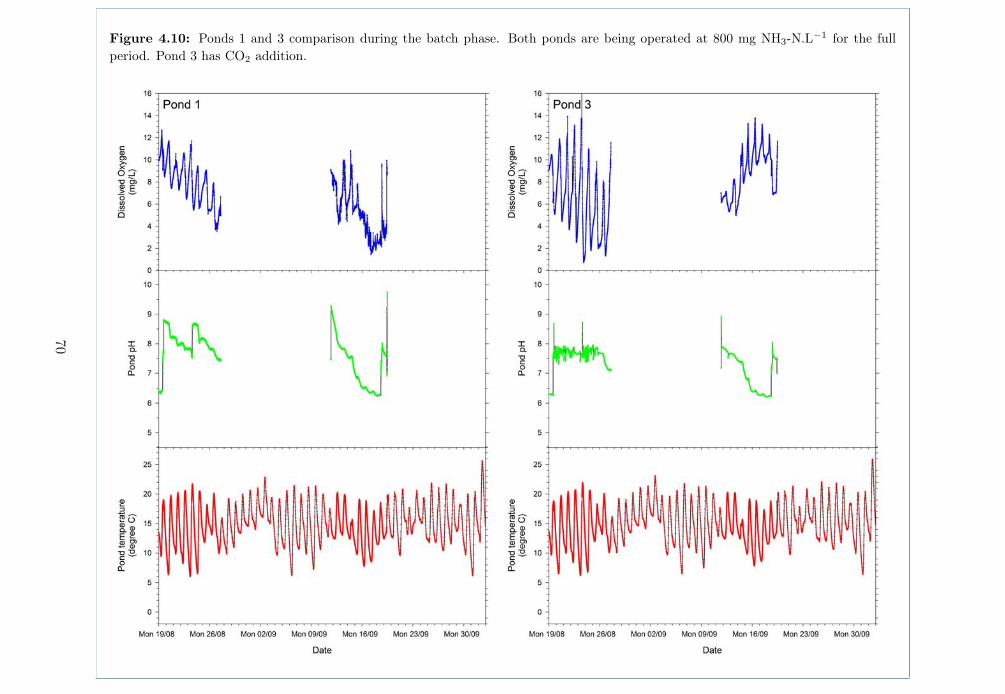
Figure 4.10: Ponds 1 and 3 comparison during the batch phase. Both ponds are being operated at 800 mg NH3-N.L�1 for the fullperiod. Pond 3 has CO2 addition.

70

Figure 4.11: Ponds 2 and 4 comparison during the batch phase. Both ponds are being operated at 1600 mg NH3-N.L�1 for the fullperiod. Pond 4 has CO2 addition.

71

Figure 4.12: All ponds semicontinuous phase cell counts.

72

Figure 4.13: Ash free dry weight analysis from all ponds during semicontinuous phase.

73

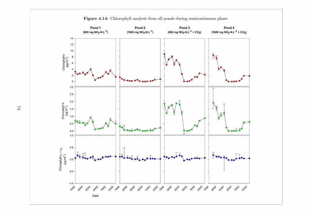
Figure 4.14: Chlorophyll analysis from all ponds during semicontinuous phase.

74

4.3 Discussion

During the bioprospecting phase of the raceway pond experiment a mixed algaeculture was established that was proven to be ultimately capable of withstandingand growing in ammonia concentrations of up to 1,600 mg NH3-N.L�1. Duringthe batch phase regular additions of ammonium chloride and KOH sustainedponds 1 and 3 at 800 mg NH3-N.L�1 while ponds 2 and 4 were increased in stepsto 1,000, 1,200 and 1,600 mg NH3-N.L�1.

Addition of CO2 to ponds 3 and 4 appears to have had the most significant effecton the chlorophyll data with the highest chlorophyll content measured in ponds3 and 4 in both batch and semicontinuous phases.

The early experiment intended to measure the difference between ammonia lossbetween an inoculated pond vs a control pond showed little or no differencebetween the two ponds. Ammonia loss to the atmosphere has been reportedelsewhere in the literature (Aguirre et al., 2011) but the expectation that ammo-nia uptake by the algae would give a higher ammonia loss above the backgroundcontrol level was not indicated in this case. This may be due to the small sizeof the inoculum in combination with the mixing effect of the paddlewheel pondsetup moving ammonia to the atmosphere quite quickly. The assumption thata 6L inoculum would be sufficient to compare with the control pond seems tohave been incorrect. A much larger inoculum may be required to measure thiseffect. It may also be possible that algae contamination in the drums or sandfilter could have had a significant inoculum effect on the control.

Through both the batch and semicontinuous phases of the experiment the chloro-phyl extraction data indicates a dominance of chlorophyll a and b with very littlec1/c2. This appears consistent with the dominance of a green algae species Leli-aert et al. (2012); Platt (1981). Observing Chlorella in all ponds throughout thecultivation also confirm this hypothesis.

It is interesting that as ammonia levels were increased step by step during thebatch phase the Chlorella cell type maintained dominance when observed duringcell counting. Other species such as Scenedesmus were found to be not dominantat any stages of the growth in ponds. A part from Scenedesmus a pennate diatomand some amoeba presence, no other eukaryotic organism was found to grow onthe wastewater for the period of the experiment. This could have been due tothe toxicity effect of high ammonium content of the anaerobic digestate effluent(Abeliovich and Azov, 1976; Källqvist and Svenson, 2003).

Interestingly in spite of the pH adjustments up to 9 all ponds responded with

75

an eventual decrease in pH back to a relatively consistent base level. Duringthe batch phase the ponds tended to return to a pH close to 7. During thesemicontinuous phase several of the ponds dropped to a pH of 6 for some time.

While the ammonium level was increased by addition of ammonium chloride,slow growth during the latter period of the semicontinuous phase could havebeen due to the low level of other nutrients. Addition of extra phosphate resultedin significant improvement in the growth of algae partially restoring the growthand health of the culture. Previous studies on algae growth have also indicatedthe importance of N:P ratio (Aguirre et al., 2011).

76

Chapter 5

General conclusions

In this study a bioprospecting strategy has been employed to allow the selectionof algal strains with potential for growth on piggery anaerobic digestion effluent.The desirable algae characteristics included tolerance to extremes of ammonium,pH and temperature, high growth rate and competitive advantage and goodperformance of photosynthesis including at high oxygen and temperature levels.

From six original promising sources dozens of algae samples were cultivated ontosynthetic and piggery sourced media at varying ammonia and pH levels. Of thesea Chlorella strain was successfully isolated from a single colony and scaled up toliquid Chu based synthetic media with an ammonia level of 500 mg NH3-N.L�1.

Under mixed culture conditions two other strains in addition to the chlorellawere observed surviving at lower cell densities but with consistent growth andperformance indicating potential for further development under the right con-ditions. These two strains were a Scenedesmus species and a pennate diatom.Other algae strains were also observed in the mixed culture such as Spirulinaand other cyanobacteria with intermittent frequency. The observation of thesestrains may be indicative of further potential for a broader range of species thatmay be isolated successfully in future if an extended bioprospecting strategywere employed over a longer time-frame, perhaps utilising a more diverse rangeof algae sources.

By utilising a combination of all bioprospecting culture sources a single racewaypond culture was established and scaled up to a total of four 1m2 outdoor paddlewheel driven raceway ponds which were used for further experiments. Runningthese four ponds in parallel a variety of batch and semicontinuous culture con-ditions were tested. The mixed strain algal culture was shown to be capable of

77

withstanding and growing in ammonia levels up to 1,600 mg NH3-N.L�1 and pHlevels up to 9 using piggery sourced anaerobic digestion effluent.

The algae was shown to be capable of surviving temperature extremes above 40°C during the bioprospecting phase of the experiment and below 5 °C during thewinter period.

Under batch phase conditions culture performance was easily maintained overa period of 5 weeks and cell counts measured were indicative of a stable algaeculture. For a period of 3 weeks a semicontinuous culture was maintained suc-cessfully. Beyond this period variations in the quality of the anaerobic digestateused appear to have influenced culture stability leading to a collapse in cultureand drop in cell growth. The reasons for the change on the effluent quality ap-pear to have been a reduction in nutrient levels in the piggery anaerobic digestioneffluent supply due to piggery maintenance and cleaning washing out much ofthe usual effluent nutrient load.

Anaerobic digestion effluent sourced early in the experiment which had beenresident in the pond for approximately one month due to piggery maintenanceperformed well during batch and semicontinuous phases of the experiment inconjunction with the algae culture acclimatised early in the bioprospecting andbatch phases of the experiment. Within the pond depths of 6 - 12cm no pre-treatment for colour was required apart from sand filtration to remove suspendedparticles.

Culture collapse on the lower quality anaerobic digestion effluent was restored byreturning the pond to batch phase conditions and via addition of phosphorousto the pond water. This result indicates that the cause of collapse was likely dueto nutrient deficiency.

5.1 Future directions

The successful growth of algae on piggery anaerobic digestion effluent as demon-strated in these experiments is a positive indicator for future application of thistechnology for piggery operations in the future. The growth of algae on anaero-bic digestion effluent with ammonium content at these high levels has never beenreported previously.

The promising results obtained in this study lead onto many questions to beasked in the course of evaluating the use of algae culture for implementationin piggery operations. Potential exists to use algae cultivated at the piggeryas either a food source to enhance pig production or as a biomass to enrich

78

the anaerobic digestion process. In order to sustain a quality controlled foodsource, growth of a single strain of algae might be the most attractive option forobtaining consistent protein, lipid and nutrient characteristics. If algae grownis merely a biomass addition to anaerobic digestion the nutritional qualities ofthe algae for livestock can be ignored however characteristics influencing biogasproduction and how this in turn cycles back to effect algae culture becomes arelevant concern. If neither of these end points are realised there is also potentialfor algae to be used and/or sold as a crop fertiliser. In this case algae productionreduces turn-around time required for anaerobic digestion effluent to be treatedin open ponds while enriching the wastewater via capture of atmospheric carbonand reducing the overall carbon footprint of the piggery. This may also allow formore effective recycling of clean water output during the algae harvest cycle.

In any of these scenarios potential exists for the piggery to convert it’s wastewaterinto a resource with benefits for the piggery and better environmental outcomes.Analysis of the options for future directions and economic evaluation on howthis might be implemented will no doubt be the subject of further study if thesepathways are to be followed. When considering these options from the currentperspective some key questions specific to the current study stand out.

In full scale algae production a semicontinuous phase would be maintained underoptimum conditions aiming at maximising the conversion of wastewater nutrientsinto algae biomass. Under such conditions typical autotroph macro-nutrientssuch as potassium or phosphorous may be limited to an extent which preventsfull utilisation of the high nitrogen levels in the culture media. Due to theaddition of potassium hydroxide to the raceway ponds during the batch andsemicontinuous phases of the experiments performed in this study any naturallyoccurring potassium limitation would not have been observed. Observations ofthe culture crashing under low phosphorous and restoration of the culture underaddition of phosphorous appear to indicate phosphorous may be a limitation ina real world piggery culture system. If phosphorous addition is required thiswould need to be sourced on the farm or imported from elsewhere. If the culturecould be provided with all nutrients for optimum growth what would the nextrate-limiting factor be?

Although an open pond culture system may seem intuitively the most econom-ically viable other pond designs might provide benefits improving light pene-tration to the pond water (incorporating the use of thin layer, optic fibres orartificial lighting), alternative pond mixing speeds or infusions of CO2 or fluegas into the pond water. The automation of culture conditions such as harvestduration, measurement of cell growth, ammonia and pH might also be desirableto simplify management of the algae culture. Incorporation of aerobic digestion

79

or other pre or post treatments may also be considered.

What would a full scale piggery system with flue gas harvested from combustedbiofuel, algae harvesting and water recycling look like? Could such a system allowclean water reuse in the piggery? How does the variability of piggery effluentduring piggery maintenance and unforeseen circumstances effect the viability ofmicroalgae culture in the piggery? Would a series of anaerobic digestion pondsbe required in order to homogenise the quality of the effluent produced by thepiggery?

This study has demonstrated the isolation and cultivation of microalgae usingundiluted piggery anaerobic digestion effluent and given an indication of the po-tential for this technology to add value and environmental benefits to the typicalpiggery in the Australian or international context. Optimisation and furtherdevelopment of microalgae culture aligns closely with the goal of providing anenvironmentally and economically optimised pig production system.

80

Bibliography

Abeliovich, A. and Azov, Y. (1976). Toxicity of ammonia to algae in sewageoxidation ponds. Applied and environmental microbiology, 31(6):801–806.

Aguirre, P., Álvarez, E., Ferrer, I., and García, J. (2011). Treatment of piggerywastewater in experimental high rate algal ponds. Revista Latinoamercicanade Biotecnología Ambiental y Algal, 2:57–66.

Ahlberg, N. R. and Boyko, B. I. (1972). Evaluation and design of aerobic di-gesters. Journal (Water Pollution Control Federation), 44(4):634–643.

APHA (2012). Standard methods for the examination of water and wastewater.American Public Health Association, 22 edition.

APL (2010a). Australian pork limited – industry survey.

APL (2010b). National environmental guidelines for piggeries / prepared by FSAConsulting for Australian Pork Limited. Australian Pork, Deakin, A.C.T.

APL (2010c). National environmental sustainability strategy for the pork indus-try 2010–2015. Technical report.

APL (2011). Sustainable piggery effluent utilisation in australian farming sys-tems. Technical report.

Azov, Y. and Goldman, J. C. (1982). Free ammonia inhibition of algal pho-tosynthesis in intensive cultures. Applied and environmental microbiology,43(4):735–739.

Barlow, E. W. R., Boersma, L., Phinney, H. K., and Miner, J. R. (1975). Algalgrowth in diluted pig waste. Agriculture and Environment, 2(4):339–355.

Bates, R. G. and Pinching, G. D. (1950). Dissociation constant of aqueousammonia at 0 to 50° from e. mf studies of the ammonium salt of a weak acid.Journal of the American Chemical Society, 72(3):1393–1396.

81

Baumgarten, E., Nagel, M., and Tischner, R. (1999). Reduction of the nitrogenand carbon content in swine waste with algae and bacteria. Applied Microbi-ology and Biotechnology, 52(2):281–284.

Beer, L. L., Boyd, E. S., Peters, J. W., and Posewitz, M. C. (2009). Engineeringalgae for biohydrogen and biofuel production. Current Opinion in Biotechnol-ogy, 20(3):264–271.

Borowitzka, M. A. (1999). Commercial production of microalgae: ponds, tanks,tubes and fermenters. Journal of Biotechnology, 70(1):313–321.

Boursier, H., Béline, F., and Paul, E. (2005). Piggery wastewater characteri-sation for biological nitrogen removal process design. Bioresource technology,96(3):351–358.

Brewer, P. G. and Goldman, J. C. (1976). Alkalinity changes generated byphytoplankton growth. Limnology and Oceanography, 21(1):108–117.

Buchanan, A., Bolton, N., Moheimani, N., Borowitzka, M., and Fallowfield, H.(2013). Algae for energy and feed: A wastewater solution. a review. Tech-nical report, Report prepared for the Co-operative Research Centre for HighIntegrity Australian Pork.

Carpenter, S. R., Caraco, N. F., Correll, D. L., Howarth, R. W., Sharpley, A. N.,and Smith, V. H. (1998). Nonpoint pollution of surface waters with phosphorusand nitrogen. Ecological Applications, 8(3):559–568.

Chadwick, D. R., Martinez, J., Marol, C., and Béline, F. (2001). Nitrogen trans-formations and ammonia loss following injection and surface application of pigslurry: a laboratory experiment using slurry labelled with 15n-ammonium. TheJournal of Agricultural Science, 136(2):231–240.

Chisti, Y. (2007). Biodiesel from microalgae. Biotechnology Advances,25(3):294–306.

Chiu, R. J., Liu, H., Chen, C. C., Chi, Y. C., Shao, H., Soong, P., and Hao, P.L. C. (1980). The cultivation of spirulina platensis on fermented swine manure.Animal Waste Treatment And Utilization.

Chu, S. (1942). The influence of the mineral composition of the medium on thegrowth of planktonic algae: part i. methods and culture media. The Journalof Ecology, pages 284–325.

Chung, P., Pond, W., Kingsbury, J., Walker, E., and Krook, L. (1978). Produc-tion and nutritive value of arthrospira platensis, a spiral blue-green alga grownon swine wastes. Journal of Animal Science, 47(2):319–330.

82

Collin, C. (2009). Biosand Filtration Of High Turbidity Water: Modified FilterDesign And Safe Filtrate Storage. PhD thesis.

Cordero, A., García, M., Herradora, M., Ramírez, G., and Martínez, R. (2010).Bacteriological characterization of wastewater samples obtained from a pri-mary treatment system on a small scale swine farm. Bioresource technology,101(9):2938–2944.

Costas, E., Flores-Moya, A., Perdigones, N., Maneiro, E., Blanco, J. L., Gar-cía, M. E., and López-Rodas, V. (2007). How eukaryotic algae can adaptto the spain’s rio tinto: a neo-darwinian proposal for rapid adaptation to anextremely hostile ecosystem. New Phytologist, 175(2):334–339.

de Godos, I., Vargas, V. A., Blanco, S., González, M. C. G., Soto, R., García-Encina, P. A., Becares, E., and Muñoz, R. (2010). A comparative evaluationof microalgae for the degradation of piggery wastewater under photosyntheticoxygenation. Bioresource technology, 101(14):5150–5158.

de Victorica-Almeida, J., Galván-García, M., and Ayala-Ruiz, R. (2008). Sustain-able management of effluents from small piggery farms in mexico. AmericanJournal of Environmental Sciences, 4(3):185–188.

Dimpl, E. (2010). Small-scale electricity generation from biomass. part ii: Biogas.Technical report.

Dor, I. (1975). High density, dialysis culture of algae on sewage. Water Research,9(3):251–254.

Douskova, I., Doucha, J., Livansky, K., Machat, J., Novak, P., Umysova, D.,Zachleder, V., and Vitova, M. (2009). Simultaneous flue gas bioremediationand reduction of microalgal biomass production costs. Applied Microbiologyand Biotechnology, 82(1):179–185.

Evans, M. R., Smith, M. P. W., Deans, E. A., Svoboda, I. F., and Thacker,F. E. (1986). Nitrogen and aerobic treatment of slurry. Agricultural Wastes,15(3):205–213.

Fallowfield, H. J. and Garrett, M. K. (1985). The photosynthetic treatment ofpig slurry in temperate climatic conditions: A pilot-plant study. AgriculturalWastes, 12(2):111–136.

Fenlon, D. R. and Mills, P. J. (1980). On farm aerobic treatment of piggery waste.the effect of residence time and storage on effluent quality. Water Research,14(7):805–805.

83

Finlayson, M., Chick, A., von Oertzen, I., and Mitchell, D. (1987). Treatment ofpiggery effluent by an aquatic plant fiber. Biological Wastes, 19(3):179–196.

Gupta, S. and Agrawal, S. C. (2007). Survival and reproduction in some algaeunder stress conditions. Folia Microbiologica, 52(6):603–617.

Hamasaki, A., Shioji, N., Ikuta, Y., Hukuda, Y., Makita, T., Hlrayama, K.,Matuzaki, H., Tukamoto, T., and Sasaki, S. (1994). Carbon dioxide fixationby microalgal photosynthesis using actual flue gas from a power plant. AppliedBiochemistry and Biotechnology, 45-46(1):799–809.

Hashimoto, S. and Furukawa, K. (1989). Nutrient removal from secondary ef-fluent by filamentous algae. Journal of Fermentation and Bioengineering,67(1):62–69.

Hoshaw, R. W. (1961). Sexual cycles of three green algae for laboratory study.The American Biology Teacher, 23(8):489–499.

Hu, B. (2013). Development of an effective swine manure-based algal cultivationsystem for biofuel and animal feed production and wastewater treatment. Ph.d.

Jeffrey, S. W. T. and Humphrey, G. F. (1975). New spectrophotometric equationsfor determining chlorophylls a, b, c1 and c2 in higher plants, algae and naturalphytoplankton. Biochem. Physiol. Pflanz, 167(19):1–194.

Ji, M.-K., Jeon, B.-H., Kim, H.-C., Sapireddy, V. R., Yun, H.-S., Abou-Shanab,R. A. I., Choi, J., Lee, W., Timmes, T. C., and Inamuddin (2013). Simultane-ous nutrient removal and lipid production from pretreated piggery wastew-ater by chlorella vulgaris ysw-04. Applied microbiology and biotechnology,97(6):2701–2710.

Kebede-Westhead, E., Pizarro, C., and Mulbry, W. (2006). Treatment of swinemanure effluent using freshwater algae: Production, nutrient recovery, andelemental composition of algal biomass at four effluent loading rates. Journalof Applied Phycology, 18(1):41–46.

Krapac, I. G., Dey, W. S., Roy, W. R., Smyth, C. A., Storment, E., Sargent,S. L., and Steele, J. D. (2002). Impacts of swine manure pits on groundwaterquality. Environmental Pollution, 120(2):475–492.

Källqvist, T. and Svenson, A. (2003). Assessment of ammonia toxicity in testswith the microalga, nephroselmis pyriformis, chlorophyta. Water Research,37(3):477–484.

84

Leitão, R. C., van Haandel, A. C., Zeeman, G., and Lettinga, G. (2006). Theeffects of operational and environmental variations on anaerobic wastewatertreatment systems: A review. Bioresource Technology, 97(9):1105–1118.

Leliaert, F., Smith, D. R., Moreau, H., Herron, M. D., Verbruggen, H., Delwiche,C. F., and De Clerck, O. (2012). Phylogeny and molecular evolution of thegreen algae. Critical Reviews in Plant Sciences, 31(1):1–46.

Lettinga, G., Hulshoff-Pol, L., and Zeeman, G. (1999). Lecture notes: Biologicalwastewater treatment; part i anaerobic wastewater treatment.

Lim, B. and Headberry-Partners-P/L (2004). Australian pork limited project1915: Renewal energy industry development report on technical, economic andfinancial implications of using piggery waste to generate electricity. Technicalreport.

Liu, J., Ge, Y., Cheng, H., Wu, L., and Tian, G. (2013). Aerated swine la-goon wastewater: a promising alternative medium for botryococcus brauniicultivation in open system. Bioresource Technology.

Lopez-Rodas, V., Agrelo, M., Carrillo, E., Ferrero, L., Larrauri, A., Martín-Otero, L., and Costas, E. (2001). Resistance of microalgae to modern watercontaminants as the result of rare spontaneous mutations. European Journalof Phycology, 36(2):179–190.

Maeda, M. and Kato, K. (1995). Dissociation constants of ammonium ion andactivity coefficients of ammonia in ammonium nitrate solutions. Journal ofChemical and Engineering Data, 40(1):253–256.

Maraseni, T. N. and Maroulis, J. (2008). Piggery: From environmental pollutionto a climate change solution. Journal of Environmental Science and HealthPart B, 43(4):358–363.

McGriff Jr, E. C. and McKinney, R. E. (1972). The removal of nutrients andorganics by activated algae. Water Research, 6(10):1155–1164.

Moheimani, N. R. (2005). The culture of coccolithophorid algae for carbon dioxidebioremediation. PhD thesis.

Moheimani, N. R. (2012). Inorganic carbon and ph effect on growth and lipidproductivity of tetraselmis suecica and chlorella sp (chlorophyta) grown out-doors in bag photobioreactors. Journal of Applied Phycology, 25(2):387–398.

Moheimani, N. R. and Borowitzka, M. A. (2006). The long-term culture ofthe coccolithophore pleurochrysis carterae (haptophyta) in outdoor racewayponds. Journal of Applied Phycology, 18(6):703–712.

85

Moheimani, N. R. and Borowitzka, M. A. (2011). Increased co2 and the ef-fect of ph on growth and calcification of pleurochrysis carterae and emilianiahuxleyi (haptophyta) in semicontinuous cultures. Applied Microbiology andBiotechnology, 90(4):1399–407.

Mutanda, T., Ramesh, D., Karthikeyan, S., Kumari, S., Anandraj, A., andBux, F. (2011). Bioprospecting for hyper-lipid producing microalgal strainsfor sustainable biofuel production. Bioresource Technology, 102(1):57–70.

Olguin, E. J., Galicia, S., Mercado, G., and Perez, T. (2003). Annual productivityof spirulina (arthrospira) and nutrient removal in a pig wastewater recyclingprocess under tropical conditions. Journal of Applied Phycology, 15(2-3):249–257.

O’Neill, D. H. and Phillips, V. R. (1991). A review of the control of odournuisancefrom livestock buildings: Part 1, influence of the techniques for man-aging waste within the building. Journal of Agricultural Engineering Research,50(0):1–10.

Ong, H., Lim, Y., and Suhaimi, M. (2006). Environmental impact and removal ofphosphates in swine farm effluent. Journal Of Tropical Agriculture And FoodScience, 34(2):355.

Oswald, W. J. and Gotaas, H. B. (1955). Photosynthesis in sewage treatment.Trans. Am. Soc. Civ. Eng, 122:73–105.

Padgett, W. J. (1975). A stochastic model for stream pollution. MathematicalBiosciences, 25(3):309–317.

Padgett, W. J. (1978). A stream-pollution model with random deoxygenationand reaeration coefficients. Mathematical Biosciences, 42(1):137–148.

Park, J., Jin, H.-F., Lim, B.-R., Park, K.-Y., and Lee, K. (2010a). Ammoniaremoval from anaerobic digestion effluent of livestock waste using green algascenedesmus sp. Bioresource Technology, 101(22):8649–8657.

Park, J. B. K., Craggs, R. J., and Shilton, A. N. (2010b). Wastewater treat-ment high rate algal ponds for biofuel production. Bioresource Technology,102(1):35–42.

Payne, R. W. (1984). Chemical, physical and microbial characteristics of pigexcreta. Technical report, Western Australian Department of Agriculture.

Pink, B. (2012). 2012 Year book Australia. Canberra : Australian Bureau ofStatistics.

86

Pisarevsky, A., Polozova, I., and Hockridge, P. (2005). Chemical oxygen demand.Russian Journal of Applied Chemistry, 78(1):101–101.

Platt, T. (1981). Physiological bases of phytoplankton ecology. Bulletin / Cana-dian Bulletin of Fisheries and Aquatic Sciences;no. 210. Department of Fish-eries and Oceans, Ottawa.

Ramírez, G., Martínez, R., Herradora, M., Castrejón, F., and Galvan, E. (2005).Isolation of salmonella spp. from liquid and solid excreta prior to and followingensilage in ten swine farms located in central mexico. Bioresource Technology,96(5):587–595.

Ratha, S. K., Prasanna, R., Gupta, V., Dhar, D. W., and Saxena, A. K.(2012). Bioprospecting and indexing the microalgal diversity of different eco-logical habitats of india. World Journal of Microbiology and Biotechnology,28(4):1657–1667.

Rudd, J. W. M., Kelly, C. A., Schindler, D. W., and Turner, M. A. (1988).Disruption of the nitrogen cycle in acidified lakes. Science, 240(4858):1515.

Sharma, B. and Ahlert, R. C. (1977). Nitrification and nitrogen removal. WaterResearch, 11(10):897–897.

Sowers, K. R. (2009). Methanogenesis, pages 265–286. Academic Press, Oxford.

Strain, J. J., Fallowfield, H. J., Fraser, T. W., and Garrett, M. K. (1986). A nu-tritional evaluation of farm waste grown and axenically cultured algal biomass.Agricultural Wastes, 15(4):235–252.

Sullivan, A. B., Snyder, D. M., and Rounds, S. A. (2010). Controls on biochem-ical oxygen demand in the upper klamath river, oregon. Chemical Geology,269(1):12–21.

Svoboda, I. (1995). Nitrogen removal from pig slurry by nitrification and denitri-fication. Proceedings of the 7th International Symposium on Agricultural andFood Processing Wastes (ISAFPW95). ASAE, St. Joseph, MI, pages 24–33.

Sánchez-Fortún, S., López-Rodas, V., Navarro, M., Marvá, F., D’Ors, A., Rouco,M., Haigh-Florez, D., and Costas, E. (2009). Toxicity and adaptation of dic-tyosphaerium chlorelloides to extreme chromium contamination. Environmen-tal toxicology and chemistry / SETAC, 28(9):1901–1905.

Teschler, L. (2009). Algae automation. Machine Design, 81(5):73–75.

Ugwu, C. U., Aoyagi, H., and Uchiyama, H. (2008). Photobioreactors for masscultivation of algae. Bioresource Technology, 99(10):4021–4028.

87

Ushikubo, A., Yoshimura, M., Kato, M., Oyama, G., and D’Itri, F. M. (1991).Livestock waste treatment in a double channel oxidation ditch. Agriculture,Ecosystems and Environment, 36(1–2):59–74.

Vanotti, M. B., Szogi, A. A., and Vives, C. A. (2008). Greenhouse gas emissionreduction and environmental quality improvement from implementation of aer-obic waste treatment systems in swine farms. Waste Management, 28(4):759–766.

Woltemade, C. J. (2000). Ability of restored wetlands to reduce nitrogen andphosphorous concentrations in agricultural drainage water. Journal of Soil andWater Conservation, 55(3):303.

Yun, Y., Lee, S. B., Park, J. M., Lee, C., and Yang, J. (1997). Carbon dioxidefixation by algal cultivation using wastewater nutrients. Journal of ChemicalTechnology and Biotechnology, 69(4):451–455.

Zhou, W., Li, Y., Min, M., Hu, B., Chen, P., and Ruan, R. (2011). Local bio-prospecting for high-lipid producing microalgal strains to be grown on concen-trated municipal wastewater for biofuel production. Bioresource Technology,102(13):6909–6919.

88