micro data and macro technology - devesh r. raval · micro data and macro technology ezra ober eld...
TRANSCRIPT
Micro Data and Macro Technology∗
Ezra Oberfield
Princeton University & NBER
Devesh Raval
Federal Trade Commission
August 29, 2014
Abstract
We develop a framework to estimate the aggregate capital-labor elasticity of substitution by
aggregating the actions of individual plants, and use it to assess the decline in labor’s share of
income in the US manufacturing sector. The aggregate elasticity reflects substitution within
plants and reallocation across plants; the extent of heterogeneity in capital intensities deter-
mines their relative importance. We use micro data on the cross-section of plants to build up
to the aggregate elasticity at a point in time. Our approach places no assumptions on the evo-
lution of technology, so we can separately identify shifts in technology and changes in response
to factor prices. We find that the aggregate elasticity for the US manufacturing sector has
been stable since 1970 at about 0.7. Mechanisms that work solely through factor prices cannot
account for the labor share’s decline. Finally, the aggregate elasticity is substantially higher in
less-developed countries.
KEYWORDS: Elasticity of Substitution, Aggregation, Labor Share, Bias of Technical Change.
∗First version: January 2012. We thank Enghin Atalay, Bob Barsky, Ehsan Ebrahimy, Ali Hortacsu,Konstantin Golyaev, Michal Kolesar, Sam Kortum, Lee Lockwood, Harry J. Paarsch, Richard Rogerson,Chad Syverson, Hiroatsu Tanaka, and Nate Wilson for their comments on this paper, and Loukas Karabar-bounis for his comments as a discussant. We are grateful to Frank Limehouse for all of his help at theChicago Census Research Data Center and to Jon Samuels and Dale Jorgenson for providing us with capitaltax information and estimates. Any opinions and conclusions expressed herein are those of the authors anddo not necessarily represent the views of the U.S. Census Bureau or the Federal Trade Commission and itsCommissioners. All results have been reviewed to ensure that no confidential information is disclosed.
1 Introduction
Over the last several decades, labor’s share of income in the US manufacturing sector has
fallen by more than 15 percentage points.1 A variety of mechanisms have been proposed to
explain declining labor shares; these can be separated into two categories. Some reduce the
labor share solely by altering factor prices. For example, Piketty (2014) maintained that
declining labor shares resulted from increased capital accumulation, and Karabarbounis and
Neiman (2014) argued that they stem from falling capital prices. Other mechanisms, such
as automation and offshoring, would be viewed through the lens of an aggregate production
function as a change in technology.2
As Hicks (1932) first pointed out, the crucial factor in assessing the relevance of these
mechanisms is the aggregate capital-labor elasticity of substitution, which governs how ag-
gregate factor shares respond to changing factor prices. More generally, as a central feature
of aggregate technology, the elasticity helps answer a wide variety of economic questions.
These include, for example, the welfare impact of corporate tax changes, the impact of in-
ternational interest rate differentials on output per worker, the speed of convergence to a
steady state, and how trade barriers shape patterns of specialization.3
Unfortunately, obtaining the elasticity is difficult; Diamond et al. (1978) proved that
the elasticity cannot be identified from time series data on output, inputs, and marginal
products alone. Instead, identification requires factor price movements that are independent
of the bias of technical change. Economists have thus explored two different approaches to
estimating the elasticity.
1The overall labor share has declined by roughly 8 percentage points over the same time period. While themanufacturing sector is relatively small, representing 13 percent of value added and 8 percent of employmentin 2010 (24 percent and 27 percent respectively in 1970), it accounts for between 30 percent and 45 percentof decline in the overall labor share, depending on whether the counterfactual freezes the manufacturinglabor share at its 1970 level or both manufacturing’s labor share and its share of value added at its 1970level.
2Formally, changes in factor compensation can be decomposed into the response to shifts in factor prices(holding technology fixed) and changes due to shifts in technology (holding factor prices fixed). We callthe latter the “bias of technical change,” and we use the term loosely to include everything other thanfactor prices, including changes in production possibilities or in composition due to changing tastes or trade.Changes in the supply of capital or labor (as in Piketty (2014)) would alter relative factor prices but leavetechnology unchanged.
3See Hall and Jorgenson (1967), Mankiw (1995), and Dornbusch et al. (1980).
1
The first approach uses the aggregate time series and places strong parametric assump-
tions on the aggregate production function and bias of technical change for identification.
The most common assumptions are that there has been no bias or a constant bias over time.
Leon-Ledesma et al. (2010) demonstrated that, even under these assumptions, it is difficult
to obtain the true aggregate elasticity. Not surprisingly, the estimates found in this literature
range widely from 0.5 to 1.5, hindering inference about the decline in the labor share.4
The second approach uses micro production data with more plausibly exogenous variation
in factor prices, and yields the micro capital-labor elasticity of substitution. Houthakker
(1955), however, famously showed that the micro and macro elasticities can be very different;
an economy of Leontief micro units can have a Cobb–Douglas aggregate production function.5
Given Houthakker’s result, it is unclear whether the micro elasticity can help answer the
many questions that hinge on the aggregate elasticity.
In this paper, we show how the aggregate elasticity of substitution can be recovered from
the plant-level elasticity. Building on Sato (1975), we show that the aggregate elasticity is a
convex combination of the plant-level elasticity of substitution and the elasticity of demand.6
In response to a wage increase, plants substitute towards capital. In addition, capital-
intensive plants gain market share from labor-intensive plants. The degree of heterogeneity
in capital intensities determines the relative importance of within-plant substitution and
reallocation. For example, when all plants produce with the same capital intensity, there is
no reallocation of resources across plants.
Using this framework, we build the aggregate capital-labor elasticity from its individ-
ual components. We estimate micro production and demand parameters. Since Levhari
(1968), it has been well known that Houthakker’s result of a unitary elasticity of substitu-
4Although Berndt (1976) found a unitary elasticity of substitution in the US time series assuming neutraltechnical change, Antras (2004) and Klump et al. (2007) subsequently found estimates from 0.5 to 0.9allowing for biased technical change. Karabarbounis and Neiman (2014) estimate an aggregate elasticity of1.25 using cross-country panel variation in capital prices. Piketty (2014) estimates an aggregate elasticitybetween 1.3 and 1.6. Herrendorf et al. (2014) estimate an elasticity of 0.84 for the US economy as a wholeand 0.80 for the manufacturing sector. Alvarez-Cuadrado et al. (2014) estimate an elasticity of 0.78 for themanufacturing sector.
5Houthakker assumed that factor-augmenting productivities follow independent Pareto distributions. Theconnection between Pareto distributions and a Cobb-Douglas aggregate production function is also empha-sized in Jones (2005), Lagos (2006), and Luttmer (2012).
6Sato (1975) showed this for a two-good economy. See also Miyagiwa and Papageorgiou (2007).
2
tion is sensitive to the distribution of capital intensities. Rather than making distributional
assumptions, we directly measure the empirical distribution using cross-sectional micro data.
Thus, given the set of plants that existed at a point in time, we estimate the aggregate
elasticity of substitution at that time. Our strategy allows both the aggregate elasticity and
the bias of technical change to vary freely over time, opening up a new set of questions.
Because our identification does not impose strong parametric assumptions on the time path
of the bias, our approach is well suited for measuring how the bias has varied over time
and how it has contributed to the decline in labor’s share of income. We can also examine
how the aggregate elasticity has changed over time and whether it varies across countries at
different stages of development.
We first estimate the aggregate elasticity for the US manufacturing sector using the
US Census of Manufactures. In 1987, our benchmark year, we find an average plant-level
elasticity of substitution of roughly one-half. Given the heterogeneity in capital shares and
our estimates of other parameters, the aggregate elasticity in 1987 was 0.71.7 Reallocation
thus accounts for roughly one-third of substitution. Despite large structural changes in
manufacturing over the past forty years,8 the aggregate elasticity has been stable. We find
the elasticity has risen slightly from 0.67 in 1972 to 0.75 in 2007.
We then use this estimate to decompose the decline in labor’s share of income in the man-
ufacturing sector since 1970. We have several findings. First, since our estimated aggregate
elasticity is below one, mechanisms such as increased capital accumulation or declining cap-
ital prices would raise the labor share. Second, the contribution of factor prices to the labor
share exhibits little variation over time, and thus does not match the accelerating decline of
the labor share. Rather, the acceleration is accounted for by changes in the pace of the bias
of technical change. Third, wages grew more slowly before 1970; a counterfactual exercise
that keeps wage growth at its pre-1970 pace indicates that this can explain about one sixth
of the decline in the labor share. Finally, a shift in the composition of industries accounts
for part of the acceleration in the labor share’s decline since 2000. These findings suggest
7Our estimate is a long-run elasticity of substitution between capital and labor, owing to a proper inter-pretation of our estimates of plant-level parameters. It is thus an upper bound on the short run elasticity.
8Elsby et al. (2013) have emphasized the shift in industry composition in the context of labor’s share ofincome.
3
the decline in the labor share stems from factors that affect technology, broadly defined, in-
cluding automation and offshoring, rather than mechanisms that work solely through factor
prices.
Finally, our approach allows us to examine how the shape of technology varies across
countries at various stages of development; policies or frictions that lead to more variation in
capital shares raise the aggregate elasticity. Using their respective manufacturing censuses,
we find an average manufacturing sector elasticity of 0.84 for Chile, 0.84 for Colombia, and
1.11 for India. These differences are quantitatively important; the response of output per
worker to a change in the interest rate is over fifty percent larger in India than in the US,
as is the welfare cost of capital taxation. They also imply that a decline in capital prices
decreases the labor share in India but increases it in the US.
Our work complements the broad literature that examines how changes in factor prices
and technology have affected the distribution of income. Krusell et al. (2000) studied how a
capital-skill complementarity and a declining price of capital can change factor shares and
raise the skill premium. Acemoglu (2002), Acemoglu (2003), and Acemoglu (2010) showed
how factor prices and the aggregate capital-labor elasticity of substitution can determine the
direction of technical change. Burstein et al. (2014) studied how changes in technology and
supplies of various factors alter factor compensation. Autor et al. (2003) and Autor et al.
(2013) studied how changes in technology and trade affect factor income.
The remainder of the paper is organized as follows. In Section 2, we present our theoretical
analysis of the aggregation problem, while in Section 3 we estimate the aggregate elasticity
for manufacturing. Section 4 examines the robustness of our estimates. In Section 5, we
use our estimates of the aggregate elasticity to assess the changes in the labor share. In
Section 6, we examine how the aggregate elasticity varies across countries and discuss policy
implications. Finally, in Section 7 we conclude.
2 Theory
This section characterizes the aggregate elasticity of substitution between capital and labor in
terms of production and demand elasticities of individual plants. We begin with a simplified
4
environment in which we describe the basic mechanism and intuition. We proceed to enrich
the model with sufficient detail to take the model to the data by incorporating materials and
allowing for heterogeneity across industries.
A number of features—adjustment costs, an extensive margin, non-constant returns to
scale, imperfect pass-through, and varying production and demand elasticities across plants
in the same industry—are omitted from our benchmark model. We postpone a discussion of
these until Section 4.
2.1 Simple Example
Consider a large set of plants I whose production functions share a common, constant elas-
ticity of substitution between capital and labor, σ. A plant produces output Yi from capital
Ki and labor Li using the following CES production function:
Yi =[(AiKi)
σ−1σ + (BiLi)
σ−1σ
] σσ−1
(1)
Productivity differences among plants are factor augmenting: Ai is i’s capital-augmenting
productivity and Bi i’s labor-augmenting productivity.
Consumers have Dixit–Stiglitz preference across goods, consuming the bundle Y =(∑i∈I D
1εi Y
ε−1ε
i
) εε−1
. Plants are monopolistically competitive, so each plant faces an isoelas-
tic demand curve with a common elasticity of demand ε > 1.
Among these plants, aggregate demand for capital and labor are defined as K ≡∑
i∈I Ki
and L ≡∑
i∈I Li respectively. We define the aggregate elasticity of substitution, σagg, to be
the partial equilibrium response of the aggregate capital-labor ratio, K/L, to a change in
relative factor prices, w/r:9
σagg ≡ d lnK/L
d lnw/r(2)
We neither impose nor derive a parametric form for an aggregate production function. Given
the allocation of capital and labor, σagg simply summarizes, to a first order, how a change
in factor prices would affect the aggregate capital-labor ratio.
9Since production and demand are homogeneous of degree one, a change in total spending would notalter the aggregate capital-labor ratio. We address non-homothetic environments in Web Appendix B.6.
5
Let αi ≡ rKirKi+wLi
and α ≡ rKrK+wL
denote the cost shares of capital for plant i and in
aggregate. The plant-level and industry-level elasticities of substitution are closely related
to the changes in these capital shares:
σ − 1 =d ln rKi/wLi
d lnw/r=
d lnαi/(1− αi)d lnw/r
=1
αi(1− αi)dαi
d lnw/r(3)
σagg − 1 =d ln rK/wL
d lnw/r=
d lnα/(1− α)
d lnw/r=
1
α(1− α)
dα
d lnw/r(4)
The aggregate cost share of capital can be expressed as an average of plant capital shares,
weighted by size:
α =∑i∈I
αiθi (5)
where θi ≡ rKi+wLirK+wL
denotes plant i’s expenditure on capital and labor as a fraction of
the aggregate expenditure. To find the aggregate elasticity of substitution, we can simply
differentiate equation (5):
dα
d lnw/r=
∑i∈I
dαid lnw/r
θi +∑i∈I
αidθi
d lnw/r
Using equations 3 and 4, this can be written as
σagg − 1 =1
α(1− α)
∑i∈I
αi(1− αi)(σ − 1)θi +1
α(1− α)
∑i∈I
αiθid ln θi
d lnw/r(6)
The first term on the right hand side is a substitution effect that captures the change in
factor intensity holding fixed each plant’s size, θi. σ measures how much an individual plant
changes its mix of capital and labor in response to changes in factor prices. The second term
is a reallocation effect that captures how plants’ sizes change with relative factor prices. By
Shephard’s Lemma, a plant’s cost share of capital αi measures how relative factor prices
affect its marginal cost. When wages rise, plants that use capital more intensively gain a
relative cost advantage. Consumers respond to the subsequent changes in relative prices by
shifting consumption toward the capital intensive goods. This reallocation effect is larger
6
when demand is more elastic, because customers respond more to changing relative prices.
Formally, the change in i’s relative expenditure on capital and labor is
d ln θid lnw/r
= (ε− 1) (αi − α) (7)
After some manipulation (see Appendix A for details), we can show that the industry elas-
ticity of substitution is a convex combination of the micro elasticity of substitution and
elasticity of demand:
σagg = (1− χ)σ + χε (8)
where χ ≡∑
i∈I(αi−α)2α(1−α) θi.
The first term, (1− χ)σ, measures substitution between capital and labor within plants.
The second term, χε, captures reallocation between capital- and labor-intensive plants.
We call χ the heterogeneity index. It is proportional to the cost-weighted variance of
capital shares and lies between zero and one.10 When each plant produces at the same
capital intensity, χ is zero and there is no reallocation across plants. Each plant’s marginal
cost responds to factor price changes in the same way, so relative output prices are unchanged.
In contrast, if some plants produce using only capital while all others produce using only
labor, all factor substitution is across plants and χ is one. When there is little variation in
capital intensities, within-plant substitution is more important than reallocation.
2.2 Baseline Model
This section describes the baseline model we will use in our empirical implementation. The
baseline model extends the previous analysis by allowing for heterogeneity across industries
and using a production structure in which plants use materials in addition to capital and
labor.
Let N be the set of industries and In be the set of plants in industry n. We assume that
each plant’s production function has a nested CES structure.
10A simple proof:∑i∈I (αi − α)
2θi =
∑i∈I α
2i θi − α2 ≤
∑i∈I αiθi − α2 = α − α2 = α(1− α). It follows
that χ = 1 if and only if each plant uses only capital or only labor (i.e., for each i, αi ∈ {0, 1}).
7
Assumption 1 Plant i in industry n produces with the production function
Fni (Kni, Lni,Mni) =
([(AniKni)
σn−1σn + (BniLni)
σn−1σn
] σnσn−1
ζn−1ζn
+ (CniMni)ζn−1ζn
) ζnζn−1
(9)
so its elasticity of substitution between capital and labor is σn. Further, i’s elasticity of
substitution between materials and its capital-labor bundle is ζn.
We also assume that demand has a nested structure with a constant elasticity at each
level of aggregation. Such a structure is consistent with a representative consumer whose
preferences exhibit constant elasticities of substitution across industries and across varieties
within each industry:
Y ≡
[∑n∈N
D1ηn Y
η−1η
n
] ηη−1
, Yn ≡
(∑i∈In
D1εnni Y
εn−1εn
ni
) εnεn−1
(10)
This demand structure implies that each plant in industry n faces a demand curve with
constant elasticity εn. Letting q be the price of materials, each plant maximizes profit
maxPni,Yni,Kni,Lni,Mni
PniYni − rKni − wLni − qMni
subject to the technological constraint Yni = Fni (Kni, Lni,Mni) and the demand curve Yni =
Yn(Pni/Pn)−εn , where Pn ≡(∑
i∈In DniP1−εnni
) 11−εn is the price index for industry n.
The industry-level elasticity of substitution between capital and labor for industry n
measures the response of the industry’s capital-labor ratio to a change in relative factor
prices:
σNn ≡d lnKn/Ln
d lnw/r
The derivation of this industry elasticity of substitution follows Section 2.1 up to equa-
tion (6). As before, αni = rKnirKni+wLni
is plant i’s capital share of non-materials cost and
θni = rKni+wLnirKn+wLn
plant i’s share of industry n’s expenditure on capital and labor. We will
show that reallocation depends on plants’ expenditures on materials. We denote plant i’s
materials share of its total cost as sMni ≡qMni
rKni+wLni+qMni. Because producers of intermediate
inputs use capital and labor, changes in r and w would impact the price of materials. We
8
define αM ≡ d ln q/wd ln r/w
to be the capital content of materials.
Proposition 1 Under Assumption 1, the industry elasticity of substitution is:
σNn = (1− χn)σn + χn[(1− s̄Mn )εn + s̄Mn ζn
]where χn =
∑i∈In
(αni−αn)2αn(1−αn) θni and s̄Mn =
∑i∈In (αni−αn)(αni−α
M )θnisMni∑
i∈In (αni−αn)(αni−αM )θni
The proofs of all propositions are contained in Appendix A.
Relative to equation (8), the demand elasticity is replaced by a convex combination of the
elasticity of demand, εn, and the elasticity of substitution between materials and the capital-
labor bundle, ζn. This composite term measures the change in i’s share of its industry’s
expenditure on capital and labor, θni. Intuitively, a plant’s expenditure on capital and labor
can fall because its overall scale declines or because it substitutes towards materials. The cost
share of materials determines the relative importance of each. As materials shares approach
zero, all shifts in composition are due to changes in scale, and Proposition 1 reduces to
equation (8). In contrast, as a plant’s materials share approaches one, changes in its cost
of capital and labor have a negligible impact on its marginal cost, and hence a negligible
impact on its sales. Rather, the change in its expenditure on capital and labor is determined
by substitution between materials and the capital-labor bundle.
The aggregate elasticity parallels the industry elasticity; aggregate capital-labor substi-
tution consists of substitution within industries and reallocation across industries. Propo-
sition 2 shows that expression for the aggregate elasticity parallels the expressions for the
industry elasticity in Proposition 1 with plant and industry variables replaced by industry
and aggregate variables respectively.
Proposition 2 The aggregate elasticity between capital and labor, σagg = d lnK/Ld lnw/r
, is:
σagg = (1− χagg) σ̄N + χagg[(1− s̄M)η + s̄M ζ̄N
](11)
where χagg ≡∑
n∈N(αn−α)2α(1−α) θn, s̄M ≡
∑n∈N
(αn−α)(αn−αM )θn∑n′∈N (αn′−α)(αn′−αM )θn′
sMn ,
σ̄N ≡∑
n∈Nαn(1−αn)θn∑
n′∈N αn′ (1−αn′ )θnσNn , and ζ̄N ≡
∑n∈N
(αn−α)(αn−αM )θnsMn∑n′∈N (αn′−α)(αn′−αM )θn′s
Mn′ζNn .
9
Substitution within industries depends on σ̄N , a weighted average of the industry elasticities
of substitution defined in Proposition 1. ζ̄N is similarly a weighted average of industry level
elasticities of substitution between materials and non-materials (we relegate the expression
ζNn to Appendix A). χagg is the cross-industry heterogeneity index and is proportional to
the cost-weighted variance of industry capital shares.
3 US Aggregate Elasticity of Substitution
The methodology developed in the previous section shows how to recover the aggregate
capital-labor elasticity from micro parameters and the distribution of plant expenditures. We
now use plant-level data on US manufacturing plants to estimate all of the micro components
of the aggregate elasticity. We then assemble these components to estimate the aggregate
capital-labor elasticity of substitution for the US manufacturing sector and examine its
behavior over time.
3.1 Data
The two main sources of micro data on manufacturing plants are the US Census of Manufac-
tures and Annual Survey of Manufactures (ASM). The Census of Manufactures is a census
of all manufacturing plants conducted every five years. It contains more than 180,000 plants
per year.11 The Annual Survey of Manufactures tracks about 50,000 plants over five year
panel rotations between Census years, and includes the largest plants with certainty.
In this study, we primarily use factor shares measured at the plant level. For the Census
samples, we measure capital by the end year book value of capital, deflated using an industry
specific current cost to historic cost deflator. The ASM has the capital and investment
history required to construct perpetual inventory measures of capital. Thus, we create
perpetual inventory measures of capital, accounting for retirement data from 1973 to 1987
as in Caballero et al. (1995) and using NIPA investment deflators for each industry-capital
type. Capital costs consist of the total stock of structures and equipment capital multiplied
11This excludes small Administrative Record plants with fewer than five employees, for whom the Censusonly tracks payroll and employment. We omit these in line with the rest of the literature using manufacturingCensus data.
10

by the appropriate rental rate, using a Jorgensonian user cost of capital based upon an
external real rate of return of 3.5 percent as in Harper et al. (1989). For labor costs, both
surveys contain total salaries and wages at the plant level, but the ASM subsample includes
data on supplemental labor costs including benefits as well as payroll and other taxes. For
details about data construction, see Web Appendix C.
The Census of Manufactures, unlike the ASM subsample, only contains capital data
beginning in 1987. Further, industry definitions change from SIC to NAICS in 1997. Given all
of these considerations, we take the following approach to estimating the aggregate elasticity.
We use the full 1987 Census of Manufactures to estimate the micro elasticities and ex-
amine their robustness. We then use the ASM in each year for the relevant information
on the composition of plants – the heterogeneity indices and materials shares – because we
extend the analysis from 1972 to 2007. So, for example, to compute the aggregate elasticity
of substitution in 1977, we combine estimates of micro parameters from the 1987 Census of
Manufactures with information from the 1977 ASM.
Throughout, we use a plant’s total cost of labor as a measure of its labor input. We
view employees of different skill as supplying different quantities of efficiency units of labor,
so using the wage bill controls for differences in skill. In Section 4.4 we show that our
methodology is valid even if wages per efficiency unit of labor vary across plants.
3.2 Micro Heterogeneity
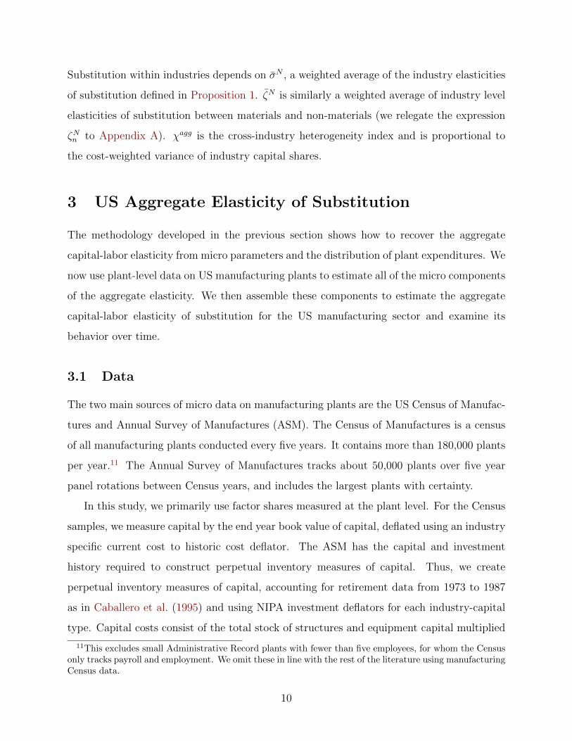
The extent of heterogeneity in capital intensities, as measured by the heterogeneity index,
determines the relative importance of within-plant substitution and reallocation. Figure 1a
depicts these indices for each industry in 1987. Across industries, the indices average 0.1 and
are all less than 0.2. Similarly, Figure 1b shows how the average heterogeneity index evolves
over time. While heterogeneity indices are rising, they remain relatively small. Industry
capital shares exhibit even less variation; the cross-industry heterogeneity index χagg is 0.05.12
Given this level of heterogeneity, the plant-level elasticity of substitution between capital
12It may seem surprising that these heterogeneity indices are so small. Note, however, that the numeratorof the heterogeneity index is a cost-weighted variance of capital shares, which would likely be smaller thanan unweighted variance. In addition, since capital shares are less than one, their variance is smaller thantheir standard deviation.
11
(a) Heterogeneity Indices Across Industries (b) Heterogeneity Indices over Time
Figure 1 Heterogeneity Indices
Note: The left figure displays the heterogeneity index, χn, in 1987 for each industry. The rightfigure displays the average heterogeneity index over time.
and labor is a primary determinant of the aggregate elasticity. Therefore, we begin with a
thorough investigation of this elasticity.
3.3 Plant Level Elasticity of Substitution
We obtain the plant-level elasticity of substitution from Raval (2014). We describe the
methodology and estimates in detail in order to explain how we map the theory to the data,
and then compare these estimates to others from the literature.
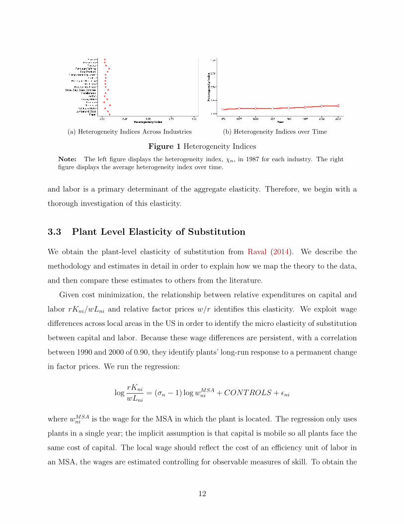
Given cost minimization, the relationship between relative expenditures on capital and
labor rKni/wLni and relative factor prices w/r identifies this elasticity. We exploit wage
differences across local areas in the US in order to identify the micro elasticity of substitution
between capital and labor. Because these wage differences are persistent, with a correlation
between 1990 and 2000 of 0.90, they identify plants’ long-run response to a permanent change
in factor prices. We run the regression:
logrKni
wLni= (σn − 1) logwMSA
ni + CONTROLS + εni
where wMSAni is the wage for the MSA in which the plant is located. The regression only uses
plants in a single year; the implicit assumption is that capital is mobile so all plants face the
same cost of capital. The local wage should reflect the cost of an efficiency unit of labor in
an MSA, the wages are estimated controlling for observable measures of skill. To obtain the
12
MSA wages, we first use data from the Population Censuses to estimate a residual wage for
each person after controlling for education, experience, and demographics. We then average
this residual within the MSA.13 All regressions control for industry fixed effects, as well as
plant age and multi-unit status.
This specification has several attractive properties. First, the dependent variable uses a
plant’s wage bill rather than a count of employees. If employees supply efficiency units of
labor, using the wage bill automatically controls for differences in skill across workers and,
more importantly, across plants. Second, plants may find it costly to adjust capital or labor.
Deviations of a plant’s capital or labor from static cost minimization due to adjustment costs
would be in the residual, but should be orthogonal to the MSA wage. Third, the MSA wage
and plant wage bills are calculated using different data sources, so we avoid division bias
from measurement error in the wage in the dependent and independent variables.
Using all manufacturing plants, Raval (2014) estimates a plant level elasticity of substi-
tution close to one-half in both 1987 and 1997. In this paper, we allow plant elasticities
of substitution to vary by two digit SIC industry and so run separate regressions for each
industry. Figure 2 displays the estimates by industry along with 95 percent confidence in-
tervals.14 Most of the estimates range between 0.4 and 0.7. The remainder of this section
addresses a number of potential issues with our plant level elasticity estimates.
Endogeneity
We estimated the plant level elasticity of substitution using cross-sectional wage differ-
ences across US locations. A natural question is whether these wage differences are exogenous
to non-neutral productivity differences. For example, to the extent that higher MSA wages
were caused by higher labor-augmenting productivity or unobserved skills, our estimate of
the elasticity of substitution would be biased towards one as σ − 1 would be attenuated.
To address such endogeneity problems, we use a version of Bartik (1991)’s instrument for
labor demand, which is based on the premise that MSAs differ in their industrial composi-
tion. When an industry expands nationwide, MSAs more heavily exposed to that industry
experience larger increases in labor demand. Thus given each MSA’s initial industrial com-
13For details about how we construct this wage, see Web Appendix C.2.14We list these estimates in Web Appendix D.1.
13
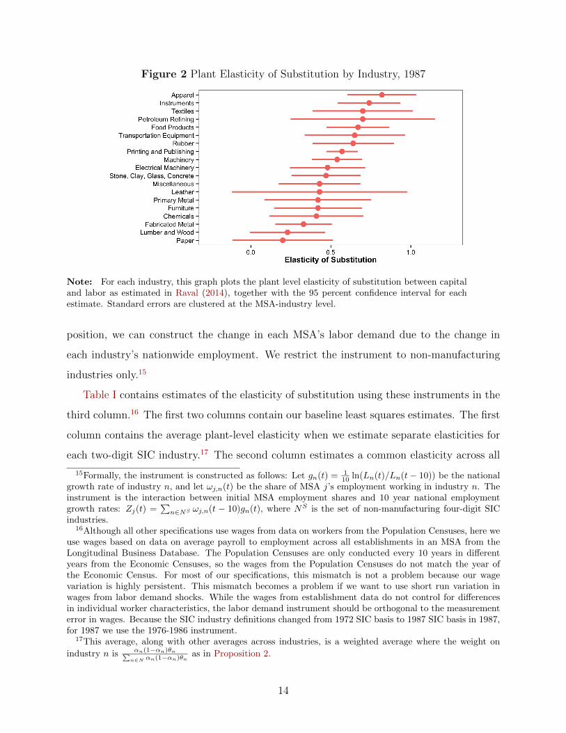
Figure 2 Plant Elasticity of Substitution by Industry, 1987
Note: For each industry, this graph plots the plant level elasticity of substitution between capitaland labor as estimated in Raval (2014), together with the 95 percent confidence interval for eachestimate. Standard errors are clustered at the MSA-industry level.
position, we can construct the change in each MSA’s labor demand due to the change in
each industry’s nationwide employment. We restrict the instrument to non-manufacturing
industries only.15
Table I contains estimates of the elasticity of substitution using these instruments in the
third column.16 The first two columns contain our baseline least squares estimates. The first
column contains the average plant-level elasticity when we estimate separate elasticities for
each two-digit SIC industry.17 The second column estimates a common elasticity across all
15Formally, the instrument is constructed as follows: Let gn(t) = 110 ln(Ln(t)/Ln(t− 10)) be the national
growth rate of industry n, and let ωj,n(t) be the share of MSA j’s employment working in industry n. Theinstrument is the interaction between initial MSA employment shares and 10 year national employmentgrowth rates: Zj(t) =
∑n∈NS ωj,n(t − 10)gn(t), where NS is the set of non-manufacturing four-digit SIC
industries.16Although all other specifications use wages from data on workers from the Population Censuses, here we
use wages based on data on average payroll to employment across all establishments in an MSA from theLongitudinal Business Database. The Population Censuses are only conducted every 10 years in differentyears from the Economic Censuses, so the wages from the Population Censuses do not match the year ofthe Economic Census. For most of our specifications, this mismatch is not a problem because our wagevariation is highly persistent. This mismatch becomes a problem if we want to use short run variation inwages from labor demand shocks. While the wages from establishment data do not control for differencesin individual worker characteristics, the labor demand instrument should be orthogonal to the measurementerror in wages. Because the SIC industry definitions changed from 1972 SIC basis to 1987 SIC basis in 1987,for 1987 we use the 1976-1986 instrument.
17This average, along with other averages across industries, is a weighted average where the weight on
industry n is αn(1−αn)θn∑n∈N αn(1−αn)θn as in Proposition 2.
14
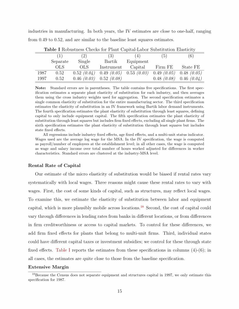
industries in manufacturing. In both years, the IV estimates are close to one-half, ranging
from 0.49 to 0.52, and are similar to the baseline least squares estimates.
Table I Robustness Checks for Plant Capital-Labor Substitution Elasticity
(1) (2) (3) (4) (5) (6)Separate Single Bartik Equipment
OLS OLS Instrument Capital Firm FE State FE1987 0.52 0.52 (0.04) 0.49 (0.05) 0.53 (0.03) 0.49 (0.05) 0.48 (0.05)1997 0.52 0.46 (0.03) 0.52 (0.08) 0.48 (0.08) 0.46 (0.04)
Note: Standard errors are in parentheses. The table contains five specifications. The first spec-ification estimates a separate plant elasticity of substitution for each industry, and then averagesthem using the cross industry weights used for aggregation. The second specification estimates asingle common elasticity of substitution for the entire manufacturing sector. The third specificationestimates the elasticity of substitution in an IV framework using Bartik labor demand instruments.The fourth specification estimates the plant elasticity of substitution through least squares, definingcapital to only include equipment capital. The fifth specification estimates the plant elasticity ofsubstitution through least squares but includes firm fixed effects, excluding all single plant firms. Thesixth specification estimates the plant elasticity of substitution through least squares but includesstate fixed effects.
All regressions include industry fixed effects, age fixed effects, and a multi-unit status indicator.Wages used are the average log wage for the MSA. In the IV specification, the wage is computedas payroll/number of employees at the establishment level; in all other cases, the wage is computedas wage and salary income over total number of hours worked adjusted for differences in workercharacteristics. Standard errors are clustered at the industry-MSA level.
Rental Rate of Capital
Our estimate of the micro elasticity of substitution would be biased if rental rates vary
systematically with local wages. Three reasons might cause these rental rates to vary with
wages. First, the cost of some kinds of capital, such as structures, may reflect local wages.
To examine this, we estimate the elasticity of substitution between labor and equipment
capital, which is more plausibly mobile across locations.18 Second, the cost of capital could
vary through differences in lending rates from banks in different locations, or from differences
in firm creditworthiness or access to capital markets. To control for these differences, we
add firm fixed effects for plants that belong to multi-unit firms. Third, individual states
could have different capital taxes or investment subsidies; we control for these through state
fixed effects. Table I reports the estimates from these specifications in columns (4)-(6); in
all cases, the estimates are quite close to those from the baseline specification.
Extensive Margin
18Because the Census does not separate equipment and structures capital in 1997, we only estimate thisspecification for 1987.
15
In the baseline model presented in Section 2, plants could substitute across inputs and
change size. However, the set of existing plants remained fixed, so there was no extensive
margin of adjustment. Would a higher wage cause entering firms to choose more capital
intensive technologies? If so, the aggregate elasticity of substitution should account for that
shift.
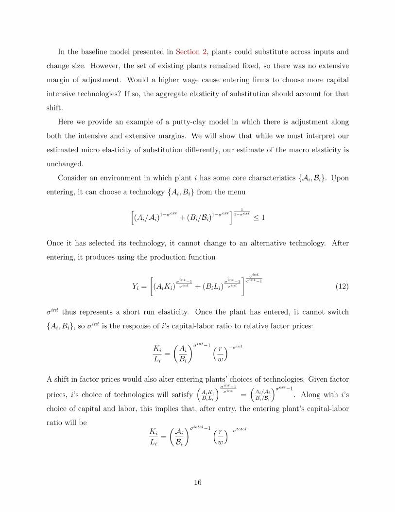
Here we provide an example of a putty-clay model in which there is adjustment along
both the intensive and extensive margins. We will show that while we must interpret our
estimated micro elasticity of substitution differently, our estimate of the macro elasticity is
unchanged.
Consider an environment in which plant i has some core characteristics {Ai,Bi}. Upon
entering, it can choose a technology {Ai, Bi} from the menu
[(Ai/Ai)1−σ
ext
+ (Bi/Bi)1−σext] 1
1−σext ≤ 1
Once it has selected its technology, it cannot change to an alternative technology. After
entering, it produces using the production function
Yi =
[(AiKi)
σint−1
σint + (BiLi)σint−1
σint
] σint
σint−1
(12)
σint thus represents a short run elasticity. Once the plant has entered, it cannot switch
{Ai, Bi}, so σint is the response of i’s capital-labor ratio to relative factor prices:
Ki
Li=
(AiBi
)σint−1 ( rw
)−σintA shift in factor prices would also alter entering plants’ choices of technologies. Given factor
prices, i’s choice of technologies will satisfy(AiKiBiLi
)σint−1
σint
=(Ai/AiBi/Bi
)σext−1. Along with i’s
choice of capital and labor, this implies that, after entry, the entering plant’s capital-labor
ratio will beKi
Li=
(AiBi
)σtotal−1 ( rw
)−σtotal
16
where σtotal is defined to satisfy
1
σtotal − 1=
1
σint − 1+
1
σext − 1
σtotal represents a long run elasticity of substitution. If, for example, the wage was high
and remained high, all entering plants would choose more capital intensive technologies, and
σtotal would capture the resulting shifts in capital-labor ratios.
If the true model contains both an intensive and extensive margin, then how should we
interpret our estimates of the micro elasticity? Our estimation strategy uses cross-sectional
differences; we compare capital-labor ratios across locations with different wages. These
differences in capital-labor ratios come from some combination of the intensive and extensive
margins. Because geographic wage differences are extremely persistent, our estimated micro
elasticity corresponds to σtotal; in high-wage locations, past entering cohorts would have
selected technologies that reflected the higher cost of labor.
With our methodology we are unable to distinguish between the intensive and extensive
margins of adjustment. Fortunately, doing so is not necessary to build up to a long-run
aggregate elasticity.19
Sorting
Our estimates do not account for the possibility that plants select locations in response
to factor prices. To see why this might matter, consider the following extreme example:
Suppose plants cannot adjust their factor usage but can move freely. Then we would expect
to find more labor intensive plants in locations with lower wages. A national increase in the
wage would not, however, change any plant’s factor usage. Thus, to the extent that this
channel is important, our estimated elasticity will overstate the true elasticity.
19Houthakker (1955) also features an extensive margin. We do not have a general result for that type ofenvironment, but we can show that under his assumptions our methodology would deliver an estimate of theaggregate elasticity of substitution of one. The argument that our estimated micro elasticity captures boththe intensive and extensive margins of adjustment is the same, but the mapping from Houthakker’s modelto our parameter estimates is more opaque. In that model, even though individual plants have Leontiefproduction functions, one can show that the equilibrium distribution of capital shares (αi) in the crosssection is independent of factor prices. Thus we would estimate a unit plant-level elasticity of substitution.Houthakker also assumed that each plant’s capacity was constrained by a fixed factor. This, in combinationwith his distributional assumptions, implies that the average revenue-cost ratio in that model is infinite.Thus we would estimate a unit demand elasticity (see Section 3.4). Thus, for any heterogeneity index, ourestimation strategy would yield a Cobb-Douglas aggregate production function.
17
Plants ability to sort across locations likely varies by industry. We would expect industries
in which plants are more mobile to be more clustered in particular areas. This could depend,
for example, on how easily goods can be shipped to other locations.
Raval (2014) addressed this by looking at a set of ten large four-digit industries located
in almost all MSAs and states. These are industries for which we would expect sorting across
locations to be least important. The leading example of this is ready-mixed concrete; because
concrete cannot be shipped very far, concrete plants exist in every locality. Elasticities for
these industries are similar to the estimates for all industries in our baseline, with average
elasticities of 0.49 for 1987 and 0.61 for 1997.
Alternative Estimates
Our estimation strategy uses cross-sectional variation to estimate a long-run plant-level
elasticity. Chirinko (2008) surveyed the existing literature estimating short- and long-run
elasticities of substitution at various levels of aggregation. This literature typically uses
variation in the user cost of capital over time stemming from changes in tax-laws or the
price of capital that differentially affect asset types.
Chirinko et al. (2011) and Barnes et al. (2008) provided estimates that are conceptually
closest to ours, as they used long-run movements in the user cost of capital to identify the
long-run micro elasticity for US and UK public firms respectively. Their approach estimates
the elasticity using the capital first order condition and allows for biased technical change at
the industry level. Because they use variation within firms over time, their estimates are not
biased by sorting across locations. In addition, because their estimated elasticities contain
only the intensive margin of adjustment, we would expect them to be slightly lower than
ours. Each estimated a micro elasticity of substitution of 0.4. We find it comforting that
two approaches that use very different sources of variation yield similar estimates.
3.4 Aggregation
We now estimate the remaining plant-level production and demand parameters. We then
use them to aggregate to the manufacturing-level elasticity of substitution.
The reallocation effect depends upon both the plant elasticity of substitution between
materials and non-materials, ζ, and the elasticity of demand, ε.
18
To identify ζ, we use the same cross-area variation in the wage. Across MSAs, the local
wage varies but the prices of capital and materials are fixed. Cost minimization implies that
ζ measures the response of relative expenditures of materials and non-materials to changes
in their respective prices: 1 − ζ = d ln[(rKni+wLni)/qMni]d ln(λni/q)
, where λni is the cost index of i’s
capital-labor bundle. Holding fixed the prices of materials and capital, a change in the
local wage would increase these relative prices by d lnλni/q = (1 − αni)d lnwMSAni . To a
first-order approximation, the response of (rKni + wLni)/qMni to the local wage would be
(1− ζ)(1− αni). We therefore estimate ζ using the regression
logrKni + wLni
qMni
= (1− ζ)(1− αni)(logwMSAni ) + CONTROLS + εni
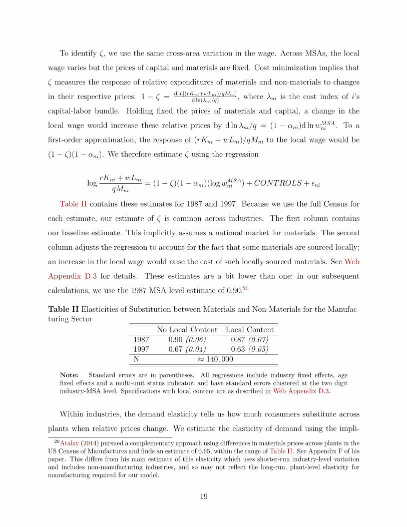
Table II contains these estimates for 1987 and 1997. Because we use the full Census for
each estimate, our estimate of ζ is common across industries. The first column contains
our baseline estimate. This implicitly assumes a national market for materials. The second
column adjusts the regression to account for the fact that some materials are sourced locally;
an increase in the local wage would raise the cost of such locally sourced materials. See Web
Appendix D.3 for details. These estimates are a bit lower than one; in our subsequent
calculations, we use the 1987 MSA level estimate of 0.90.20
Table II Elasticities of Substitution between Materials and Non-Materials for the Manufac-turing Sector
No Local Content Local Content1987 0.90 (0.06) 0.87 (0.07)1997 0.67 (0.04) 0.63 (0.05)N ≈ 140, 000
Note: Standard errors are in parentheses. All regressions include industry fixed effects, agefixed effects and a multi-unit status indicator, and have standard errors clustered at the two digitindustry-MSA level. Specifications with local content are as described in Web Appendix D.3.
Within industries, the demand elasticity tells us how much consumers substitute across
plants when relative prices change. We estimate the elasticity of demand using the impli-
20Atalay (2014) pursued a complementary approach using differences in materials prices across plants in theUS Census of Manufactures and finds an estimate of 0.65, within the range of Table II. See Appendix F of hispaper. This differs from his main estimate of this elasticity which uses shorter-run industry-level variationand includes non-manufacturing industries, and so may not reflect the long-run, plant-level elasticity formanufacturing required for our model.
19
cations of profit maximization; optimal price setting behavior implies that the markup over
marginal cost is equal to εε−1 . Thus, we invert the average markup across plants in an indus-
try to obtain the elasticity of demand. The assumption of constant returns to scale implies
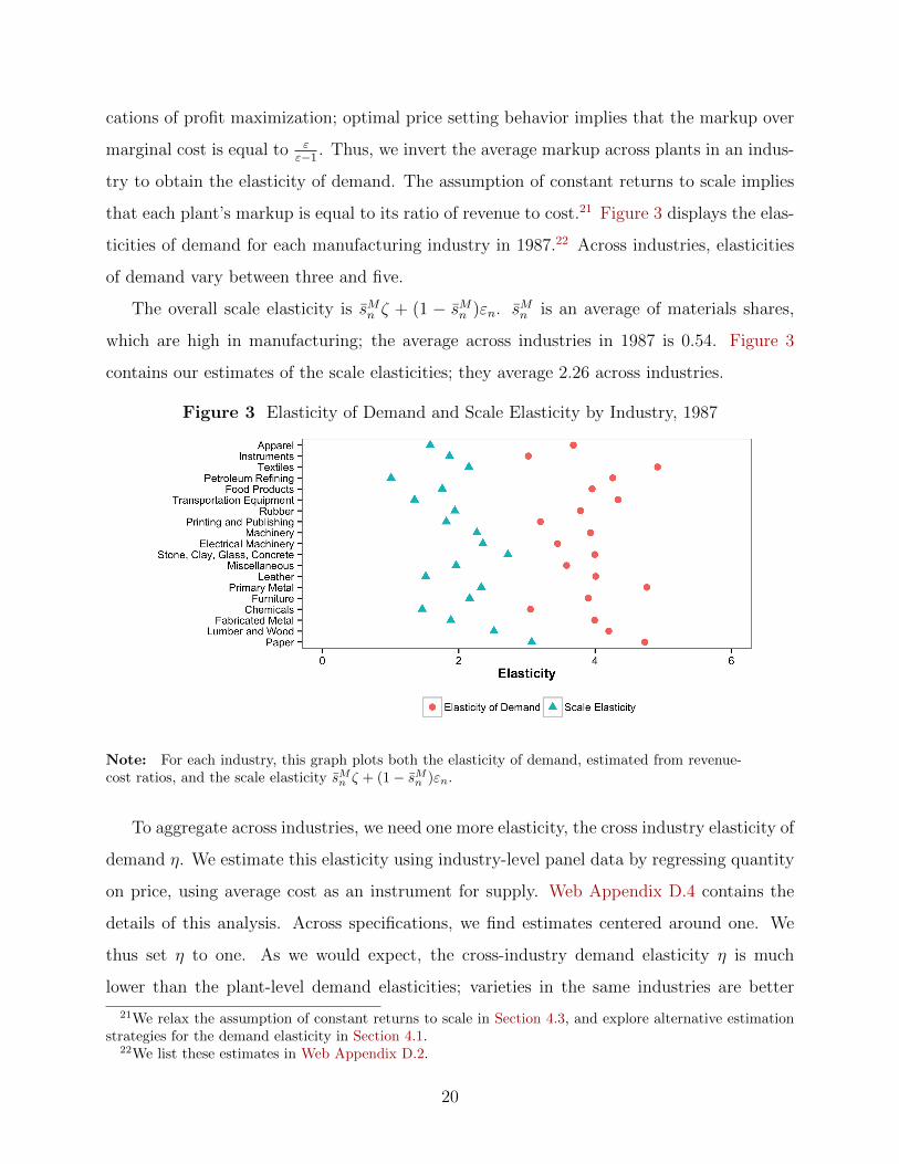
that each plant’s markup is equal to its ratio of revenue to cost.21 Figure 3 displays the elas-
ticities of demand for each manufacturing industry in 1987.22 Across industries, elasticities
of demand vary between three and five.
The overall scale elasticity is s̄Mn ζ + (1 − s̄Mn )εn. s̄Mn is an average of materials shares,
which are high in manufacturing; the average across industries in 1987 is 0.54. Figure 3
contains our estimates of the scale elasticities; they average 2.26 across industries.
Figure 3 Elasticity of Demand and Scale Elasticity by Industry, 1987
Note: For each industry, this graph plots both the elasticity of demand, estimated from revenue-cost ratios, and the scale elasticity s̄Mn ζ + (1− s̄Mn )εn.
To aggregate across industries, we need one more elasticity, the cross industry elasticity of
demand η. We estimate this elasticity using industry-level panel data by regressing quantity
on price, using average cost as an instrument for supply. Web Appendix D.4 contains the
details of this analysis. Across specifications, we find estimates centered around one. We
thus set η to one. As we would expect, the cross-industry demand elasticity η is much
lower than the plant-level demand elasticities; varieties in the same industries are better
21We relax the assumption of constant returns to scale in Section 4.3, and explore alternative estimationstrategies for the demand elasticity in Section 4.1.
22We list these estimates in Web Appendix D.2.
20
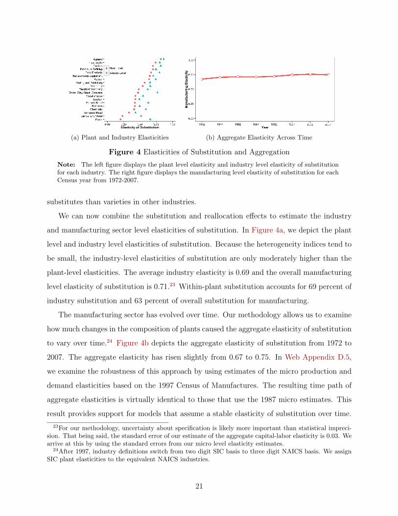
(a) Plant and Industry Elasticities (b) Aggregate Elasticity Across Time
Figure 4 Elasticities of Substitution and Aggregation
Note: The left figure displays the plant level elasticity and industry level elasticity of substitutionfor each industry. The right figure displays the manufacturing level elasticity of substitution for eachCensus year from 1972-2007.
substitutes than varieties in other industries.
We can now combine the substitution and reallocation effects to estimate the industry
and manufacturing sector level elasticities of substitution. In Figure 4a, we depict the plant
level and industry level elasticities of substitution. Because the heterogeneity indices tend to
be small, the industry-level elasticities of substitution are only moderately higher than the
plant-level elasticities. The average industry elasticity is 0.69 and the overall manufacturing
level elasticity of substitution is 0.71.23 Within-plant substitution accounts for 69 percent of
industry substitution and 63 percent of overall substitution for manufacturing.
The manufacturing sector has evolved over time. Our methodology allows us to examine
how much changes in the composition of plants caused the aggregate elasticity of substitution
to vary over time.24 Figure 4b depicts the aggregate elasticity of substitution from 1972 to
2007. The aggregate elasticity has risen slightly from 0.67 to 0.75. In Web Appendix D.5,
we examine the robustness of this approach by using estimates of the micro production and
demand elasticities based on the 1997 Census of Manufactures. The resulting time path of
aggregate elasticities is virtually identical to those that use the 1987 micro estimates. This
result provides support for models that assume a stable elasticity of substitution over time.
23For our methodology, uncertainty about specification is likely more important than statistical impreci-sion. That being said, the standard error of our estimate of the aggregate capital-labor elasticity is 0.03. Wearrive at this by using the standard errors from our micro level elasticity estimates.
24After 1997, industry definitions switch from two digit SIC basis to three digit NAICS basis. We assignSIC plant elasticities to the equivalent NAICS industries.
21
4 Robustness
In this section, we examine the robustness and sensitivity of our estimates to alternative
modeling assumptions. We first examine our estimates of the micro elasticities of demand.
We also discuss measurement error and changes in the specification of the economic envi-
ronment, including imperfect pass-through, returns to scale, adjustment costs, and other
misallocation frictions.
4.1 Elasticity of Demand
For several homogeneous products, the US Census of Manufactures collects both price and
physical quantity data. We can thus estimate the elasticity of demand by regressing quantity
on price, instrumenting for price using average cost. This approach is similar to Foster et al.
(2008). This strategy implies an average industry-level capital-labor elasticity of substitution
of 0.52 among these industries, close to the estimate of 0.54 using our baseline strategy.25
The trade literature finds estimates in the same range using within industry variation across
imported varieties to identify the elasticity of demand. For example, Imbs and Mejean (2011)
find a median elasticity of 4.1 across manufacturing industries.
Web Appendix B.5 generalizes the analysis to a homothetic demand system with arbitrary
demand elasticities and imperfect pass-through of marginal cost. In that environment, the
formula for the industry elasticity in Proposition 1 is unchanged except the elasticity of
demand εn is replaced by a weighted average of the quantity bniεni; εni is i’s local demand
elasticity and bni is i’s local rate of relative pass-through (the elasticity of its price to a change
in marginal cost). Note that under Dixit-Stiglitz preferences, bni = 1 and εni = εn for each
i. Here, however, if a plant passes through only three-quarters of a marginal cost increase,
then the subsequent change in scale would be three-quarters as large. Given a pass-through
rate of three-quarters, our estimate of the 1987 aggregate elasticity of substitution would be
25Foster et al. (2008) instrument for price using plant-level TFP. We cannot use their estimates directlybecause they assume plants produce using homogeneous Cobb-Douglas production functions. Because wemaintain the assumption of constant returns to scale, the appropriate analogue to plant-level TFP is averagecost. Directly using the demand elasticities of Foster et al. (2008) would yield an average industry-levelelasticity of substitution of 0.54.
22
0.67.
4.2 Non-CES Production Functions
In our baseline model, we assumed that within an industry, each plant produced using a
nested CES production function with common elasticities. Here we relax the strong func-
tional form assumption. While we maintain that each plant’s production function has con-
stant returns to scale, we impose no further structure. In particular, we do not assume
substitution elasticities are constant, that inputs are separable, or that technological differ-
ences across plants are factor augmenting. Rather, we relate the industry-level elasticity of
substitution to local elasticities of individual plants.
For plant i, we define the local elasticities σni and ζni to satisfy σni − 1 ≡ d ln rKni/wLnid lnw/r
and ζni− 1 ≡ 1αM−αni
d lnqMni
rKni+wLni
d lnw/r.26 In Appendix A we derive an expression for the industry
elasticity of substitution in this environment. The resulting expression is identical to Propo-
sition 1 except the plant elasticities of substitution are replaced with weighted averages of the
plants’ local elasticities, σ̄n ≡∑
i∈Inαni(1−αni)θni∑
i′∈In αni′ (1−αni′ )θni′σni and ζ̄n ≡
∑i∈In
(αni−αn)(αni−αM )sMni∑i′∈In (αni′−αn)(αni′−α
M )sMi′ζni:
σNn = (1− χn)σ̄n + χn[(1− s̄n)εn + s̄Mn ζ̄n
]4.3 Returns to Scale
Our baseline estimation assumed that each plant produced using a production function with
constant returns to scale. Alternatively, we can assume that plant i produces using the
production function:
Yni = Fni(Kni, Lni,Mni) = Gni(Kni, Lni,Mni)γ
26If i’s production function takes a nested CES form as in Assumption 1, σni and ζni would equal σn andζn respectively. The definition of σni is straightforward but ζni is more subtle; see Appendix A for details.Here, however, these elasticities are not parameters of a production function. Instead, they are definedlocally in terms of derivatives of i’s production function evaluated at the cost-minimizing input bundle.Exact expressions for σni and ζni are given in Web Appendix B.1.
23
where Gni has constant returns to scale and γ < εnεn−1 . Relative to the baseline, two things
change, as shown in Web Appendix B.3. First, the industry elasticity of substitution becomes
σNn = (1− χn)σ̄n + χn[s̄Mn ζ̄n + (1− s̄Mn )xn
]where xn is defined to satisfy xn
xn−1 = 1γ
εnεn−1 . Thus the scale elasticity is a composite of two
parameters, the elasticity of demand and the returns to scale. When the wage falls, the
amount a labor-intensive plant would expand depends on both.
Second, when we divide a plant’s revenue by total cost, we no longer recover the markup.
Instead, we getPniYni
rKni + wLni + qMni
=1
γ
εnεn − 1
=xn
xn − 1
Fortunately, this means that the procedure we used in the baseline delivers the correct
aggregate elasticity of substitution even if we mis-specify the returns to scale. To see this,
when we assumed constant returns to scale, we found the elasticity of demand by computingPniYni
rKni+wLni+qMniPniYni
rKni+wLni+qMni−1
. With alternative returns to scale, this would no longer give the elasticity
of demand, εn; rather, it gives the correct scale elasticity, xn.27
4.4 Adjustment Costs and Distortions
Section 2 showed that the relative importance of within-plant substitution and reallocation
depends upon the variation in cost shares of capital. Implicit in that environment was that
this variation came from non-neutral differences in technology. On the other hand, some
of this heterogeneity may be due to adjustment costs or other distortions as in the recent
misallocation literature; see Banerjee and Duflo (2005), Restuccia and Rogerson (2008),
Hsieh and Klenow (2009). A natural question arises: What are the implications for the
aggregate elasticity of substitution if these differences come from distortions?
Consider an alternative environment in which plants pay idiosyncratic prices for their
27This specification of returns to scale rules out some features such as fixed costs of production. In anenvironment in which production functions exhibited such features, xn would be replaced by a weightedaverage of individual plants’ local scale elasticities. For details see Web Appendix B.6, which also derives anaggregate elasticity when production functions are non-homothetic.
24
inputs.28 We are interested in how changes in factor prices impact the relative compensation
of capital and labor. To be precise, suppose plant i pays factor prices rni = TKnir and
wni = TLniw, and we define the industry elasticity of substitution in relation to the change
in relative factor compensation in response to a change in w/r (holding fixed the idiosyncratic
components of factor prices, {TKni, TLni}i∈In) so that it satisfies29
σNn − 1 =d ln
(∑i∈In rniKni/
∑i∈In wniLni
)d lnw/r
As shown in Web Appendix B.4, it turns out that the expression for the industry elasticity
of substitution is exactly the same as in Proposition 1, provided that we define αi = riKiriKi+wiLi
and θi = rniKni+wniLni∑i′∈In rni′Kni′+wni′Lni′
. Thus, as long as expenditures are measured correctly, no
modifications are necessary.
Alternatively, a plant’s shadow value of an input may differ from its marginal expenditure
on that input. This could happen if the input is fixed in the short run or if use of that input
is constrained by something other than prices. In the presence of such “unpaid” wedges, our
expression for the industry elasticity would change slightly.
If we observed these unpaid wedges, we could compute the industry elasticity. However,
measuring these wedges presents a challenge. Differences in plants’ cost shares of capital
could reflect differences in unpaid wedges or differences in technology; data on revenue and
input expenditures alone are not sufficient to distinguish between the two.
To get a sense of how big of an issue these unpaid wedges might represent, we consider
the following thought experiment. Suppose all variation in cost shares of capital were due to
“unpaid” wedges. In that case, the aggregate elasticity of substitution for the manufacturing
sector in 1987 would be 0.71, the same as our baseline, while in 1997 the aggregate elasticity
would be 0.91 rather than 0.75 in the baseline (see Web Appendix B.4 for details). This
suggests that misallocation would not substantially alter our analysis.
28In fact, our identification of the plant-level elasticity of substitution relies on plants (in different locations)facing different wages.
29In this environment the mapping between changes in the capital-labor ratio and changes in factor com-
pensation is fuzzy; generically, d lnKn/Lnd lnw/r − 1 6= d ln
∑i∈In rniKni/
∑i∈In wniLni
d lnw/r .
25
4.5 Measurement Error
The measured heterogeneity indices may be affected by measurement error. Two types of
measurement error might play a role. First, if the costs of capital or labor are misreported
or constructed incorrectly, we would likely overstate the heterogeneity indices as they would
include both true heterogeneity and measurement error. In the extreme case in which all
measured heterogeneity reflects mismeasurement, then the true aggregate elasticity would
equal the plant-level elasticity. A second type of measurement error would work in the op-
posite direction. As described by White et al. (2012), data for some plants in the Census are
imputed, reducing the measured dispersion of productivity. This means that our measured
heterogeneity indices might understate the true heterogeneity in capital intensities.
A reason to think measurement error might not play a big role is that both types of
measurement discussed above are much more important for small plants than for large plants,
and the heterogeneity indices are weighted by expenditure.
5 The Decline of the Labor Share
Figure 5 depicts the labor share of income in the US for the manufacturing sector and for the
aggregate economy in the post-war period.30 The labor share for manufacturing has fallen
since 1970, from about 0.73 to 0.55 in 2011. The steepest decline has been since 2000; the
labor share fell from roughly 0.65 to 0.55 in one decade. The labor share has fallen for the
overall economy as well, though not by as much, falling from 0.70 in 1970 to 0.62 in 2011.
Labor’s share of income could change in response to factor prices or for other reasons
which, through the lens of an aggregate production function, would be viewed as biased
technical change. The aggregate elasticity determines the impact of changes in factor prices;
30The labor share for manufacturing comes from the BLS Multifactor Productivity Series, while theaggregate labor share comes from Fernald (2012); both are based on data from the National Accounts. AsGomme and Rupert (2004), Krueger (1999), and Elsby et al. (2013) point out, the major issue with calculatingthe labor share is whether proprietors’ income accrues to labor or capital. Both series assume that the shareof labor for proprietors is the same as for corporations. For the manufacturing sector, proprietors’ incomerepresented 1.4 percent of income on average since 1970. Industry definitions change over this period fromSIC basis to NAICS basis; for consistency, we include NAICS Publishing Industries in manufacturing becausePublishing was included in manufacturing on a SIC basis.
26
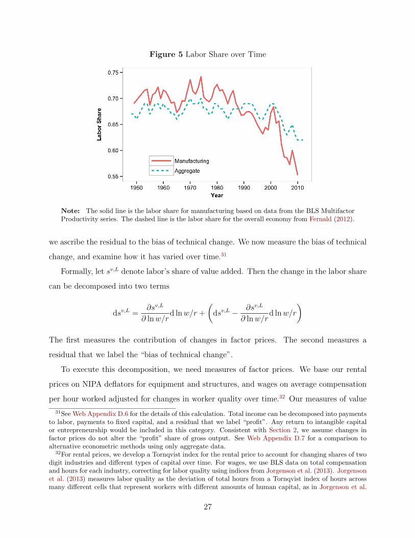
Figure 5 Labor Share over Time
Note: The solid line is the labor share for manufacturing based on data from the BLS MultifactorProductivity series. The dashed line is the labor share for the overall economy from Fernald (2012).
we ascribe the residual to the bias of technical change. We now measure the bias of technical
change, and examine how it has varied over time.31
Formally, let sv,L denote labor’s share of value added. Then the change in the labor share
can be decomposed into two terms
dsv,L =∂sv,L
∂ lnw/rd lnw/r +
(dsv,L − ∂sv,L
∂ lnw/rd lnw/r
)
The first measures the contribution of changes in factor prices. The second measures a
residual that we label the “bias of technical change”.
To execute this decomposition, we need measures of factor prices. We base our rental
prices on NIPA deflators for equipment and structures, and wages on average compensation
per hour worked adjusted for changes in worker quality over time.32 Our measures of value
31See Web Appendix D.6 for the details of this calculation. Total income can be decomposed into paymentsto labor, payments to fixed capital, and a residual that we label “profit”. Any return to intangible capitalor entrepreneurship would be included in this category. Consistent with Section 2, we assume changes infactor prices do not alter the “profit” share of gross output. See Web Appendix D.7 for a comparison toalternative econometric methods using only aggregate data.
32For rental prices, we develop a Tornqvist index for the rental price to account for changing shares of twodigit industries and different types of capital over time. For wages, we use BLS data on total compensationand hours for each industry, correcting for labor quality using indices from Jorgenson et al. (2013). Jorgensonet al. (2013) measures labor quality as the deviation of total hours from a Tornqvist index of hours acrossmany different cells that represent workers with different amounts of human capital, as in Jorgenson et al.
27
added and input expenditures are based on NIPA data. Our estimates of expenditures
on fixed capital combine NIPA data on equipment and structures capital with our rental
prices.33 Finally, we allow the aggregate elasticity to vary across time, linearly interpolating
between the Census years in which we estimated the elasticity.
Table III displays the annualized change in the labor share and each of its components
before and after the year 2000. This type of decomposition cannot provide a full explanation
of the decline in the labor share. Nevertheless, any explanation should be consistent with
the patterns that we depict.
We have several findings. First, an estimated aggregate elasticity less than one implies
that two mechanisms that have been put forward – an acceleration in investment specific
technical change as in Karabarbounis and Neiman (2014) or increased capital accumulation
as in Piketty (2014) – would have raised rather than lowered labor’s share of income. The
declining cost of capital relative to labor raised the labor share by a total of 3.2 percentage
points over the 1970-2010 period.34 Second, the contribution of changes in factor prices has
been relatively constant over the past 40 years, at 0.08 percentage points per year in the
1970-1999 period and 0.07 percentage points per year in the 2000-2010 period. This means
that other explanations that work through factor prices, such as a decline in labor supplied
by prime-aged males or changes in benefits, would have trouble matching the timing of the
decline in the labor share.
Instead, there has been an acceleration in the bias of technical change over the past 40
years; the labor share has decreased about half a percentage point faster in the period since
(2005).33The labor share from NIPA is based on firm level data, rather than production level data, and so would
include non-manufacturing establishments of a manufacturing firm, such as a firm’s headquarters. In 1987,the total wages and salaries from the production data (from the NBER-CES Productivity database) was88.2 percent of the wages and salaries from NIPA. While our aggregate elasticities are estimated usingproduction data, we apply these elasticities to labor shares from NIPA. This is our preferred estimate. SeeWeb Appendix D.6.2 for details and alternative measures.
34Our rental prices are based upon official NIPA deflators for equipment and structures capital. However,Gordon (1990) has argued that the NIPA deflators underestimate the actual fall in equipment prices overtime. In Web Appendix D.6.3 we use an alternative rental price series for equipment capital that Cumminsand Violante (2002) developed by extending the work of Gordon (1990). Their series extends to 1999, so wecompare our baseline to these rental prices during the 1970-1999 period. Using the Cummins and Violante(2002) equipment prices implies that the wage to rental price ratio has increased by 3.8 percent per year,instead of 2.0 percent per year with the NIPA deflators. This change increases the contribution of factorprices to the labor share between 1970 and 1999 by 0.05 percentage points per year, or about 1.9 percentagepoints over the period.
28
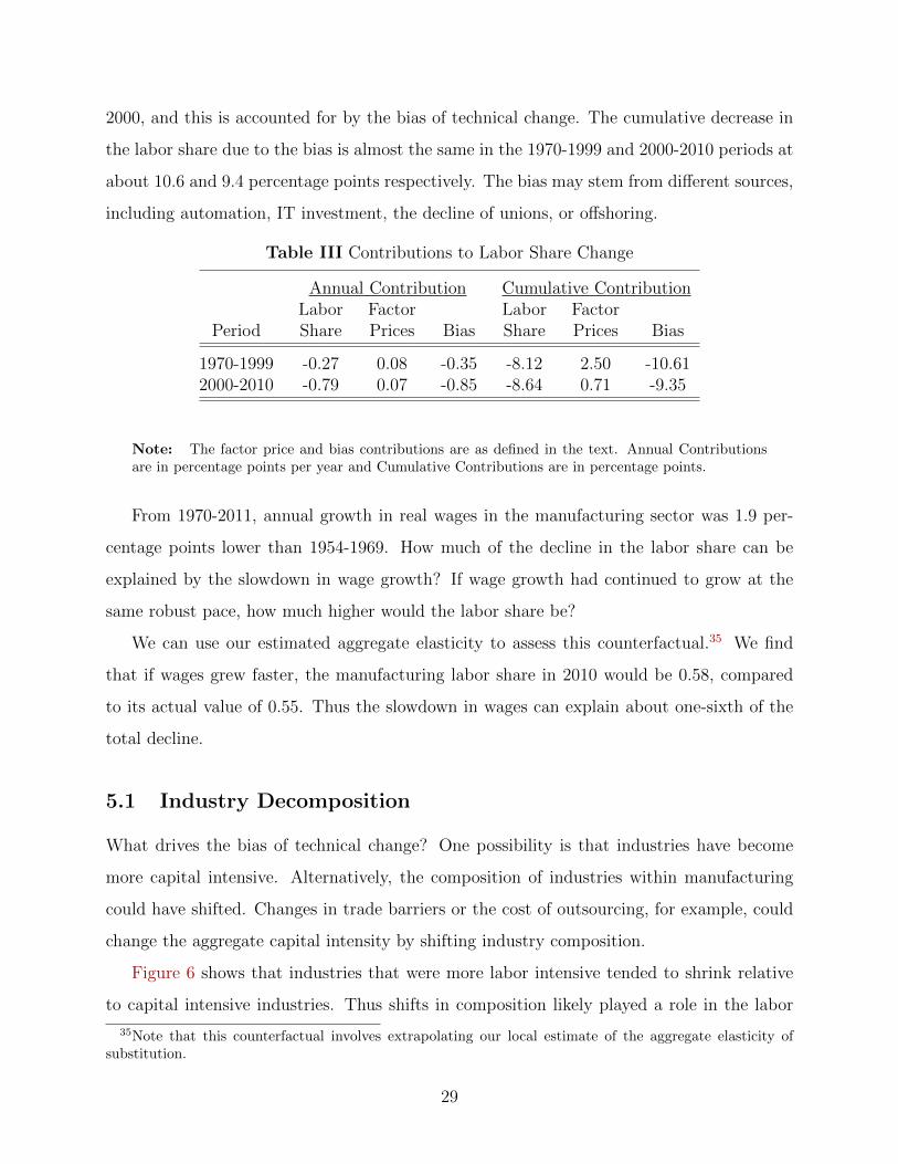
2000, and this is accounted for by the bias of technical change. The cumulative decrease in
the labor share due to the bias is almost the same in the 1970-1999 and 2000-2010 periods at
about 10.6 and 9.4 percentage points respectively. The bias may stem from different sources,
including automation, IT investment, the decline of unions, or offshoring.
Table III Contributions to Labor Share Change
Annual Contribution Cumulative ContributionLabor Factor Labor Factor
Period Share Prices Bias Share Prices Bias
1970-1999 -0.27 0.08 -0.35 -8.12 2.50 -10.612000-2010 -0.79 0.07 -0.85 -8.64 0.71 -9.35
Note: The factor price and bias contributions are as defined in the text. Annual Contributionsare in percentage points per year and Cumulative Contributions are in percentage points.
From 1970-2011, annual growth in real wages in the manufacturing sector was 1.9 per-
centage points lower than 1954-1969. How much of the decline in the labor share can be
explained by the slowdown in wage growth? If wage growth had continued to grow at the
same robust pace, how much higher would the labor share be?
We can use our estimated aggregate elasticity to assess this counterfactual.35 We find
that if wages grew faster, the manufacturing labor share in 2010 would be 0.58, compared
to its actual value of 0.55. Thus the slowdown in wages can explain about one-sixth of the
total decline.
5.1 Industry Decomposition
What drives the bias of technical change? One possibility is that industries have become
more capital intensive. Alternatively, the composition of industries within manufacturing
could have shifted. Changes in trade barriers or the cost of outsourcing, for example, could
change the aggregate capital intensity by shifting industry composition.
Figure 6 shows that industries that were more labor intensive tended to shrink relative
to capital intensive industries. Thus shifts in composition likely played a role in the labor
35Note that this counterfactual involves extrapolating our local estimate of the aggregate elasticity ofsubstitution.
29
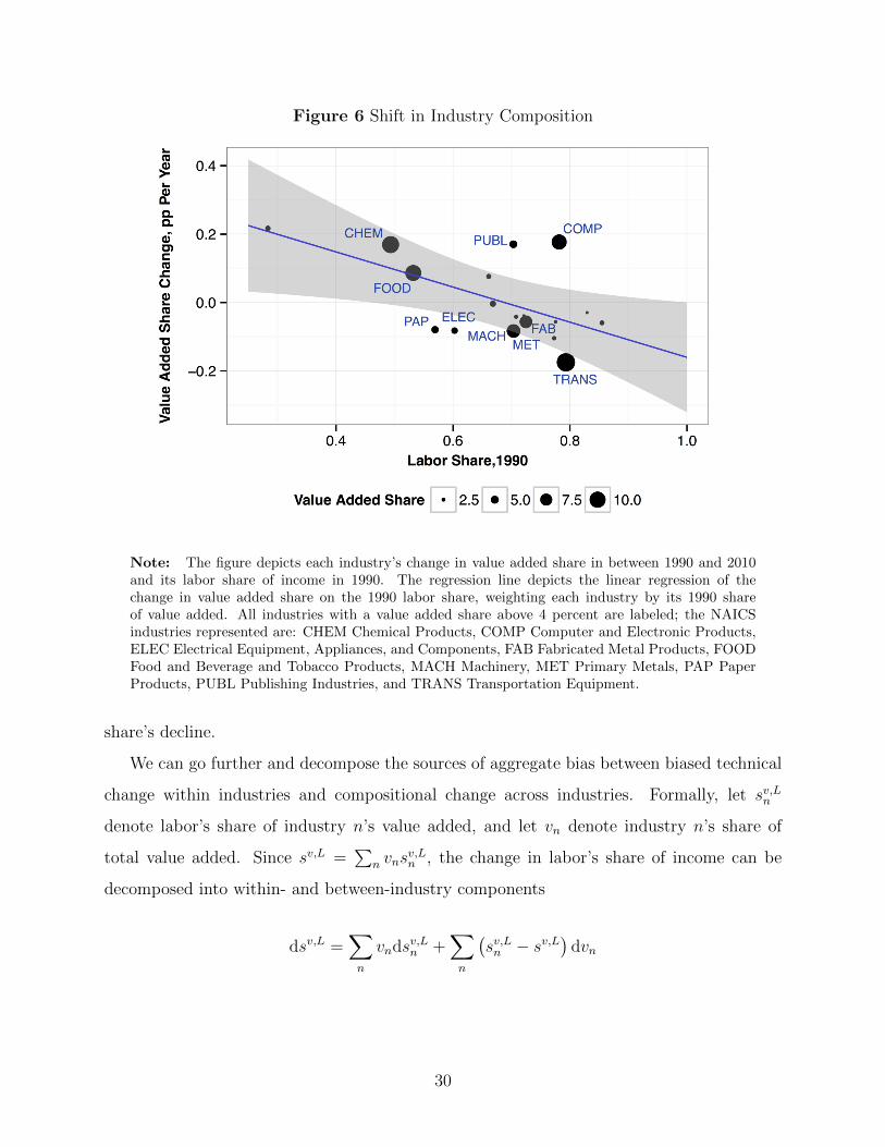
Figure 6 Shift in Industry Composition
Note: The figure depicts each industry’s change in value added share in between 1990 and 2010and its labor share of income in 1990. The regression line depicts the linear regression of thechange in value added share on the 1990 labor share, weighting each industry by its 1990 shareof value added. All industries with a value added share above 4 percent are labeled; the NAICSindustries represented are: CHEM Chemical Products, COMP Computer and Electronic Products,ELEC Electrical Equipment, Appliances, and Components, FAB Fabricated Metal Products, FOODFood and Beverage and Tobacco Products, MACH Machinery, MET Primary Metals, PAP PaperProducts, PUBL Publishing Industries, and TRANS Transportation Equipment.
share’s decline.
We can go further and decompose the sources of aggregate bias between biased technical
change within industries and compositional change across industries. Formally, let sv,Ln
denote labor’s share of industry n’s value added, and let vn denote industry n’s share of
total value added. Since sv,L =∑
n vnsv,Ln , the change in labor’s share of income can be
decomposed into within- and between-industry components
dsv,L =∑n
vndsv,Ln +∑n
(sv,Ln − sv,L
)dvn
30
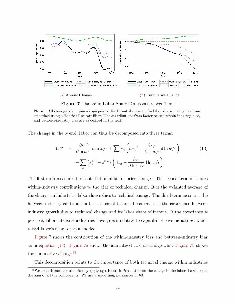
(a) Annual Change (b) Cumulative Change
Figure 7 Change in Labor Share Components over Time
Note: All changes are in percentage points. Each contribution to the labor share change has beensmoothed using a Hodrick-Prescott filter. The contributions from factor prices, within-industry bias,and between-industry bias are as defined in the text.
The change in the overall labor can thus be decomposed into three terms:
dsv,L =∂sv,L
∂ lnw/rd lnw/r +
∑n
vn
(dsv,Ln −
∂sv,Ln∂ lnw/r
d lnw/r
)(13)
+∑n
(sv,Ln − sv,L
)(dvn −
∂vn∂ lnw/r
d lnw/r
)
The first term measures the contribution of factor price changes. The second term measures
within-industry contributions to the bias of technical change. It is the weighted average of
the changes in industries’ labor shares dues to technical change. The third term measures the
between-industry contribution to the bias of technical change. It is the covariance between
industry growth due to technical change and its labor share of income. If the covariance is
positive, labor-intensive industries have grown relative to capital-intensive industries, which
raised labor’s share of value added.
Figure 7 shows the contribution of the within-industry bias and between-industry bias
as in equation (13). Figure 7a shows the annualized rate of change while Figure 7b shows
the cumulative change.36
This decomposition points to the importance of both technical change within industries
36We smooth each contribution by applying a Hodrick-Prescott filter; the change in the labor share is thenthe sum of all the components. We use a smoothing parameter of 60.
31
and compositional changes in the decline of the labor share of manufacturing. The within-
industry bias contribution has been large since the 1980s; overall, it accounts for about 12.7
percentage points of the decline in the labor share, of which about 4.4 percentage points were
in the 2000s. The between-industry bias was low for much of the sample period, but rose in
the 2000s. Overall, it accounts for about 7.2 percentage points of the decline in the labor
share, of which 4.9 percentage points were in the 2000s. The increase in the importance of
compositional change in the 2000s may point to multiple factors behind the decline in the
labor share.
Finally, we can examine how changes within industries are related to changes across
industries. Figure 8 plots each industry’s annual change in value added against the annual
change in its labor share. There was a clear shift in this relationship between the first
and second halves of the sample period. After 1990, the industries that grew more were
those with the largest decline in labor share; before 1990, the two were much less correlated.
This pattern is inconsistent with a simple story in which the labor-intensive segment of an
industry moves abroad; it is consistent with automation or a more complex offshoring story
in which both labor intensive tasks move abroad and production using capital intensive tasks
expands. The largest industries that have both expanded and become more capital intensive
are Computer Equipment and Chemicals. These industries include R&D intensive companies
such as Apple and Pfizer and may suggest the increasing importance of intangible capital.
6 Cross–Country Elasticities
How does the aggregate capital-labor elasticity vary across countries? Production technolo-
gies may differ across countries for a number of reasons. Researchers have generally found
greater variation in capital intensity and productivity in less developed countries; see Hsieh
and Klenow (2009), Bartlesman et al. (2013). This may stem from resource misallocation.
Alternatively, if lower wages in less developed countries reduce adoption of new capital inten-
sive technologies, as in Acemoglu and Zilibotti (2001), developing countries would operate
a mix of old and new technologies. In our framework, greater microeconomic heterogeneity
implies a higher aggregate capital-labor elasticity of substitution. We now examine how the
32
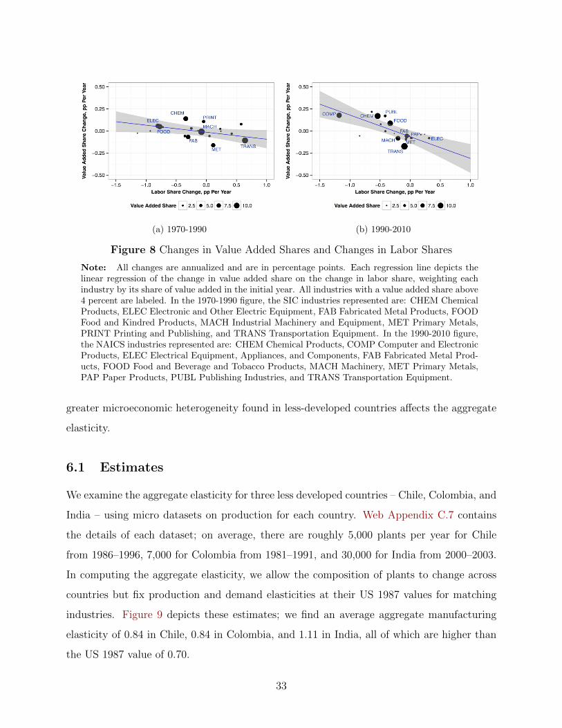
(a) 1970-1990 (b) 1990-2010
Figure 8 Changes in Value Added Shares and Changes in Labor Shares
Note: All changes are annualized and are in percentage points. Each regression line depicts thelinear regression of the change in value added share on the change in labor share, weighting eachindustry by its share of value added in the initial year. All industries with a value added share above4 percent are labeled. In the 1970-1990 figure, the SIC industries represented are: CHEM ChemicalProducts, ELEC Electronic and Other Electric Equipment, FAB Fabricated Metal Products, FOODFood and Kindred Products, MACH Industrial Machinery and Equipment, MET Primary Metals,PRINT Printing and Publishing, and TRANS Transportation Equipment. In the 1990-2010 figure,the NAICS industries represented are: CHEM Chemical Products, COMP Computer and ElectronicProducts, ELEC Electrical Equipment, Appliances, and Components, FAB Fabricated Metal Prod-ucts, FOOD Food and Beverage and Tobacco Products, MACH Machinery, MET Primary Metals,PAP Paper Products, PUBL Publishing Industries, and TRANS Transportation Equipment.
greater microeconomic heterogeneity found in less-developed countries affects the aggregate
elasticity.
6.1 Estimates
We examine the aggregate elasticity for three less developed countries – Chile, Colombia, and
India – using micro datasets on production for each country. Web Appendix C.7 contains
the details of each dataset; on average, there are roughly 5,000 plants per year for Chile
from 1986–1996, 7,000 for Colombia from 1981–1991, and 30,000 for India from 2000–2003.
In computing the aggregate elasticity, we allow the composition of plants to change across
countries but fix production and demand elasticities at their US 1987 values for matching
industries. Figure 9 depicts these estimates; we find an average aggregate manufacturing
elasticity of 0.84 in Chile, 0.84 in Colombia, and 1.11 in India, all of which are higher than
the US 1987 value of 0.70.
33
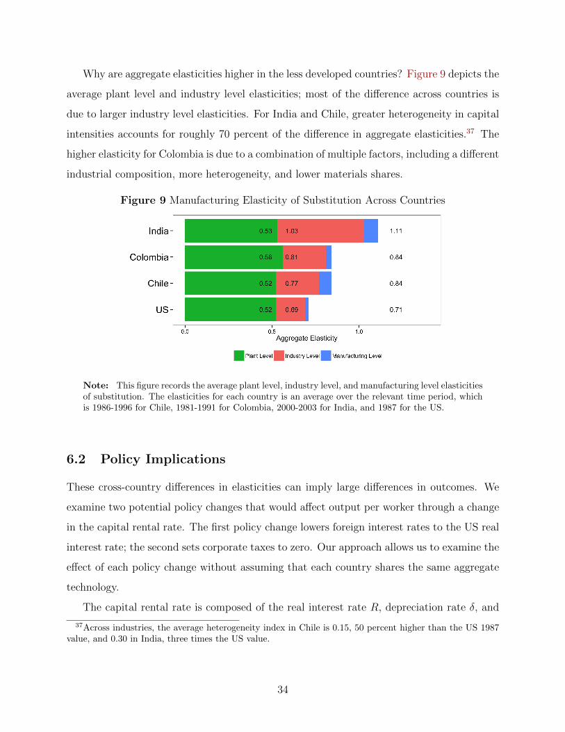
Why are aggregate elasticities higher in the less developed countries? Figure 9 depicts the
average plant level and industry level elasticities; most of the difference across countries is
due to larger industry level elasticities. For India and Chile, greater heterogeneity in capital
intensities accounts for roughly 70 percent of the difference in aggregate elasticities.37 The
higher elasticity for Colombia is due to a combination of multiple factors, including a different
industrial composition, more heterogeneity, and lower materials shares.
Figure 9 Manufacturing Elasticity of Substitution Across Countries
Note: This figure records the average plant level, industry level, and manufacturing level elasticitiesof substitution. The elasticities for each country is an average over the relevant time period, whichis 1986-1996 for Chile, 1981-1991 for Colombia, 2000-2003 for India, and 1987 for the US.
6.2 Policy Implications
These cross-country differences in elasticities can imply large differences in outcomes. We
examine two potential policy changes that would affect output per worker through a change
in the capital rental rate. The first policy change lowers foreign interest rates to the US real
interest rate; the second sets corporate taxes to zero. Our approach allows us to examine the
effect of each policy change without assuming that each country shares the same aggregate
technology.
The capital rental rate is composed of the real interest rate R, depreciation rate δ, and
37Across industries, the average heterogeneity index in Chile is 0.15, 50 percent higher than the US 1987value, and 0.30 in India, three times the US value.
34
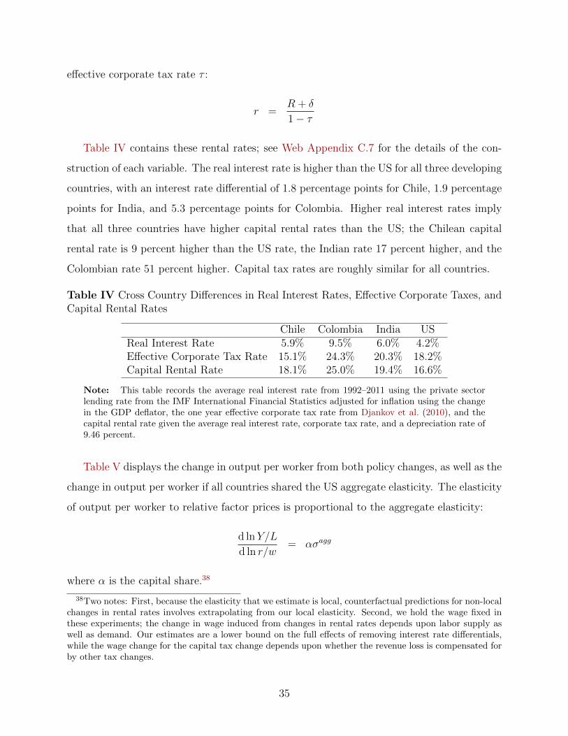
effective corporate tax rate τ :
r =R + δ
1− τ
Table IV contains these rental rates; see Web Appendix C.7 for the details of the con-
struction of each variable. The real interest rate is higher than the US for all three developing
countries, with an interest rate differential of 1.8 percentage points for Chile, 1.9 percentage
points for India, and 5.3 percentage points for Colombia. Higher real interest rates imply
that all three countries have higher capital rental rates than the US; the Chilean capital
rental rate is 9 percent higher than the US rate, the Indian rate 17 percent higher, and the
Colombian rate 51 percent higher. Capital tax rates are roughly similar for all countries.
Table IV Cross Country Differences in Real Interest Rates, Effective Corporate Taxes, andCapital Rental Rates
Chile Colombia India USReal Interest Rate 5.9% 9.5% 6.0% 4.2%Effective Corporate Tax Rate 15.1% 24.3% 20.3% 18.2%Capital Rental Rate 18.1% 25.0% 19.4% 16.6%
Note: This table records the average real interest rate from 1992–2011 using the private sectorlending rate from the IMF International Financial Statistics adjusted for inflation using the changein the GDP deflator, the one year effective corporate tax rate from Djankov et al. (2010), and thecapital rental rate given the average real interest rate, corporate tax rate, and a depreciation rate of9.46 percent.
Table V displays the change in output per worker from both policy changes, as well as the
change in output per worker if all countries shared the US aggregate elasticity. The elasticity
of output per worker to relative factor prices is proportional to the aggregate elasticity:
d lnY/L
d ln r/w= ασagg
where α is the capital share.38
38Two notes: First, because the elasticity that we estimate is local, counterfactual predictions for non-localchanges in rental rates involves extrapolating from our local elasticity. Second, we hold the wage fixed inthese experiments; the change in wage induced from changes in rental rates depends upon labor supply aswell as demand. Our estimates are a lower bound on the full effects of removing interest rate differentials,while the wage change for the capital tax change depends upon whether the revenue loss is compensated forby other tax changes.
35
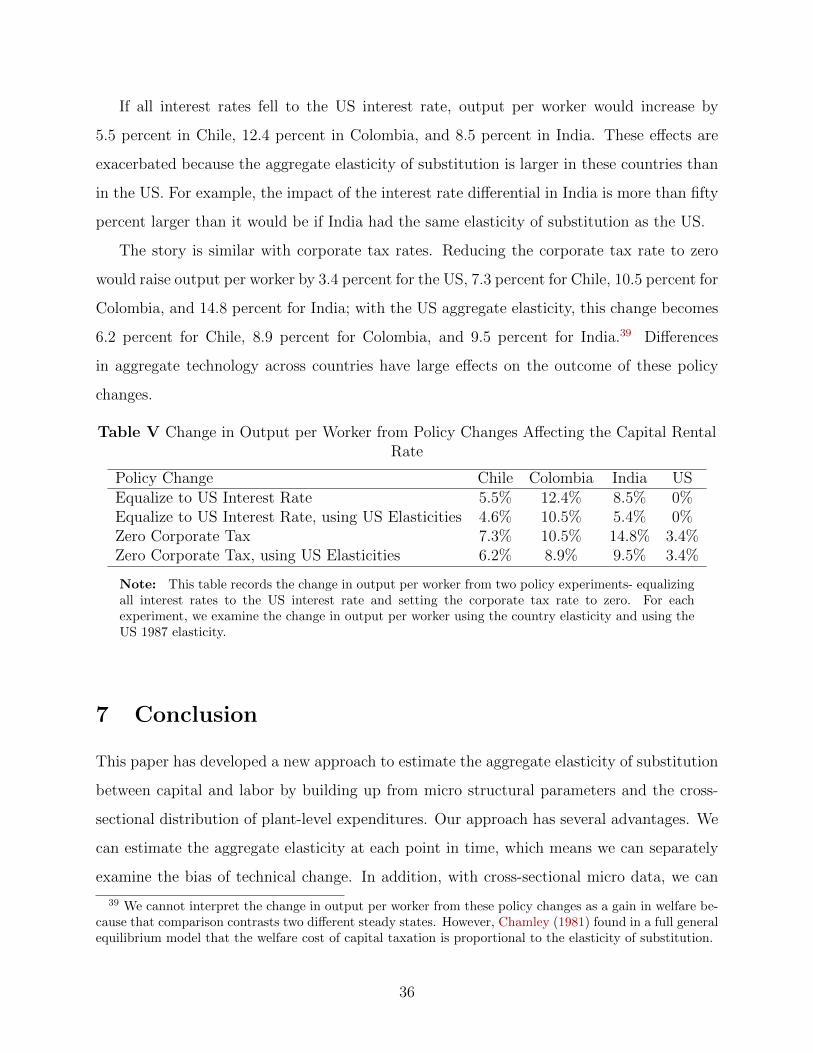
If all interest rates fell to the US interest rate, output per worker would increase by
5.5 percent in Chile, 12.4 percent in Colombia, and 8.5 percent in India. These effects are
exacerbated because the aggregate elasticity of substitution is larger in these countries than
in the US. For example, the impact of the interest rate differential in India is more than fifty
percent larger than it would be if India had the same elasticity of substitution as the US.
The story is similar with corporate tax rates. Reducing the corporate tax rate to zero
would raise output per worker by 3.4 percent for the US, 7.3 percent for Chile, 10.5 percent for
Colombia, and 14.8 percent for India; with the US aggregate elasticity, this change becomes
6.2 percent for Chile, 8.9 percent for Colombia, and 9.5 percent for India.39 Differences
in aggregate technology across countries have large effects on the outcome of these policy
changes.
Table V Change in Output per Worker from Policy Changes Affecting the Capital RentalRate
Policy Change Chile Colombia India USEqualize to US Interest Rate 5.5% 12.4% 8.5% 0%Equalize to US Interest Rate, using US Elasticities 4.6% 10.5% 5.4% 0%Zero Corporate Tax 7.3% 10.5% 14.8% 3.4%Zero Corporate Tax, using US Elasticities 6.2% 8.9% 9.5% 3.4%
Note: This table records the change in output per worker from two policy experiments- equalizingall interest rates to the US interest rate and setting the corporate tax rate to zero. For eachexperiment, we examine the change in output per worker using the country elasticity and using theUS 1987 elasticity.
7 Conclusion
This paper has developed a new approach to estimate the aggregate elasticity of substitution
between capital and labor by building up from micro structural parameters and the cross-
sectional distribution of plant-level expenditures. Our approach has several advantages. We
can estimate the aggregate elasticity at each point in time, which means we can separately
examine the bias of technical change. In addition, with cross-sectional micro data, we can
39 We cannot interpret the change in output per worker from these policy changes as a gain in welfare be-cause that comparison contrasts two different steady states. However, Chamley (1981) found in a full generalequilibrium model that the welfare cost of capital taxation is proportional to the elasticity of substitution.
36
examine the robustness of our model and identification strategy.
We then applied our methodology to data on plants in the US manufacturing sector.
While we estimated an average plant-level elasticity of roughly 0.5, our estimates indicated
that the aggregate elasticity of substitution between capital and labor has been close to
0.7 from 1972 to 2007. Thus roughly 63 percent of aggregate factor substitution happened
within plants.
We then measured the contributions of factor prices and two components of the bias of
technology to the fall of the labor share in manufacturing since 1970. To do this, we used our
estimates of aggregate elasticities and the history of factor prices. We found that the bias
of technical change within industries has steadily decreased the labor share, accounting for
most of the shift. There has been a sharp drop in the labor share since 2000 that coincides
with a shift in the composition of industries. We found that mechanisms that work through
factor prices alone cannot account for the decline in the labor share.
Our work indicates that explaining the decline in the labor share requires understanding
the determinants of technical change, broadly defined, including automation, IT investment,
offshoring, or shifts in composition driven by changing tastes or trade. Our decomposition
suggests that there may be more than one force at work. While we have applied our method-
ology to the change in the US labor share, we believe it can be useful in understanding the
evolution of skill premia and inequality.
Finally, our approach allowed us to estimate how the aggregate elasticity varies across
time and countries, and to understand the underlying reasons for such variation. In par-
ticular, greater heterogeneity in capital intensities implies a higher aggregate elasticity of
substitution. Elasticities in all three of the developing countries we examined were higher
than the US, with an average manufacturing sector elasticity of 0.84 for Chile, 0.84 for
Colombia, and 1.11 for India. Our estimates can help illuminate how and why policies have
differential effects across countries.
37
References
Acemoglu, Daron, “Directed Technical Change,” Review of Economic Studies, 2002, 69(4), 781–809.
, “Labor- And Capital-Augmenting Technical Change,” Journal of the European EconomicAssociation, 2003, 1 (1), 1–37.
, “When Does Labor Scarcity Encourage Innovation?,” Journal of Political Economy, 2010,118 (6), 1037–1078.
and Fabrizio Zilibotti, “Productivity Differences,” Quarterly Journal of Economics,2001, 116 (2), 563–606.
Alvarez-Cuadrado, Francisco, Ngo Van Long, and Markus Poschke, “Capital-LaborSubstitution, Structural Change and the Labor Income Share,” Technical Report, CESifoWorking Paper 2014.
Antras, Pol, “Is the US Aggregate Production Function Cobb-Douglas? New Estimates ofthe Elasticity of Substitution,” Contributions to Macroeconomics, 2004, 4 (1).
Atalay, Enghin, “How Important Are Sectoral Shocks?,” 2014. Mimeo.
Autor, David H., David Dorn, and Gordon H. Hanson, “The China Syndrome: LocalLabor Market Effects of Import Competition in the United States,” American EconomicReview, 2013, 103, 2121–68.
, Frank Levy, and Richard J. Murmane, “The Skill Content of Recent TechnologicalChange: An Empirical Exploration,” Quarterly Journal of Economics, 2003, 118, 1279–1333.
Banerjee, Abhijit and Esther Duflo, “Growth Theory Through The Lens Of Develop-ment Economics,” Handbook of Economic Growth, 2005, 1, 473–552.
Barnes, Sebastian N, Simon Price, and Maria Barriel, “The Elasticity of Substitu-tion: Evidence from a UK Firm-level Data Set,” 2008.
Bartik, Timothy J., Who Benefits from State and Local Economic Development Policies?,W. E. Upjohn Institute for Employment Research, 1991.
Bartlesman, Eric, John Haltiwanger, and Stefano Scarpetta, “Cross-Country Dif-ferences in Productivity: The Role of Allocation and Selection,” Technical Report 1 2013.
Berndt, Ernst R., “Reconciling Alternative Estimates of the Elasticity of Substitution,”Review of Economics and Statistics, 1976, 58 (1), 59–68.
Burstein, Ariel, Eduardo Morales, and Jonathan Vogel, “Accounting for Changes inBetween-Group Inequality,” 2014. Mimeo.
38
Caballero, Ricardo, Eduardo Engel, and John Haltiwanger, “Plant Level Adjust-ment and Aggregate Investment Dynamics,” Brookings Papers on Economic Activity, 1995,2, 1–54.
Chamley, Christophe, “The Welfare Cost of Capital Income Taxation in a Growing Econ-omy,” Journal of Political Economy, 1981, 89 (3), 468–96.
Chirinko, Robert S., “Sigma: The Long and Short of It,” Journal of Macroeconomics,2008, 30, 671–686.
, Steven M. Fazzari, and Andrew P. Meyer, “A New Approach to Estimating Pro-duction Function Parameters: The Elusive Capital-Labor Substitution Elasticity,” Journalof Business and Economic Statistics, 2011, 29 (4), 587–594.
Cummins, Jason and Giovanni Violante, “Investment-Specific Technical Change in theUS (1947-2000): Measurement and Macroeconomic Consequences,” Review of EconomicDynamics, 2002, 5 (2), 243–284.
Diamond, Peter, Daniel McFadden, and Miguel Rodriguez, “Measurement of theElasticity of Factor Substitution and Bias of Technical Change,” in Melvyn Fuss and DanielMcFadden, eds., Production Economics: A Dual Approach to Theory and Applications,1978, chapter 5.
Djankov, Simeon, Tim Ganser, Caralee McLiesh, Rita Ramalho, and AndreiSchliefer, “The Effect of Corporate Taxes on Investment and Entrepreneurship,” Amer-ican Economic Journal: Macroeconomics, 2010, 2 (3), 31–64.
Dornbusch, Rudiger, Stanley Fischer, and Paul Samuelson, “Heckscher-Ohlin TradeTheory with a Continuum of Goods,” Quarterly Journal of Economics, 1980, 95 (2), 203–224.
Elsby, Michael W. L., Bart Hobijn, and Aysegul Sahin, “The Decline of the U.S.Labor Share,” Brookings Papers on Economic Activity, 2013.
Fernald, John, “A Quarterly, Utilization-Adjusted Series on Total Factor Productivity,”September 2012. Mimeo.
Foster, Lucia, John Haltiwanger, and Chad Syverson, “Reallocation, Firm Turnover,and Efficiency: Selection on Productivity or Profitability?,” American Economic Review,March 2008, 98 (1), 394–425.
Gomme, Paul and Peter Rupert, “Measuring Labor’s Share of Income,” 2004. PolicyDiscussion Paper - No 7, Federal Reserve Bank of Cleveland.
Gordon, Robert J., The Measurement of Durable Goods Prices, University of ChicagoPress, 1990.
Greenstreet, David, “Exploiting Sequential Learning to Estimate Establishment-LevelProductivity Dynamics and Decision Rules,” 2007. Mimeo.
39
Hall, Robert E. and Dale W. Jorgenson, “Tax Policy and Investment Behavior,” Amer-ican Economic Review, 1967, 57 (3), 391–414.
Harper, Michael J., Ernst R. Berndt, and David O. Wood, “Rates of Return andCapital Aggregation Using Alternative Rental Prices,” in D.W. Jorgenson and R. London,eds., Technology and Capital Formation, Cambridge, MA: MIT Press, 1989.
Herrendorf, Berthold, Christopher Herrington, and Akos Valentinyi, “SectoralTechnology and Structural Transformation,” Technical Report 2014.
Hicks, John R., The Theory of Wages, MacMillan and Co, 1932.
Houthakker, Hendrik, “The Pareto Distribution and the Cobb-Douglas Production Func-tion in Activity Analysis,” The Review of Economic Studies, 1955, 23 (1), pp. 27–31.
Hsieh, Chang-Tai and Peter Klenow, “Misallocation and Manufacturing TFP in Chinaand India,” Quarterly Journal of Economics, 2009, 124 (4), 1403–1448.
Imbs, Jean and Isabelle Mejean, “Elasticity Optimism,” May 2011. Mimeo.
Jones, Chad, “The Shape of Production Functions and the Direction of Technical Change,”Quarterly Journal of Economics, 2005, 120 (2), 517–549.
Jorgenson, Dale W., Mun S. Ho, and John D. Samuels, “A Prototype Industry-levelProduction Account for the United States, 1947-2010,” 2013. Mimeo.
, , and Kevin J. Stiroh, “Growth of U.S. Industries and Investments in InformationTechnology and Higher Education,” in “Measuring Capital in the New Economy” NBERChapters, National Bureau of Economic Research, Inc, October 2005, pp. 403–478.
Karabarbounis, Loukas and Brent Neiman, “The Global Decline of the Labor Share,”Quarterly Journal of Economics, 2014, 129, 61–103.
Klump, Rainer, Peter McAdam, and Alpo Willman, “Factor Substitution and FactorAugmenting Technical Progress in the US,” Review of Economics and Statistics, 2007, 89(1), 183–192.
Krueger, Alan B., “Measuring Labor’s Share,” American Economic Review, 1999, 89 (2),45–51.
Krusell, Per, Lee Ohanian, Jose-Victor Rios-Rull, and Giovanni Violante,“Capital-skill Complementarity and Inequality: A Macroeconomic Analysis,” Economet-rica, 2000, 68 (5), 10291053.
Lagos, Ricardo, “A Model of TFP,” Review of Economic Studies, October 2006, 73 (4),983–1007.
Leon-Ledesma, Miguel A., Peter McAdam, and Alpo Willman, “Identifying theElasticity of Substitution with Biased Technical Change,” The American Economic Re-view, 2010, 100 (4), 1330–1357.
40
Levhari, David, “A Note on Houthakker’s Aggregate Production Function in a MultifirmIndustry,” Econometrica, 1968, 36 (1), pp. 151–154.
Luttmer, Erzo G. J., “Growth with a Fixed Factor,” 2012. Mimeo.
Mankiw, N. Gregory, “The Growth of Nations,” Brookings Papers on Economic Activity,1995, 1995 (1), 275–326.
Miyagiwa, Kaz and Chris Papageorgiou, “Endogenous Aggregate Easticity of Substi-tution,” Journal of Economic Dynamics and Control, 2007, 31 (9), 2899–2919.
Piketty, Thomas, Capital in the Twenty-First Century, Belknap Press, 2014.
Raval, Devesh, “The Micro Elasticity of Substitution and Non Neutral Technology,” 2014.Mimeo.
Restuccia, Diego and Richard Rogerson, “Policy Distortions and Aggregate Produc-tivity with Heterogeneous Establishments,” Review of Economic Dynamics, 2008, 11 (4),707–720.
Sato, Kazuo, Production Functions and Aggregation, Elsevier, 1975.
Tybout, James R. and Mark Roberts, Industrial Evolution in Developing Countries:Industrial Evolution in Developing Countries: Micro Patterns of Turnover, Productivityand Market Structure, Oxford University Press, 1996.
White, T Kirk, Jerome P Reiter, and Amil Petrin, “Plant-level Productivity and Im-putation of Missing Data in US Census Manufacturing Data,” Technical Report, NationalBureau of Economic Research 2012.
41
Appendix
A Proofs of Propositions
Appendix A describes the aggregate elasticity of substitution between capital and labor when eachplant’s production function exhibits constant returns to scale. Web Appendix B derives expressionsfor the aggregate elasticity under alternative assumptions. Web Appendix B.1 characterizes localelasticities of substitution and Web Appendix B.2 derives preliminary results under the assumptionthat plants’ production functions are homothetic. The assumption of constant returns to scaleis relaxed in Web Appendix B.3. Web Appendix B.4 introduces misallocation frictions. WebAppendix B.5 generalizes the demand system to allow for arbitrary elasticities of demand andimperfect pass-through. Web Appendix B.6 relaxes the assumption that production functions arehomothetic.
Throughout, we use the following notation for relative factor prices:
ω ≡ w
r
q ≡ q
r
In addition, we define pni ≡ Pni/r and pn ≡ Pn/r to be plant i’s and industry n’s prices respectivelynormalized by the rental rate. It will also be useful to define plant i’s cost function (normalized byr) to be
zni(Yni, ω, q) = minKni,Lni,Mni
Kni + ωLni + qMni subject to Fni(Kni, Lni,Mni) ≥ Yni
and industry n’s cost as zn =∑
i∈In zni. Two results will be used repeatedly. First, Shephard’slemma implies that for each i:
(1− sMni )(1− αni) =∂ ln zni∂ lnω
(14)
sMni =∂ ln zni∂ ln q
(15)
Second, since αn =∑
i∈In αniθni, then for any quantity κn,∑i∈In
(αni − αn)κnθni = 0 (16)
When production functions take the functional form in defined in Assumption 1, it is relativelystraightforward to derive the industry-level elasticity of substitution. However, when we aggregateacross industries, we have no justification for using any particular functional form for the industry-level production function, or how capital, labor, and materials are nested in the industry-levelproduction function. We will therefore derive a formula for the industry-level elasticity of substi-tution in a way that nests nicely: the same formula used to go from plant-level to industry-levelcan be used to go from industry level to aggregate.
Consequently here we relax the functional form assumption on plants’ production functions.While we maintain that each plant’s production function has constant returns to scale, we impose
42
no further structure.
Assumption 1′ Plant i in industry n uses the constant returns to scale production functionFni(Kni, Lni,Mni).
The purpose of this is twofold. First, it provides guidance on the robustness of the formulas inProposition 1. Second, we will later use the formulas here to aggregate across industries and derivean expression for the elasticity of substitution between capital and labor for the manufacturingsector as a whole.
For plant i, we define the local elasticities σni and ζni to satisfy
σni − 1 =d lnKni/ωLni
d lnω(17)
ζni − 1 =1
αM − αnid ln qMni
Kni+ωLni
d lnω(18)
If i’s production function takes a nested CES form as in Assumption 1, σni and ζni would equalσn and ζn respectively.40 Under Assumption 1′, they are defined locally in terms of derivatives ofFni evaluated at i’s cost-minimizing input bundle. Exact expressions for σni and ζni are given inWeb Appendix B.1 of the web appendix. Proposition 1′ then expresses the industry elasticity ofsubstitution σNn . The resulting expression is identical to Proposition 1 except the plant elasticitiesof substitution are replaced with weighted averages of the plants’ local elasticities, σ̄n and ζ̄n.
Proposition 1′ Under Assumption 1′, the industry elasticity of substitution σNn = d lnKn/Lnd lnω is:
σNn = (1− χn)σ̄n + χn[(1− s̄Mn )εn + s̄Mn ζ̄n
](19)
where χn ≡∑
i∈In(αni−αn)2θniαn(1−αn) and s̄Mn ≡
∑i∈In
(αni−αn)(αni−αM )∑j∈In (αnj−αn)(αnj−α
M )sMni as in Proposition 1 and
σ̄n ≡∑i∈In
αni(1− αni)θni∑j∈In αnj(1− αnj)θnj
σni
ζ̄n ≡∑i∈In
(αni − αn)(αni − αM )sMni∑j∈In(αnj − αn)(αnj − αM )sMnj
ζni
Proof. As discussed in the text, the definitions of σni and σNn imply
σni − 1 =d ln rKni
wLni
d lnω=
1
αni(1− αni)dαnid lnω
, ∀i ∈ In
σNn − 1 =d ln rKn
wLn
d lnω=
1
αn(1− αn)
dαnd lnω
40The definition of σni is straightforward but ζni requires some elaboration. Suppose that Fni takes the
nested CES form of Assumption 1. Let λni ≡ 1r
[(r/Ani)
1−σn + (w/Bni)1−σn
] 1σn−1 be the marginal cost of
i’s capital-labor bundle. Then cost minimization implies qMni
Kni+ωLni=(
q/Cniλni
)1−ζn. Since d ln q
d lnω = 1 − αM
and, from Shephard’s Lemma, d lnλnid lnω = 1− αni, we have thatd ln
qMniKni+ωLni
d lnω = (ζn − 1)(αM − αni).
43
Since αn =∑
i∈In αniθni, we can differentiate to get
σNn − 1 =1
αn(1− αn)
[∑i∈In
dαnid lnω
θni +∑i∈In
αnidθnid lnω
]
=
∑i∈In αni(1− αni)θni(σni − 1)
αn(1− αn)+
∑i∈In αni
dθnid lnω
αn(1− αn)
Using the definition of σ̄n and∑
i∈Indθnid lnω = 0, we have
σNn − 1 = (σ̄n − 1)∑i∈In
αni(1− αni)θniαn(1− αn)
+
∑i∈In(αni − αn) dθnid lnω
αn(1− αn)(20)
Since χn =∑
i∈In(αni−αn)2θniαn(1−αn) , one can verify that
∑i∈In
αni(1−αni)θniαn(1−αn) = 1− χn, which gives
σNn = (1− χn)σ̄n +
∑i∈In(αni − αn) dθnid lnω
αn(1− αn)+ χn (21)
We now find an expression for d ln θnid lnω . θni can be written as
θni =rKni + wLni∑
j∈In rKnj + wLnj=
(1− sMni )zni∑j∈In(1− sMnj)znj
=(1− sMni )zni(1− sMn )zn
Since d ln1−sMnisMni
= 1sMnid ln(1− sMni ), the definition of ζn implies
d ln(1− sMni )d lnω
= sMni (ζn − 1)(αni − αM )
The change in i’s expenditure on all inputs depends on its expenditure shares:
znizn
=rKni + wLni + qMni∑
j∈In rKnj + wLnj + qMnj=
εn−1εn
PniYni∑j∈In
εn−1εn
PnjYnj=
εn−1εn
P 1−εnni YnP
εnn∑
j∈Inεn−1εn
P 1−εnnj YnP
εnn
=
(pnipn
)1−εn
The change in i’s price depends on the change in its marginal cost
d ln pnid lnω
=d ln εn
εn−1mcni
d lnω=d lnmcnid lnω
= (1− sMni )(1− αni) + sMni (1− αM ) (22)
Putting these pieces together, we have θni =1−sMni1−sMn
(pnipn
)1−εn, so differentiating and using equa-
44
tion (16) yields
∑i∈In
(αni − αn)θnid ln θnid lnω
=∑i∈In
(αni − αn)θni
[d ln 1− sMnid lnω
+ (1− εn)d ln pnid lnω
]
=∑i∈In
(αni − αn)θni
{sMni (ζni − 1)(αni − αM )
+(1− εn)[(1− sMni )(1− αni) + sMni (1− αM )
] }=
∑i∈In
(αni − αn)θni{sMni (ζni − εn)(αni − αM ) + (1− εn)(1− αni)
}Using the definitions of ζ̄n, s̄Mn , and χn, this becomes∑i∈In
(αni − αn)θnid ln θnid lnω
=∑i∈In
(αni − αn)θni[sMni (ζ̄n − εn)(αni − αM ) + (1− εn)(1− αni)
]=
∑i∈In
(αni − αn)θni[s̄Mn (ζ̄n − εn)(αni − αM ) + (1− εn)(1− αni)
]=
∑i∈In
(αni − αn)θni[s̄Mn (ζ̄n − εn)(αni − αn) + (1− εn)(αn − αni)
]= αn(1− αn)χn
[(ζ̄n − εn)s̄Mn − (1− εn)
]Finally, we can plug this back into equation (21) to get
σNn = (1− χn)σ̄n + χn[s̄Mn ζn + (1− s̄Mn )εn
]To build up to the aggregate elasticity of substitution between capital and labor, we proceed in
exactly the same way as with the industry-level elasticity. Define ζNn to satisfy (ζNn −1)(αn−αM ) =
d ln1−sMnsMn
d lnω . The claim below will give an expression for ζNn in terms of plant level elasticities andchoices.
Proposition 2′ Under Assumption 1′, the aggregate elasticity between capital and labor is
σagg = (1− χN )σ̄N + χN[s̄M ζ̄N + (1− s̄M )η
]
45
where χN , σ̄N , ζ̄N , s̄M , and ζNn are defined as
χN =∑n∈N
(αn − α)2θnα(1− α)
σ̄N =∑n∈N
αn(1− αn)θn∑n′∈N αn′(1− αn′)θn′
σNn
ζ̄N ≡∑
n∈N (αn − α)(αn − αM )θnsMn ζ
Nn∑
n∈N (αn − α)(αn − αM )θnsMn
s̄M =
∑n∈N (αn − α)(αn − αM )θns
Mn∑
n∈N (αn − α)(αn − αM )θn
ζNn =∑i∈In
θni
[ζni
sMni (αni − αM )
sMn (αn − αM )+ εn
{1− sMni (αni − αM )
sMn (αn − αM )
}]
Proof. Note that since znizn
= PniYniPnYn
, we have both d lnYnd lnω =
∑i∈In
znizn
d lnYnid lnω and d ln pn
d lnω =∑i∈In
znizn
d ln pnid lnω . With the first, we can derive an expression for the change in cost that paral-
lels equation (27):
d ln znd lnω
=∑i∈In
znizn
d ln znid lnω
=∑i∈In
znizn
[d lnYnid lnω
+ (1− sMni )(1− αni) + sMni (1− αM )
]=
d lnYnd lnω
+ (1− sMn )(1− αn) + sMn (1− αM )
With the second, we can derive an expression for the change in the price level that parallelsequation (22)
d ln pnd lnω
=∑i∈In
znizn
d ln pnid lnω
=∑i∈In
(1− αni)(1− sMni ) + sMni (1− αM )
= (1− αn)(1− sMn ) + sMn (1− αM )
Thus following the exact logic of Proposition 1′, we have that
σagg = (1− χN )σ̄N + χN[s̄M ζ̄N + (1− s̄M )η
]It remains only to derive the expression for ζNn . Begin with 1− sMn =
∑i∈In(1− sMni )
znizn
. Differen-tiating each side gives:
d ln(1− sMn )
d lnω=∑i∈In
(1− sMni )zni(1− sMn )zn
[d ln(1− sMni )
d lnω+d ln zni/znd lnω
]=∑i∈In
θni
[d ln(1− sMni )
d lnω+d ln zni/znd lnω
]
46
Using (αni − αM )(ζni − 1) = 1sMni
d ln(1−sMni)d lnω and (αn − αM )(ζNn − 1) = 1
sn
d ln(1−sMn )d lnω gives
sMn (αn − αM )(ζNn − 1) =∑i∈In
θni
[sMni (αni − αM )(ζni − 1) +
d ln zni/znd lnω
]Finally, we have
d ln zni/znd lnω
=d lnYnid lnω
+ (1− sMni )(1− αni) + sMni (1− αM )− d lnYnd lnω
− (1− sMn )(1− αn)− sMn (1− αM )
= (−εn)d ln pni/pnd lnω
+ (1− sMni )(1− αni) + sMni (1− αM )− (1− sMn )(1− αn)− sMn (1− αM )
= (1− εn)[(1− sMni )(1− αni) + sMni (1− αM )− (1− sMn )(1− αn)− sMn (1− αM )
]= (εn − 1)
[sMn (αn − αM )− sMni (αni − αM ) + (αni − αn)
]Plugging this in, we have
sMn (αn − αM )(ζNn − 1) =∑i∈In
θni
{sMni (αni − αM )(ζni − 1)
+(εn − 1)[sMn (αn − αM )− sMni (αni − αM ) + (αni − αn)
] }
Using∑
i∈In θni(1− εn)(αni − αn) = 0, dividing through by sMn (αn − αM ) and subtracting 1 fromeach side gives the result.
47