metrologia measurementoftheplanckconstantatthenational ... · metrologia...

arX

iv:1

708.

0247

3v1

[ph

ysic

s.in

s-de

t] 8

Aug

201

7metrologia

Measurement of the Planck constant at the NationalInstitute of Standards and Technology from 2015 to 2017

D. Haddad1, F. Seifert1,2,L.S. Chao1, A. Possolo1,D.B. Newell1, J.R. Pratt1,C.J. Williams1,2,S. Schlamminger1

Abstract.Researchers at the National Institute of Standards and Technology(NIST) have measured the value of thePlanck constant to be h = 6.626 069 934(89)× 10−34 J s (relative standard uncertainty 13× 10−9). The resultis based on over 10 000 weighings of masses with nominal values ranging from 0.5 kg to 2 kg with the Kibblebalance NIST-4. The uncertainty has been reduced by more than twofold relative to a previous determinationbecause of three factors: (1) a much larger data set than previously available, allowing a more realistic,and smaller, Type A evaluation; (2) a more comprehensive measurement of the back action of the weighingcurrent on the magnet by weighing masses up to 2 kg, decreasing the uncertainty associated with magnet non-linearity; (3) a rigorous investigation of the dependence of the geometric factor on the coil velocity reducingthe uncertainty assigned to time-dependent leakage of current in the coil.

1. Introduction

This article summarizes measurements that were car-ried out with the Kibble balance, NIST-4, at the Na-tional Institute of Standards and Technology (NIST)from December 22, 2015 to April 30, 2017. A de-tailed description of NIST-4 and a first determinationof the Planck constant h with a relative standard un-certainty of 34 × 10−9 can be found in [1]. Sincethe previous result, several improvements to NIST-4 have been made. More importantly, many carefulmeasurements and systematic investigations have im-proved our understanding of the apparatus, leading tosmaller estimates of three dominating uncertainties.

2. The theory of the Kibble balance

The principle of the Kibble balance, formerly knownas watt balance, was first published by Bryan Kib-ble, [2] a metrologist at the National Physical Labo-

.D. Haddad1, F. Seifert1,2, L.S. Chao1, A. Possolo1,D.B. Newell1, J.R. Pratt1, C.J. Williams1,2,S. Schlamminger1: 1National Institute of Standardsand Technology (NIST), 100 Bureau Drive Stop 8171,Gaithersburg, MD 20899, USA2University of Maryland, Joint Quantum Institute, CollegePark, MD 20742, USA

ratory in the United Kingdom. This section intro-duces the theory necessary to understand the im-provements that led to the new result presentedhere, but it does not contain the complete theoryof the Kibble balance. A comprehensive discussionof the principle of the Kibble balance can be foundin [3, 4]. The Kibble balance has a long history atNIST [5, 6, 7, 8, 9, 10, 11, 12] and the designationNIST-4 indicates that this is the fourth instrumentthat has been built and operated by researchers atNIST. Throughout the world several Kibble balancesare being constructed or operated [13, 14, 15, 16, 17].

Common to NIST-1 through NIST-4 is that awheel is used for both the balancing and movingmechanisms. The wheel pivots about a knife edgecollinear with the wheel’s central axis. A measure-ment coil and test mass are suspended from one sideof the wheel while a tare mass is suspended from theother via multi-filament bands. The tare mass in-cludes a small motor consisting of a coil in a per-manent magnet system, similar in design but muchsmaller than the main magnet, for generating a forceto rotate the wheel. The benefit of a wheel versus atraditional balance beam is that the former prescribesa pure vertical motion for the suspended coil whereasthe latter traces an arc.

The measurement is performed in two modes:force and velocity mode. In force mode, a currentI in a coil with a wire length l immersed in a ra-

Metrologia, 2016, 00, 1-11 1

http://arxiv.org/abs/1708.02473v1

D. Haddad1, F. Seifert1,2, L.S. Chao1, A. Possolo1, D.B. Newell1, J.R. Pratt1, C.J. Williams1,2, S. Schlamminger1

dial magnetic field with magnetic flux density B iscontrolled such that the balance wheel remains at aconstant angle chosen by the operator. While the bal-ance wheel is servo controlled, a mass standard witha mass m, typically 1 kg, can be placed on or removedfrom the mass pan. Without the mass standard onthe pan, the electromagnetic force balances the excessmass on the tare side mt (usually about m/2):

IOff(Bl)F = mtg. (1)

Here, g denotes the local acceleration of gravity and(Bl)F is the geometric factor of the magnet and coilcombination, the product of B and l as measured inforce mode. The current in the coil for the mass-offstate is denoted by IOff . With the mass standard onthe mass pan, the current reverses to IOn and theforce equation is

IOn(Bl)F −mg = mtg. (2)

Subtracting equation 2 from 1 and solving for (Bl)Fyields

(Bl)F =mg

IOn − IOff

. (3)

Generally, the best results can be achieved bysymmetrizing the measurement and the instrumentas much as possible. Specifically, this is achieved byadjusting mt = m/2, which results in the two equalbut opposite currents. The advantage of using sym-metric currents is explained in detail in section 4.2..

The geometric factor is also obtained in velocitymode, where the coil is swept through the magneticfield by rotating the wheel with the tare-side motor.During the coil sweep, the induced voltage U and thecoil’s velocity v are measured simultaneously. Thesecoil sweeps can move either downward, with negativevelocity (vdn < 0) or upward, with positive velocity(vup > 0). The geometric factor in the velocity modeis determined by

(Bl)V =1

2

(

Uup

vup+

Udn

vdn

)

. (4)

The up and down measurements are necessary to can-cel small thermal and other parasitic voltages presentin the circuit. These voltages are approximately a fewhundred nanovolts. By averaging the measured geo-metric factors for up and down sweeps, these extravoltages cancel, as long as they remain constant overthe duration of the sweeps and vup = −vdn.

The ratio of the two measurements of the geomet-ric factor (Bl)F and (Bl)V is nominally one. The me-chanical quantities are measured in the InternationalSystem of Units (SI), whereas the electrical quanti-ties are measured in conventional units, denoted by

the subscript 90, hence

(Bl)F(Bl)V

=(Bl)F N

A90

(Bl)VV90 s

m

Nms−1

V90 A90

=(Bl)F N

A90

(Bl)VV90 s

m

W

W90

.

(5)The terms in the numerator and denominator of theratio are written as products of numerical quantitiesand units. The numerical quantity is indicated by thecurly brackets in the units given by the subscript.The last term of Equation 5 is a ratio of watts ex-pressed in the International System of Units (SI) andconventional units. The ratio must be equal to one,since both measurements are determining the samephysical quantity, the geometric factor. Hence,

(Bl)F N

A90

(Bl)VV90 s

m

=W90

W. (6)

The value one can be written as the Planck con-stant divided by the Planck constant. Expanding thenumerator as the product of a numerical quantity andthe SI-unit and the denominator as a numerical quan-tity and the conventional unit yields

1 =hWs2

hW90 s2

Ws2

W90 s2

and thushWs2

hW90 s2=

W90

W.

(7)By combining equations 6 and 7, an equation for thenumerical value of the Planck constant can be ob-tained,

hSIh90

=(Bl)F(Bl)V

. (8)

In equation 8, the expressions hSI and h90 arethe numerical values of the Planck constant in SI andin conventional units, respectively. To define the con-ventional units, the numerical values of the conven-tional Josephson constant and the conventional vonKlitzing constant were fixed in 1990 [18]. From thesenumerical values, the numerical value of the Planckconstant in the conventional unit system can be ob-tained,

h90 = 6.626 068 854 361 . . .× 10−34. (9)

3. Overview of the data

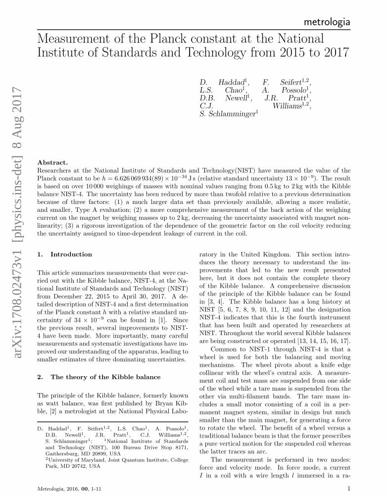
The measurements are organized in runs typicallylasting about a day each. A run usually comprises tensets of determinations of the geometric factors. Fig-ure 1 shows the measured geometric factors in forceand velocity modes for a typical run. A set consistsof three groups of measurements, two velocity groupsand one force group. In each velocity group the coilis swept 30 times through the magnetic field in alter-nating directions (down, up, down, etc.). Each force

2 Metrologia, 2016, 00, 1-11

Measurement of the Planck constant at the National Institute of Standards and Technology from 2015 to 2017

group contains 17 weighings, alternating nine withthe mass on the balance pan and eight with the massoff the balance pan.

709.4300

709.4302

Bl

2 × 10−7

BlV

BlF

−1000

100

0 5 10 15 20 25

time (h)

−1000

100

fit−

Bl

Bl

×10

9

Figure 1. A data run started on November 15 2016. Thedata is typical for NIST-4. Groups of measurements invelocity and force mode are carried out in an alternatingpattern. The scatter in a velocity group is several timesthe scatter of the data in force mode. The blue and blackline segments are second order polynomials that are fit-ted to three groups of data (velocity, force, velocity). Theinner velocity groups are part of two fits (one shown inblack, the other in blue). Their respective relative resid-uals are shown in the two plots below the main panel.

Figure 1 shows the data collected in a typical runthat was started at 15:21 local time on November 15,2016. The run was terminated at 16:10 the next dayby the operator and yielded ten data sets. One mea-surement of the Planck constant is derived from thedata in each set. The measured value is obtainedfrom the difference in the zeroth order term of a sec-ond degree polynomial fitted separately to the dataobtained in velocity mode and in force mode. Theblue and black segments in Figure 1 show the poly-nomial fits to every other set. Each velocity group,other than the very first and very last group is usedfor two adjacent h measurements. The residuals ofthe polynomial fits are shown in the lower two graphsof Figure 1.

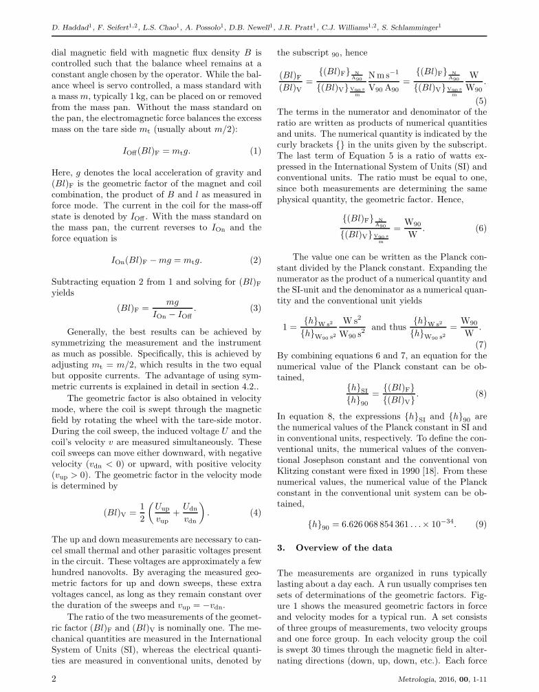
For the data discussed in this paper, a totalof 1174 sets were measured from December 2015through April 2017. Figure 2 shows the h measure-ments for all sets. A total of eight different combina-tions of masses were used. To combine the mass val-ues we used a total of five stainless steel (SS) masseswith a nominal value of 0.5 kg, one stainless steelmass with a nominal value of 1 kg, and two Platinum-Iridium prototypes, labelled K85 and K104. Figure 3shows the average value of h for each mass combina-tion used in the experiment. The top diagram in the

12/

15

02/

16

04/

16

06/

16

08/

16

10/

16

12/

16

02/

17

04/

17

time (month/year)

50

100

150

200

250

h S

I−h

90

h 9

0×

109

improvedinterferometers

blockfloats

SS, 12 kg

K85, 1 kg

K104, 1 kg

SS, 2 × 12 kg

SS, 1 kg

K85+SS, 12 kg

SS, 3 × 12 kg

K85+K104, 2 kg

0 100counts

Figure 2. The complete data set used for this determi-nation of the Planck constant. Data taken with stainlesssteel masses are abbreviated as SS, the Platinum-Iridiumprototypes are designated as K85 and K104. The solidhorizontal line indicates the final measurement result andthe two dashed lines are drawn ±13×10−9 away from theresult.

figure shows the number of sets that were measuredfor each mass combination. The majority of the datawere obtained using K85 and K104 with 347 and 389sets, respectively.

0.5 1 1 1 1 1.5 1.5 2nominal mass / kg

140

150

160

170

180

h S

I−h

90

h 9

0×

109

SS K85 K104SSx 2 SS

K85SS

SSx 3

K85K104

0200400

sets

Figure 3. The lower graph shows values of h as a func-tion of mass. A total of eight masses or mass combi-nations were used. The lower horizontal axis shows thenominal value, while the upper horizontal axis indicatesthe stacking that was used to obtain these values. The ab-breviation SS stands for stainless steel and K85 and K104denote two Pt-Ir prototypes. The upper graph shows thenumber of sets that were obtained for each mass or masscombination.

The relative standard deviation of the velocityand force residuals shown in Figure 1 are 35 × 10−9

and 12 × 10−9. The residuals in velocity mode wereimproved during the summer 2016. The relative stan-

Metrologia, 2016, 00, 1-11 3


dard deviation of the residuals in one velocity groupranged from 30× 10−9 to 60× 10−9 before and from23 × 10−9 to 50 × 10−9 after summer 2016. A sec-ond improvement was achieved at the end of March2017 by installing a vibration isolation system. Eightair springs and a commercially available pneumaticcontroller position lift the concrete block supportingNIST-4 by 10mm off the building’s foundation whilemaintaining its pitch and roll angle to within fewµrad. Floating the block on air springs reduced thevibrational excitation of NIST-4 significantly. Withthe block floated, the relative standard deviation ofthe residuals in velocity mode are in the range from11 × 10−9 to 25 × 10−9. Interestingly, the residualsof the fits to each individual volt-velocity profile im-proved by an order of magnitude, while the standarddeviation of the residuals in velocity mode only de-creased by a factor two. We assume that, after float-ing the block, the standard deviation of the residualsis limited by the variability from one sweep to thenext.

The first reduction in the scatter of the residu-als, over the summer of 2016, was achieved by sub-stantially stiffening the base plates and optimizingthe mounting technique of the three interferometersused to measure the velocity of the coil. Beforethat time, each interferometer was screwed to thebase plate of the Kibble balance. Three mountingplates made from 25.4mm thick aluminium, each sup-porting one interferometer and turning mirrors, weremated to the base plate through kinematic mounts.This thicker plate and improved mounting to the Kib-ble balance decreased vibrational coupling, parasiticmotions, and internal contortions of the interferome-ters which led to the visible reduction of the scatterin Figure 2. No data were included from the end ofMay 2016 to the beginning of November 2016, eventhough some data were collected during this period.The work was focused on improving the statisticaluncertainty and not on collecting science data.

The measurements of (Bl)F contain a measuredvalue of the local acceleration of gravity g using anabsolute gravimeter. For the majority of the data pre-sented here, the absolute gravimeter was operated si-multaneously with the Kibble balance. Commerciallyavailable software was used to calculate the time de-pendent part of g and added to the last measuredvalue. The output of the software has been verified byusing long data sets (several months) obtained withthe absolute gravimeter in the Kibble balance labo-ratory. The effects included in the calculation of gare tidal effects of the sun and moon, ocean loading,effects due to atmospheric pressure, and the effect ofpolar motion. The value of g at the test mass centreis tied from the absolute reference in the laboratoryand corrected for the vertical gradient of g [19, 20].

The vertical gravity gradient was measured three dif-ferent times at the mass pan location. Other thanbeing corrected for g, the data shown in Figure 1 isobtained from raw voltmeter readings and the volt-age setting of the Programmable Josephson VoltageStandard. For the interferometer readings, the Abbeoffset is considered when combining the three inter-ferometers.

−10

0

10

vir

tual

po

wer

−10

0

10

ver

tica

lity

12/

15

02/

16

04/

16

06/

16

08/

16

10/

16

12/

16

02/

17

04/

17

time (month/year)

−10

0

10

fiel

dg

rad

ien

t

rel.

bia

s×

109

du

eto

SS, 12 kg

K85, 1 kg

K104, 1 kg

SS, 2 × 12 kg

SS, 1 kg

K85+SS, 12 kg

SS, 3 × 12 kg

K85+K104, 2 kg

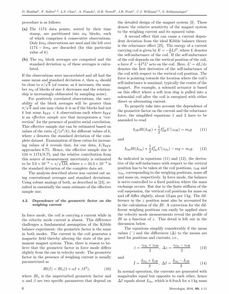
Figure 4. The alignment biases that have to be sub-tracted from the raw data of each set in order to obtainthe values shown in Fig. 2. The horizontal blue lines showthe averages of the biases. The three average values ofthe relative biases are between 0 and 1 × 10−9. Datataken with stainless steel masses are abbreviated as SS,the Platinum-Iridium prototypes are designated as K85and K104.

The raw measurements of the geometric factors invelocity and force mode contain a number of biasesthat need to be subtracted to obtain the final valuesof h. Every time a bias is subtracted from the data,an uncertainty is added to the result because the biasis not precisely known.

For NIST-4, three different categories of biasesneed to be considered: (1) the back action of the cur-rent in the coil during force mode on the magneticfield; (2) diffraction and wavefront distortion in themeasurement of the coil velocity with the three inter-ferometers; (3) the alignment of the balance, the coiland the interferometers. The biases caused by themagnetic fields are discussed in detail below. Com-prehensive information on the alignment biases canbe found in [1] and [21]. In brief, these alignmentbiases can be divided into three groups

4 Metrologia, 2016, 00, 1-11


Virtual power contains the sum of five relative par-asitic power terms. These are the products ofnon-vertical forces and torques on the coil inforce mode with non-vertical velocities and an-gular velocities in velocity mode. For examplethe term Fx vx/(Fz vz) is the parasitic power inthe x - direction. The other four terms are trans-lation in y and rotations around the x, y, and zaxes. A discussion of these terms is given in [21].

Verticality collects four terms that arise from slightmisalignment of the three interferometer beamswith respect to g. Three of the four terms arethe result of a parasitic motion of the coil in ve-locity mode. A translation along x, y, and arotation about z of the coil can attenuate or aug-ment the measured vertical velocity of the coil: aperfect vertical laser beam is insensitive to a dis-placement perpendicular to the direction of thelaser beam. But if the laser beam is slightly mis-aligned, then a parasitic horizontal displacementwill have a component along the direction of thelaser beam. The fourth term is independent ofthe coil’s parasitic motion and reflects the factthat if a measurement beam deviates from verti-cality by α, the measured velocity is attenuatedand will be cos (α) times the vertical velocity.

Field gradient consists of four terms that capturethe relative difference in the geometric factor be-tween velocity mode and force mode. The coilposition in force mode is not exactly on the tra-jectory of the coil in velocity mode and a cor-rection must be applied. Therefore, the differ-ences of the coil position in force mode to thecoil trajectory in x, y, θx, and θy are multipliedby the measured derivatives of the geometric fac-tors with respect to these directions.

Figure 4 shows the relative correction that needsto be subtracted from the raw data as a result of thethree types of alignment biases. The blue horizontallines in Figure 4 are the values obtained by averagingthe corrections over all data sets. The averages are0.2× 10−9, 0.2× 10−9, and 0.7× 10−9 for the biasescaused by virtual power, verticality, and field gradi-ents, respectively. The averages are very small andoverall the biases have a negligible effect (relativelyat most 1.1× 10−9) on the reported result.

Figure 4 also shows how often the alignment waschecked and the apparatus realigned. For example,it can be seen that the verticality of the interferome-ters was measured almost every time the mass in theexperiment was changed.

4. Improved understanding of the apparatus

The relative standard uncertainty of the result givenhere is less than half of that published previously [1].This improvement is due to smaller uncertainties inthree categories of the uncertainty budget (Table 1.1)labelled statistical, magnetic field, and electrical. Inthe following three sections, the new uncertainty es-timates for these three categories are discussed.

4.1. Estimation of the statistical uncertainty

In the 2016 publication, the relative statistical uncer-tainty was estimated to be 24.9×10−9, obtained fromthe standard deviation of the 125 determinations thatwere incorporated into the corresponding estimate ofh. This assigned uncertainty was very conservativebecause the uncertainty associated with an averageis generally smaller than the uncertainty associatedwith the observations that are averaged. If n obser-vations, each with the same uncertainty, are uncorre-lated, then their average will have an uncertainty thatis

√n smaller than their common, individual uncer-

tainty. However, since the 2016 estimate was basedon only 13 days of data, it was not quite possible todetect and characterize any pattern of correlations re-liably. Furthermore, given the level of familiarity withthe instrument at the time, it was difficult to ascertainwhether the series of measured values was stationary.Both the inability to gauge auto-correlations mean-ingfully and the lack of clarity regarding stationarityled us to adopt a rather conservative assessment ofthis component of uncertainty.

The current measurement of h is based on dataacquired over the course of about 16 months whichproduced 1174 individual determinations of h, de-picted in Figure 2. During this long period, the Kib-ble balance underwent several mechanical upgrades.The multi-filament band connecting the main coil tothe wheel was replaced by a similar band with highertensile strength. As stated earlier, the three inter-ferometers were remounted on thicker, kinematicallymounted base plates. Additional optics were installedor replaced in the interferometers to better measurethe laser beam verticality, reduce frequency leakage,and measure the parasitic coil motion. Eight differentmasses or combinations of masses were employed forthis measurement duration. Finally, the instrumentwas completely realigned on several occasions. Still,the resulting values of h remained essentially constantduring this period (Figure 2).

To determine whether the standard error of anaverage of n consecutive observations is inversely pro-portional to

√n, we undertook a sub-sampling anal-

ysis similar to [22]. Refer to [23] for a detailed de-scription of sub-sampling methods in general. The

Metrologia, 2016, 00, 1-11 5


procedure is as follows:

(a) The 1174 data points, sorted by their timestamp, are partitioned into mk blocks, eachof which comprises k consecutive observations.Only kmk observations are used and the left over1174 − kmk are discarded (for this particularvalue of k).

(b) The mk block averages are computed and thestandard deviation sk of these averages is calcu-lated.

If the observations were uncorrelated and all had thesame mean and standard deviation σ, then sk shouldbe close to σ/

√k (of course, as k increases, the num-

ber mk of blocks of size k decreases and the relation-ship is increasingly obfuscated by sampling noise).

For positively correlated observations, the vari-ability of the block averages will be greater thanσ/

√k and one may claim it is as if the blocks had not

k but some kEFF < k observations each where kEFF

is an effective sample size that incorporates a “cor-rection” for the presence of positive serial correlation.This effective sample size can be estimated based onvalues of the ratio s2k/(s

2/k), for different values of k,where s denotes the standard deviation of the com-plete dataset. Examination of these ratios for increas-ing values of k reveals that, for our data, k/kEFF

approaches 8.75. Hence, the effective sample size is134 ≈ 1174/8.75, and the relative contribution fromthis source of measurement uncertainty is estimatedto be 3.0× 10−9 = s/

√134, where s = 34.3× 10−9 is

the standard deviation of the complete data set.The analysis described above was carried out us-

ing conventional averages and standard deviations.Using robust analogs of both, as described in [24], re-sulted in essentially the same estimate of the effectivesample size.

4.2. Dependence of the geometric factor on theweighing current

In force mode, the coil is carrying a current while inthe velocity mode current is absent. This differencechallenges a fundamental assumption of the Kibblebalance experiment: the geometric factor is the samein both modes. The current in the coil generates amagnetic field thereby altering the state of the per-manent magnet system. Thus, there is reason to be-lieve that the geometric factor in force mode differsslightly from the one in velocity mode. The geometricfactor in the presence of weighing current is usuallyparametrized as

Bl(I) = Blo(1 + αI + βI2), (10)

where Blo is the unperturbed geometric factor andα and β are two specific parameters that depend on

the detailed design of the magnet system [3]. Thesedenote the relative sensitivity of the magnet systemto the weighing current and its squared value.

A second effect that can cause a current depen-dent deviation from the ideal Kibble balance theoryis the reluctance effect [25]. The energy of a currentcarrying coil is given by E = − 1

2LI2, where L denotes

the self-inductance of the coil. If the self-inductanceof the coil depends on the vertical position of the coil,a force F = 1

2I2L′ acts on the coil. Here, L′ = dL/dz

denotes the first derivative of the self-inductance ofthe coil with respect to the vertical coil position. Theforce is pointing towards the location where the coil’sself-inductance is maximal, typically the centre of themagnet. For example, a solenoid actuator is basedon this effect where a soft iron slug is pulled into asolenoidal coil after the coil is energized with eitherdirect or alternating current.

To properly take into account the dependence ofthe geometric factor on the current and the reluctanceforce, the simplified equations 1 and 2 have to beamended to read

IOffBl(IOff) +1

2I2OffL

′(zOff) = mtg (11)

and

IOnBl(IOn) +1

2I2OnL

′(zOn)−mg = mtg. (12)

As indicated in equations (11) and (12), the deriva-tive of the self-inductance with respect to the verticalposition has to be taken at the coil positions, zOff andzOn, corresponding to the weighing positions, mass offand mass on, respectively. In force mode, the balanceis servo controlled to a fixed position where the massexchange occurs. But due to the finite stiffness of thecoil suspension, the vertical coil positions for mass onand off differ slightly, about 13µm per 1 kg. The dif-ference in the z position must also be accounted forin the calculation of the Bl. A correction for the dif-ferent weighing positions can easily be applied sincethe velocity mode measurements reveal the profile ofBl as a function of z. This detail is left out in thediscussion below.

The equations simplify considerably if the meanvalues (¯) and the differences (∆) to the means areused for positions and currents, i.e.,

z =zOn + zOff

2, ∆z =

zOn − zOff

2(13)

and

I =IOn + IOff

2, ∆I =

IOn − IOff

2. (14)

In normal operation, the currents are generated withmagnitudes equal but opposite to each other, hence∆I equals about IOn, which is 6.9mA for a 1 kg mass

6 Metrologia, 2016, 00, 1-11


standard. On the other hand, I is small, usually lessthan 7µA. The size of I can be adjusted by adding orremoving small tare masses from the suspended partson either side of the wheel.

To calculate the first derivative of the self-inductance at the two coil positions, a Taylor seriesexpansion is used

L′(z ±∆z) ≈ L′(z)±∆zL′′(z). (15)

As mentioned above, the difference in coil position forthe two weighing states is due to elasticity in the coilsuspension, hence ∆z can be parametrized as

∆z =∆F

κ≈ Blo∆I

κ, (16)

where κ denotes the spring constant of the mechan-ical system. For NIST-4, κ = 0.7N/µm. Combin-ing equations 10 through 16 and solving for the forceyields

mg = 2∆IBlo(1− cmag), (17)

where cmag is a correction term due to the effectscaused by the weighing current. This term is givenby

cmag ≈ −c1I − c2I2 − c3∆I2 with (18)

c1 = 2α+ L′(z)/Blo, (19)

c2 = 3β +1

2L′′(z)/κ, and (20)

c3 = β +1

2L′′(z)/κ. (21)

The correction is organized in three componentsthat are proportional to I, I2, and ∆I2 – no term pro-portional to ∆I arises from this theory. The termsproportional to I and I2 can be made arbitrarily smallby reducing the mass imbalance by adding or remov-ing masses on the counter mass side until the absolutevalues of the currents match perfectly. The adjust-ment is done in air, so buoyancy effects need to betaken into account in order to achieve I = 0 in vac-uum. Besides a few runs that were used to determinethe sensitivity of the result on I, the absolute valueof I was below 6µA.

In contrast to I, ∆I can not be reduced and isgiven by the mass that is used in the experiment.Hence the term that is proportional to ∆I2, needs tobe precisely determined and applied as a correctionto the measured data.

The focus throughout the 2016/17 measurementcampaign was to obtain a better value for the mag-netic effect. The shortcoming of the previous deter-mination of this effect was that only a 1.5 kg mass wasused, resulting in an effect that is only 2.25 times thatof 1 kg mass standard. Hence, in the 2016/17 mea-surement campaign, data were gathered using massvalues ranging from 0.5 kg to 2 kg in 0.5 kg steps. The

2 kg value was achieved by stacking two Platinum-Iridium prototypes, K85 and K104, on top of eachother. In this situation, the quadratic effect of theweighing current is quadrupled compared to a mea-surement with a 1 kg mass standard. But, no changein the measured h value was seen. The data qualityobtained with the two prototypes was very high andthus a good limit could be placed on this effect.

These measurements yield

c1 = (4.608± 0.003)× 10−6mA−1,

c2 = (1.0± 0.5)× 10−11mA−2, and

c3 = (0.03± 0.03)× 10−11mA−2.

From these values β and L′′ can be obtained:

β = (0.50± 0.23)× 10−9mA−2, and

L′′ = (−656± 332)H/m2.

Before the magnet was installed in NIST-4, the sec-ond derivative of the self inductance of a coil in themagnet with respect to its position was measured tobe L′′ = −346H/m2 [26], which agrees with the mea-surement obtained here within one standard uncer-tainty. For the measurement in [26], the coil usedwas different, but had a similar number of turns.

For a 1 kg mass standard (∆I = 6.9mA) the cor-rection given by c3∆I2 is (1.4 ± 1.4) × 10−9. Thecorrection agrees with zero within one standard devi-ation. Averaged over the 1174 measured sets the un-certainty of the correction is 1.7× 10−9. The slightlyhigher uncertainty is caused by the measurementsof masses and mass combinations with mass valuesgreater than 1 kg.

For the result published in [1], a determination ofβ was made by measuring three different mass val-ues: 0.5 kg, 1 kg, and 1.5 kg. The resulting relativebias on the final result due to ∆I2 was estimated tobe (17.5 ± 15.4) × 10−9 for a 1 kg mass standard.The determination presented here has a smaller un-certainty and supersedes the previous determinationof this bias. The improvement was possible by em-ploying higher mass values (2 kg) and by obtainingdata with better quality.

4.3. The effect of time-dependent leakage

The effect of electrical leakage is a concern in Kibblebalance experiments. A discussion of these effectscan be found in [27]. Interestingly, a pure resistiveleakage path across the coil does not affect the result.For NIST-4, this cancellation was verified by placinga Rp = 100MΩ resistor parallel to the coil with Rc =112Ω. The result obtained with the 100MΩ parallelto the coil did not differ from the result without thisresistor within the relative measurement uncertaintyof 30× 10−9.

Metrologia, 2016, 00, 1-11 7


The measurement is only independent of the sizeof the leakage resistance if the system is completelylinear, i.e, described by ideal circuit elements. Twotypes of non-linearities can limit this cancellation andcan give rise to a systematic effect: if the leakageresistance is voltage or time-dependent. In normaloperation of NIST-4, a 1 kg mass standard is usedand the coil is moved with a nominal velocity ofvnom = 975µms−1. For these parameters, the volt-ages across the coil are almost the same in both modeswith 0.68V and 0.69V in velocity and force mode, re-spectively.

0 500 1000 1500 2000

v × µm−1 s

−50

−25

0

25

50

∆B

l

Bl×

10

9

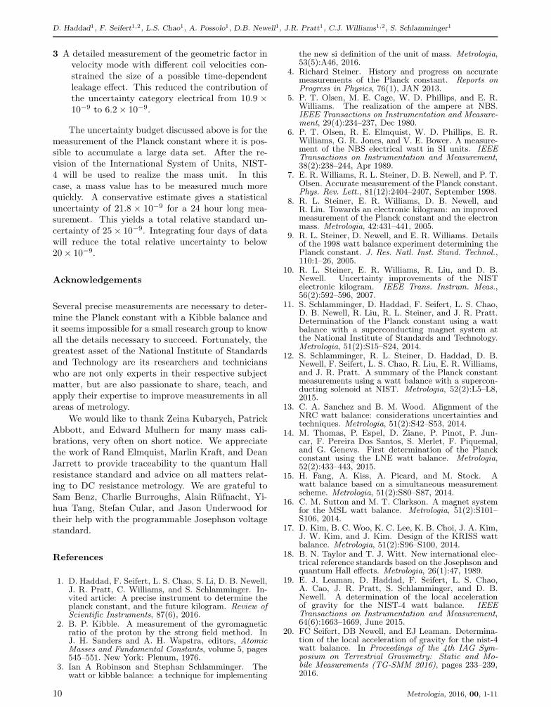
Figure 5. Measurements of the relative difference of thegeometric factor measured at velocity v from the geomet-ric factor measured at the nominal velocity. The errorbars denote the 1-σ statistical uncertainties associatedwith the measurements. The solid line is a least squaresfit with a constraint to pass through the point of nominalvelocity and ∆B = 0. The one sigma uncertainty intervalof the fit is given by the dashed lines surrounding the bestfit.

A time-dependent leakage resistance remains aconcern for the NIST-4 measurements. The possi-ble effect of the time-dependent storage of chargecan be assessed by measuring the geometric factorin velocity mode with different velocities of the coil.Changing the velocity changes the timing, in partic-ular how long the voltage is applied to various partsof the circuit. For example, the science data dis-cussed in Section 3. was taken with a nominal coilvelocity of vnom = 975µms−1. The total length ofthe sweep, including acceleration and deceleration is78mm. Hence, the voltage is applied on the coil for40 s before the coil reaches the weighing position. Re-ducing this velocity by a factor of two extends thetravel time by a factor of two.

To estimate the effect of the time-dependent leak-age on the measurement, we took a group of 30 sweepswith a velocity v 6= vnom bracketed by two groupsof 30 sweeps with vnom on either side. The analy-

sis of this set (= three groups) is done similarly tothe data analysis of the science data i.e., two parallelsecond degree polynomials were fitted to the mea-surements. The difference of the polynomials in Blis the result of one measurement. Many measure-ments were taken at 13 different velocities rangingfrom vnom/2 to 2vnom. Most of the measurementswere concentrated on the smallest and largest veloc-ity. Figure 5 shows the obtained differences in ∆Bl =Bl(v)−Bl(vvnom). A least squares adjustment of thedata to a straight line, ∆Bl/Bl = γ(v−vvnom) yieldsγ = (−2.76± 4.35)× 10−9mm−1 s.

This result agrees with zero within its uncertaintyand, thus, no correction to the data was applied.The relative uncertainty in h due to this effect formeasurements carried out with a nominal velocityof 975µms−1 is 4.24 × 10−9. Previously a value of10 × 10−9 was used for this line in the uncertaintybudget. This larger value was estimated from expe-riences with NIST-3. The time dependent leakage isa part of the electrical uncertainty. The relative un-certainty of this category reduces from 10.9×10−9 to6.2× 10−9.

5. Result and Discussion

Analysing 1174 sets taken between December 2015and April 2017, a final result of the Planck constant,

h = 6.626 069 934(89)× 10−34 J s, (22)

is obtained. This value corresponds to

hSI − h90h90

= (163± 13)× 10−9 (23)

The relative standard uncertainty of this resultis 13 × 10−9. The main categories of the uncer-tainty budget are listed in Table 1.1. For comparison,the uncertainties that were assigned for 2016 publi-cation [1] are also listed.

The new result includes the data that were usedto measure h in 2016 [1]. Superseding the 2016 value,the value reported here is relatively larger by 15 ×10−9. One reason for this increase is that the previousvalue included a relative correction of 17.5×10−9 dueto a change in the geometric factor in response tothe symmetric part of the weighing current. A moreprecise study showed that the change is only about1.4× 10−9 for a 1 kg mass standard.

The smaller uncertainty of the new measurementis due to the reduction of three line items in the un-certainty budget.

1 A new assessment of the statistical uncertaintythat was made possible by the larger data setgave an estimate of 3.0×10−9, about eight timessmaller than the original estimate of 24.9×10−9.

8 Metrologia, 2016, 00, 1-11


this measurement previous measurementSource item category item category

u/h× 109 u/h× 109 u/h× 109 u/h× 109

Calibration of resistor 4.5 4.5Time dependent leakage 4.2 10.0Leakage in velocity mode 0.7 0.7Leakage in force mode 0.5 0.5Josephson Voltage standard 0.3 0.3Grounding 0.0 0.0

Electrical 6.2 10.9Calibration of mass 5.7 5.5Transport 2.0 0.0Sorption 0.3 0.3Magnetic effects 0.3 3.0

Mass metrology 6.1 6.3Profile fitting 5.0 5.0Balance mechanics 5.0 5.0Laser verticality 4.3 5.4Field gradient 1.5 2.3Virtual power 1.2 2.7Abbe Offset 0.1 0.8

Alignment 4.7 6.5Statistical 2.5 2.5Site 2.1 2.1Water table 2.0 2.0Instrument 1.6 1.6Tie 1.0 1.0Vertical translation 0.6 0.6Additional corrections 0.2

Local acceleration, g 4.3 4.3Statistical 3.0 24.9Corrections for ∆I2 1.7 15.4Corrections for I 0.4 0.4Corrections for I2 0.2 0.2

Magnetic field 1.8 15.4Jitters in photo receivers 1.2 1.2Synchronization 1.0 1.0Diffraction 0.6 0.6Frequency leakage 0.4 0.4Wavelength 0.0 0.0Beam shear 0.0 0.0Time interval analyser timing 0.0 0.0

Velocity 1.7 1.7

Total relative uncertainty 13.5 33.6

Table 1.1 Sources of uncertainty and their relative magnitudes for measurements of h with the Kibble balance NIST-4.All entries are relative standard uncertainties (k = 1). Entries with 0.0 denote uncertainties that are smaller than0.05 × 10−9. Column two and three indicate the uncertainties in the present measurement and column four and fiveindicate the uncertainties in the previous measurement [1]. The lines in bold are categories which may consist of severalindividual items printed in regular font above the category. The categories as well as the items within are sorted bysize of the uncertainty in the present measurement.

2 A careful measurement of the influence of theweighing current on the geometric factor reduced

the uncertainty due to the magnetic field from15.4× 10−9 to 1.8× 10−9.

Metrologia, 2016, 00, 1-11 9


3 A detailed measurement of the geometric factor invelocity mode with different coil velocities con-strained the size of a possible time-dependentleakage effect. This reduced the contribution ofthe uncertainty category electrical from 10.9 ×10−9 to 6.2× 10−9.

The uncertainty budget discussed above is for themeasurement of the Planck constant where it is pos-sible to accumulate a large data set. After the re-vision of the International System of Units, NIST-4 will be used to realize the mass unit. In thiscase, a mass value has to be measured much morequickly. A conservative estimate gives a statisticaluncertainty of 21.8 × 10−9 for a 24 hour long mea-surement. This yields a total relative standard un-certainty of 25× 10−9. Integrating four days of datawill reduce the total relative uncertainty to below20× 10−9.

Acknowledgements

Several precise measurements are necessary to deter-mine the Planck constant with a Kibble balance andit seems impossible for a small research group to knowall the details necessary to succeed. Fortunately, thegreatest asset of the National Institute of Standardsand Technology are its researchers and technicianswho are not only experts in their respective subjectmatter, but are also passionate to share, teach, andapply their expertise to improve measurements in allareas of metrology.

We would like to thank Zeina Kubarych, PatrickAbbott, and Edward Mulhern for many mass cali-brations, very often on short notice. We appreciatethe work of Rand Elmquist, Marlin Kraft, and DeanJarrett to provide traceability to the quantum Hallresistance standard and advice on all matters relat-ing to DC resistance metrology. We are grateful toSam Benz, Charlie Burroughs, Alain Rufnacht, Yi-hua Tang, Stefan Cular, and Jason Underwood fortheir help with the programmable Josephson voltagestandard.

References

1. D. Haddad, F. Seifert, L. S. Chao, S. Li, D. B. Newell,J. R. Pratt, C. Williams, and S. Schlamminger. In-vited article: A precise instrument to determine theplanck constant, and the future kilogram. Review ofScientific Instruments, 87(6), 2016.

2. B. P. Kibble. A measurement of the gyromagneticratio of the proton by the strong field method. InJ. H. Sanders and A. H. Wapstra, editors, AtomicMasses and Fundamental Constants, volume 5, pages545–551. New York: Plenum, 1976.

3. Ian A Robinson and Stephan Schlamminger. Thewatt or kibble balance: a technique for implementing

the new si definition of the unit of mass. Metrologia,53(5):A46, 2016.

4. Richard Steiner. History and progress on accuratemeasurements of the Planck constant. Reports onProgress in Physics, 76(1), JAN 2013.

5. P. T. Olsen, M. E. Cage, W. D. Phillips, and E. R.Williams. The realization of the ampere at NBS.IEEE Transactions on Instrumentation and Measure-ment, 29(4):234–237, Dec 1980.

6. P. T. Olsen, R. E. Elmquist, W. D. Phillips, E. R.Williams, G. R. Jones, and V. E. Bower. A measure-ment of the NBS electrical watt in SI units. IEEETransactions on Instrumentation and Measurement,38(2):238–244, Apr 1989.

7. E. R. Williams, R. L. Steiner, D. B. Newell, and P. T.Olsen. Accurate measurement of the Planck constant.Phys. Rev. Lett., 81(12):2404–2407, September 1998.

8. R. L. Steiner, E. R. Williams, D. B. Newell, andR. Liu. Towards an electronic kilogram: an improvedmeasurement of the Planck constant and the electronmass. Metrologia, 42:431–441, 2005.

9. R. L. Steiner, D. Newell, and E. R. Williams. Detailsof the 1998 watt balance experiment determining thePlanck constant. J. Res. Natl. Inst. Stand. Technol.,110:1–26, 2005.

10. R. L. Steiner, E. R. Williams, R. Liu, and D. B.Newell. Uncertainty improvements of the NISTelectronic kilogram. IEEE Trans. Instrum. Meas.,56(2):592–596, 2007.

11. S. Schlamminger, D. Haddad, F. Seifert, L. S. Chao,D. B. Newell, R. Liu, R. L. Steiner, and J. R. Pratt.Determination of the Planck constant using a wattbalance with a superconducting magnet system atthe National Institute of Standards and Technology.Metrologia, 51(2):S15–S24, 2014.

12. S. Schlamminger, R. L. Steiner, D. Haddad, D. B.Newell, F. Seifert, L. S. Chao, R. Liu, E. R. Williams,and J. R. Pratt. A summary of the Planck constantmeasurements using a watt balance with a supercon-ducting solenoid at NIST. Metrologia, 52(2):L5–L8,2015.

13. C. A. Sanchez and B. M. Wood. Alignment of theNRC watt balance: considerations uncertainties andtechniques. Metrologia, 51(2):S42–S53, 2014.

14. M. Thomas, P. Espel, D. Ziane, P. Pinot, P. Jun-car, F. Pereira Dos Santos, S. Merlet, F. Piquemal,and G. Genevs. First determination of the Planckconstant using the LNE watt balance. Metrologia,52(2):433–443, 2015.

15. H. Fang, A. Kiss, A. Picard, and M. Stock. Awatt balance based on a simultaneous measurementscheme. Metrologia, 51(2):S80–S87, 2014.

16. C. M. Sutton and M. T. Clarkson. A magnet systemfor the MSL watt balance. Metrologia, 51(2):S101–S106, 2014.

17. D. Kim, B. C. Woo, K. C. Lee, K. B. Choi, J. A. Kim,J. W. Kim, and J. Kim. Design of the KRISS wattbalance. Metrologia, 51(2):S96–S100, 2014.

18. B. N. Taylor and T. J. Witt. New international elec-trical reference standards based on the Josephson andquantum Hall effects. Metrologia, 26(1):47, 1989.

19. E. J. Leaman, D. Haddad, F. Seifert, L. S. Chao,A. Cao, J. R. Pratt, S. Schlamminger, and D. B.Newell. A determination of the local accelerationof gravity for the NIST-4 watt balance. IEEETransactions on Instrumentation and Measurement,64(6):1663–1669, June 2015.

20. FC Seifert, DB Newell, and EJ Leaman. Determina-tion of the local acceleration of gravity for the nist-4watt balance. In Proceedings of the 4th IAG Sym-posium on Terrestrial Gravimetry: Static and Mo-bile Measurements (TG-SMM 2016), pages 233–239,2016.

10 Metrologia, 2016, 00, 1-11


21. A. D. Gillespie, K. Fujii, D. B. Newell, P. T. Olsen,A. Picard, R. L. Steiner, G. N. Stenbakken, and E. R.Williams. Alignment uncertainties of the NIST wattexperiment. IEEE Trans. Instrum. Meas., 46:605–608, 1997.

22. Mosteller F. and Tukey J. Data analysis and regres-sion. Addison-Wesley, 1977.

23. D. N. Politis, J. P. Romano, and M. Wolf. Subsam-pling. Springer-Verlag, New York, 1999.

24. P.J. Huber, J. Wiley, and W. InterScience. Robuststatistics. Wiley New York, 1981.

25. S. Schlamminger. Design of the permanent-magnetsystem for NIST-4. IEEE Transactions on Instru-mentation and Measurement, 62(6):1524–1530, June2013.

26. F. Seifert, A. Panna, S. Li, B. Han, L. Chao, A. Cao,D. Haddad, H. Choi, L. Haley, and S. Schlam-minger. Construction, measurement, shimming, andperformance of the NIST-4 magnet system. IEEETransactions on Instrumentation and Measurement,63(12):3027–3038, Dec 2014.

27. I A Robinson. Alignment of the npl mark iiwatt balance. Measurement Science and Technology,23(12):124012, 2012.

Received on None.

Metrologia, 2016, 00, 1-11 11

metrologia measurementoftheplanckconstantatthenational ... · metrologia...

Documents