methods to account for spatial autocorrelation in the ... · methods to account for spatial...
TRANSCRIPT
Methods to account for spatial autocorrelation in the analysisof species distributional data: a review
Carsten F. Dormann, Jana M. McPherson, Miguel B. Araujo, Roger Bivand, Janine Bolliger,Gudrun Carl, Richard G. Davies, Alexandre Hirzel, Walter Jetz, W. Daniel Kissling,Ingolf Kuhn, Ralf Ohlemuller, Pedro R. Peres-Neto, Bjorn Reineking, Boris Schroder,Frank M. Schurr and Robert Wilson
C. F. Dormann ([email protected]), Dept of Computational Landscape Ecology, UFZ Helmholtz Centre for EnvironmentalResearch, Permoserstr. 15, DE-04318 Leipzig, Germany. ! J. M. McPherson, Dept of Biology, Dalhousie Univ., 1355 Oxford StreetHalifax NS, B3H 4J1 Canada. !M. B. Araujo, Dept de Biodiversidad y Biologıa Evolutiva, Museo Nacional de Ciencias Naturales,CSIC, C/ Gutierrez Abascal, 2, ES-28006 Madrid, Spain, and Centre for Macroecology, Inst. of Biology, Universitetsparken 15, DK-2100 Copenhagen Ø, Denmark. ! R. Bivand, Economic Geography Section, Dept of Economics, Norwegian School of Economics andBusiness Administration, Helleveien 30, NO-5045 Bergen, Norway. ! J. Bolliger, Swiss Federal Research Inst. WSL, Zurcherstrasse111, CH-8903 Birmensdorf, Switzerland. ! G. Carl and I. Kuhn, Dept of Community Ecology (BZF), UFZ Helmholtz Centre forEnvironmental Research, Theodor-Lieser-Strasse 4, DE-06120 Halle, Germany, and Virtual Inst. Macroecology, Theodor-Lieser-Strasse 4, DE-06120 Halle, Germany. ! R. G. Davies, Biodiversity and Macroecology Group, Dept of Animal and Plant Sciences,Univ. of Sheffield, Sheffield S10 2TN, U.K. ! A. Hirzel, Ecology and Evolution Dept, Univ. de Lausanne, Biophore Building, CH-1015 Lausanne, Switzerland. !W. Jetz, Ecology Behavior and Evolution Section, Div. of Biological Sciences, Univ. of California, SanDiego, 9500 Gilman Drive, MC 0116, La Jolla, CA 92093-0116, USA. ! W. D. Kissling, Community and Macroecology Group,Inst. of Zoology, Dept of Ecology, Johannes Gutenberg Univ. of Mainz, DE-55099 Mainz, Germany, and Virtual Inst. Macroecology,Theodor-Lieser-Strasse 4, DE-06120 Halle, Germany. ! R. Ohlemuller, Dept of Biology, Univ. of York, PO Box 373, York YO105YW, U.K. ! P. R. Peres-Neto, Dept of Biology, Univ. of Regina, SK, S4S 0A2 Canada, present address: Dept of Biological Sciences,Univ. of Quebec at Montreal, CP 8888, Succ. Centre Ville, Montreal, QC, H3C 3P8, Canada. ! B. Reineking, Forest Ecology, ETHZurich CHN G 75.3, Universitatstr. 16, CH-8092 Zurich, Switzerland. ! B. Schroder, Inst. for Geoecology, Univ. of Potsdam, Karl-Liebknecht-Strasse 24-25, DE-14476 Potsdam, Germany. ! F. M. Schurr, Plant Ecology and Nature Conservation, Inst. ofBiochemistry and Biology, Univ. of Potsdam, Maulbeerallee 2, DE-14469 Potsdam, Germany. ! R. Wilson, Area de Biodiversidad yConservacion, Escuela Superior de Ciencias Experimentales y Tecnologıa, Univ. Rey Juan Carlos, Tulipan s/n, Mostoles, ES-28933Madrid, Spain.
Species distributional or trait data based on range map (extent-of-occurrence) or atlas survey data often displayspatial autocorrelation, i.e. locations close to each other exhibit more similar values than those further apart. Ifthis pattern remains present in the residuals of a statistical model based on such data, one of the key assumptionsof standard statistical analyses, that residuals are independent and identically distributed (i.i.d), is violated. Theviolation of the assumption of i.i.d. residuals may bias parameter estimates and can increase type I error rates(falsely rejecting the null hypothesis of no effect). While this is increasingly recognised by researchers analysingspecies distribution data, there is, to our knowledge, no comprehensive overview of the many available spatialstatistical methods to take spatial autocorrelation into account in tests of statistical significance. Here, wedescribe six different statistical approaches to infer correlates of species’ distributions, for both presence/absence(binary response) and species abundance data (poisson or normally distributed response), while accounting forspatial autocorrelation in model residuals: autocovariate regression; spatial eigenvector mapping; generalisedleast squares; (conditional and simultaneous) autoregressive models and generalised estimating equations. Acomprehensive comparison of the relative merits of these methods is beyond the scope of this paper. Todemonstrate each method’s implementation, however, we undertook preliminary tests based on simulated data.These preliminary tests verified that most of the spatial modeling techniques we examined showed good type Ierror control and precise parameter estimates, at least when confronted with simplistic simulated data containing
Ecography 30: 609!628, 2007doi: 10.1111/j.2007.0906-7590.05171.x
# 2007 The Authors. Journal compilation # 2007 Ecography
Subject Editor: Carsten Rahbek. Accepted 3 August 2007
609
spatial autocorrelation in the errors. However, we found that for presence/absence data the results andconclusions were very variable between the different methods. This is likely due to the low information contentof binary maps. Also, in contrast with previous studies, we found that autocovariate methods consistentlyunderestimated the effects of environmental controls of species distributions. Given their widespread use, inparticular for the modelling of species presence/absence data (e.g. climate envelope models), we argue that thiswarrants further study and caution in their use. To aid other ecologists in making use of the methods described,code to implement them in freely available software is provided in an electronic appendix.
Species distributional data such as species range maps(extent-of-occurrence), breeding bird surveys and bio-diversity atlases are a common source for analyses ofspecies-environment relationships. These, in turn, formthe basis for conservation and management plans forendangered species, for calculating distributions underfuture climate and land-use scenarios and other formsof environmental risk assessment.
The analysis of spatial data is complicated by aphenomenon known as spatial autocorrelation. Spatialautocorrelation (SAC) occurs when the values of vari-ables sampled at nearby locations are not independentfrom each other (Tobler 1970). The causes of spatialautocorrelation are manifold, but three factors areparticularly common (Legendre and Fortin 1989,Legendre 1993, Legendre and Legendre 1998): 1)biological processes such as speciation, extinction,dispersal or species interactions are distance-related; 2)non-linear relationships between environment and spe-cies are modelled erroneously as linear; 3) the statisticalmodel fails to account for an important environmentaldeterminant that in itself is spatially structured and thuscauses spatial structuring in the response (Besag 1974).The second and third points are not always referred to asspatial autocorrelation, but rather spatial dependency(Legendre et al. 2002). Since they also lead to auto-correlated residuals, these are equally problematic. Afourth source of spatial autocorrelation relates to spatialresolution, because coarser grains lead to a spatialsmoothing of data. In all of these cases, SAC mayconfound the analysis of species distribution data.
Spatial autocorrelation may be seen as both anopportunity and a challenge for spatial analysis. It is anopportunity when it provides useful information forinference of process from pattern (Palma et al. 1999)by, for example, increasing our understanding ofcontagious biotic processes such as population growth,geographic dispersal, differential mortality, socialorganization or competition dynamics (Griffith andPeres-Neto 2006). In most cases, however, the presenceof spatial autocorrelation is seen as posing a seriousshortcoming for hypothesis testing and prediction(Lennon 2000, Dormann 2007b), because it violatesthe assumption of independently and identically dis-tributed (i.i.d.) errors of most standard statisticalprocedures (Anselin 2002) and hence inflates type I
errors, occasionally even inverting the slope of relation-ships from non-spatial analysis (Kuhn 2007).
A variety of methods have consequently been devel-oped to correct for the effects of spatial autocorrelation(partially reviewed in Keitt et al. 2002, Miller et al. 2007,see below), but only a few have made it into theecological literature. The aims of this paper are to 1)present and explain methods that account for spatialautocorrelation in analyses of spatial data; the app-roaches considered are: autocovariate regression, spatialeigenvector mapping (SEVM), generalised least squares(GLS), conditional autoregressive models (CAR), simul-taneous autoregressive models (SAR), generalised linearmixed models (GLMM) and generalised estimationequations (GEE); 2) describe which of these methodscan be used for which error distribution, and discusspotential problems with implementation; 3) illustratehow to implement these methods using simulated datasets and by providing computing code (Anon. 2005).
Methods for dealing with spatialautocorrelation
Detecting and quantifying spatial autocorrelation
Before considering the use of modelling methods thataccount for spatial autocorrelation, it is a sensible firststep to check whether spatial autocorrelation is in factlikely to impact the planned analyses, i.e. if modelresiduals indeed display spatial autocorrelation. Check-ing for spatial autocorrelation (SAC) has become acommonplace exercise in geography and ecology (Sokaland Oden 1978a, b, Fortin and Dale 2005). Establishedprocedures include (Isaaks and Shrivastava 1989, Perryet al. 2002): Moran’s I plots (also termed Moran’s Icorrelogram by Legendre and Legendre 1998), Geary’sc correlograms and semi-variograms. In all three cases ameasure of similarity (Moran’s I, Geary’s c) or variance(variogram) of data points (i and j) is plotted as afunction of the distance between them (dij). Distancesare usually grouped into bins. Moran’s I-based correlo-grams typically show a decrease from some level of SACto a value of 0 (or below; expected value in the absenceof SAC: E(I)"#1/(n!1), where n"sample size),indicating no SAC at some distance between locations.Variograms depict the opposite, with the variance
610
between pairs of points increasing up to a certaindistance, where variance levels off. Variograms are morecommonly employed in descriptive geostatistics, whilecorrelograms are the prevalent graphical presentation inecology (Fortin and Dale 2005).
Values of Moran’s I are assessed by a test statistic(the Moran’s I standard deviate) which indicates thestatistical significance of SAC in e.g. model residuals.Additionally, model residuals may be plotted as a mapthat more explicitly reveals particular patterns of spatialautocorrelation (e.g. anisotropy or non-stationarity ofspatial autocorrelation). For further details and for-mulae see e.g. Isaaks and Shrivastava (1989) or Fortinand Dale (2005).
Assumptions common to all modellingapproaches considered
All methods assume spatial stationarity, i.e. spatialautocorrelation and effects of environmental correlatesto be constant across the region, and there are very fewmethods to deal with non-stationarity (Osborne et al.2007). Stationarity may or may not be a reasonableassumption, depending, among other things, on thespatial extent of the study. If the main cause of spatialautocorrelation is dispersal (for example in research onanimal distributions), stationarity is likely to beviolated, for example when moving from a floodplainto the mountains, where movement may be morerestricted. One method able to accommodate spatialvariation in autocorrelation is geographically weightedregression (Fotheringham et al. 2002), a method notconsidered here because of its limited use for hypothesistesting (coefficient estimates depend on spatial position)and because it was not designed to remove spatialautocorrelation (see e.g. Kupfer and Farris 2007, for aGWR correlogram).
Another assumption is that of isotropic spatialautocorrelation. This means that the process causingthe spatial autocorrelation acts in the same way in alldirections. Environmental factors that may causeanisotropic spatial autocorrelation are wind (giving awind-dispersed organism a preferential direction), watercurrents (e.g. carrying plankton), or directionality insoil transport (carrying seeds) from mountains to plains.He et al. (2003) as well as Worm et al. (2005) provideexamples of analyses accounting for anisotropy inecological data, and several of the methods describedbelow can be adapted for such circumstances.
Description of spatial statistical modellingmethods
The methods we describe in the following fall broadlyinto three groups. 1) Autocovariate regression and
spatial eigenvector mapping seek to capture the spatialconfiguration in additional covariates, which are thenadded into a generalised linear model (GLM). 2)Generalised least squares (GLS) methods fit a var-iance-covariance matrix based on the non-independenceof spatial observations. Simultaneous autoregressivemodels (SAR) and conditional autoregressive models(CAR) do the same but in different ways to GLS, andthe generalised linear mixed models (GLMM) weemploy for non-normal data are a generalisation ofGLS. 3) Generalised estimating equations (GEE) splitthe data into smaller clusters before also modelling thevariance-covariance relationship. For comparison, thefollowing non-spatial models were also employed:simple GLM and trend-surface generalised additivemodels (GAM: Hastie and Tibshirani 1990, Wood2006), in which geographical location was fitted usingsplines as a trend-surface (as a two-dimensional splineon geographical coordinates). Trend surface GAM doesnot address the problem of spatial autocorrelation, butmerely accounts for trends in the data across largergeographical distances (Cressie 1993). A promising toolwhich became available only recently is the use ofwavelets to remove spatial autocorrelation (Carl andKuhn 2007b). However, the method was published toorecently to be included here and hence awaits furthertesting.
We also did not include Bayesian spatial models inthis review. Several recent publications have employedthis method and provide a good coverage of itsimplementation (Osborne et al. 2001, Hooten et al.2003, Thogmartin et al. 2004, Gelfand et al. 2005,Kuhn et al. 2006, Latimer et al. 2006). The Bayesianapproach to spatial models used in these studies is basedeither on a CAR or an autologistic implementationsimilar to the one we used as a frequentist method. TheBayesian framework allows for a more flexible incor-poration of other complications (observer bias, missingdata, different error distributions) but is much morecomputer-intensive then any of the methods presentedhere.
Beyond the methods mentioned above, there arealso those which correct test statistics for spatial auto-correlation. These include Dutilleul’s modified t-test(Dutilleul 1993) or the CRH-correction for correla-tions (Clifford et al. 1989), randomisation tests such aspartial Mantel tests (Legendre and Legendre 1998), orstrategies employed by Lennon (2000), Liebhold andGurevitch (2002) and Segurado et al. (2006) which areall useful as a robust assessment of correlation betweenenvironmental and response variables. As these methodsdo not allow a correction of the parameter estimates,however, they are not considered further in this study.In the following sections we present a detailed descrip-tion of all methods employed here.
611
1. Autocovariate models
Autocovariate models address spatial autocorrelation byestimating how much the response variable at any onesite reflects response values at surrounding sites. This isachieved through a simple extension of generalisedlinear models by adding a distance-weighted function ofneighbouring response values to the model’s explana-tory variables. This extra parameter is known as theautocovariate. The autocovariate is intended to capturespatial autocorrelation originating from endogenousprocesses such as conspecific attraction, limited dis-persal, contagious population growth, and movementof censused individuals between sampling sites (Smith1994, Keitt et al. 2002, Yamaguchi et al. 2003).
Adding the autocovariate transforms the linearpredictor of a generalised linear model from its usualform, y"Xb!o, to y"Xb$rA!o, where b is avector of coefficients for intercept and explana-tory variables X; and r is the coefficient of the autoco-variate A.
A at any site i may be calculated as:
Ai"X
j ! ki
wijyj (the weighted sum) or
Ai"
X
j ! ki
wijyjX
j ! ki
wij
(the weighted average);
where yj is the response value of y at site j among site i’sset of ki neighbours; and wij is the weight given to sitej’s influence over site i (Augustin et al. 1996, Gumpertzet al. 1997). Usually, weight functions are related togeographical distance between data points (Augustinet al. 1996, Araujo and Williams 2000, Osborne et al.2001, Brownstein et al. 2003) or environmentaldistance (Augustin et al. 1998, Ferrier et al. 2002).The weighting scheme and neighbourhood size (k) areoften chosen arbitrarily, but may be optimised (by trialand error) to best capture spatial autocorrelation(Augustin et al. 1996). Alternatively, if the cause ofspatial autocorrelation is known (or at least suspected),the choice of neighbourhood configuration may beinformed by biological parameters, such as the species’dispersal capacity (Knapp et al. 2003).
Autocovariate models can be applied to binomialdata (‘‘autologistic regression’’, Smith 1994, Augustinet al. 1996, Klute et al. 2002, Knapp et al. 2003), aswell as normally and Poisson-distributed data (Luotoet al. 2001, Kaboli et al. 2006).
Where spatial autocorrelation is thought to beanisotropic (e.g. because seed dispersal follows prevail-ing winds or downstream run-off), multiple autoco-variates can be used to capture spatial autocorrelation indifferent geographic directions (He et al. 2003).
2. Spatial eigenvector mapping (SEVM)
Spatial eigenvector mapping is based on the idea thatthe spatial arrangement of data points can be translatedinto explanatory variables, which capture spatial effectsat different spatial resolutions. During the analysis,those eigenvectors that reduce spatial autocorrelation inthe residuals best are chosen explicitly as spatialpredictors. Since each eigenvector represents a particu-lar spatial patterning, SAC is effectively allowed to varyin space, relaxing the assumption of both spatialisotropy and stationarity. Plotting these eigenvectorsreveals the spatial patterning of the spatial autocorrela-tion (see Diniz-Filho and Bini 2005, for an example).This method could thus be very useful for data withSAC stemming from larger scale observation bias.
The method is based on the eigenfunction decom-position of spatial connectivity matrices, a relativelynew and still unfamiliar method for describing spatialpatterns in complex data (Griffith 2000b, Borcard andLegendre 2002, Griffith and Peres-Neto 2006, Drayet al. 2006). A very similar approach, called eigenvectorfiltering, was presented by Diniz-Filho and Bini (2005)based on their method to account for phylogenetic non-independence in biological data (Diniz-Filho et al.1998). Eigenvectors from these matrices represent thedecompositions of Moran’s I statistic into all mutuallyorthogonal maps that can be generated from a givenconnectivity matrix (Griffith and Peres-Neto 2006).Either binary or distance-based connectivity matricescan be decomposed, offering a great deal of flexibilityregarding topology and transformations. Given thenon-Euclidean nature of the spatial connectivity ma-trices (i.e. not all sampling units are connected), bothpositive and negative eigenvalues are produced. Thenon-Euclidean part is introduced by the fact that onlycertain connections among sampling units, and not all,are considered. Eigenvectors with positive eigenvaluesrepresent positive autocorrelation, whereas eigenvectorswith negative eigenvalues represent negative autocorre-lation. For the sake of presenting a general method thatwill work for either binary or distance matrices, we useda distance-based eigenvector procedure (after Drayet al. 2006) which can be summarized as follows:1) compute a pairwise Euclidean (geographic) distancematrix among sampling units: D"[dij]; 2) choose athreshold value t and construct a connectivity matrixusing the following rule:
W"[wij]"0 if i" j0 if dij" t
[1#(dij=4t)2] if dij5 t
8
<
:
where t is chosen as the maximum distance thatmaintains connections among all sampling units beingconnected using a minimum spanning tree algorithm
612
(Legendre and Legendre 1998). Because the exampledata we use represent a regular grid (see below), t"1 andthus wij is either 0 or 1!1/42"0.9375 in our analysis.Note that we can change 0.9375 to 1 without affectingeigenvector extraction. This would make the matrix fullycompatible with a binary matrix which is the case for aregular grid. 3) Compute the eigenvectors of the centredsimilarity matrix: (I!11T/n)W(I!11T/n), where I is theidentity matrix. Due to numerical precision regardingthe eigenvector extraction of large matrices (Bai et al.1996) the method is limited to ca 7000 observationsdepending on platform and software (but see Griffith2000a, for solutions based on large binary connectivitymatrices). 4) Select eigenvectors to be included as spatialpredictors in a linear or generalised linear model. Here, amodel selection procedure that minimizes the amount ofspatial autocorrelation in residuals was used (see Griffithand Peres-Neto 2006 and Appendix for computationaldetails). In this approach, eigenvectors are added to amodel until the spatial autocorrelation in the residuals,measured by Moran’s I, is non-significant. Our selectionalgorithm considered global Moran’s I (i.e. autocorrela-tion across all residuals), but could be easily amended totarget spatial autocorrelation within certain distanceclasses. The significance of Moran’s I was tested using apermutation test as implemented in Lichstein et al.(2002). This potentially renders the selection procedurecomputationally intensive for large data sets (200 ormore observations), because a permutation test must beperformed for each new eigenvector entered into themodel. Once the location-dependent, but data-inde-pendent eigenvectors are selected, they are incorporatedinto the ordinary regression model (i.e. linear orgeneralized linear model) as covariates. Since theirrelevance has been assessed during the filtering processmodel simplification is not indicated (although someeigenvectors will not be significant).
3. Spatial models based on generalised leastsquares regression
In linear models of normally distributed data, spatialautocorrelation can be addressed by the related ap-proaches of generalised least squares (GLS) and auto-regressive models (conditional autoregressive models(CAR) and simultaneous autoregressive models (SAR)).GLS directly models the spatial covariance structure inthe variance-covariance matrix a, using parametricfunctions. CAR and SAR, on the other hand, modelthe error generating process and operate with weightmatrices that specify the strength of interaction betweenneighbouring sites.
Although models based on generalised least squareshave been known in the statistical literature fordecades (Besag 1974, Cliff and Ord 1981), their
application in ecology has been very limited so far(Jetz and Rahbek 2002, Keitt et al. 2002, Lichsteinet al. 2002, Dark 2004, Tognelli and Kelt 2004). Thisis most likely due to the limited availability ofappropriate software that easily facilitates the applica-tion of these kinds of models (Lichstein et al. 2002).With the recent development of programs that fit avariety of GLS (Littell et al. 1996, Pinheiro and Bates2000, Venables and Ripley 2002) and autoregressivemodels (Kaluzny et al. 1998, Bivand 2005, Rangelet al. 2006), however, the range of available tools forecologists to analyse spatially autocorrelated normaldata has been greatly expanded.
Generalised least squares (GLS)As before, the underlying model is Y"Xb!o, with theerror vector o"N(0,aa). aa is called the variance-covariance matrix. Instead of fitting individual valuesfor the variance-covariance matrix aa, a parametriccorrelation function is assumed. Correlation functionsare isotropic, i.e. they depend only on the distance sijbetween locations i and j, but not on the direction.Three frequently used examples of correlation functionsC(s) also used in this study are exponential (C(s)"s2
exp(#r/s)), Gaussian (C(s)"s2 exp(#r/s))2) and sphe-rical (C(s)"s2(1#2=p(r=s
!!!!!!!!!!!!!!!!!!
1#r2=s2p
$sin#1r=s));where r is a scaling factor that is estimated from thedata).
Some restrictions are placed upon the resultingvariance-covariance matrix a: a) it must be symmetric,and b) it must be positive definite. This guarantees thatthe matrix is invertible, which is necessary forthe fitting process (see below). The choice of correlationfunction is commonly based on a visual investigation ofthe semi-variogram or correlogram of the residuals.
Parameter estimation is a two-step process. First, theparameters of the correlation function (i.e. scalingfactor r in the examples used here) are found byoptimizing the so called profiled log-likelihood, whichis the log-likelihood where the unknown values for band s2 are replaced by their algebraic maximumlikelihood estimators. Secondly, given the parameter-ization of the variance-covariance matrix, the values forb and s2 are found by solving a weighted ordinary leastsquare problem:
"
XX#1=2#T
y""
XX#1=2#T
Xb$"
XX#1=2#T
o
where the error term (aa#1=2)To is now normallydistributed with mean 0 and variance s2I.
Autoregressive modelsBoth CAR and SAR incorporate spatial autocorrelationusing neighbourhood matrices which specify the
613
relationship between the response values (in the case ofCAR) or residuals (in the case of SAR) at each location(i) and those at neighbouring locations (j) (Cressie1993, Lichstein et al. 2002, Haining 2003). Theneighbourhood relationship is formally expressed in an%n matrix of spatial weights (W) with elements (wij)representing a measure of the connection betweenlocations i and j. The specification of the spatial weightsmatrix starts by identifying the neighbourhood struc-ture of each cell. Usually, a binary neighbourhoodmatrix N is formed where nij"1 when observation j is aneighbour to observation i. This neighbourhood can beidentified by the adjacency of cells on a grid map, or byEuclidean or great circle distance (e.g. the distancealong earth’s surface), or predefined according to aspecific number of neighbours (e.g. a neighbourhooddistance of 1.5 in our case includes the 8 adjacentneighbours). The elements of N can further be weightedto give closer neighbours higher weights and moredistant neighbours lower weights. The matrix of spatialweights W consists of zeros on the diagonal, andweights for the neighbouring locations (wij) in the off-diagonal positions. A good introduction to the CARand SAR methodology is given by Wall (2004).
Conditional autoregressive models (CAR)The CAR model can be written as (Keitt et al. 2002):
Y"Xb$rW (Y#Xb)$o
with o"N(0, Vc). If s2i "s2 for all locations i, the
covariance matrix is VC"s2 (I#rW)#1, where Whas to be symmetric. Consequently, CAR is unsuitablewhen directional processes such as stream flow effects orprevalent wind directions are coded as non-Euclideandistances, resulting in an asymmetric covariance matrix.In such situations, the closely related simultaneousautoregressive models (SAR) are a better option, as theirW need not be symmetric (see below). For our analysis,we used a row-standardised binary weights matrix for aneighbour-distance of 2 (Appendix).
Simultaneous autogressive models (SAR)SAR models can take three different forms (we use thenotation presented in Anselin 1988), depending onwhere the spatial autoregressive process is believed tooccur (see Cliff and Ord 1981, Anselin 1988, Haining2003, for details). The first SAR model assumes that theautoregressive process occurs only in the responsevariable (‘‘lagged-response model’’), and thus includesa term (rW) for the spatial autocorrelation in theresponse variable Y, but also the standard term for thepredictors and errors (Xb$o) as used in an ordinaryleast squares (OLS) regression. Spatial autocorrelationin the response may occur, for example, where
propagules disperse passively with river flow, leadingto a directional spatial effect. The SAR lagged-responsemodel (SAR lag) takes the form
Y"rWY$Xb$o
(which is equivalent to Y"(I#rW)#1Xb$(I#rW)#1o), where r is the autoregression parameter,W the spatial weights matrix, and b a vector represent-ing the slopes associated with the predictors in theoriginal predictor matrix X.
Second, spatial autocorrelation can affect bothresponse and predictor variables (‘‘lagged-mixedmodel’’, SAR mix). Ecologically, this adds a localaggregation component to the spatial effect in the lag-model above. In this case, another term (WXg) mustalso appear in the model, which describes the regressioncoefficients (g) of the spatially lagged predictors (WX).The SAR lagged-mixed model takes the form
Y"rWY$Xb$WXg$o
Finally, the ‘‘spatial error model’’ (SAR err) assumesthat the autoregressive process occurs only in the errorterm and neither in response nor in predictor variables.The model is most similar to the CAR, with nodirectionality in the error. In this case, the usual OLSregression model (Y"Xb$o) is complemented by aterm (lWm) which represents the spatial structure (lW)in the spatially dependent error term (m). The SARspatial error model thus takes the form
Y"Xb$lWm$o
where l is the spatial autoregression coefficient, and therest as above. SAR and CAR are related to each other,but the terms rW used in both CAR and SAR are notidentical. As noted above, in CAR, W must besymmetrical, whereas in SAR it need not be. Let rWof the CAR be called K and rW of the SAR be called S.Then any SAR is a CAR with K"S$ST#STS(Haining 2003). Assuming constant variance s2, theformal relationship between the error variance-covar-iance matrices in GLS, SAR, and CAR is as follows:VGLS"s2C(s); VCAR"s2 (I!K)#1and VSAR"s2 (I!S)#1(I!ST)#1, with K and S as defined above. ThusCAR and SAR models are equivalent if VCAR"VSAR.The relationship between specific values in correlationmatrix C and weight matrix W is not straightforward,however. In particular, spatial dependence parametersthat decrease monotonically with distance do notnecessarily correspond to spatial covariances that de-crease monotonically with distance (Waller and Gotway2004). An extensive comparison of the impact ofdifferent model formulations on parameter estimationand type I error control is given by Kissling and Carl(2007) using simulated datasets with different spatialautocorrelation structures.
614
Spatial generalised linear mixed models (GLMM)Spatial generalised linear mixed models are generalisedlinear models (GLMs) in which the linear predictormay contain random effects and within-group errorsmay be spatially autocorrelated (Breslow and Clayton1993, Venables and Ripley 2002). Formally, if Yij isthe j-th observation of the response variable in group i,
E[Yijjzi]"g#1(hij) and hij"xijb$zijzi;
where g is the link function, h is the linear predictor, band z are coefficients for fixed and random effects,respectively, and x and z are the explanatory variablesassociated with these effects. Conditional on therandom effects z, the standard GLM applies and thewithin-group distribution of Y can be described usingthe same error distributions as in GLM.
Since the GLMM is often implemented based onso-called penalized quasi-likelihood (PQL) methods(Breslow and Clayton 1993, Venables and Ripley2002) around the GLS-algorithm (McCullough andNelder 1989), we can use it in a similar way, i.e. fittingthe structure of the variance-covariance-matrix to thedata (see GLS above), albeit with a different errordistribution. In cases where spatial data are availablefrom several disjunct regions, GLMMs can thus be usedto fit overall fixed effects while spatial correlationstructures are nested within regions, allowing theaccommodation of regional differences in e.g. auto-correlation distances, and assuming autocorrelationonly between observations within the same region(Orme et al. 2005, Davies et al. 2006, Stephensonet al. 2006).
4. Spatial generalised estimating equations (GEE)
Liang and Zeger (1986) developed the generalisedestimating equation (GEE) approach which is anextension of generalised linear models (GLMs). Whenresponses are measured repeatedly through time orspace, the GEE method takes correlations withinclusters of sampling units into account by means of aparameterised correlation matrix, while correlationsbetween clusters are assumed to be zero. In a spatialcontext such clusters can be interpreted as geographicalregions, if distances between different regions are largeenough (Albert and McShane 1995). We modified theapproach of Liang and Zeger to use these GEE modelsfor spatial, two-dimensional datasets sampled in rec-tangular grids (see Carl and Kuhn 2007a, for moredetails). Fortunately, estimates of regression parametersare fairly robust against misspecification of the correla-tion matrix (Dobson 2002). The GEE approach isespecially suited for parameter estimation rather thanprediction (Augustin et al. 2005).
Firstly, consider the generalised linear model E(y)"m, m"g#1 (Xb) where y is a vector of responsevariables, m the expected value, g#1 the inverse of thelink function, X the matrix of predictors, and b thevector of regression parameters. Minimization of aquadratic form leads to the GLM score equation(Diggle et al. 1995, Dobson 2002, Myers et al. 2002)
DTV#1(y#m)"0;
where DT is the transposed matrix of D of partialderivatives D"1m/1b. Secondly, note that the varianceof the response can be replaced by a variance-covariancematrix V which takes into account that observationsare not independent. In GEEs, the sample is split upinto m clusters and the complete dataset is ordered in away that in all clusters data are arranged in the samesequence: E(yj)"mj ; mj"g#1(Xj b): Then the var-iance-covariance matrix has block diagonal form, sinceresponses of different clusters are assumed to beuncorrelated. One can consequently transform the scoreequation into the following form
X
m
j"1
DTj V
#1j (yj#m j)"0;
which sums over all clusters j. This equation is calledthe generalised estimating equation or the quasi-scoreequation.
For spatial dependence the following correlationstructures for V are important: 1) Fixed. The correla-tion structure is completely specified by the user andwill not change during an iterative procedure. Referredto here as GEE. 2) User defined. Correlation para-meters are to be estimated, but one can specify thatcertain parameters must be equal, e.g. that the strengthof correlation is always the same at a certain distance.Referred to here as geese.
First, we consider the GEE model with fixedcorrelation structure. In order to predetermine thecorrelation structure we have good reasons to assumethat the correlation decreases exponentially with in-creasing spatial distance in ecological applications.Therefore, we use the function
a"adij1
for computation of correlation parameters a. Here dij isthe distance between centre points of grid cells i and jand a1 is the correlation parameter for nearestneighbours. The parameter a1 is estimated by Moran’sI of GLM residuals. In this way we obtain a full n%ncorrelation matrix with known parameters. Thusclustering is not necessary.
In the user defined case we build a specific variance-covariance matrix in block diagonal form with 5unknown correlation parameters (corresponding tothe five different distance classes in a 3%3 grid) which
615
have to be calculated iteratively. The dispersion para-meter as a correction of overdispersion can be calculatedas well.
Example analysis using simulated data
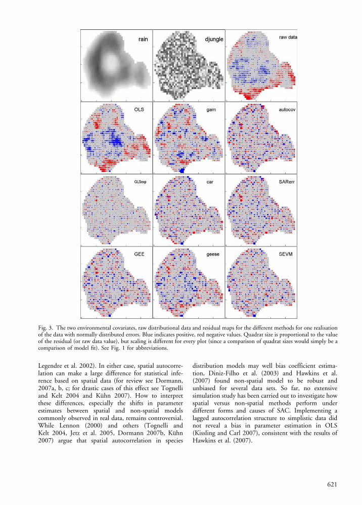
To illustrate and compare the various approaches thatare available to incorporate SAC into the analysis ofspecies distribution data, we constructed artificialdatasets with known properties. The datasets representvirtual species distribution data (for example speciesatlases) and environmental (such as climatic) covariates,available on a lattice of 1108 square cells imposed onthe surface of a virtual island (Fig. 3).
Generation of artificial distribution data
The basis for the virtual island is a subset of the volcanodata set in R, which consists of a digital elevation modelfor Auckland’s Maunga Whau Volcano in New Zealand(Anon. 2005). Two uncorrelated (Pearson’s r"0.013,p"0.668) environmental variables were created basedon the altitude-component of this data set: ‘‘rain’’ and‘‘djungle’’. These data are available as electronicappendix and are depicted in Fig. 3. While ‘‘rain’’ isa rather deterministic function of altitude (including arain-shadow in the east), ‘‘djungle’’ is dominated by ahigh noise component. Data are given in the Appendix.
On this lattice the species distribution data, yi (with ian indicator for cell (i"1, 2 . . ., 1108)), were simulatedas a function of one of the two artificial environmentalpredictors, raini. Onto this functional relationship, weadded a spatially correlated noise component we refer toas error oi. The covariate raini can for example bethought of as estimates of the total annual amount ofrainfall in cell i. We simulated the three mostcommonly available types of species distribution data;continuous, binary and count data, using the normaldistribution and approximations of the Poisson andbinomial distributions respectively. The followingmodels were used to simulate the artificial data: 1)normally distributed data: yi"80#0.015%raini$10%oi. 2) Binary data: yi"0 if piB0.5, and yi"1if, pi ]0.5, where pi"qi$
!!!!!!!!!!!!!!!!!!!
qi(1#qi)p
oi; and
/qi"e3#0:003&raini
1$ e3#0:003&raini
: 3) Poisson data: /yi"round(ki$!!!!
ki
p
oi); where /ki"e3#0:001&raini ; and round is an operatorused to round values to the nearest integer. This led tosimulated data with no over- or underdispersion.
A weight matrixW was used to simulate the spatiallycorrelated errors oi using weights according to thedistance between data points. Let D"(dij) be the(Euclidean) distance matrix for the distances between
cells i and j (dij"0 if i"j). On our lattice, the distancebetween the mid-points of neighbouring cells is dij"1.Then, V"(vij) is a matrix defined as vij"exp(#r%dij); r (r]0) is a parameter that determines thedecline of inter-cell correlation in errors with inter-cell distance. The strength of spatial autocorrelationincreases with increasing values of r (there is no spatialautocorrelation if r"0). Here, we used a value of r"0.3, which resulted in strongly correlated errors inneighbouring cells (vij"0.74, if dij"1), but a steepdecline of autocorrelation with increasing distance. Aweights matrix W was calculated (by Choleski decom-position) using V"WTW. Finally, the spatially corre-lated errors are given by o"WTj, with j drawn fromthe standard normal distribution.
Analysis of simulated data
For each error distribution, ten data sets were created,each using a random realisation of the spatiallyautocorrelated errors, using random draws of ji. Thesedata sets were then submitted to statistical analyses inwhich the response variables were modelled using anumber of different linear models for the normallydistributed data, and generalized linear models with thebinomial distribution and logit-link for the binary data,and Poisson distribution and log-link for the countdata: E(yi)"g#1(a$b%raini$g%djunglei), where gare the corresponding link functions (identity for thenormal distribution). The variable ‘‘djungle’’ wasentered into all of the statistical models as an additionalpredictor of the response. This was done to be able toassess the models’ ability to distinguish random noisefrom meaningful variables.
Simulations and analyses were primarily carried out(see Appendix for implementation details and R-code)using the statistical programming software R (Anon.2005), with packages gee (Carey 2002), geepack (Yan2002, 2004), spdep (Bivand 2005), ncf (Bjørnstad andFalck 2000) and MASS (Venables and Ripley 2002).Calculations for the spatial eigenvector mapping wereoriginally performed in Matlab using routines laterported to R (spdep) by Roger Bivand and Pedro Peres-Neto. Additional functions (Appendix) to work gen-eralised estimating equations on a 2-D lattice werewritten by Gudrun Carl (Carl and Kuhn 2007a). Seealso Table 1 for alternative software.
As most of the statistical methods tested allow forsome flexibility in the precise structure of their spatialcomponent, several models per method were calculatedfor each simulated dataset. This allowed us to identifythe model configuration that most successfully ac-counted for spatial autocorrelation in the data athand, by, for example, varying the distance over whichspatial autocorrelation was assumed to occur, or its
616

functional form. Inferior models were discarded, so thatthe results section below reports only on the bestconfiguration for each approach. We used residualsbased on fitted values and which were as such calculatedfrom both the spatial and the non-spatial modelcomponents. For each, we report the following details:1) model coefficients (and their standard errors); sincethe true parameters are known, we can directly judgethe quality of coefficient estimation; 2) removal of SAC(global Moran’s I, i.e. Moran’s I computed acrossneighbourhood up to a distance of 20, and correlo-grams, which plot Moran’s I for different distanceclasses); 3) spatial distribution of residuals (map).
Results of simulations
It is worth pointing out that the main aim of this studyis to illustrate the different methods by applying themto the same data sets. The ten realisations of one type ofspatial autocorrelation do not allow us to provide acomprehensive evaluation of the relative merits of eachof the methods considered. Such evaluation is beyondthe scope of this review paper, and will depend on thedata set and question under study. Nonetheless, someinteresting results emerged from our simulations.
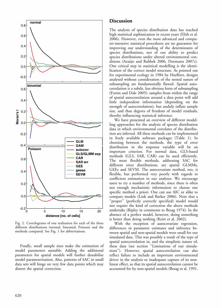
Spatial and non-spatial models differed conside-rably in terms of the spatial signature in their residuals(Table 2; Fig. 2 and 3). Residual maps for OLS/GLMand GAM exhibit clusters of large residuals of the samesign (Fig. 3), indicating that these models were not able
to remove all spatial autocorrelation from the data. Inour case we know that this is due neither to theomission of an important variable nor an incorrectfunctional relationship, but a simulated aggregationmechanism in the errors. In comparison, all spatialmodels managed to decrease spatial autocorrelation inthe residuals (Fig. 2), although not all were able tocompletely eliminate it. Geese performed worst in thisregard. Our simulations are not comprehensive enough,however, to allow us to deduce what the influence ofthis incomplete removal of SAC might be on parameterestimation or hypothesis testing.
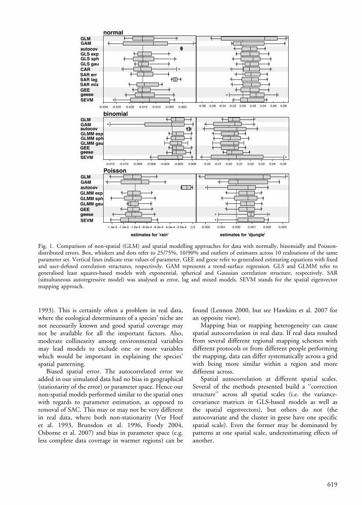
Another ! though inconsistent ! difference betweenthe spatial and non-spatial models especially withbinary data was that standard errors of the coefficientestimates for ‘‘rain’’ and ‘‘djungle’’ were often larger forthe spatial models (Fig. 1). For normal and Poissondata, differences in coefficient estimates between spatialand non-spatial models were relatively small, andstatistical inference was not affected. Only autocovariatemodel and SAR lag provided consistently incorrectestimates of the spatially autocorrelated parameter‘‘rain’’.
Most model approaches performed well with respectto type I and II error rates for the normal and Poissondata, correctly identifying ‘‘rain’’ as a significant effect(Table 2). An exception was autocovariate regression,which severely and consistently underestimated theeffects of rain (Table 2, Fig. 1). Model performancewas worse for data with a binomial error structure thanfor models with normal or Poisson error structure.
Table 1. Methods correcting for spatial autocorrelation and their software implementations. This list is not exhaustive but representsthe major software developments in use.
Method R-package1 Computational intensity2 Other3
Autocovariate regression spdep lowAutoregressive models4 (CAR, SAR) spdep medium GeoDa, Matlab*, SAM, SpaceStat, S-plus$Bayesian analysis very high WinBUGS/GeoBUGSGeneralised linear mixed model MASS very high SAS (glimmix)Generalised estimating equations gee, geepack low SASGeneralised least squares4 MASS, nlme high SAS, SAMSpatial eigenvector mapping spdep very high Matlab, SAM
1 for most R-packages (Bhttp://www.r-project.org") an equivalent for S-plus is available.2 low, medium, high and very high refer roughly to a few seconds, several minutes, a few hours and several hours of CPU-time permodel (1108 data points on a Pentium 4 dual core, 3.8GHz, 2GB RAM).3 GeoDa: freeware: Bhttp://www.geoda.uiuc.edu".4 for normally distributed error only.Matlab: Bhttp://www.mathworks.com", with EigMapSel ! a matlab compiled software to perform the eigenvector selectionprocedure for generalised linear models (normal, logistic and poisson) ! available in ESA’s Electronic Data Archive (Griffith andPeres-Neto 2006).SAM: spatial analysis for macroecology; freeware under: Bhttp://www.ecoevol.ufg.br/sam/".SAS: statistical analysis system; commercial software: Bhttp://www.sas.com".SpaceStat: commercial software: Bhttp://www.terraseer.com/products/spacestat.html".S-plus: commercial software: Bhttp://www.insightful.com".WinBUGS/GeoBUGS: freeware: Bhttp://www.mrc-bsu.cam.ac.uk/bugs/winbugs/contents.shtml".*requires the free ‘‘Spatial Econometric toolbox’’: Bhttp://www.spatial-econometrics.com".$requires additional module ‘‘spatial’’.
617
When applied to such data, autocovariate regression (9false negatives) and GAM (3 false negatives) were ratherprone to type II errors (results not shown). Moreover,the spurious effect of djungle would have been retainedin the model in several cases (based on a signi-ficance level of a"0.05: 6 normal, 2 binomial and 1Poisson model of those presented in Table 2), resultingin type I errors (rejecting a null hypothesis although itwas true).
The ability of simultaneous autoregressive models(SAR) to correctly estimate parameters dependedheavily on SAR model structure. For instance, using alagged response model in our artificial dataset yieldedmuch poorer coefficient estimates for ‘‘rain’’ than usingan error model (Fig. 1). This was to be expected, sinceour artificial distribution data was created such that itsspatial structure most closely resembled that of the SARerror model.
We used an exponential distance decay function togenerate the spatial error (see above). Hence, we wouldalso expect those methods to perform best in which acorrelation function can be defined accordingly(i.e. GLS, GLMM and GEE). While indeed theexponential GLS yielded better coefficient estimates
than the spherical model, the Gaussian model and theGEE using a different exponential function wereequivalent, as were methods that did not specify thecorrelation structure in such a way (e.g. SAR, Fig. 2).However, parameterisation for GEE resulted from theMoran’s I correlogram, mimicking the distance decayfunction, though not using the original correlationfunction.
Limitations of our simulations
Our example analysis above was meant to illustrate theapplication of the presented methods to species dis-tribution data. As such, it remained a cartoon of thecomplexity and difficulties posed by real data. Amongthe potential factors that may influence the analysisof species distribution data with respect to spatialautocorrelation, we like to particularly mention thefollowing.
Missing environmental variables. As mentioned inthe introduction, SAC can be caused by omitting animportant variable from the model or misspecifying itsfunctional relationship with the response (Legendre
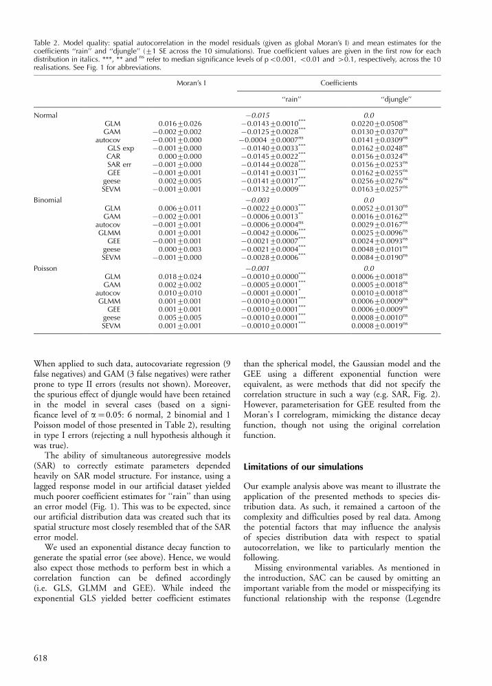
Table 2. Model quality: spatial autocorrelation in the model residuals (given as global Moran’s I) and mean estimates for thecoefficients ‘‘rain’’ and ‘‘djungle’’ (91 SE across the 10 simulations). True coefficient values are given in the first row for eachdistribution in italics. ***, ** and ns refer to median significance levels of pB0.001, B0.01 and "0.1, respectively, across the 10realisations. See Fig. 1 for abbreviations.
Moran’s I Coefficients
‘‘rain’’ ‘‘djungle’’
Normal #0.015 0.0GLM 0.01690.026 #0.014390.0010*** 0.022090.0508ns
GAM #0.00290.002 #0.012590.0028*** 0.013090.0370ns
autocov #0.00190.000 #0.0004 90.0007ns 0.014190.0309ns
GLS exp #0.00190.000 #0.014090.0033*** 0.016290.0248ns
CAR 0.00090.000 #0.014590.0022*** 0.015690.0324ns
SAR err #0.00190.000 #0.014490.0028*** 0.015690.0253ns
GEE #0.00190.001 #0.014190.0031*** 0.016290.0255ns
geese 0.00290.005 #0.014190.0017*** 0.025690.0276ns
SEVM #0.00190.001 #0.013290.0009*** 0.016390.0257ns
Binomial #0.003 0.0GLM 0.00690.011 #0.002290.0003*** 0.005290.0130ns
GAM #0.00290.001 #0.000690.0013** 0.001690.0162ns
autocov #0.00190.001 #0.000690.0004ns 0.002990.0167ns
GLMM 0.00190.001 #0.004290.0006*** 0.002590.0096ns
GEE #0.00190.001 #0.002190.0007*** 0.002490.0093ns
geese 0.00090.003 #0.002190.0004*** 0.004890.0101ns
SEVM #0.00190.000 #0.002890.0006*** 0.008490.0190ns
Poisson #0.001 0.0GLM 0.01890.024 #0.001090.0000*** 0.000690.0018ns
GAM 0.00290.002 #0.000590.0001*** 0.000590.0018ns
autocov 0.01090.010 #0.000190.0001* 0.001090.0018ns
GLMM 0.00190.001 #0.001090.0001*** 0.000690.0009ns
GEE 0.00190.001 #0.001090.0001*** 0.000690.0009ns
geese 0.00590.005 #0.001090.0001*** 0.000890.0010ns
SEVM 0.00190.001 #0.001090.0001*** 0.000890.0019ns
618
1993). This is certainly often a problem in real data,where the ecological determinants of a species’ niche arenot necessarily known and good spatial coverage maynot be available for all the important factors. Also,moderate collinearity among environmental variablesmay lead models to exclude one or more variableswhich would be important in explaining the species’spatial patterning.
Biased spatial error. The autocorrelated error weadded in our simulated data had no bias in geographical(stationarity of the error) or parameter space. Hence ournon-spatial models performed similar to the spatial oneswith regards to parameter estimation, as opposed toremoval of SAC. This may or may not be very differentin real data, where both non-stationarity (Ver Hoefet al. 1993, Brunsdon et al. 1996, Foody 2004,Osborne et al. 2007) and bias in parameter space (e.g.less complete data coverage in warmer regions) can be
found (Lennon 2000, but see Hawkins et al. 2007 foran opposite view).
Mapping bias or mapping heterogeneity can causespatial autocorrelation in real data. If real data resultedfrom several different regional mapping schemes withdifferent protocols or from different people performingthe mapping, data can differ systematically across a gridwith being more similar within a region and moredifferent across.
Spatial autocorrelation at different spatial scales.Several of the methods presented build a ‘‘correctionstructure’’ across all spatial scales (i.e. the variance-covariance matrices in GLS-based models as well asthe spatial eigenvectors), but others do not (theautocovariate and the cluster in geese have one specificspatial scale). Even the former may be dominated bypatterns at one spatial scale, underestimating effects ofanother.
GLM
autocov
CAR
GAM
GEEgeese
GLS expGLS sph GLS gau
SAR errSAR lagSAR mix
SEVM
GLM
autocovGAM
GEEgeese
GLMM expGLMM sph GLMM gau
SEVM-0.02 -0.01 0.00 0.01 0.02 0.03 0.04 0.05-0.012 -0.010 -0.008 -0.006 -0.004 -0.002 0.000
GLM
autocovGAM
GEEgeese
GLMM expGLMM sph GLMM gau
SEVM
estimates for 'rain'
-1.4e-3 -1.2e-3 -1.0e-3 -8.0e-4 -6.0e-4 -4.0e-4 -2.0e-4 0.0
-0.030 -0.025 -0.020 -0.015 -0.010 -0.005 0.000 -0.08 -0.06 -0.04 -0.02 0.00 0.02 0.04 0.06 0.08
estimates for 'djungle'
-0.002 -0.001 0.000 0.001 0.002 0.003
normal
binomial
Poisson
Fig. 1. Comparison of non-spatial (GLM) and spatial modelling approaches for data with normally, binomially and Poisson-distributed errors. Box, whiskers and dots refer to 25/75%, 10/90% and outliers of estimates across 10 realisations of the sameparameter set. Vertical lines indicate true values of parameter. GEE and geese refer to generalised estimating equations with fixedand user-defined correlation structures, respectively. GAM represents a trend-surface regression. GLS and GLMM refer togeneralised least squares-based models with exponential, spherical and Gaussian correlation structure, respectively. SAR(simultaneous autoregressive model) was analysed as error, lag and mixed models. SEVM stands for the spatial eigenvectormapping approach.
619
Finally, small sample sizes make the estimation ofmodel parameters unstable. Adding the additionalparameters for spatial models will further destabilisemodel parameterisation. Also, patterns of SAC in smalldata sets will hinge on very few data points which maydistort the spatial correction.
Discussion
The analysis of species distribution data has reachedhigh statistical sophistication in recent years (Elith et al.2006). However, even the most advanced and compu-ter-intensive statistical procedures are no guarantee forimproving our understanding of the determinants ofspecies distributions, nor of our ability to predictspecies distributions under altered environmental con-ditions (Araujo and Rahbek 2006, Dormann 2007c).One critical step in statistical modelling is the identi-fication of the correct model structure. As pointed outfor experimental ecology in 1984 by Hurlbert, designsanalysed without consideration of the nested nature ofsubsampling are fundamentally flawed. Spatial auto-correlation is a subtle, less obvious form of subsampling(Fortin and Dale 2005): samples from within the rangeof spatial autocorrelation around a data point will addlittle independent information (depending on thestrength of autocorrelation), but unduly inflate samplesize, and thus degrees of freedom of model residuals,thereby influencing statistical inference.
We have presented an overview of different model-ling approaches for the analysis of species distributiondata in which environmental correlates of the distribu-tion are inferred. All these methods can be implementedin freely available software packages (Table 1). Inchoosing between the methods, the type of errordistribution in the response variable will be animportant criterion. For normal data, GLS-basedmethods (GLS, SAR, CAR) can be used efficiently.The most flexible methods, addressing SAC fordifferent error distributions, are spatial GLMMs,GEEs and SEVM. The autocovariate method, too, isflexible, but performed very poorly with regards tocoefficient estimation in our analyses. We encourageusers to try a number of methods, since there is oftennot enough mechanistic information to choose onespecific method a priori. One can use AIC or alike tocompare models (Link and Barker 2006). Note that a‘‘proper’’ (perfectly correctly specified) model wouldnot require the kind of correction the above methodsundertake (Ripley in comments to Besag 1974). In theabsence of a perfect model, however, doing somethingis better than doing nothing (Keitt et al. 2002).
With the exception of autocovariate regression,differences in parameter estimates and inference be-tween spatial and non-spatial models were small for oursimulated data. This was possibly a result of the type ofspatial autocorrelation in, and the simplistic nature of,these data (see section ‘‘Limitations of our simula-tions’’). However, spatial autocorrelation can alsoreflect failure to include an important environmentaldriver in the analysis or inadequate capture of its non-linear effect, so that its spatial autocorrelation cannot beaccounted for by non-spatial models (Besag et al. 1991,
Poisson
distance [no. of cells]0 5 10 15 20
-0.2
0.0
0.2
0.4
0.6
binomial
Mor
an's
I
-0.4
-0.2
0.0
0.2
0.4
0.6
normal
-0.2
0.0
0.2
0.4
0.6
0.8
GLMGAMautocovGLS/GLMM expCARSAR errGEEgeeseSEVM
Fig. 2. Correlograms of one realisation for each of the threedifferent distributions (normal, binomial, Poisson) and themethods compared. See Fig. 1 for abbreviations.
620
Legendre et al. 2002). In either case, spatial autocorre-lation can make a large difference for statistical infe-rence based on spatial data (for review see Dormann,2007a, b, c; for drastic cases of this effect see Tognelliand Kelt 2004 and Kuhn 2007). How to interpretthese differences, especially the shifts in parameterestimates between spatial and non-spatial modelscommonly observed in real data, remains controversial.While Lennon (2000) and others (Tognelli andKelt 2004, Jetz et al. 2005, Dormann 2007b, Kuhn2007) argue that spatial autocorrelation in species
distribution models may well bias coefficient estima-tion, Diniz-Filho et al. (2003) and Hawkins et al.(2007) found non-spatial model to be robust andunbiased for several data sets. So far, no extensivesimulation study has been carried out to investigate howspatial versus non-spatial methods perform underdifferent forms and causes of SAC. Implementing alagged autocorrelation structure to simplistic data didnot reveal a bias in parameter estimation in OLS(Kissling and Carl 2007), consistent with the results ofHawkins et al. (2007).
Fig. 3. The two environmental covariates, raw distributional data and residual maps for the different methods for one realisationof the data with normally distributed errors. Blue indicates positive, red negative values. Quadrat size is proportional to the valueof the residual (or raw data value), but scaling is different for every plot (since a comparison of quadrat sizes would simply be acomparison of model fit). See Fig. 1 for abbreviations.
621
One of the two most striking findings of ouranalyses is the high error rate of the autocovariatemethod. Most methods for normally distributed datayielded coefficient estimates for ‘‘rain’’ that wereacceptable, including the non-spatial ordinary leastsquare regression (Fig. 1). However, two modelsperformed poorly: both the autocovariate regressionand the lag version of the simultaneous autoregressivemodel showed a very consistent and strong bias, leadingto severe underestimation (in absolute terms) of modelcoefficients. A similar pattern was also found for thenon-normally distributed errors, identifying autocovari-ate regression as a consistently worse performer than theother approaches. The poor performance of the auto-covariate regression approach in our study with regardsto parameter estimation contrasts with earlier evalua-tions of this method (Augustin et al. 1996, Huffer andWu 1998, Hoeting et al. 2000, He et al. 2003), but isin line with more recent ones (Dormann 2007a, Carland Kuhn 2007a). These earlier studies used moresophisticated parameter estimation techniques, suggest-ing that the inferiority of autocovariate models in oursimulation may partly result from our simplistic (butnot unusual) implementation of the method. Moreover,two of the earlier studies were undertaken in the contextof many missing values: Augustin et al. (1996) usedonly 20% of sites in their study area for model training;Hoeting et al. (2000) used between 3.8 and 5.8%. Thismay have diminished the influence of any autocovariateand perhaps explains why in these studies the auto-covariate did not overwhelm other model coefficients(as it did in ours). A final reason for the discrepancy infindings may be that our artificial data simulated spatialautocorrelation in the error structure, whereas othersimulations created spatial structure directly in theresponse values, which more closely reflects the assump-tions underlying autocovariate models.
The second interesting finding is the overall highervariability of results for binary data. While for normal-and Poisson-distributed residuals all model approaches(apart from autocovariate regression) yielded similarresults and little variance across the ten realisations(Fig. 1), a different pattern emerged for binary(binomial) data. We attribute this to the relatively lowinformation content of binary data (Breslow andClayton 1993, Venables and Ripley 2002), makingparameterisation of the model very dependent on thosedata points that determine the point of inflexion of thelogistic curve (McCullough and Nelder 1989). Thisphenomenon has been noted before (McCullough andNelder 1989), and remains relevant for species dis-tribution models, where the majority of studies arebased on the analysis of presence-absence data (Guisanand Zimmermann 2000, Guisan and Thuiller 2005).
Tricks and tips
Each of the above methods has its quirks and somerequire fine-tuning by the analyst. Without attemptingto cover these comprehensively, we here hint at someareas for each method type which require attention.
In autocovariate regression, neighbourhood size andtype of weighting function are potentially sensitiveparameters, which can be optimised through trial anderror. It seems, however, that small neighbourhood sizes(such as the next one to two cells) often turn out best,and that the type of weighting function has relativelylittle effect. This was the case in our analysis as well as inpublished studies investigating different neighbourhoodsizes (for review see Dormann 2007b). Anotherimportant aspect of autocovariate models is theapproach chosen to dealing with missing data, whichmay lead to cells without neighbours (‘‘islands’’). Sincethe issue arises for all modelling methods, we shallbriefly discuss it here. Missing data can be overcome bya) omission (Klute et al. 2002, Moore and Swihart2005); b) strategic choice of neighbourhood structure(Smith 1994); c) estimating missing response values byinitially ignoring spatial autocorrelation and regressingknown response values against explanatory variablesother than the autocovariate (Augustin et al. 1996,Teterukovskiy and Edenius 2003, Segurado and Araujo2004); and d) as in c), but then refining it throughan iterative procedure known as the Gibbs sampler(Casella and George 1992). This procedure is compu-tationally intensive, but has been found to yield the bestresults (Augustin et al. 1996, Wu and Huffer 1997,Osborne et al. 2001, Teterukovskiy and Edenius 2003,Brownstein et al. 2003, He et al. 2003). Simulationstudies further suggest that a) parameter estimation ispoor when the autocovariate effect is strong relative tothe effect of other explanatory variables (Wu andHuffer 1997, Huffer and Wu 1998); b) the precisionof parameter estimates varies with species prevalence,i.e. the number of presence records relative to the totalsample size (Hoeting et al. 2000); and c) autocovariatemodels adequately distinguish between meaningfulexplanatory variables and random covariates (Hoetinget al. 2000) (but not in our study). Both simulation andempirical studies also indicate that autocovariate modelsachieve better fit than equivalent models lacking theautocovariate term (Augustin et al. 1996, Hoeting et al.2000, Osborne et al. 2001, He et al. 2003, McPhersonand Jetz 2007).
For spatial eigenvector mapping, computationalspeed becomes an issue for large datasets. Althoughthe calculation of eigenvectors itself is rapid, optimisingthe model by permutation-based testing combinationsof spatial eigenvectors is computer-intensive. Diniz-Filho and Bini (2005) argue that the identity of theselected eigenvectors is indicative of the spatial scales at
622
which spatial autocorrelation takes effect, making thismethod potentially very interesting for ecologists. Theimplementation used in our analysis requires littlearbitration and hence should be explored more widely.Note that SEVM, in the way that was applied here, isbased on a different modelling philosophy. Its declaredaim is to remove residual spatial autocorrelation, unlikeall other methods described above, which simplyprovide a mathematical way to incorporate SAC intothe analysis.
For the GLS-based methods (GLS and the spatialGLMM), estimation of the correlation structure func-tions (i.e. the parameter r) can be rather unstable. As aconsequence some models yield r"0 (i.e. no spatialautocorrelation incorporated) or r:#, with the GLSmodel returning what is in fact a non-spatial GLM ornonsensical results, respectively. This problem can beovercome by inclusion of a ‘‘nugget’’ term that reducesthe correlation at infinitesimally small distances to avalue below 1, or, even better, a specification of r basedon a semi-variogram of the residuals (Littell et al. 1996,Kaluzny et al. 1998). The common justification for anugget term are measurement errors (on top of thespatially correlated error); including a nugget effect canstabilize the estimation of the correlation function(Venables and Ripley 2002).
Autoregressive models (SAR and CAR) require adecision on the weighting scheme for the weightsmatrix, for which there is not always an a priori reason.The main options are row standardised coding (sumsover all rows add up to N), globally standardised coding(sums over all links add up to N), dividing globallystandardised neighbours by their number (sums over alllinks add up to unity), or the variance-stabilising codingscheme proposed by Tiefelsdorf et al. (1999, pp. 167!168), i.e. sums over all links to N. In our analysis, therow standardised coding was most often the superiorchoice, which is in line with other studies (Kissling andCarl 2007), but the binary and the variance-stabilisingcoding scheme also resulted in good models. SAR andCAR models did not differ much in our analysis.According to Cressie (1993), CAR models should bepreferred in terms of estimation and interpretation,although SAR models are preferred in the econo-metric context (Anselin 1988). Either approachcan be relatively slow for large data sets (samplesize"10 000) due to the estimation of the determinantof (I!rW) for each step of the iteration. Note thatBayesian CAR models do not require the computationof such a determinant and can therefore be particularlysuitable for data on large lattices (Gelfand andVounatsou 2003). For SAR models, identification ofthe correct model structure is recommended and modelselection procedures can help to reduce bias (Kisslingand Carl 2007). The Lagrange-test (Appendix) canalso help here. However, SAR error models generally
perform better than SAR lag or even SAR mix modelswhen tackling simulated data containing autocorrela-tion in lagged predictors (or response and predictors), asrecently demonstrated in a more comprehensive assess-ment of SAR models using different spatially auto-correlated datasets (Kissling and Carl 2007).
Generalised estimating equations require high sto-rage capacity for solving the GEE score equationwithout clustering as we used it in our fixed model.Application of the fixed model will therefore be limitedfor models on data with larger sample size, but themethod is very suitable for missing data and non-latticedata. The need in storage capacity is considerablyreduced by cluster models, such as our user-definedmodel. But clustering requires attention to three stepsin the analysis: cluster size, within-cluster correlationstructure and allocation of cells to clusters. To find thebest cluster size for the analysis, we recommendinvestigating clusters of 2%2, 3%3 and 4%4. In realdata, these cluster sizes have been sufficient to removespatial autocorrelation (Carl and Kuhn 2007a). Severaldifferent correlation structures should be computedinitially, e.g. to allow for anisotropy. Finally, allocationof cells to clusters can start in different places.Depending on the starting point (e.g. top right ornorth west), cells will be placed in different clusters.Choosing different starting points will give the analystan idea of the (in our experience limited) importance ofthis issue. Computing time is short.
Autocorrelation in a predictive setting
Spatial autocorrelation may arise for a number ofecological reasons, including external environmentaland historical factors limiting the mobility of organ-isms, intrinsic organism-specific dispersal mechanismsand other behavioural factors causing the spatialaggregation of populations and species in the land-scapes. In addition to these factors, spatial autocorrela-tion can also be caused by observer bias and differencesin sampling schemes and sampling effort. Overall,spatial autocorrelation occurs at all spatial scales fromthe micrometre to hundreds of kilometres (Dormann2007b), possibly for a whole suite of reasons. Sincethese reasons are mostly unknown, one cannot readilyderive a spatial correlation structure for an entirely new,unobserved region. Augustin et al. (1996) and others(Hoeting et al. 2000, Teterukovskiy and Edenius 2003,Reich et al. 2004) have, however, successfully used theGibbs sampler (Casella and George 1992) to derivepredictions for unobserved areas within the study region(interpolation), and He et al. (2003) extrapolatedautologistic predictions through time to examinepossible effects of climate change.
623
Interpolation, i.e. the prediction of values within theparameter and spatial range, can be achieved by severalof the presented methods. An advantage of GLS is thatthe spatially correlated error can be predicted for siteswhere no observations are available, based on the valuesof observed sites (e.g. kriging). The same holds true forthe spatial GLMM. For autocovariate regression andspatial eigenvector mapping, in contrast, interpolationis more complicated, requiring use of the aforemen-tioned Gibbs-sampler.
When models are projected into new geographicareas or time periods the handling of spatial auto-correlation becomes more problematic (if not impos-sible). Extrapolation in time, for example, is necessarilyuncertain, particularly if biotic interactions ! and withthem spatial autocorrelation patterns ! could change aseach species responds differentially to climate change.However; most of the statistical methods used forprediction in time neglect important processes such asmigration, dispersal, competition, predation (Pearsonand Dawson 2003, Dormann 2007c), or at least assumemany of them to remain constant. One might thereforeargue that, while taking the autocorrelation structure asconstant adds one more assumption, the use of spatialparameters at least helps to derive better models.Extrapolation in space, in contrast, is not recom-mended: the variance-covariance matrix parameterisedin GLS approaches, for example, may look verydifferent in other regions, even for the same organism.Hence, extrapolation can only be based on thecoefficient estimates, not on the spatial component ofthe model. Extrapolation is further complicated bymodel complexity. The use of non-linear predictors andinteractions between environmental variables will in-crease model fit, but compromises transferability ofmodels in time and space (Beerling et al. 1995, Sykes2001, Gavin and Hu 2006). Our study therefore didnot compare methods’ abilities to either make predic-tions to new geographic areas or extrapolate beyond therange of environmental parameters.
Bayesian approaches
Our review focused on frequentist methods. Bayesianmethods, which allow prior beliefs about data to beincorporated in the calculation of expected values, offeran alternative. Experience and a good understanding ofthe influence of prior distributions and convergenceassessment of Markov chains are crucial in Bayesiananalyses. Thus, if therefore the question of interest canbe addressed using more robust, less computationallyintensive methods, there is no real need to applythe ‘‘Bayesian machinery’’ (Brooks 2003). The spatialanalyses as presented in this paper can bedone straightforwardly using non-Bayesian methods.
However, Bayesian methods for the analyses of speciesdistribution data are more flexible; they can be moreeasily extended to include more complex structures(Latimer et al. 2006). Models can for example beextended to a multivariate setting when several (corre-lated) counts of different species in each grid cell are tobe modelled, or when both count and normallydistributed data are to be modelled within the sameframework (Thogmartin et al. 2004, Kuhn et al. 2006).Bayesian methods are also a generally more suitable toolfor inference in data sets with many missing values, orwhen accounting for detection probabilities (Gelfandet al. 2005, Kuhn et al. 2006).
Wishlist
In this study, we introduced a wide range of statisticaltools to deal with spatial autocorrelation in speciesdistribution data. Unfortunately, none of these toolsdirectly represents dynamic aspects of ecological reality(e.g. dispersal, species interaction): all the methodsexamined remain phenomenological rather than me-chanistic. Therefore they are unable to disentanglestochastic and process-introduced spatial autocorrela-tion. Disentangling these sources of spatial autocorrela-tion in the data would be particularly important for theanalysis of species that are not at equilibrium with theirenvironmental drivers (e.g. newly introduced speciesexpanding in range or species that have undergonepopulation declines due to overexploitation). Moreover,it would be desirable to extend the statistical approachesused here to model multivariate response variables, suchas species composition (see Kuhn et al. 2006, for anexample). Similarly, presence-only data, as commonlyfound for museum specimens, cannot be analysed withthe above methods, nor are we aware of any methodsuitable for such data. While in principle it is possibleto incorporate temporal and/or phylogenetic compo-nents into species distribution models (e.g. into GEEs,GLMMs and Bayes), this has not yet been attempted. Italso would be desirable to have methods available thatallow for the strengths of spatial autocorrelation to varyin space (non-stationarity), since stationarity is a basicand strong assumption of all the methods used here(except perhaps SEVM). Finally, the issue of variableselection under spatial autocorrelation has receivedvirtually no coverage in the statistical literature, andhence the effect of spatial autocorrelation on theidentification of the best-fitting model, or candidateset of most likely models, still remains unclear.
Authors’ contributions and acknowledgements ! Data werecreated by CFD, GC and FS. Analyses and manuscriptsections describing each method were carried out as follows:autocovariate regression: JMM; SEVM: PRPN and RB;
624
GAM: JB, RO and CFD; GLS: BR and WJ; CAR: BS; SAR:WDK; GLMM: FMS and RGD; GEE: GC and IK. Furtheranalyses, figure and table preparation and initial drafting werecarried out by CFD. All authors contributed to writing thefinal manuscript.
We also would like to thank Pierre Legendre, CarstenRahbek, Alexandre Diniz-Filho, Jack Lennon and ThiagoRangel for comments on an earlier version. This contributionis based on the international workshop ‘‘Analysing SpatialDistribution Data: Principles, Applications and Software’’(GZ 4850/191/05) funded by the German Science Founda-tion (DFG), awarded to CFD. CFD acknowledges funding bythe Helmholtz Association (VH-NG-247). JMM’s work issupported by the Lenfest Ocean Program. MBA, GC, IK, RO& BR acknowledge funding by the European Union withinthe FP 6 Integrated Project ‘‘ALARM’’ (GOCE-CT-2003-506675). GC acknowledges a stipend from the federal state‘‘Sachsen-Anhalt’’, Ministry of Education and CulturalAffairs. WDK & IK acknowledge support from the ‘‘VirtualInst. for Macroecology’’, funded by the Helmholtz Associa-tion (VH-VI-153 Macroecology). RGD was supported byNERC (grant no. NER/O/S/2001/01257). PEPN researchwas supported by NSERC.
References
Albert, P. S. and McShane, L. M. 1995. A generalizedestimating equations approach for spatially correlatedbinary data: with an application to the analysis ofneuroimaging data. ! Biometrics 51: 627!638.
Anon. 2005. R: a language and environment for statisticalcomputing. ! R Foundation for Statistical Computing.
Anselin, L. 1988. Spatial econometrics: methods and models.! Kluwer.
Anselin, L. 2002. Under the hood: issues in the specificationand interpretation of spatial regression models. ! Agricult.Econ. 17: 247!267.
Araujo, M. B. and Williams, P. H. 2000. Selecting areas forspecies persistence using occurrence data. ! Biol. Conserv.96: 331!345.
Araujo, M. B. and Rahbek, C. 2006. How does climatechange affect biodiversity? ! Science 313: 1396!1397.
Augustin, N. H. et al. 1996. An autologistic model for thespatial distribution of wildlife. ! J. Appl. Ecol. 33: 339!347.
Augustin, N. H. et al. 1998. The role of simulation inmodelling spatially correlated data. ! Environmetrics 9:175!196.
Augustin, N. H. et al. 2005. Analyzing the spread of beechcanker. ! For. Sci. 51: 438!448.
Bai, Z. et al. 1996. Some large-scale matrix computationproblems. ! J. Comput. Appl. Math. 74: 71!89.
Beerling, D. J. et al. 1995. Climate and the distribution ofFallopia japonica!use of an introduced species to test thepredictive capacity of response surfaces. ! J. Veg. Sci. 6:269!282.
Besag, J. 1974. Spatial interaction and the statistical analysisof lattice systems. ! J. Roy. Stat. Soc. B 36: 192!236.
Besag, J. et al. 1991. Bayesian image restoration with twoapplications in spatial statistics (with discussion). ! Ann.Inst. Stat. Math. 43: 1!59.
Bivand, R. 2005. spdep: spatial dependence: weightingschemes, statistics and models. ! R package version 0.3!17.
Bjørnstad, O. N. and Falck, W. 2000. Nonparametric spatialcovariance functions: estimation and testing. ! Environ.Ecol. Stat. 8: 53!70.
Borcard, D. and Legendre, P. 2002. All-scale spatial analysisof ecological data by means of principal coordinates ofneighbour matrices. ! Ecol. Modell. 153: 51!68.
Breslow, N. E. and Clayton, D. G. 1993. Approximateinference in generalized linear mixed models. ! J. Am.Stat. Assoc. 88: 9!25.
Brooks, S. P. 2003. Bayesian computation: a statisticalrevolution. ! Phil. Trans. R. Soc. A 361: 2681!2697.
Brownstein, J. S. et al. 2003. A climate-based model predictsthe spatial distribution of the Lyme disease vector Ixodesscapularis in the United States. ! Environ. Health Persp.111: 1152!1157.
Brunsdon, C. et al. 1996. Geographically weighted regression:a method for exploring spatial non-stationarity. ! Geogr.Analys. 28: 281!298.
Carey, V. J. 2002. gee: generalized estimation equation solver.Ported to R by Thomas Lumley (ver. 3.13, 4.4) and BrianRipley. ! Bwww.r-project.org".
Carl, G. and Kuhn, I. 2007a. Analyzing spatial autocorrela-tion in species distributions using Gaussian and logitmodels. ! Ecol. Modell. 207: 159!170.
Carl, G. and Kuhn, I. 2007b. Analyzing spatial ecological datausing linear regression and wavelet analysis. ! Stochast.Environ. Res. Risk Assess., in press.
Casella, G. and George, E. I. 1992. Explaining the Gibbssampler. ! Am. Stat. 46: 167!176.
Cliff, A. D. and Ord, J. K. 1981. Spatial processes: modelsand applications. ! Pion.
Clifford, P. et al. 1989. Assessing the significance of thecorrelation between two spatial processes. ! Biometrics 45:123!134.
Cressie, N. A. C. 1993. Statistics for spatial data. ! Wiley.Dark, S. J. 2004. The biogeography of invasive alien plants in
California: an application of GIS and spatial regressionanalysis. ! Div. Distrib. 10: 1!9.
Davies, R. G. et al. 2006. Human impacts and the globaldistribution of extinction risk. ! Proc. R. Soc. B 273:2127!2133.
Diggle, P. J. et al. 1995. Analysis of longitudinal data.! Clarendon.
Diniz-Filho, J. A. and Bini, L. M. 2005. Modellinggeographical patterns in species richness using eigenvec-tor-based spatial filters. ! Global Ecol. Biogeogr. 14: 177!185.
Diniz-Filho, J. A. F. et al. 1998. An eigenvector method forestimating phylogenetic inertia. ! Evolution 52: 1247!1262.
Diniz-Filho, J. A. F. et al. 2003. Spatial autocorrelation andred herrings in geographical ecology. ! Global Ecol.Biogeogr. 12: 53!64.
Dobson, A. J. 2002. An introduction to generalized linearmodels. ! Chapman and Hall.
625
Dormann, C. F. 2007a. Assessing the validity of autologisticregression. ! Ecol. Modell. 207: 234!242.
Dormann, C. F. 2007b. Effects of incorporating spatialautocorrelation into the analysis of species distributiondata. ! Global Ecol. Biogeogr. 16: 129!138.
Dormann, C. F. 2007c. Promising the future? Global changepredictions of species distributions. ! Basic Appl. Ecol.8: 387!397.
Dray, S. et al. 2006. Spatial modeling: a comprehensiveframework for principal coordinate analysis of neighbormatrices (PCNM). ! Ecol. Modell. 196: 483!493.
Dutilleul, P. 1993. Modifying the t test for assessing thecorrelation between two spatial processes. ! Biometrics 49:305!314.
Elith, J. et al. 2006. Novel methods improve prediction ofspecies’ distributions from occurrence data. ! Ecography29: 129!151.
Ferrier, S. et al. 2002. Extended statistical approaches tomodelling spatial pattern in biodiversity in northeast NewSouth Wales. I. Species-level modelling. ! Biodiv. Con-serv. 11: 2275!2307.
Foody, G. M. 2004. Spatial nonstationarity and scale-dependency in the relationship between species richnessand environmental determinants for the sub-Saharanendemic avifauna. ! Global Ecol. Biogeogr. 13: 315!320.
Fortin, M. J. and Dale, M. R. T. 2005. Spatial analysis ! aguide for ecologists. ! Cambridge Univ. Press.
Fotheringham, A. S. et al. 2002. Geographically weightedregression: the analysis of spatially varying relationships.! Wiley.
Gavin, D. G. and Hu, F. S. 2006. Spatial variation of climaticand non-climatic controls on species distribution: therange limit of Tsuga heterophylla. ! J. Biogeogr. 33: 1384!1396.
Gelfand, A. E. and Vounatsou, P. 2003. Proper multivariateconditional autoregressive models for spatial data analysis.! Biostatistics 4: 11!25.
Gelfand, A. E. et al. 2005. Modelling species diversitythrough species level hierarchical modelling. ! Appl.Stat. 54: 1!20.
Griffith, D. A. 2000a. Eigenfunction properties and approx-imations of selected incidence matrices employed inspatial analyses. ! Lin. Algebra Appl. 321: 95!112.
Griffith, D. A. 2000b. A linear regression solution to thespatial autocorrelation problem. ! J. Geogr. Syst. 2: 141!156.
Griffith, D. A. and Peres-Neto, P. R. 2006. Spatial modelingin ecology: the flexibility of eigenfunction spatial analysesin exploiting relative location information. ! Ecology 87:2603!2613.
Guisan, A. and Zimmermann, N. E. 2000. Predictive habitatdistribution models in ecology. ! Ecol. Modell. 135: 147!186.
Guisan, A. and Thuiller, W. 2005. Predicting speciesdistributions: offering more than simple habitat models.! Ecol. Lett. 8: 993!1009.
Gumpertz, M. L. et al. 1997. Autologistic model of spatialpattern of Phytophthora epidemic in bell pepper: effects ofsoil variables on disease presence. ! J. Agricult. Biol.Environ. Stat. 2: 131!156.
Haining, R. 2003. Spatial data analysis ! theory and practice.! Cambridge Univ. Press.
Hastie, T. J. and Tibshirani, R. J. 1990. Generalized additivemodels. ! Chapman and Hall.
Hawkins, B. A. et al. 2007. Red herrings revisited: spatialautocorrelation and parameter estimation in geographicalecology. ! Ecography 30: 375!384.
He, F. L. et al. 2003. Autologistic regression model for thedistribution of vegetation. ! J. Agricult. Biol. Environ.Stat. 8: 205!222.
Hoeting, J. A. et al. 2000. An improved model for spatiallycorrelated binary responses. ! J. Agricult. Biol. Environ.Stat. 5: 102!114.
Hooten, M. B. et al. 2003. Predicting the spatial distributionof ground flora on large domains using a hierarchicalBayesian model. ! Landscape Ecol. 18: 487!502.
Huffer, F. W. and Wu, H. L. 1998. Markov chain MonteCarlo for autologistic regression models with applicationto the distribution of plant species. ! Biometrics 54: 509!524.
Hurlbert, S. H. 1984. Pseudoreplication and the design ofecological experiments. ! Ecol. Monogr. 54: 187!211.
Isaaks, E. H. and Shrivastava, R. M. 1989. An introduction toapplied geostatistics. ! Oxford Univ. Press.
Jetz, W. and Rahbek, C. 2002. Geographic range size anddeterminants of avian species richness. ! Science 297:1548!1551.
Jetz, W. et al. 2005. Local and global approaches to spatialdata analysis in ecology. ! Global Ecol. Biogeogr. 17: 97!98.
Kaboli, M. et al. 2006. Avifaunal gradients in two arid zonesof central Iran in relation to vegetation, climate, andtopography. ! J. Biogeogr. 33: 133!144.
Kaluzny, S. P. et al. 1998. S-plus spatial stats user’s manualfor Windows and Unix. ! Springer.
Keitt, T. H. et al. 2002. Accounting for spatial pattern whenmodeling organism-environment interactions. ! Ecogra-phy 25: 616!625.
Kissling, W. D. and Carl, G. 2007. Spatial autocorrelationand the selection of simultaneous autoregressive models. !Global Ecol. Biogeogr., in press.
Klute, D. S. et al. 2002. Autologistic regression modeling ofAmerican woodcock habitat use with spatially dependentdata. ! In: Scott, J. M. et al. (eds), Predicting speciesoccurrences: issues of accuracy and scale. Island Press, pp.335!343.
Knapp, R. A. et al. 2003. Developing probabilistic models topredict amphibian site occupancy in a patchy landscape.! Ecol. Appl. 13: 1069!1082.
Kupfer, J. A. and Farris, C. A. 2007. Incorporating spatialnon-stationarity of regression coefficients into predictivevegetation models. ! Landscape Ecol. 22: 837!852.
Kuhn, I. 2007. Incorporating spatial autocorrelation mayinvert observed patterns. ! Div. Distrib. 13: 66!69.
Kuhn, I. et al. 2006. Relating geographical variation inpollination types to environmental and spatial factorsusing novel statistical methods. ! New Phytol. 72: 127!139.
Latimer, A. M. et al. 2006. Building statistical models toanalyze species distributions. ! Ecol. Appl. 16: 33!50.
626
Legendre, P. 1993. Spatial autocorrelation: trouble or newparadigm? ! Ecology 74: 1659!1673.
Legendre, P. and Fortin, M.-J. 1989. Spatial pattern andecological analysis. ! Vegetatio 80: 107!138.
Legendre, P. and Legendre, L. 1998. Numerical ecology.! Elsevier.
Legendre, P. et al. 2002. The consequences of spatial structurefor the design and analysis of ecological field surveys.! Ecography 25: 601!615.
Lennon, J. J. 2000. Red-shifts and red herrings in geographi-cal ecology. ! Ecography 23: 101!113.
Liang, K. Y. and Zeger, S. L. 1986. Longitudinal data analysisusing generalized linear models. ! Biometrika 73: 13!22.
Lichstein, J. W. et al. 2002. Spatial autocorrelation andautoregressive models in ecology. ! Ecol. Monogr. 72:445!463.
Liebhold, A. M. and Gurevitch, J. 2002. Integrating thestatistical analysis of spatial data in ecology. ! Ecography25: 553!557.
Link, W. A. and Barker, R. J. 2006. Model weights and thefoundations of multimodel inference. ! Ecology 87:2626!2635.
Littell, R. C. et al. 1996. SAS system for mixed models.! SAS Publ.
Luoto, M. et al. 2001. Determinants of distribution andabundance in the clouded apollo butterfly: a landscapeecological approach. ! Ecography 24: 601!617.
McCullough, P. and Nelder, J. A. 1989. Generalized linearmodels. ! Chapman and Hall.
McPherson, J. M. and Jetz, W. 2007. Effects of species’ecology on the accuracy of distribution models.! Ecography 30: 135!151.
Miller, J. et al. 2007. Incorporating spatial dependence inpredictive vegetation models. ! Ecol. Modell. 202: 225!242.
Moore, J. E. and Swihart, R. K. 2005. Modeling patchoccupancy by forest rodents: incorporating detectabilityand spatial autocorrelation with hierarchically structureddata. ! J. Wildl. Manage. 69: 933!949.
Myers, R. H. et al. 2002. Generalized linear models. ! Wiley.Orme, C. D. L. et al. 2005. Global hotspots of species
richness are not congruent with endemism or threat.! Nature 436: 1016!1019.
Osborne, P. E. et al. 2001. Modelling landscape-scale habitatuse using GIS and remote sensing: a case study with greatbustards. ! J. Appl. Ecol. 38: 458!471.
Osborne, P. E. et al. 2007. Non-stationarity and localapproaches to modelling the distributions of wildlife.! Div. Distribut., in press.
Palma, L. et al. 1999. The use of sighting data to analyseIberian lynx habitat and distribution. ! J. Appl. Ecol. 36:812!824.
Pearson, R. G. and Dawson, T. P. 2003. Predicting theimpacts of climate change on the distribution of species:are bioclimate envelope models useful? ! Global Ecol.Biogeogr. 12: 361!371.
Perry, J. N. et al. 2002. Illustrations and guidelines forselecting statistical methods for quantifying spatial pa-terrns in ecological data. ! Ecography 25: 578!600.
Pinheiro, J. C. and Bates, D. M. 2000. Mixed-effect modelsin S and S-plus. ! Springer.
Rangel, T. F. L. V. B. et al. 2006. Towards an integratedcomputational tool for spatial analysis in macroecologyand biogeography. ! Global Ecol. Biogeogr. 15: 321!327.
Reich, R. M. et al. 2004. Predicting the location of northerngoshawk nests: modeling the spatial dependency betweennest locations and forest structure. ! Ecol. Modell. 176:109!133.
Segurado, P. and Araujo, M. B. 2004. An evaluation ofmethods for modelling species distributions. ! J. Bio-geogr. 31: 1555!1568.
Segurado, P. et al. 2006. Consequences of spatial autocorrela-tion for niche-based models. ! J. Appl. Ecol. 43: 433!444.
Smith, P. A. 1994. Autocorrelation in logistic regressionmodelling of species’ distributions. ! Global. Ecol.Biogeogr. Lett. 4: 47!61.
Sokal, R. R. and Oden, N. L. 1978a. Spatial autocorrelationin biology. I. Methodology. ! Biol. J. Linn. Soc. 10:199!228.
Sokal, R. R. and Oden, N. L. 1978b. Spatial autocorrelationin biology. II. Some biological implications and fourapplications of evolutionary and ecological interest.! Biol. J. Linn. Soc. 10: 229!249.
Stephenson, C. M. et al. 2006. Modelling establishmentprobabilities of an exotic plant, Rhododendron ponticum,invading a heterogeneous, woodland landscape usinglogistic regression with spatial autocorrelation. ! Ecol.Modell 193: 747!758.
Sykes, M. T. 2001. Modelling the potential distribution andcommunity dynamics of lodgepole pine (Pinus contortaDougl. ex. Loud.) in Scandinavia. ! For. Ecol. Manage.141: 69!84.
Teterukovskiy, A. and Edenius, L. 2003. Effective fieldsampling for predicting the spatial distribution of reindeer(Rangifer tarandus) with help of the Gibbs sampler.! Ambio 32: 568!572.
Thogmartin, W. E. et al. 2004. A hierarchical spatial model ofavian abundance with application to Cerulean warblers.! Ecol. Appl. 14: 1766!1779.
Tiefelsdorf, M. et al. 1999. A variance-stabilizing codingscheme for spatial link matrices. ! Environ. Plann. A 31:165!180.
Tobler, W. R. 1970. A computer movie simulating urbangrowth in the Detroit region. ! Econ. Geogr. 46: 234!240.
Tognelli, M. F. and Kelt, D. A. 2004. Analysis of determi-nants of mammalian species richness in South Americausing spatial autoregressive models. ! Ecography 27: 427!436.
Venables, W. N. and Ripley, B. D. 2002. Modern appliedstatistics with S. ! Springer.
Ver Hoef, J. M. et al. 1993. Spatial models for spatialstatistics: some unification. ! J. Veg. Sci. 4: 441!452.
Wall, M. M. 2004. A close look at the spatial structureimplied by the CAR and SAR models. ! J. Stat. Plann.Infer. 121: 311!324.
Waller, L. A. and Gotway, C. A. 2004. Applied spatialstatistics for public health data. ! Wiley.
Wood, S. N. 2006. Generalized additive models. ! Chapmanand Hall/CRC.
627
Worm, B. et al. 2005. Global patterns of predator diversity inthe open oceans. ! Science 309: 1365!1369.
Wu, H. L. and Huffer, F. W. 1997. Modelling thedistribution of plant species using the autologistic regres-sion model. ! Environ. Ecol. Stat. 4: 49!64.
Yamaguchi, N. et al. 2003. Habitat preferences of feralAmerican mink in the Upper Thames. ! J. Mammal. 84:1356!1373.
Yan, J. 2002. geepack: yet another package for generalizedestimating equations. ! R News 2: 12!14.
Yan, J. 2004. geepack: generalized estimating equationpackage. ! R package version 0.2!10.
Download the appendix as file E5171 fromBwww.oikos.ekol.lu.se/appendix".
628