mechanical behavior of polyurea … · scientifiques de niveau recherche, ... mechanical behavior...

HAL Id: dumas-00578094https://dumas.ccsd.cnrs.fr/dumas-00578094

Submitted on 18 Mar 2011

HAL is a multi-disciplinary open accessarchive for the deposit and dissemination of sci-entific research documents, whether they are pub-lished or not. The documents may come fromteaching and research institutions in France orabroad, or from public or private research centers.

L’archive ouverte pluridisciplinaire HAL, estdestinée au dépôt et à la diffusion de documentsscientifiques de niveau recherche, publiés ou non,émanant des établissements d’enseignement et derecherche français ou étrangers, des laboratoirespublics ou privés.

Mechanical behavior of polyurea nanocomposites dopedwith nanoparticles

Emilien Billaudeau

To cite this version:Emilien Billaudeau. Mechanical behavior of polyurea nanocomposites doped with nanoparticles. Ma-terials. 2010. <dumas-00578094>

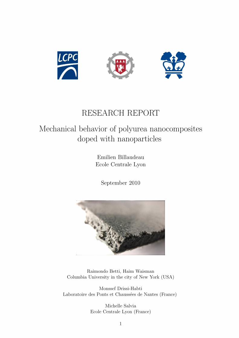
https://dumas.ccsd.cnrs.fr/dumas-00578094

https://hal.archives-ouvertes.fr

RESEARCH REPORT

Mechanical behavior of polyurea nanocompositesdoped with nanoparticles

Emilien BillaudeauEcole Centrale Lyon

September 2010

Raimondo Betti, Haim WaismanColumbia University in the city of New York (USA)

Monssef Drissi-HabtiLaboratoire des Ponts et Chaussees de Nantes (France)

Michelle SalviaEcole Centrale Lyon (France)

1

Blank page

Research report 2 Emilien Billaudeau

Acknowledgments

My most earnest acknowledgment must go to my advisors from Columbia Univer-sity1, professors Betti and Waisman who have been instrumental in ensuring myintegration in the Civil Engineering department. I also thank them to have givenme scientific and financial support to perform my study.

My internship would not have been possible without the matchless help I gotfrom Dr. Monssef Drissi-Habti from the LCPC2 who connected me with this labo-ratory and helped me in my research. This training period is conducted within theframework of the collaboration going on between LCPC and Columbia University.

My gratitude also stretches to my second French advisor, Pr. Michelle Salviafrom the ECL3. Her experience in material science and particularly in compositeswas really helpful.

Mr. Adrian Brugger and Dr. Liming Li from the Carleton laboratory (Depart-ment of Civil Engineering at Columbia University) are greatly acknowledged fortheir assistance with the material manufacturing and the tension tests.

I would also like to thank Oya Okman for her help with the Scanning ElectronMicroscope and for her training session in order to give me access.

Last but not least, i would like to express my gratitude to Dr. Jorgen Bergstrom4

for his extra support he gave me on the computational modeling.

1(New York, USA)

2Laboratoire Central des Ponts et Chaussees (Nantes, France)

3Ecole Centrale (Lyon, France)

4MIT Ph.D., Veryst Engineering (Boston, USA)


Abstract

Recently, carbon nanotubes and graphene nanoplatelets have attracted both aca-demic and industrial interest because of their capacity to produce a dramatic im-provement in properties at very low filler content. In this work, we focused onexperimental studies and computational modeling of polymer nanocomposites in-tended for passive protection of civil structures. The material considered in thisstudy consisted of a polyurea matrix enhanced by different quantities of nanopar-ticles. Different renforts and matrixes have been used to fabricate nanoparticlespolymer nanocomposites by a range of methods. Several tensile tests were per-formed to evaluate and characterize the behavior of the studied materials in orderto choose the appropriate manufacturing protocol and the suitable enhancement.Furthermore, a finite elements model was achieved The main goal of this study wasto achieve a parametric determination of the tested materials in order to find a gen-eral model.

The manufacturing protocol study had led to an ultrasonic dispersion of thenanoparticles instead of a mechanical stirring. Degrading the properties of the ini-tial material, the mechanical mixing method does not disaggregate the nanoparticles,which is an important factor in the nanoreinforcement.

The results indicate that an arbitrary amount of carbon nanotubes and graphenenanoplatelets may result in suboptimal performance and more specifically 0.5% inweight of carbon nanotubes and 2% in weight of graphene nanoplatelets yield thebest mechanical performance in each nanocomposite family. However, comparingthese two optimums, the graphene nanoplatelets doped material leads to the bestperformance.

Keywords

Nanomaterials; carbon nanotubes; graphene nanoplatelets; polymer matrix; com-posite material; polyurea; finite elements; hyperelastic modeling.

Abbreviations

CNTs, carbon nanotubes; MWCNTs, multi-wall carbon nanotubes; CVD, chemicalvapor deposition; GNPs, graphene nanoplatelets; SEM, scanning electron micro-scope; THF, tetrahydrofuran.


Resume

Recemment, les nanotubes de carbone ainsi que les nanoplaquettes de graphene ontattire a la fois universitaires et industriels en raison de leur capacite a apporter uneamelioration spectaculaire des proprietes du composite. Au cours de cette etude,nous nous sommes concentres sur des etudes experimentales et informatiques desnanocomposites a base de polymeres destines a la protection passive des structuresde genie civil. Le materiau considere dans cette etude etait constitue d’une ma-trice polyurethane renforcee par differentes quantites de nanoparticules. Suivantdifferentes methodes, differents renforts et matrices ont ete utilisees pour la fabrica-tion des nanocomposites. Plusieurs essais de traction ont ete realises pour evalueret caracteriser le comportement des materiaux etudies afin de choisir le protocolede fabrication approprie. En outre, un modele elements finis a ete developpe afinde parvenir a une determination des parametres relatifs aux materiaux testes dansle but de trouver un modele general.

L’etude du protocole de fabrication a conduit a une dispersion des nanopartic-ules par ultrasons plutot qu’une agitation mecanique. Degradants les proprietes dela matrice, la methode de brassage mecanique ne repartit pas les nanoparticules, cequi est un facteur important dans la nanorenforcement.

Les resultats de cette etude indiquent qu’une quantite precise de nanotubes decarbone ou de nanoplaquettes de graphene pourrait entraıner une performance opti-male. En effet, 0,5 % de nanotubes de carbone et 2 % de nanoplaquettes de graphenepermettent d’obtenir les meilleurs performances mecaniques. Toutefois, comparantces deux optimums, les nanoplaquettes de graphene donnent les meilleures perfor-mances.


CONTENTS CONTENTS

Contents

1 Introduction 11

2 Literature review 122.1 Elastomer presentation . . . . . . . . . . . . . . . . . . . . . . . . . . 13

2.1.1 Mechanical properties . . . . . . . . . . . . . . . . . . . . . . 132.1.2 Polyurea . . . . . . . . . . . . . . . . . . . . . . . . . . . . . . 14

2.2 Enhancement interest . . . . . . . . . . . . . . . . . . . . . . . . . . . 142.2.1 An example, the tire . . . . . . . . . . . . . . . . . . . . . . . 142.2.2 Composite families . . . . . . . . . . . . . . . . . . . . . . . . 15

2.3 Carbon nanotubes . . . . . . . . . . . . . . . . . . . . . . . . . . . . 162.3.1 High performances . . . . . . . . . . . . . . . . . . . . . . . . 162.3.2 Growing methods . . . . . . . . . . . . . . . . . . . . . . . . . 17

2.4 Graphene Nanoplatelets . . . . . . . . . . . . . . . . . . . . . . . . . 172.4.1 Presentation and properties . . . . . . . . . . . . . . . . . . . 172.4.2 Comparison with the CNTs . . . . . . . . . . . . . . . . . . . 18

2.5 Nanocomposites . . . . . . . . . . . . . . . . . . . . . . . . . . . . . . 192.5.1 Parameters influencing the nanocomposite behavior . . . . . . 192.5.2 Process review . . . . . . . . . . . . . . . . . . . . . . . . . . 20

3 Materials and methods 213.1 Manufacturing and experimental tests . . . . . . . . . . . . . . . . . . 22

3.1.1 Materials manufacturing . . . . . . . . . . . . . . . . . . . . . 223.1.2 Experimental tests . . . . . . . . . . . . . . . . . . . . . . . . 24

3.2 Material modeling . . . . . . . . . . . . . . . . . . . . . . . . . . . . . 253.2.1 Modeling using an MCalibration optimization . . . . . . . . . 263.2.2 Abaqus model definition . . . . . . . . . . . . . . . . . . . . . 283.2.3 Data treatment . . . . . . . . . . . . . . . . . . . . . . . . . . 31

4 Results and discussion 334.1 Experimental tests . . . . . . . . . . . . . . . . . . . . . . . . . . . . 34

4.1.1 SEM visualization . . . . . . . . . . . . . . . . . . . . . . . . . 344.1.2 First protocol results, CNT enhancement . . . . . . . . . . . . 344.1.3 Second protocol results, CNT enhancement . . . . . . . . . . . 374.1.4 Second protocol results, GNP enhancement . . . . . . . . . . . 394.1.5 Optimal nanocomposite, amount and enhancement type . . . 42

4.2 Finite elements model . . . . . . . . . . . . . . . . . . . . . . . . . . 434.2.1 MCalibration and Abaqus modeling . . . . . . . . . . . . . . . 434.2.2 Model generalization . . . . . . . . . . . . . . . . . . . . . . . 44

5 Conclusion 46


CONTENTS CONTENTS

6 Appendix 496.1 Which solvent for the nanoparticles dispersion . . . . . . . . . . . . . 506.2 Strain rate in the rubber materials . . . . . . . . . . . . . . . . . . . 556.3 Interaction between MCalibration and Abaqus . . . . . . . . . . . . . 566.4 Matlab smoothing program . . . . . . . . . . . . . . . . . . . . . . . 57


LIST OF FIGURES LIST OF FIGURES

List of Figures

1 (a) Schematic drawing of unstressed elastomer; (b) Same elastomerunder stress . . . . . . . . . . . . . . . . . . . . . . . . . . . . . . . . 13

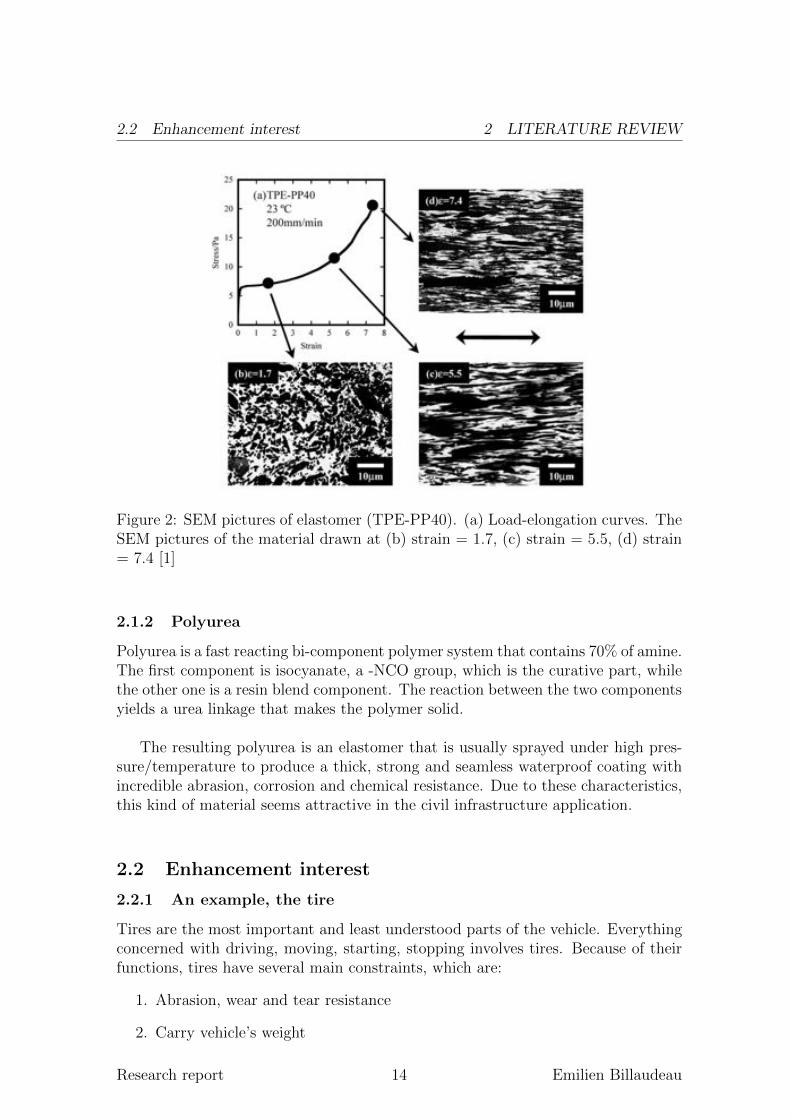
2 SEM pictures of elastomer (TPE-PP40). (a) Load-elongation curves.The SEM pictures of the material drawn at (b) strain = 1.7, (c) strain= 5.5, (d) strain = 7.4 [1] . . . . . . . . . . . . . . . . . . . . . . . . 14

3 Cut tire (Ref : http://www.aviation-fr.info/avion/pneus.php) . . . . . 154 Multi-wall carbon nanotubes (MWNTs) [6] . . . . . . . . . . . . . . . 165 CVD method (Ref : http://ipn2.epfl.ch/CHBU/NTproduction1.htm) . 176 Graphene sheet . . . . . . . . . . . . . . . . . . . . . . . . . . . . . . 187 SEM picture of graphene nanoplatelets (Ref : http://www.xgscience.com/

products.html) . . . . . . . . . . . . . . . . . . . . . . . . . . . . . . . 188 CNTs network for polymer-based nanocomposites (Ref : http://www.nano-

lab.com/) . . . . . . . . . . . . . . . . . . . . . . . . . . . . . . . . . 209 Facilities in the laboratory . . . . . . . . . . . . . . . . . . . . . . . . 2510 Uni-axial tensile test: (a) Strain = 0; (b) Strain = 400% . . . . . . . 2611 Matlab smoothing (1 wt% (CNTs)) . . . . . . . . . . . . . . . . . . . 2712 Experimental data used for the MCalibration optimization . . . . . . 2813 MCalibration program (material model optimization) . . . . . . . . . 2914 MCalibration optimization result, Engineering stress (MPa) / Engi-

neering strain . . . . . . . . . . . . . . . . . . . . . . . . . . . . . . . 3015 Abaqus input file (MCalibration exported data) . . . . . . . . . . . . 3016 Boundary conditions in Abaqus . . . . . . . . . . . . . . . . . . . . . 3117 Sample deformation in the Abaqus calculation (1st node coordinate) . 3218 Nanoparticles visualization: (a) CNTs (Magnification x25000); (b)

GNPs (Magnification x787) . . . . . . . . . . . . . . . . . . . . . . . 3419 1st protocol results, Engineering stress (MPa) / Engineering strain . 3520 First protocol samples: (a) Aqualine 300 picture; (b) Aqualine 300 +

THF + 1 wt% of CNTs picture; (c) Aqualine 300 + THF + 1 wt% ofCNTs SEM picture (Magnification x100); (d) Aqualine 300 + THF+ 1 wt% of CNTs SEM picture (Magnification x6000) . . . . . . . . . 36

21 2nd protocol results, Engineering stress (MPa) / Engineering strain . 3722 2nd protocol results: (a) maximum strain / wt%(CNTs); (b) ultimate

stress (MPa) / wt%(CNTs) . . . . . . . . . . . . . . . . . . . . . . . 3823 Nanocomposite (0.5 wt% of CNTs), interaction CNT/Matrix (Mag-

nification x25000) . . . . . . . . . . . . . . . . . . . . . . . . . . . . . 3924 2nd protocol results, Engineering stress (MPa) / Engineering strain . 4025 2nd protocol results: (a) maximum strain / wt%(GNPs); (b) ultimate

stress (MPa) / wt%(GNPs) . . . . . . . . . . . . . . . . . . . . . . . 4126 Comparison , Engineering stress (MPa) / Engineering strain . . . . . 4227 Ogden model parameters and interpolation (parameter value / wt%(CNTs)):

(a) Mu1; (b) Alpha1; (c) Mu2; (d) Alpha2 . . . . . . . . . . . . . . . 4528 Photo of CNTs mechanically stirred in a solvent (THF) . . . . . . . . 50


LIST OF FIGURES LIST OF FIGURES

29 (a) Ultrasonic stirring by using a Sonicator hielscher UP50H ; (b)Comparison of stirring methods : Ultrasonic (left) / Mechanical stir-ring (right) . . . . . . . . . . . . . . . . . . . . . . . . . . . . . . . . 51

30 (a) Sonicated CNTs (Magnification x283); (b) Original CNTs (Mag-nification x300); (c) Sonicated CNTs (Magnification x2500); (d) Orig-inal CNTs (Magnification x30000) . . . . . . . . . . . . . . . . . . . . 52

31 Centrifuge Sorvall LEGEND X1 : filtration of the solutions to high-light the solvent effect in the CNTs dispersion . . . . . . . . . . . . . 52

32 Solvent comparison after sonicator and centrifuge steps(0.34 g ofCNTs in 40 ml of solvent) From left to right : Distilled water, THF,

Ethanol . . . . . . . . . . . . . . . . . . . . . . . . . . . . . . . . . . 5333 Solvent comparison after sonicator and centrifuge steps(34 mg of

CNTs in 40 ml of solvent) From left to right : THF, Distilled wa-

ter . . . . . . . . . . . . . . . . . . . . . . . . . . . . . . . . . . . . . 5334 THF or distilled water in the matrix? From left to right : THF,

Distilled water . . . . . . . . . . . . . . . . . . . . . . . . . . . . . . . 5435 Behavior prediction, Engineering stress (MPa) / Engineering strain

(a) Strain rate = 0.02 ; (b) Strain rate = 0.2; (c) Strain rate = 0.5;(d) Strain rate = 2 . . . . . . . . . . . . . . . . . . . . . . . . . . . . 55

36 Modeling method using a MCalibration input file . . . . . . . . . . . 56


LIST OF TABLES LIST OF TABLES

List of Tables

1 CNTs properties . . . . . . . . . . . . . . . . . . . . . . . . . . . . . 172 Comparison between CNTs and GNPs mechanical properties . . . . . 193 Nanocomposite compositions . . . . . . . . . . . . . . . . . . . . . . . 234 CNT-based composite properties . . . . . . . . . . . . . . . . . . . . 385 GNP-based composite properties . . . . . . . . . . . . . . . . . . . . 416 Ogden parameters for the CNT nanocomposite modeling . . . . . . . 437 Hyperfoam parameters for the GNP nanocomposite modeling . . . . . 44


1 INTRODUCTION

1 Introduction

Protection of civil infrastructure from environmental and aging deterioration andother extreme conditions is a key concern in any country and particularly in theUnited States[12]. In many urban cities, counties and states, the infrastructure suf-fers from corrosion, deterioration of structural elements due to climate and environ-mental changes, damage induced by wind or earthquake excitations or by man-madeaction, aging of materials and many more.

These issues require continuous monitoring, repairs and the strengthening andreplacement of damaged components. All of these actions require significant resourceallocation for maintenance. The development of new technologies and new materialsoffers an innovative route to solve some of the problems that currently afflict our in-frastructural system. Recently, the production and use of nanoparticles has becomea major research theme worldwide5. Many applications of these nanoparticles relyon their incorporation into a host matrix to form the so called nanocomposite6. Theterm ”nanocomposite” is usually used to describe multiphase solid materials whereat least one of the phases is in orders of nanometers. This project consists in thenanoenhancement study in order to find a suitable manufacturing protocol and anoptimum of the enhancement amount for the studied nanocomposites.

5Bibliography work in appendix (French document)

6The bibliography section will introduce these new materials and their properties


2 LITERATURE REVIEW

2 Literature review

Introducing the context of the study, this literature review describes the enhance-ment interest in polymer materials. Presenting several functions and properties ofthe materials involved in the composite and nanocomposite structure, this sectionhighlights some theories on these complex materials.


2.1 Elastomer presentation 2 LITERATURE REVIEW

2.1 Elastomer presentation

2.1.1 Mechanical properties

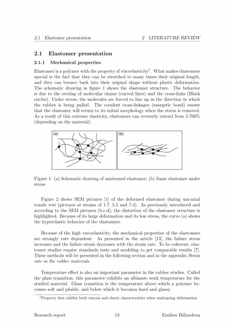
Elastomer is a polymer with the property of viscoelasticity7. What makes elastomersspecial is the fact that they can be stretched to many times their original length,and they can bounce back into their original shape without plastic deformation.The schematic drawing in figure 1 shows the elastomer structure. The behavioris due to the overlap of molecular chains (curved lines) and the cross-links (Blackcircles). Under stress, the molecules are forced to line up in the direction in whichthe rubber is being pulled. The covalent cross-linkages (energetic bond) ensurethat the elastomer will return to its initial morphology when the stress is removed.As a result of this extreme elasticity, elastomers can reversely extend from 5-700%(depending on the material).

Figure 1: (a) Schematic drawing of unstressed elastomer; (b) Same elastomer understress

Figure 2 shows SEM pictures [1] of the deformed elastomer during uni-axialtensile test (pictures at strains of 1.7, 5.5 and 7.4). As previously introduced andaccording to the SEM pictures (b,c,d), the distortion of the elastomer structure ishighlighted. Because of its large deformation and its low stress, the curve (a) showsthe hyperelastic behavior of the elastomers.

Because of the high viscoelasticity, the mechanical properties of the elastomersare strongly rate dependent. As presented in the article [13], the failure stressincreases and the failure strain decreases with the strain rate. To be coherent, elas-tomer studies require standards tests and modeling to get comparable results [7].These methods will be presented in the following section and in the appendix Strain

rate in the rubber materials.

Temperature effect is also an important parameter in the rubber studies. Calledthe glass transition, this parameter exhibits an ultimate work temperature for thestudied material. Glass transition is the temperature above which a polymer be-comes soft and pliable, and below which it becomes hard and glassy.

7Property that exhibit both viscous and elastic characteristics when undergoing deformation


2.2 Enhancement interest 2 LITERATURE REVIEW

Figure 2: SEM pictures of elastomer (TPE-PP40). (a) Load-elongation curves. TheSEM pictures of the material drawn at (b) strain = 1.7, (c) strain = 5.5, (d) strain= 7.4 [1]

2.1.2 Polyurea

Polyurea is a fast reacting bi-component polymer system that contains 70% of amine.The first component is isocyanate, a -NCO group, which is the curative part, whilethe other one is a resin blend component. The reaction between the two componentsyields a urea linkage that makes the polymer solid.

The resulting polyurea is an elastomer that is usually sprayed under high pres-sure/temperature to produce a thick, strong and seamless waterproof coating withincredible abrasion, corrosion and chemical resistance. Due to these characteristics,this kind of material seems attractive in the civil infrastructure application.

2.2 Enhancement interest

2.2.1 An example, the tire

Tires are the most important and least understood parts of the vehicle. Everythingconcerned with driving, moving, starting, stopping involves tires. Because of theirfunctions, tires have several main constraints, which are:

1. Abrasion, wear and tear resistance

2. Carry vehicle’s weight


2.2 Enhancement interest 2 LITERATURE REVIEW

3. Transmit forces

4. Withstand shocks

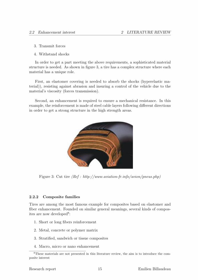
In order to get a part meeting the above requirements, a sophisticated materialstructure is needed. As shown in figure 3, a tire has a complex structure where eachmaterial has a unique role.

First, an elastomer covering is needed to absorb the shocks (hyperelastic ma-terial)), resisting against abrasion and insuring a control of the vehicle due to thematerial’s viscosity (forces transmission).

Second, an enhancement is required to ensure a mechanical resistance. In thisexample, the reinforcement is made of steel cable layers following different directionsin order to get a strong structure in the high strength areas.

Figure 3: Cut tire (Ref : http://www.aviation-fr.info/avion/pneus.php)

2.2.2 Composite families

Tires are among the most famous example for composites based on elastomer andfiber enhancement. Founded on similar general meanings, several kinds of compos-ites are now developed8:

1. Short or long fibers reinforcement

2. Metal, concrete or polymer matrix

3. Stratified, sandwich or tissue composites

4. Macro, micro or nano enhancement

8These materials are not presented in this literature review, the aim is to introduce the com-

posite interest


2.3 Carbon nanotubes 2 LITERATURE REVIEW

Nano-reinforcement is currently under consideration. The three sections belowpresent these new composites with their interests. This review introduces severalsnano-enhancements and the nanocomposite’s expected properties.

2.3 Carbon nanotubes

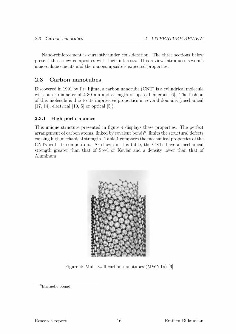
Discovered in 1991 by Pr. Iijima, a carbon nanotube (CNT) is a cylindrical moleculewith outer diameter of 4-30 nm and a length of up to 1 microns [6]. The fashionof this molecule is due to its impressive properties in several domains (mechanical[17, 14], electrical [10, 5] or optical [5]).

2.3.1 High performances

This unique structure presented in figure 4 displays these properties. The perfectarrangement of carbon atoms, linked by covalent bonds9, limits the structural defectscausing high mechanical strength. Table 1 compares the mechanical properties of theCNTs with its competitors. As shown in this table, the CNTs have a mechanicalstrength greater than that of Steel or Kevlar and a density lower than that ofAluminum.

Figure 4: Multi-wall carbon nanotubes (MWNTs) [6]

9Energetic bound


2.4 Graphene Nanoplatelets 2 LITERATURE REVIEW

Properties CNTs Competitors

Young Modulus 1 TPa Steel : 200 GPaTensile Strength 45 GPa Kevlar : 3.5 GPaDensity 1.3 g/cm3 Aluminum : 2.7 g/cm3

Table 1: CNTs properties

2.3.2 Growing methods

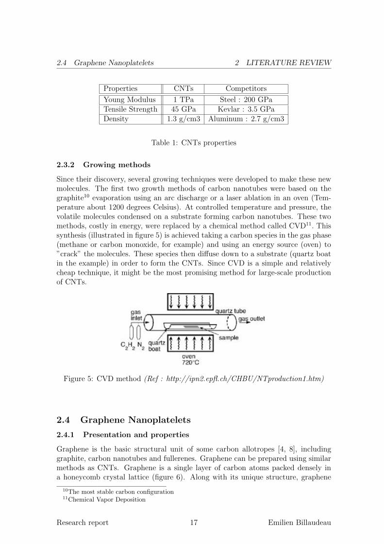
Since their discovery, several growing techniques were developed to make these newmolecules. The first two growth methods of carbon nanotubes were based on thegraphite10 evaporation using an arc discharge or a laser ablation in an oven (Tem-perature about 1200 degrees Celsius). At controlled temperature and pressure, thevolatile molecules condensed on a substrate forming carbon nanotubes. These twomethods, costly in energy, were replaced by a chemical method called CVD11. Thissynthesis (illustrated in figure 5) is achieved taking a carbon species in the gas phase(methane or carbon monoxide, for example) and using an energy source (oven) to”crack” the molecules. These species then diffuse down to a substrate (quartz boatin the example) in order to form the CNTs. Since CVD is a simple and relativelycheap technique, it might be the most promising method for large-scale productionof CNTs.

Figure 5: CVD method (Ref : http://ipn2.epfl.ch/CHBU/NTproduction1.htm)

2.4 Graphene Nanoplatelets

2.4.1 Presentation and properties

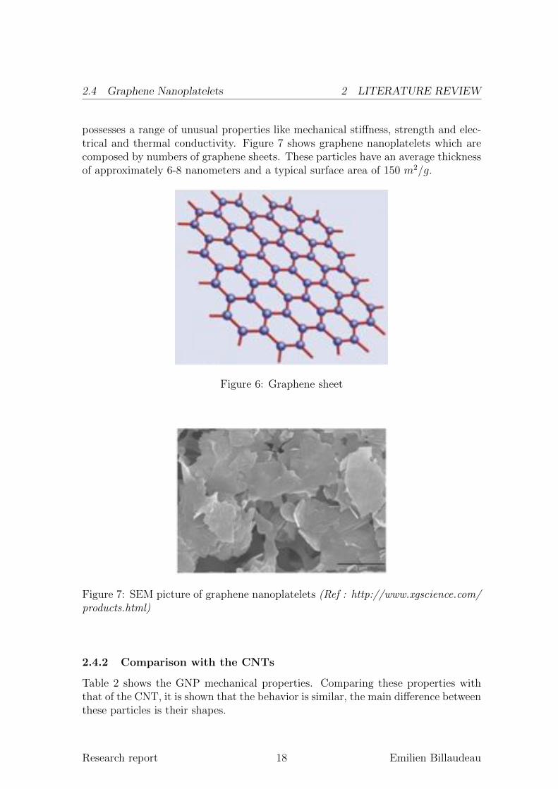
Graphene is the basic structural unit of some carbon allotropes [4, 8], includinggraphite, carbon nanotubes and fullerenes. Graphene can be prepared using similarmethods as CNTs. Graphene is a single layer of carbon atoms packed densely ina honeycomb crystal lattice (figure 6). Along with its unique structure, graphene

10The most stable carbon configuration

11Chemical Vapor Deposition


2.4 Graphene Nanoplatelets 2 LITERATURE REVIEW

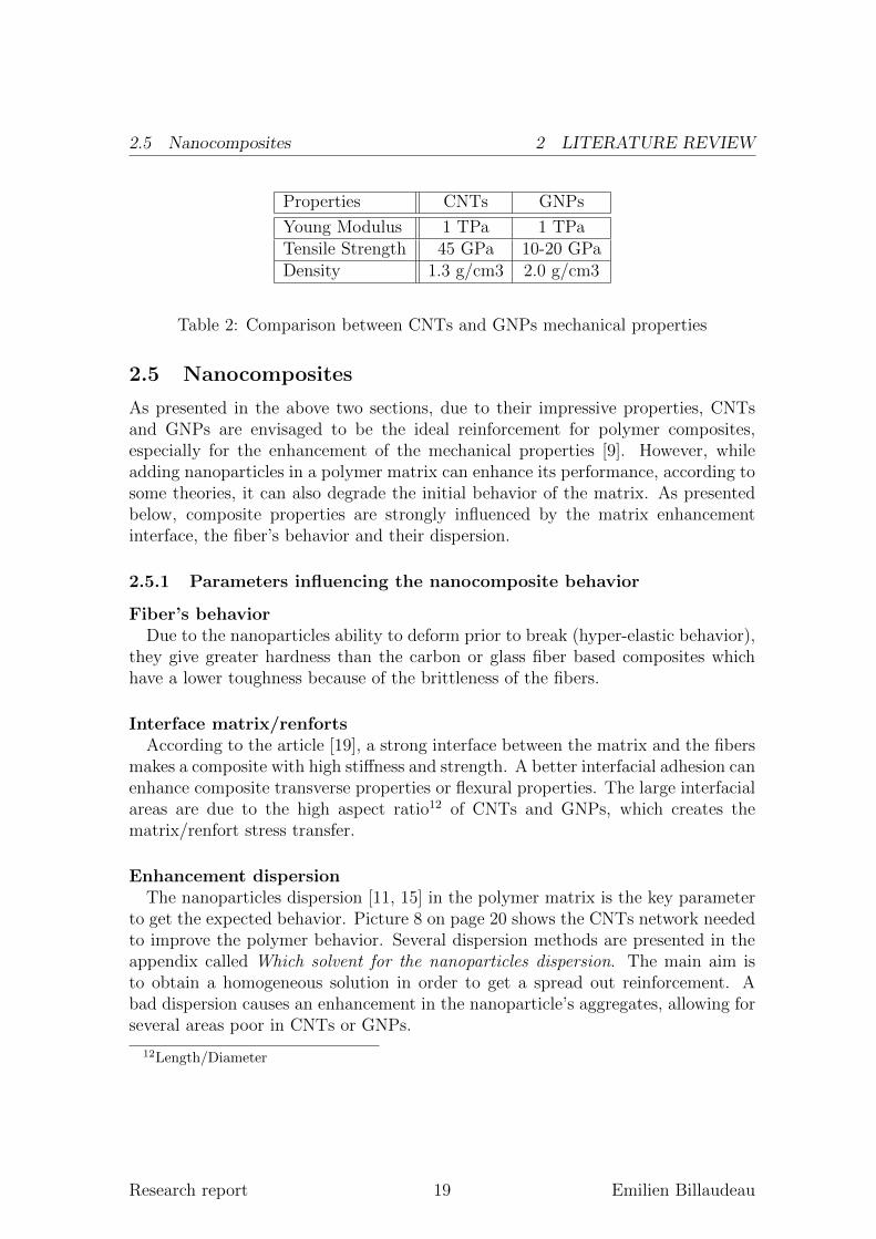
possesses a range of unusual properties like mechanical stiffness, strength and elec-trical and thermal conductivity. Figure 7 shows graphene nanoplatelets which arecomposed by numbers of graphene sheets. These particles have an average thicknessof approximately 6-8 nanometers and a typical surface area of 150 m2/g.

Figure 6: Graphene sheet

Figure 7: SEM picture of graphene nanoplatelets (Ref : http://www.xgscience.com/

products.html)

2.4.2 Comparison with the CNTs

Table 2 shows the GNP mechanical properties. Comparing these properties withthat of the CNT, it is shown that the behavior is similar, the main difference betweenthese particles is their shapes.


2.5 Nanocomposites 2 LITERATURE REVIEW

Properties CNTs GNPs

Young Modulus 1 TPa 1 TPaTensile Strength 45 GPa 10-20 GPaDensity 1.3 g/cm3 2.0 g/cm3

Table 2: Comparison between CNTs and GNPs mechanical properties

2.5 Nanocomposites

As presented in the above two sections, due to their impressive properties, CNTsand GNPs are envisaged to be the ideal reinforcement for polymer composites,especially for the enhancement of the mechanical properties [9]. However, whileadding nanoparticles in a polymer matrix can enhance its performance, according tosome theories, it can also degrade the initial behavior of the matrix. As presentedbelow, composite properties are strongly influenced by the matrix enhancementinterface, the fiber’s behavior and their dispersion.

2.5.1 Parameters influencing the nanocomposite behavior

Fiber’s behaviorDue to the nanoparticles ability to deform prior to break (hyper-elastic behavior),

they give greater hardness than the carbon or glass fiber based composites whichhave a lower toughness because of the brittleness of the fibers.

Interface matrix/renfortsAccording to the article [19], a strong interface between the matrix and the fibers

makes a composite with high stiffness and strength. A better interfacial adhesion canenhance composite transverse properties or flexural properties. The large interfacialareas are due to the high aspect ratio12 of CNTs and GNPs, which creates thematrix/renfort stress transfer.

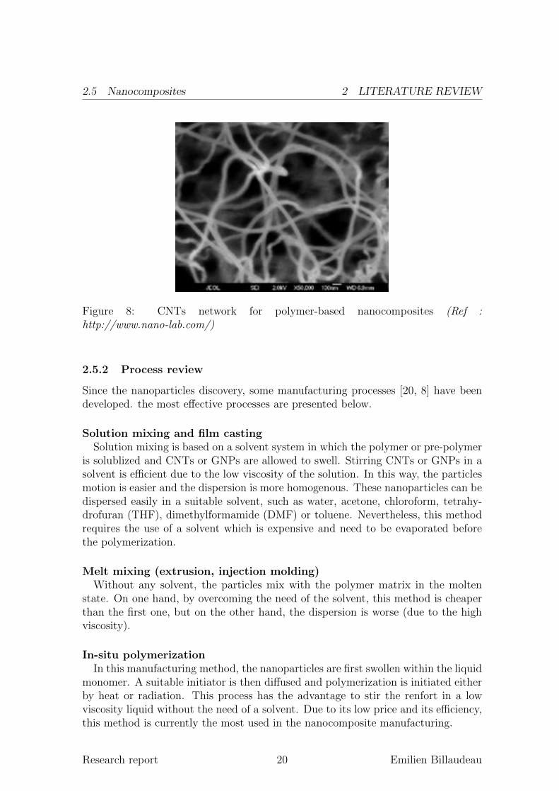
Enhancement dispersionThe nanoparticles dispersion [11, 15] in the polymer matrix is the key parameter

to get the expected behavior. Picture 8 on page 20 shows the CNTs network neededto improve the polymer behavior. Several dispersion methods are presented in theappendix called Which solvent for the nanoparticles dispersion. The main aim isto obtain a homogeneous solution in order to get a spread out reinforcement. Abad dispersion causes an enhancement in the nanoparticle’s aggregates, allowing forseveral areas poor in CNTs or GNPs.

12Length/Diameter


2.5 Nanocomposites 2 LITERATURE REVIEW

Figure 8: CNTs network for polymer-based nanocomposites (Ref :

http://www.nano-lab.com/)

2.5.2 Process review

Since the nanoparticles discovery, some manufacturing processes [20, 8] have beendeveloped. the most effective processes are presented below.

Solution mixing and film castingSolution mixing is based on a solvent system in which the polymer or pre-polymer

is solublized and CNTs or GNPs are allowed to swell. Stirring CNTs or GNPs in asolvent is efficient due to the low viscosity of the solution. In this way, the particlesmotion is easier and the dispersion is more homogenous. These nanoparticles can bedispersed easily in a suitable solvent, such as water, acetone, chloroform, tetrahy-drofuran (THF), dimethylformamide (DMF) or toluene. Nevertheless, this methodrequires the use of a solvent which is expensive and need to be evaporated beforethe polymerization.

Melt mixing (extrusion, injection molding)Without any solvent, the particles mix with the polymer matrix in the molten

state. On one hand, by overcoming the need of the solvent, this method is cheaperthan the first one, but on the other hand, the dispersion is worse (due to the highviscosity).

In-situ polymerizationIn this manufacturing method, the nanoparticles are first swollen within the liquid

monomer. A suitable initiator is then diffused and polymerization is initiated eitherby heat or radiation. This process has the advantage to stir the renfort in a lowviscosity liquid without the need of a solvent. Due to its low price and its efficiency,this method is currently the most used in the nanocomposite manufacturing.


3 MATERIALS AND METHODS

3 Materials and methods

This section presents the methods used to conduct the research. The subsectionsthat follow explain the materials used to perform the study; the several protocolsfound to make the nanocomposites; the tests completed to describe the nanocompos-ite’s behavior and the hyperelastic modeling used to predict the general performanceof this kind of composite.


3.1 Manufacturing and experimental tests 3 MATERIALS AND METHODS

3.1 Manufacturing and experimental tests

3.1.1 Materials manufacturing

Materials usedThe Multi-Walled Carbon nanotubes (CNTs) used in this study were purchased

from Sigma Aldrich and were synthetized by Catalitic Chemical Vapor Deposition(CVD).

The Graphene Naoplatelets (GNPs) xGnP-M-15 were purchased from XG Sci-ence, Inc. and were also synthetized by CVD.

The Polyurea used in this study was ordered from ITW Futura Coatings asAqualine 300 and from ITW Devcon as Flexane 80 liquid 15800 (equivalent to theAqualine 300).

Tetrahydrofuran (THF) anhydrous was purchased from Sigma Aldrich. This isan organic solvent that is used to disperse CNTs in the polymer matrix. Ethanoland distilled water were also used as solvent in the nanoparticles dispersion.

The nanocomposite specimens have been prepared by adding different quantitiesin weight percentage [wt%] of nanoparticles (CNTs or GSs) as follows:

1. Polyurea

2. Polyurea + solvent + 0.1 wt% (CNTs or GNPs)


4. Polyurea + solvent + 1 wt% (CNTs or GNPs)





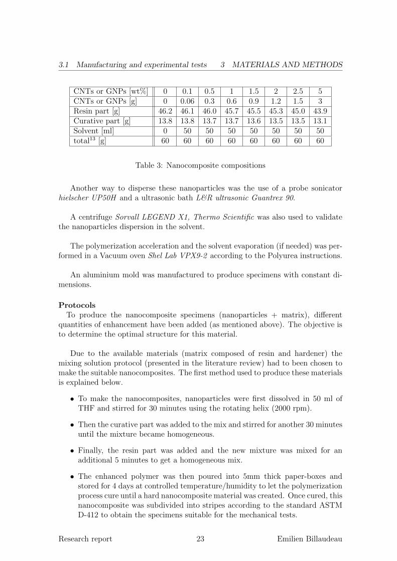
Table 3 indicates the needed quantities to manufacture the different nanocom-posites (around 30 g per sample).

One of the main goals is to evaluate which of the above mentioned nanocompos-ites yields the best overall mechanical performance.

InstrumentationThe nanoparticles dispersion was performed mixing the solution with a rotative

helix IKA RW 20 digital.



CNTs or GNPs [wt%] 0 0.1 0.5 1 1.5 2 2.5 5CNTs or GNPs [g] 0 0.06 0.3 0.6 0.9 1.2 1.5 3Resin part [g] 46.2 46.1 46.0 45.7 45.5 45.3 45.0 43.9Curative part [g] 13.8 13.8 13.7 13.7 13.6 13.5 13.5 13.1Solvent [ml] 0 50 50 50 50 50 50 50total13 [g] 60 60 60 60 60 60 60 60

Table 3: Nanocomposite compositions

Another way to disperse these nanoparticles was the use of a probe sonicatorhielscher UP50H and a ultrasonic bath L&R ultrasonic Guantrex 90.

A centrifuge Sorvall LEGEND X1, Thermo Scientific was also used to validatethe nanoparticles dispersion in the solvent.

The polymerization acceleration and the solvent evaporation (if needed) was per-formed in a Vacuum oven Shel Lab VPX9-2 according to the Polyurea instructions.

An aluminium mold was manufactured to produce specimens with constant di-mensions.

ProtocolsTo produce the nanocomposite specimens (nanoparticles + matrix), different

quantities of enhancement have been added (as mentioned above). The objective isto determine the optimal structure for this material.

Due to the available materials (matrix composed of resin and hardener) themixing solution protocol (presented in the literature review) had to been chosen tomake the suitable nanocomposites. The first method used to produce these materialsis explained below.

• To make the nanocomposites, nanoparticles were first dissolved in 50 ml ofTHF and stirred for 30 minutes using the rotating helix (2000 rpm).

• Then the curative part was added to the mix and stirred for another 30 minutesuntil the mixture became homogeneous.

• Finally, the resin part was added and the new mixture was mixed for anadditional 5 minutes to get a homogeneous mix.

• The enhanced polymer was then poured into 5mm thick paper-boxes andstored for 4 days at controlled temperature/humidity to let the polymerizationprocess cure until a hard nanocomposite material was created. Once cured, thisnanocomposite was subdivided into stripes according to the standard ASTMD-412 to obtain the specimens suitable for the mechanical tests.



With the results found, the method had to be changed. In fact, the main pointin the nanocomposite research was the nanoparticles dispersion in the matrix. Anefficient method that needed an ultrasonic processor was used to get better results[11]. We also used an aluminum mold to get better precision in the specimen’sdimensions. The improved protocol follows.

• Like the first protocol, the nanoparticles were first dissolved in 50 ml of solvent(chose from a study presented in the appendix) and stirred for 45 minutes usingthe probe sonicator (Frequency : 30 kHz, Amplitude : 100 %, Cycle : 0.914). Itis known that the ultra-sons are efficient for the dispersion, but it is also knownthat the ultra-sons damage the CNTs (after 1 hour the CNTs are 2 micrometershorter). Balanced between a good dispersion (needed for the nanocompositeenhancement) and good nanoparticle’s geometry (also useful to have a betterload transfer in the matrix), this step is one of the most important in themanufacturing.

• This solution was heated in order to evaporate the solvent and to keep only thenanoparticles unagglomerated (very thin powder). At controlled temperature(around the solvent boiling temperature), the solution was heated until thecomplete evaporation of the solvent (controlled by weighing the solution).

• This powder and the resin were stirred for 5 minutes using the rotation helixand then another 15 minutes in the ultrasonic bath.

• Before the casting step, the curative part was added in the solution and stirredfor 5 minutes (around 500 rpm, to avoid creating bubbles). This solution wasthen hand mixed using a spatula to remove as many bubbles as possible. Tofacilitate the release15 after the polymerization process cure (10 hours in themold), the mold was covered with a wax layer.

• 7 days of waiting were necessary to be sure of the properties16 and to obtainthe specimens suitable for the mechanical tests.

3.1.2 Experimental tests

InstrumentationTensile tests were controlled in displacement. According to the ASTM D-412:

”Standard test methods for vulcanized rubber and thermoplastic elastomers - Ten-sion” [7], tension tests were performed using an Instron 30K Universal Testing Ma-chine with a strain rate of 50.8 mm/min (2.00 inch/min). Tested specimen sectionwas measured with a numerical caliper, in order to determine the engineering stressin the material using the tensile machine load measure.

140.9 second on / 0.1 second off

15Polyurea adhesion on the aluminum

16Hardness : 80% after 2 days, 100% after 7 days


3.2 Material modeling 3 MATERIALS AND METHODS

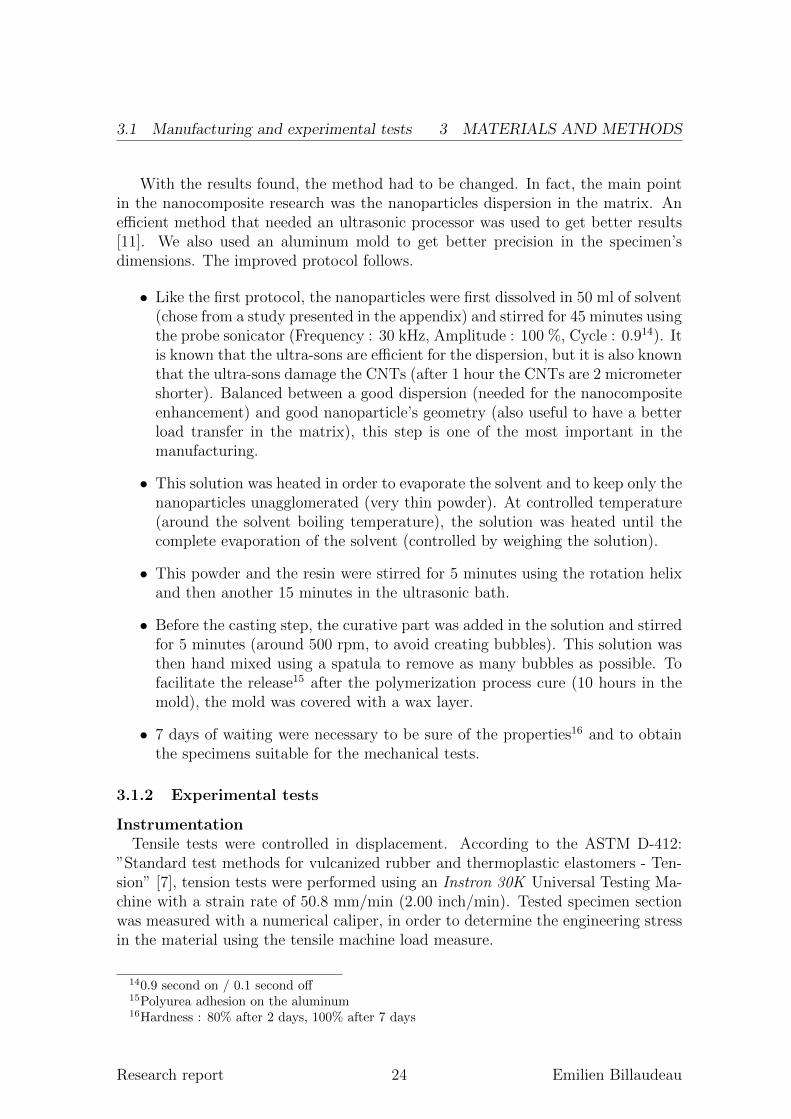
Figure 9: Facilities in the laboratory

Alignment procedure of the tensile machineTensile testing requires a precise mods alignment in order to get an accurate result.

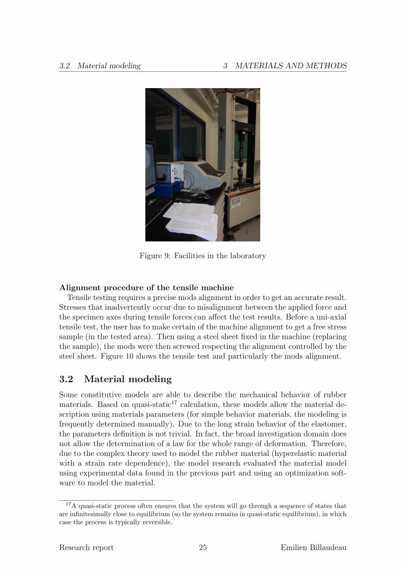
Stresses that inadvertently occur due to misalignment between the applied force andthe specimen axes during tensile forces can affect the test results. Before a uni-axialtensile test, the user has to make certain of the machine alignment to get a free stresssample (in the tested area). Then using a steel sheet fixed in the machine (replacingthe sample), the mods were then screwed respecting the alignment controlled by thesteel sheet. Figure 10 shows the tensile test and particularly the mods alignment.

3.2 Material modeling

Some constitutive models are able to describe the mechanical behavior of rubbermaterials. Based on quasi-static17 calculation, these models allow the material de-scription using materials parameters (for simple behavior materials, the modeling isfrequently determined manually). Due to the long strain behavior of the elastomer,the parameters definition is not trivial. In fact, the broad investigation domain doesnot allow the determination of a law for the whole range of deformation. Therefore,due to the complex theory used to model the rubber material (hyperelastic materialwith a strain rate dependence), the model research evaluated the material modelusing experimental data found in the previous part and using an optimization soft-ware to model the material.

17A quasi-static process often ensures that the system will go through a sequence of states that

are infinitesimally close to equilibrium (so the system remains in quasi-static equilibrium), in which

case the process is typically reversible.



(a) (b)

Figure 10: Uni-axial tensile test: (a) Strain = 0; (b) Strain = 400%

The main goal of this study is to achieve a parametric determination for severalnanocomposites, in order to find a general model.

3.2.1 Modeling using an MCalibration optimization

What is MCalibration?Developed by Jorgen Bergstrom18, MCalibration is a material evaluation software

using experimental data. Due to its many material models [2] and their algorithms,this program is suitable for our modeling. Some sophisticated models are available inthis software. The respective algorithms19 are based on the comparison between themodel curve and experimental data curve, in order to reduce this gap by changingthe model parameters.

The way to use MCalibrationThe first modeling step is based on the experimental data treatment in order to

use them in the MCalibration optimization. To get an efficient material evaluation,the experimental stress/strain curves had to be smoothed. Figure 11 presents theMatlab smoothing. The appendix Matlab smoothing program shows the program.

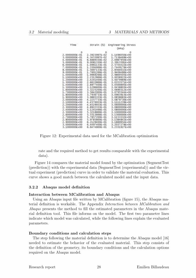
Figure 12 presents the experimental data used as the MCalibration input file.

18MIT Ph.D., Veryst Engineering

19By choice, the algorithms are not presented in this report, they are introduced in the article

[2]



Figure 11: Matlab smoothing (1 wt% (CNTs))

Due to the strain rate20 of the studied material, the time for each increment needsto be quantified in order to evaluate the model. This time has been arbitrarily de-termined because of the impossibility of the tensile machine to measure it. The wayto compensate21 this arbitrary time is described in the next paragraph, Interactionbetween MCalibration and Abaqus.

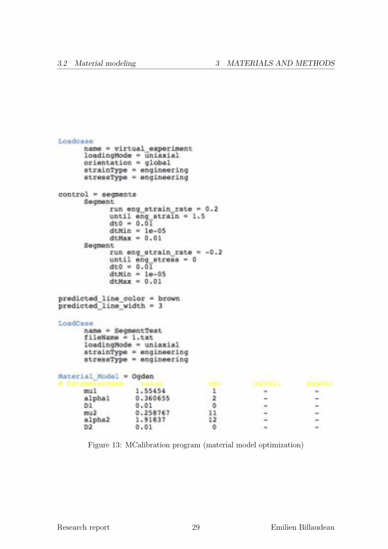
To generate the optimization, some program lines are needed. Figure 13 showsthis MCalibration program [3].

• The second loadcase tells the experimental data used for the material evalu-ation, their meaning (engineering or true values) and the kind of test used toget these results.

• The material model chosen is presented in the MaterialModel section. In theprogram presented in figure 13 on page 29, the studied material model is theOgden model. The following parameters are evaluated using an algorithmdeveloped for this model [2, 3].

• The first loadcase, called virtual experiment, is needed to evaluate the Abaqusresults using the parameters found by the MCalibration evaluation. In thatcase, a cycle was tested (load until 200% of engineering strain, unload until 0MPa of engineering stress). In this section the strain rate was needed to eval-uate the material behavior (the appendix presents the influence of the strain

20dependence on the solicitation speed

21To get comparable results as the experimental tests



Figure 12: Experimental data used for the MCalibration optimization

rate and the required method to get results comparable with the experimentaldata).

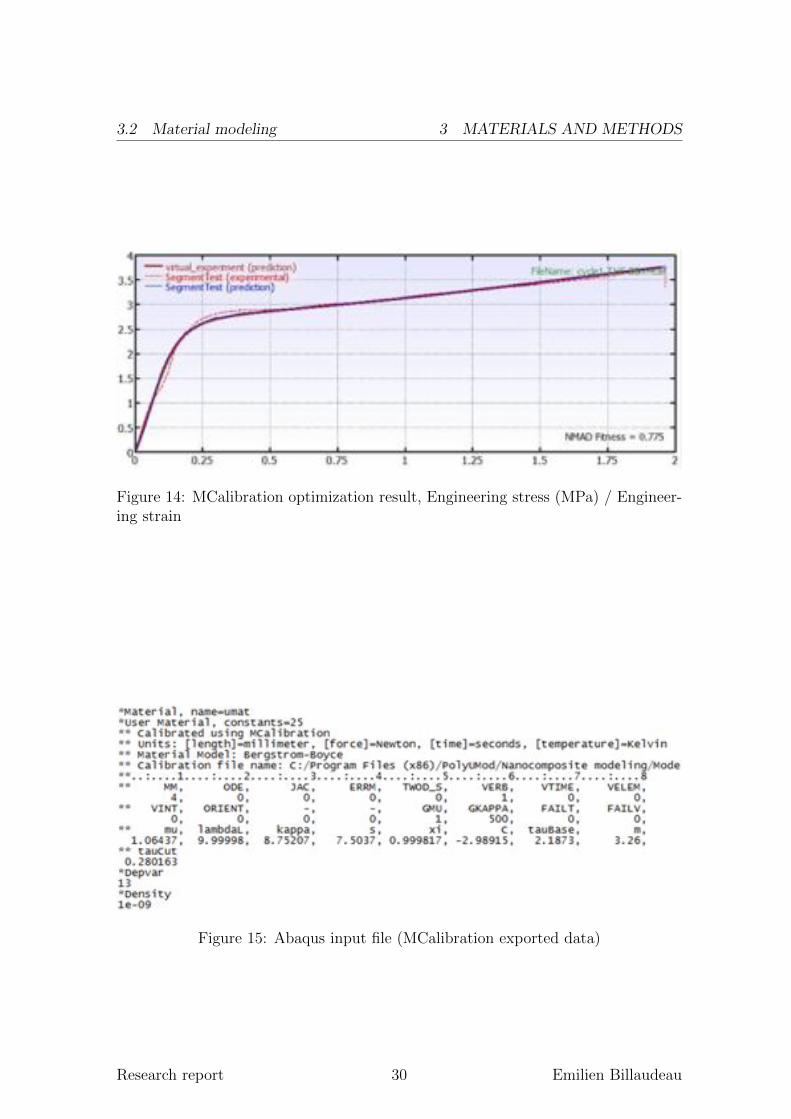
Figure 14 compares the material model found by the optimization (SegmentTest(prediction)) with the experimental data (SegmentTest (experimental)) and the vir-tual experiment (prediction) curve in order to validate the material evaluation. Thiscurve shows a good match between the calculated model and the input data.

3.2.2 Abaqus model definition

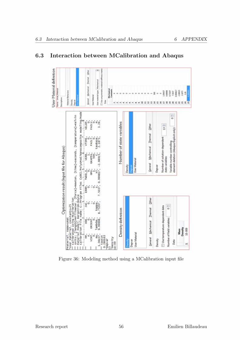
Interaction between MCalibration and AbaqusUsing an Abaqus input file written by MCalibration (figure 15), the Abaqus ma-

terial definition is workable. The Appendix Interaction between MCalibration and

Abaqus presents the method to fill the estimated parameters in the Abaqus mate-rial definition tool. This file informs on the model. The first two parameter linesindicate which model was calculated, while the following lines explain the evaluatedparameters.

Boundary conditions and calculation stepsThe step following the material definition is to determine the Abaqus model [16]

needed to estimate the behavior of the evaluated material. This step consists ofthe definition of the geometry, its boundary conditions and the calculation optionsrequired on the Abaqus model.



Figure 13: MCalibration program (material model optimization)



Figure 14: MCalibration optimization result, Engineering stress (MPa) / Engineer-ing strain

Figure 15: Abaqus input file (MCalibration exported data)



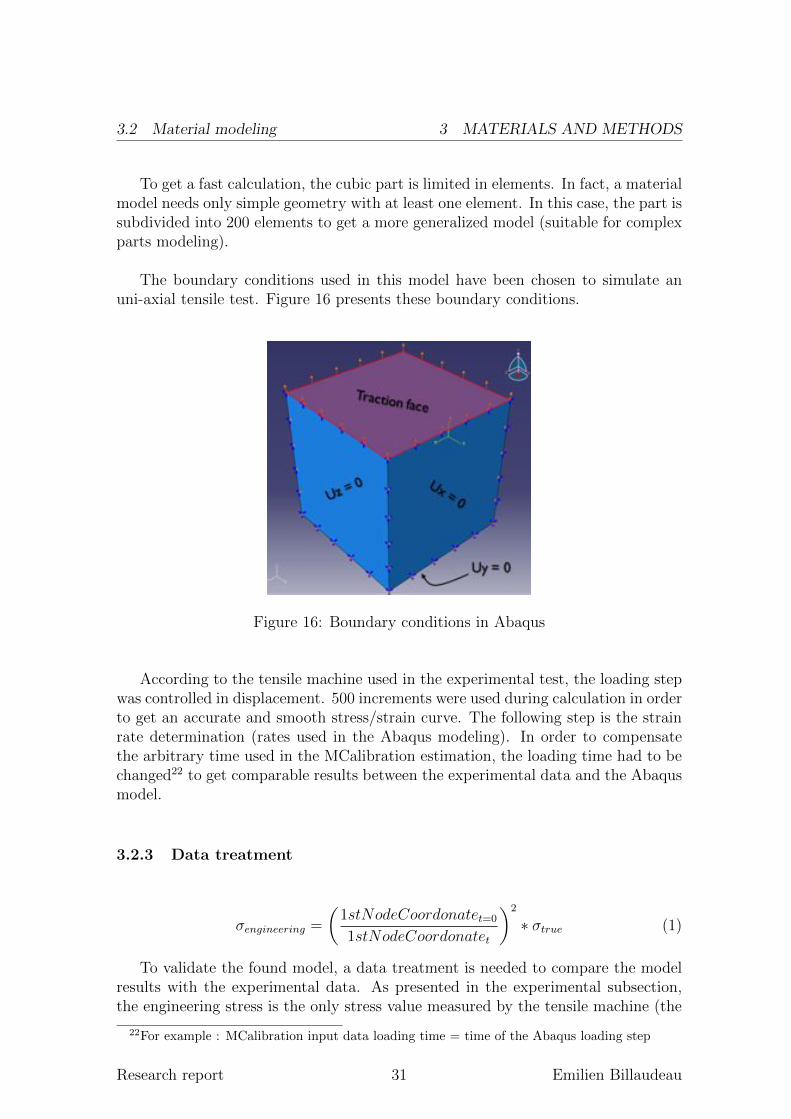
To get a fast calculation, the cubic part is limited in elements. In fact, a materialmodel needs only simple geometry with at least one element. In this case, the part issubdivided into 200 elements to get a more generalized model (suitable for complexparts modeling).

The boundary conditions used in this model have been chosen to simulate anuni-axial tensile test. Figure 16 presents these boundary conditions.

Figure 16: Boundary conditions in Abaqus

According to the tensile machine used in the experimental test, the loading stepwas controlled in displacement. 500 increments were used during calculation in orderto get an accurate and smooth stress/strain curve. The following step is the strainrate determination (rates used in the Abaqus modeling). In order to compensatethe arbitrary time used in the MCalibration estimation, the loading time had to bechanged22 to get comparable results between the experimental data and the Abaqusmodel.

3.2.3 Data treatment

σengineering =

�1stNodeCoordonatet=0

1stNodeCoordonatet

�2

∗ σtrue (1)

To validate the found model, a data treatment is needed to compare the modelresults with the experimental data. As presented in the experimental subsection,the engineering stress is the only stress value measured by the tensile machine (the

22For example : MCalibration input data loading time = time of the Abaqus loading step



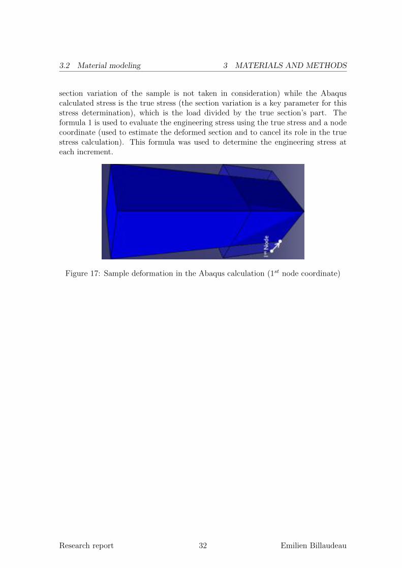
section variation of the sample is not taken in consideration) while the Abaquscalculated stress is the true stress (the section variation is a key parameter for thisstress determination), which is the load divided by the true section’s part. Theformula 1 is used to evaluate the engineering stress using the true stress and a nodecoordinate (used to estimate the deformed section and to cancel its role in the truestress calculation). This formula was used to determine the engineering stress ateach increment.

Figure 17: Sample deformation in the Abaqus calculation (1st node coordinate)


4 RESULTS AND DISCUSSION

4 Results and discussion

This section presents the found results, following the methods presented above.Several nanocomposites were made and tested in the purpose of the behavior pre-diction and enhancement optimum23 research. To perform this study, the sampleswere tested with the tensile machine. Then a fractography analysis followed in orderto investigate the reasons of the noticed behavior. This section also presents themodel determination and the path to find a general model for the tested materials.

23type of enhancement and the amount in the matrix and their amount in the matrix


4.1 Experimental tests 4 RESULTS AND DISCUSSION

4.1 Experimental tests

4.1.1 SEM visualization

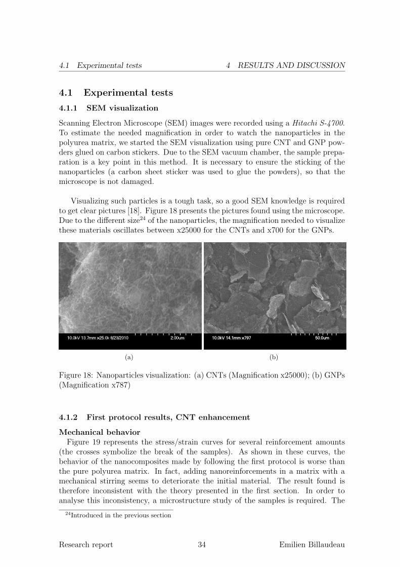
Scanning Electron Microscope (SEM) images were recorded using a Hitachi S-4700.To estimate the needed magnification in order to watch the nanoparticles in thepolyurea matrix, we started the SEM visualization using pure CNT and GNP pow-ders glued on carbon stickers. Due to the SEM vacuum chamber, the sample prepa-ration is a key point in this method. It is necessary to ensure the sticking of thenanoparticles (a carbon sheet sticker was used to glue the powders), so that themicroscope is not damaged.

Visualizing such particles is a tough task, so a good SEM knowledge is requiredto get clear pictures [18]. Figure 18 presents the pictures found using the microscope.Due to the different size24 of the nanoparticles, the magnification needed to visualizethese materials oscillates between x25000 for the CNTs and x700 for the GNPs.

(a) (b)

Figure 18: Nanoparticles visualization: (a) CNTs (Magnification x25000); (b) GNPs(Magnification x787)

4.1.2 First protocol results, CNT enhancement

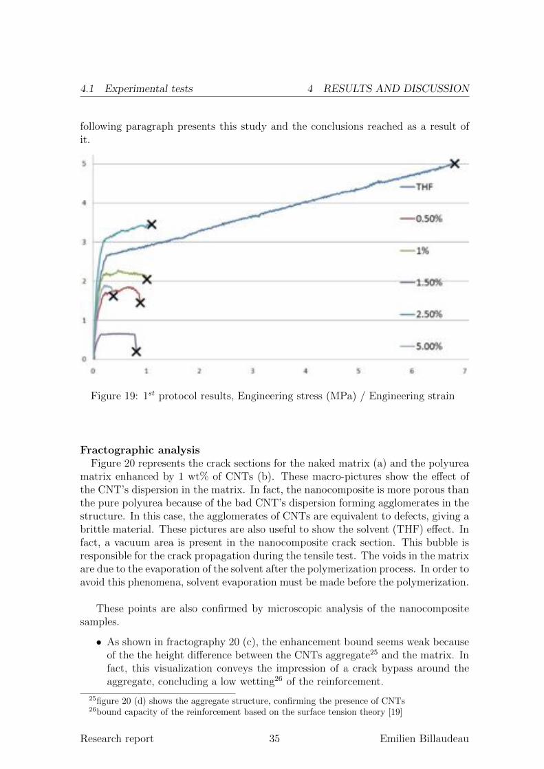
Mechanical behaviorFigure 19 represents the stress/strain curves for several reinforcement amounts

(the crosses symbolize the break of the samples). As shown in these curves, thebehavior of the nanocomposites made by following the first protocol is worse thanthe pure polyurea matrix. In fact, adding nanoreinforcements in a matrix with amechanical stirring seems to deteriorate the initial material. The result found istherefore inconsistent with the theory presented in the first section. In order toanalyse this inconsistency, a microstructure study of the samples is required. The

24Introduced in the previous section



following paragraph presents this study and the conclusions reached as a result ofit.

Figure 19: 1st protocol results, Engineering stress (MPa) / Engineering strain

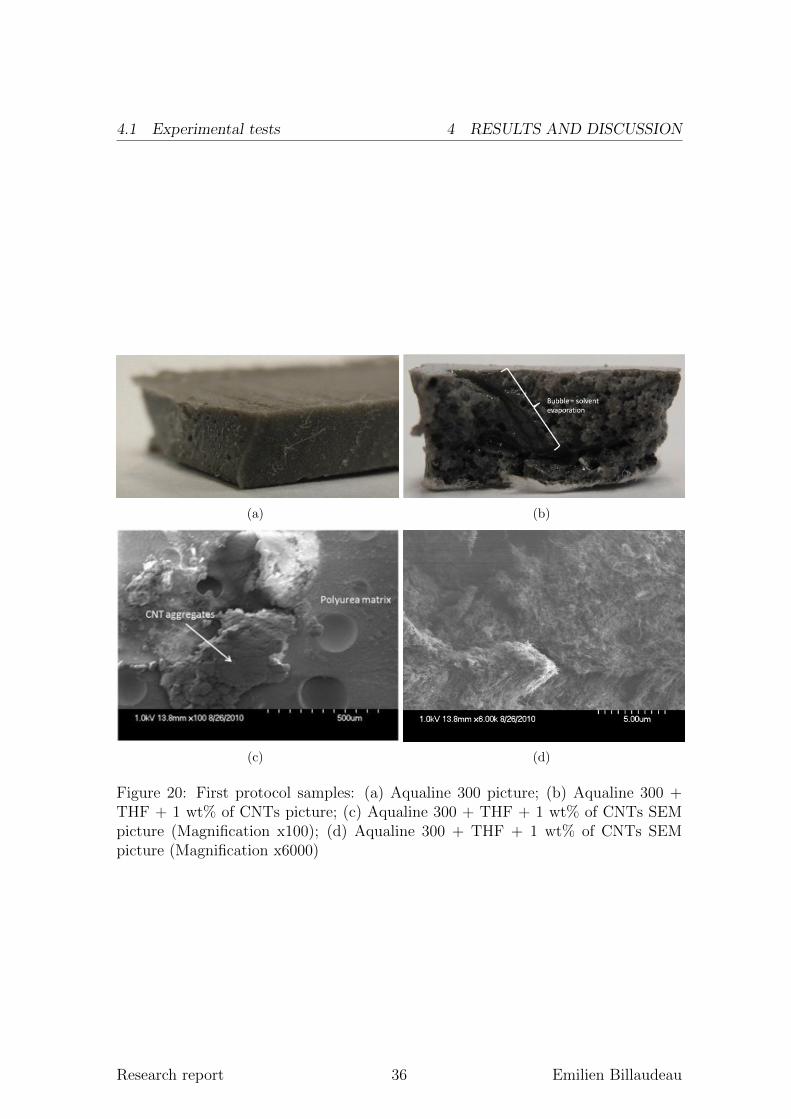
Fractographic analysisFigure 20 represents the crack sections for the naked matrix (a) and the polyurea

matrix enhanced by 1 wt% of CNTs (b). These macro-pictures show the effect ofthe CNT’s dispersion in the matrix. In fact, the nanocomposite is more porous thanthe pure polyurea because of the bad CNT’s dispersion forming agglomerates in thestructure. In this case, the agglomerates of CNTs are equivalent to defects, giving abrittle material. These pictures are also useful to show the solvent (THF) effect. Infact, a vacuum area is present in the nanocomposite crack section. This bubble isresponsible for the crack propagation during the tensile test. The voids in the matrixare due to the evaporation of the solvent after the polymerization process. In order toavoid this phenomena, solvent evaporation must be made before the polymerization.

These points are also confirmed by microscopic analysis of the nanocompositesamples.

• As shown in fractography 20 (c), the enhancement bound seems weak becauseof the the height difference between the CNTs aggregate25 and the matrix. Infact, this visualization conveys the impression of a crack bypass around theaggregate, concluding a low wetting26 of the reinforcement.

25figure 20 (d) shows the aggregate structure, confirming the presence of CNTs

26bound capacity of the reinforcement based on the surface tension theory [19]



(a) (b)

(c) (d)

Figure 20: First protocol samples: (a) Aqualine 300 picture; (b) Aqualine 300 +THF + 1 wt% of CNTs picture; (c) Aqualine 300 + THF + 1 wt% of CNTs SEMpicture (Magnification x100); (d) Aqualine 300 + THF + 1 wt% of CNTs SEMpicture (Magnification x6000)



• Otherwise, the bubble in the matrix assumes the solvent evaporation or afast mechanical stirring. In all cases, this problem degrades the mechanicalbehavior of the material.

4.1.3 Second protocol results, CNT enhancement

Analyzing the results found by using the first protocol, the manufacturing methodhad to be modified. Presented as the second protocol in the subsection 3.3.1, theresults are from tests on materials produced by this method. In this way, this sectionhighlights the nanoparticle’s dispersion effect on the nanocomposite behavior.

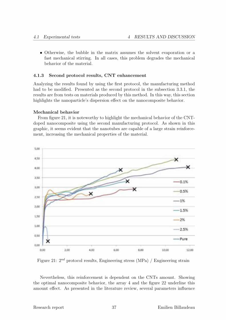
Mechanical behaviorFrom figure 21, it is noteworthy to highlight the mechanical behavior of the CNT-

doped nanocomposite using the second manufacturing protocol. As shown in thisgraphic, it seems evident that the nanotubes are capable of a large strain reinforce-ment, increasing the mechanical properties of the material.

Figure 21: 2nd protocol results, Engineering stress (MPa) / Engineering strain

Nevertheless, this reinforcement is dependent on the CNTs amount. Showingthe optimal nanocomposite behavior, the array 4 and the figure 22 underline thisamount effect. As presented in the literature review, several parameters influence



the nanocomposites. Besides the mechanical behavior of the reinforcement, the en-hanced material behavior also depends on the nanoparticles dispersion [11, 15].

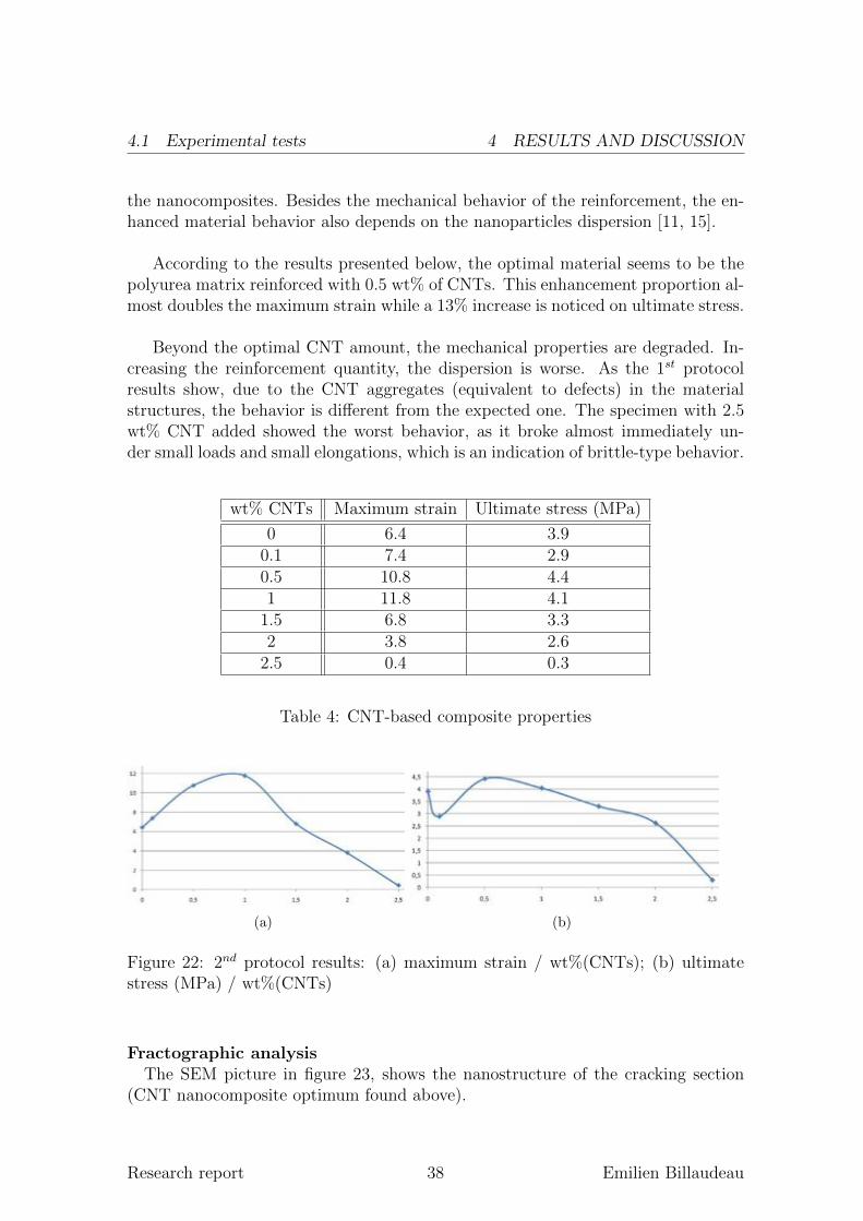
According to the results presented below, the optimal material seems to be thepolyurea matrix reinforced with 0.5 wt% of CNTs. This enhancement proportion al-most doubles the maximum strain while a 13% increase is noticed on ultimate stress.

Beyond the optimal CNT amount, the mechanical properties are degraded. In-creasing the reinforcement quantity, the dispersion is worse. As the 1st protocolresults show, due to the CNT aggregates (equivalent to defects) in the materialstructures, the behavior is different from the expected one. The specimen with 2.5wt% CNT added showed the worst behavior, as it broke almost immediately un-der small loads and small elongations, which is an indication of brittle-type behavior.

wt% CNTs Maximum strain Ultimate stress (MPa)

0 6.4 3.90.1 7.4 2.90.5 10.8 4.41 11.8 4.11.5 6.8 3.32 3.8 2.62.5 0.4 0.3

Table 4: CNT-based composite properties

(a) (b)

Figure 22: 2nd protocol results: (a) maximum strain / wt%(CNTs); (b) ultimatestress (MPa) / wt%(CNTs)

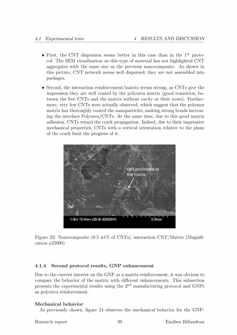
Fractographic analysisThe SEM picture in figure 23, shows the nanostructure of the cracking section

(CNT nanocomposite optimum found above).



• First, the CNT dispersion seems better in this case than in the 1st proto-col. The SEM visualization on this type of material has not highlighted CNTaggregates with the same size as the previous nanocomposite. As shown inthis picture, CNT network seems well dispersed; they are not assembled intopackages.

• Second, the interaction reinforcement/matrix seems strong, as CNTs give theimpression they are well coated by the polyurea matrix (good transition, be-tween the free CNTs and the matrix without cavity at their roots). Further-more, very few CNTs were actually observed, which suggest that the polymermatrix has thoroughly coated the nanoparticles, making strong bonds increas-ing the interface Polyurea/CNTs. At the same time, due to this good matrixadhesion, CNTs retard the crack propagation. Indeed, due to their impressivemechanical properties, CNTs with a vertical orientation relative to the planeof the crack limit the progress of it.

Figure 23: Nanocomposite (0.5 wt% of CNTs), interaction CNT/Matrix (Magnifi-cation x25000)

4.1.4 Second protocol results, GNP enhancement

Due to the current interest on the GNP as a matrix reinforcement, it was obvious tocompare the behavior of the matrix with different enhancements. This subsectionpresents the experimental results using the 2nd manufacturing protocol and GNPsas polyurea reinforcement.

Mechanical behaviorAs previously shown, figure 24 observes the mechanical behavior for the GNP-



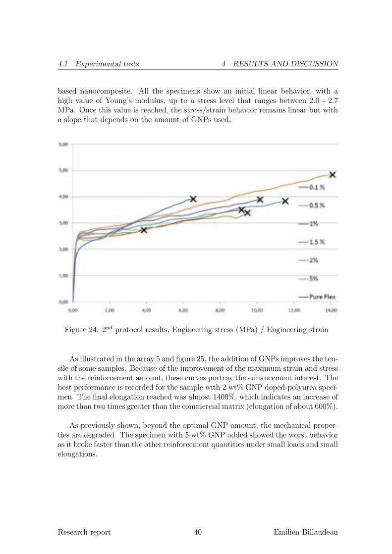
based nanocomposite. All the specimens show an initial linear behavior, with ahigh value of Young’s modulus, up to a stress level that ranges between 2.0 - 2.7MPa. Once this value is reached, the stress/strain behavior remains linear but witha slope that depends on the amount of GNPs used.

Figure 24: 2nd protocol results, Engineering stress (MPa) / Engineering strain

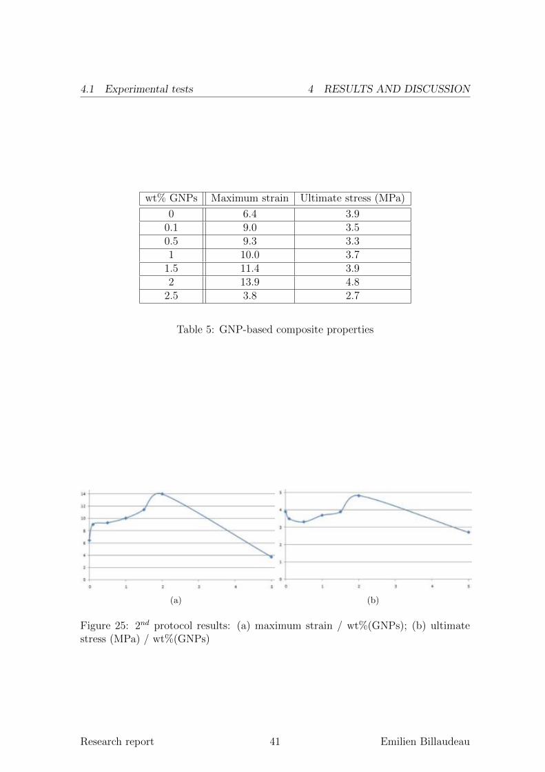
As illustrated in the array 5 and figure 25, the addition of GNPs improves the ten-sile of some samples. Because of the improvement of the maximum strain and stresswith the reinforcement amount, these curves portray the enhancement interest. Thebest performance is recorded for the sample with 2 wt% GNP doped-polyurea speci-men. The final elongation reached was almost 1400%, which indicates an increase ofmore than two times greater than the commercial matrix (elongation of about 600%).

As previously shown, beyond the optimal GNP amount, the mechanical proper-ties are degraded. The specimen with 5 wt% GNP added showed the worst behavioras it broke faster than the other reinforcement quantities under small loads and smallelongations.



wt% GNPs Maximum strain Ultimate stress (MPa)

0 6.4 3.90.1 9.0 3.50.5 9.3 3.31 10.0 3.71.5 11.4 3.92 13.9 4.82.5 3.8 2.7

Table 5: GNP-based composite properties

(a) (b)

Figure 25: 2nd protocol results: (a) maximum strain / wt%(GNPs); (b) ultimatestress (MPa) / wt%(GNPs)



4.1.5 Optimal nanocomposite, amount and enhancement type

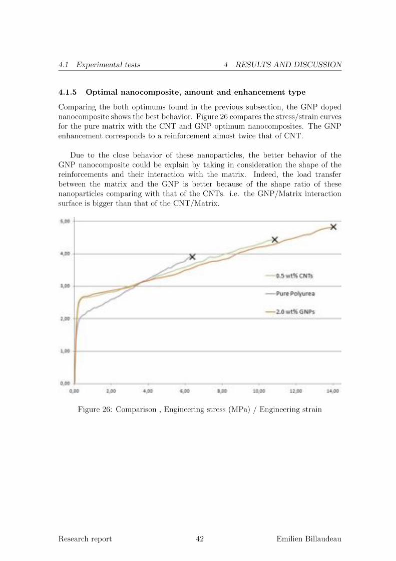
Comparing the both optimums found in the previous subsection, the GNP dopednanocomposite shows the best behavior. Figure 26 compares the stress/strain curvesfor the pure matrix with the CNT and GNP optimum nanocomposites. The GNPenhancement corresponds to a reinforcement almost twice that of CNT.

Due to the close behavior of these nanoparticles, the better behavior of theGNP nanocomposite could be explain by taking in consideration the shape of thereinforcements and their interaction with the matrix. Indeed, the load transferbetween the matrix and the GNP is better because of the shape ratio of thesenanoparticles comparing with that of the CNTs. i.e. the GNP/Matrix interactionsurface is bigger than that of the CNT/Matrix.

Figure 26: Comparison , Engineering stress (MPa) / Engineering strain


4.2 Finite elements model 4 RESULTS AND DISCUSSION

4.2 Finite elements model

This subsection presents the computational material modeling for both nanocom-posites made by using the second protocol. At this stage of study, these resultsare not exhaustive. The aim is to introduce the main goal of the method. Thematerial evaluation has been done for each enhancement amount in order to get ageneral model expressing a function of the model parameter with the reinforcementpercentage.

4.2.1 MCalibration and Abaqus modeling

Using the modeling method presented above, two material models have been usedto describe the mechanical behavior for the nanocomposites enhanced by CNT orGNP. The following paragraphs present quickly the theory and the optimizationresults relative to each model.

CNT nanocomposite modeling with the Ogden model

λ1 = 1 + �λ2 = (1 + �)−1/2

U =�N

i=12∗µi

α2i

�λαi1 + λαi

2 + λ−αi1 λ−αi

2 − 3�

σ = λ1∂U∂λ1

(2)

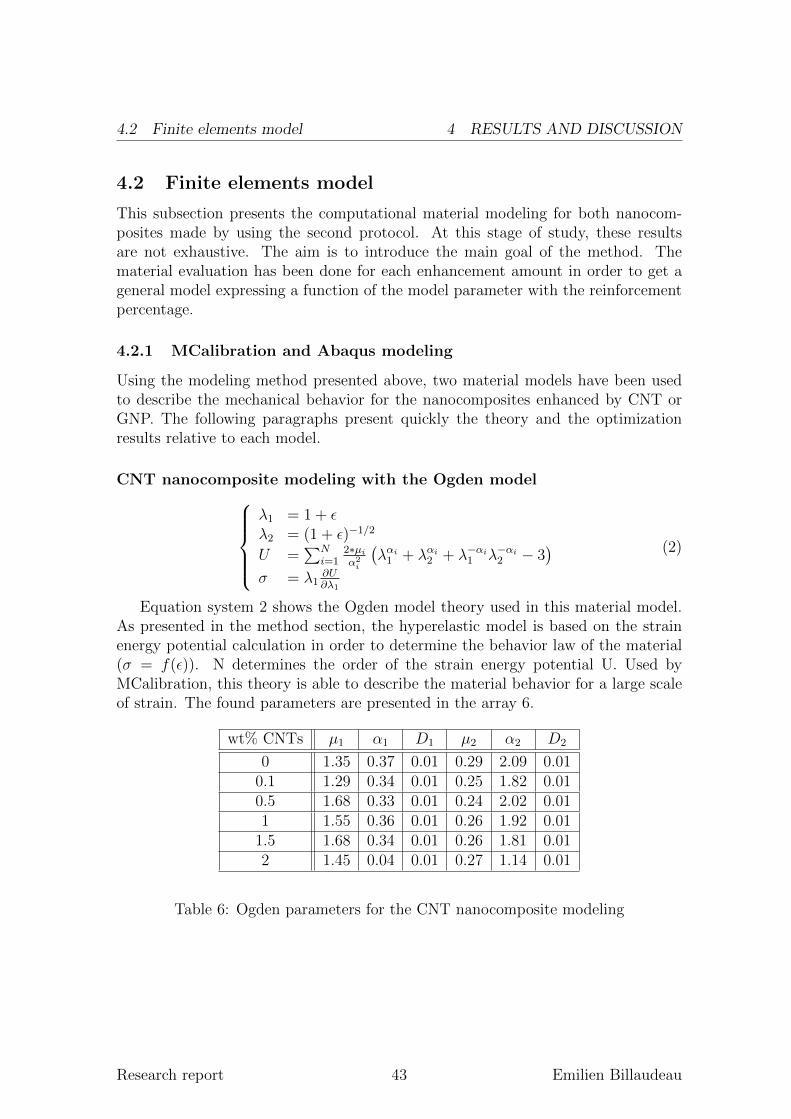
Equation system 2 shows the Ogden model theory used in this material model.As presented in the method section, the hyperelastic model is based on the strainenergy potential calculation in order to determine the behavior law of the material(σ = f(�)). N determines the order of the strain energy potential U. Used byMCalibration, this theory is able to describe the material behavior for a large scaleof strain. The found parameters are presented in the array 6.

wt% CNTs µ1 α1 D1 µ2 α2 D2

0 1.35 0.37 0.01 0.29 2.09 0.010.1 1.29 0.34 0.01 0.25 1.82 0.010.5 1.68 0.33 0.01 0.24 2.02 0.011 1.55 0.36 0.01 0.26 1.92 0.011.5 1.68 0.34 0.01 0.26 1.81 0.012 1.45 0.04 0.01 0.27 1.14 0.01

Table 6: Ogden parameters for the CNT nanocomposite modeling



GNP nanocomposite modeling with the Hyperfoam model

λ1 = 1 + �λ2 = λ3 = (1 + �)−1/2

U =�N

i=12∗µi

α2i

�λαi1 + λαi

2 + λαi3 − 3 + 1

βi∗ (J−αi∗βi − 1)

�

σ = λ1∂U∂λ1

(3)

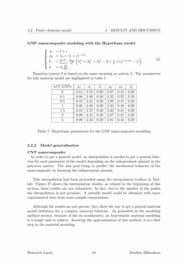
Equation system 3 is based on the same meaning as system 2. The parametersfor this material model are highlighted in table 7.

wt% GNPs µ1 α1 β1 µ2 α2 β2

0 0.12 2.55 0.20 2.07 0.45 0.200.1 0.08 2.46 0.20 2.32 0.35 0.200.5 0.10 2.25 0.20 2.09 0.47 0.201 0.08 2.36 0.20 2.32 0.48 0.201.5 0.10 2.27 0.20 2.30 0.41 0.202 0.09 2.41 0.20 2.87 0.31 0.205 0.06 2.24 0.20 2.81 0.16 0.20

Table 7: Hyperfoam parameters for the GNP nanocomposite modeling

4.2.2 Model generalization

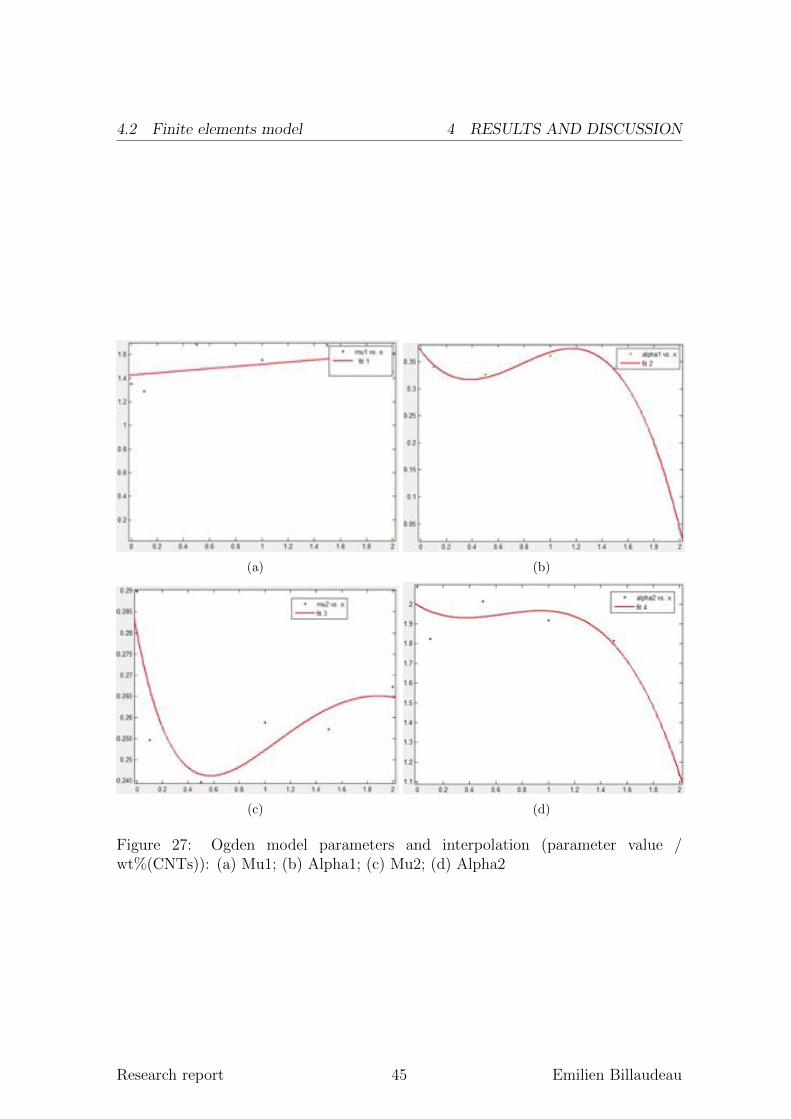
CNT nanocompositeIn order to get a general model, an interpolation is needed to get a general func-

tion for each parameter of the model depending on the enhancement amount in thepolyurea matrix. The aim goal being to predict the mechanical behavior of thenanocomposite by knowing the enhancement amount.

This interpolation had been proceeded using the interpolation toolbox in Mat-lab. Figure 27 shows the interpolation results, as related in the beginning of thissection, these results are not exhaustive. In fact, due to the number of the pointsthe interpolation is not accurate. A suitable model could be obtained with moreexperimental data from more sample compositions.

Although the results are not precise, they show the way to get a general materialmodel definition for a complex material behavior. As presented in the modelingmethod section, because of the its nonlinearity, an hyperelastic material modelingis a tough task to achieve. Knowing the approximation of this method, it is a firststep in the material modeling.



(a) (b)

(c) (d)

Figure 27: Ogden model parameters and interpolation (parameter value /wt%(CNTs)): (a) Mu1; (b) Alpha1; (c) Mu2; (d) Alpha2


5 CONCLUSION

5 Conclusion

In this study we analysed the influence of CNTs and GNPs in Polyurea’s mechanicalbehavior to evaluate the optimal amount of each nanoparticles that yields the bestoverall mechanical performance.

Comparing the results presented above, the nanoparticles dispersion is the mainparameter in the Polyurea enhancement. Without a doubt, the ultrasonic stirring isthe most suitable way to brake the aggregates in order to get a homogenous nanopar-ticles solution. Hence, our first conclusion is that the manufacturing protocol is akey point on the nanomaterial enhancement expectation.

Working on the best suitable manufacturing protocol, we dispersed differentquantities of CNTs and GNPs into the Polyurea matrix to obtain different nanocom-posites with varying mechanical behavior. These tests show that the mechanicalperformance of Polyurea can be significantly enhanced by adding a certain amountof nanoparticles. While we observed substantial enhancement when only 0.5 wt%CNTs or 2 wt% GNPs were added. Adding other quantities gave much weakerperformance in terms of ultimate strength and elongation. Furthermore, comparingthese nanocomposite optimums, the GNP doped-material showed a better behaviorwith a maximum strain and stress. The GNP enhancement corresponded to a rein-forcement twice that of CNT. Hence, our second conclusion is that the amount andthe type of reinforcement should be carefully chosen to get a nanocomposite withthe expected behavior.

Despite the conclusion presented above, due to the time allotted for this research,the temperature effect, the aging impact and the tribology study27 was not studied.These important parameters are required to conclude on material behavior on thespot. In order to finalize this study and to get an appropriate conclusion relatedto the application, Luciana Balsamo, a PhD student at Columbia University willcontinue this research project during her thesis. This thesis will be also providethe opportunity to use and develop the hyperelastic model to find a more suitableevaluation, taking into account the effects introduced above.

27interaction between the nanocomposite layer and the cable


REFERENCES REFERENCES

References

[1] T. Asami and K-H. Nitta. Morphology and mechanical properties of polyolefinicthermoplastic elastomer i. characterization of deformation process. Polymer,45:5301–5306, 2004.

[2] J. Bergstrom. J. PolyUMod, a library of user materials for ABAQUS. VerystEngineering, LLC, 2010.

[3] J. Bergstrom. MCalibration manual. Veryst Engineering, LLC, 2010.

[4] Y. Geng, S. J. Wang, and J-K Kim. Preparation of graphite nanoplatelets andgraphene sheets. Journal of Colloid and Interface Science, 336:592–598, 2009.

[5] Y.H. Ho, C.P. Chang, F.L. Shyu, R.B. Chen, S.C. Chen, and M.F. Lin. Elec-tronic and optical properties of double-walled armchair carbon nanotubes. El-sevier, Carbon, 42:3159–3167, 2004.

[6] S. Iijima. Carbon nanotubes: past, present, and future. Physica B, 323:1–5,2002.

[7] ASTM International. Standard test methods for vulcanized rubber and ther-moplastic elastomers-tension. ASTM International, D412-06a:1–14, 2010.

[8] T. Kuilla, S. Bhadra, D. Yao, N.H. Kim, S. Bose, and J.H. Lee. Recent advancesin graphene based polymer composites. Progress in polymer science, AcceptedManuscrit, 2010.

[9] M. Kulkarni, D. Carnahan, K. Kulkarni, D. Qian, and J. L.Abot. Elastic re-sponse of a carbon nanotube fiber renforced polymeric composite : a numericaland experimental study. Elsevier, B 41:414–421, 2009.

[10] V. Likodimos, S. Glenis, and L. Lin. Electronic properties of boron-dopedmultiwall carbon nanotubes studied by esr and static magnetization. Physical

review, B 72:045436(1–7), 2005.

[11] P.C. Ma, N.A. Siddiqui, G. Marom, and J.K. Kim. Dispersion and function-alization of carbon nanotubes for polymer-based nanocomposites. Composites

Part A: Applied Science and Manufacturing, In Press, Corrected Proof, 2010.

[12] George R. International Journal of Critical Infrastructure Protection, 2008.

[13] C.M. Roland, J.N. Twigg, Y. Vu, and P.H. Mott. High strain rate mechanicalbehavior of polyurea. Elsevier, Polymer, 48:574–578, 2006.

[14] J.P. Salvetat, J.M. Bonard, N.H. Thomson, A.J. Kulik, L. Forro, W. Benoit,and L. Zuppiroli. Mechanical properties of carbon nanotubes. Applied Physics

A, Materials Science and Processing, 69:255–260, 1999.

[15] XG Sciences. Dispersion notes.


REFERENCES REFERENCES

[16] Simula. Abaqus user’s manual. Dassault Systemes, 2010.

[17] R. S.Ruoff, D. Qian, and W. Kam Liu. Mechanical properties of carbonnanotubes : theoretical predictions and experimental measurement. C. R.

Physique, 4:993–1008, 2003.

[18] Technische fakultat der christian albrechts universitat, Kiel. Test M604: Scan-

ning electron microscopy.

[19] H.D. Wagner and R.A. Vaia. Nanocomposites : issues at the interface. Materials

today, 7:38–42, 2004.

[20] M-K. Yeh, T-H. Hsieh, and N-H. Tai. Fabrication and mechanical propertiesof multi-walled carbon nanotubes/epoxy nanocomposites. Elsevier, Material

science and engineering A, 483-484:289–292, 2006.


6 APPENDIX

6 Appendix


6.1 Which solvent for the nanoparticles dispersion 6 APPENDIX

6.1 Which solvent for the nanoparticles dispersion

There is still a long road to create nanoparticle reinforcement composites, fullyrealizing the potential of high strength and stiffness of the CNTs or the GNPs.There are many reasons for this limitation. As presented in the method section,the nanoparticles dispersion is the main point in the nanocomposite manufacturing.This appendix investigates this effect and presents the way to reduce its influence inthe nanocomposite behavior. This study presents the best method to disperse theCNTs (the GNPs dispersion is equivalent).

The CNTs dispersion

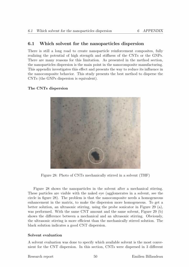
Figure 28: Photo of CNTs mechanically stirred in a solvent (THF)

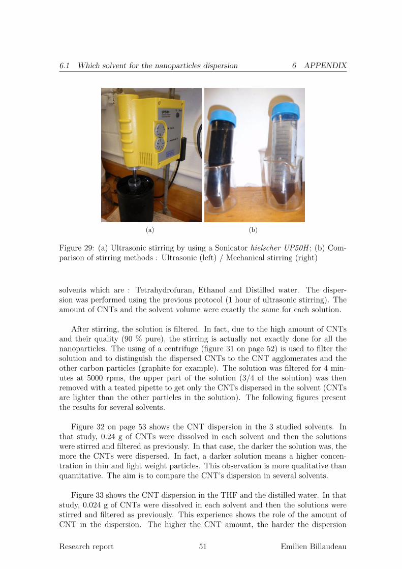
Figure 28 shows the nanoparticles in the solvent after a mechanical stirring.These particles are visible with the naked eye (agglomerates in a solvent, see thecircle in figure 28). The problem is that the nanocomposite needs a homogeneousenhancement in the matrix, to make the dispersion more homogeneous. To get abetter solution, an ultrasonic stirring, using the probe sonicator in Figure 29 (a),was performed. With the same CNT amount and the same solvent, Figure 29 (b)shows the difference between a mechanical and an ultrasonic stirring. Obviously,the ultrasonic stirring is more efficient than the mechanically stirred solution. Theblack solution indicates a good CNT dispersion.

Solvent evaluation

A solvent evaluation was done to specify which available solvent is the most conve-nient for the CNT dispersion. In this section, CNTs were dispersed in 3 different



(a) (b)

Figure 29: (a) Ultrasonic stirring by using a Sonicator hielscher UP50H ; (b) Com-parison of stirring methods : Ultrasonic (left) / Mechanical stirring (right)

solvents which are : Tetrahydrofuran, Ethanol and Distilled water. The disper-sion was performed using the previous protocol (1 hour of ultrasonic stirring). Theamount of CNTs and the solvent volume were exactly the same for each solution.

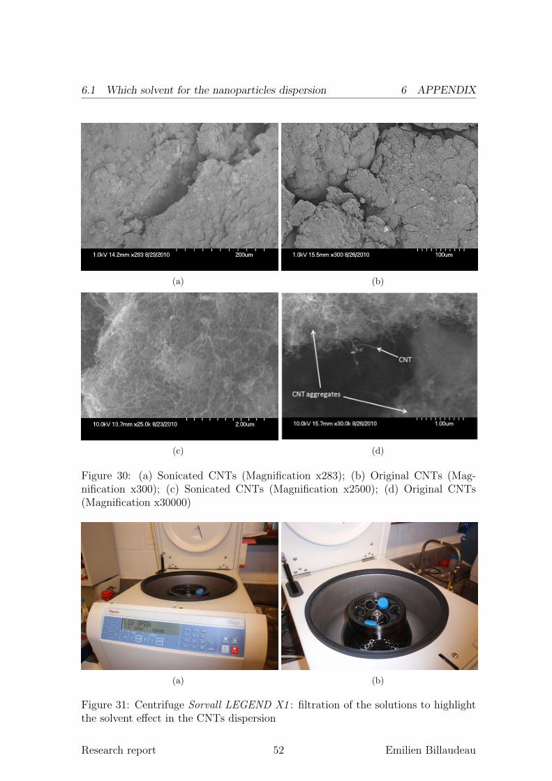
After stirring, the solution is filtered. In fact, due to the high amount of CNTsand their quality (90 % pure), the stirring is actually not exactly done for all thenanoparticles. The using of a centrifuge (figure 31 on page 52) is used to filter thesolution and to distinguish the dispersed CNTs to the CNT agglomerates and theother carbon particles (graphite for example). The solution was filtered for 4 min-utes at 5000 rpms, the upper part of the solution (3/4 of the solution) was thenremoved with a teated pipette to get only the CNTs dispersed in the solvent (CNTsare lighter than the other particles in the solution). The following figures presentthe results for several solvents.

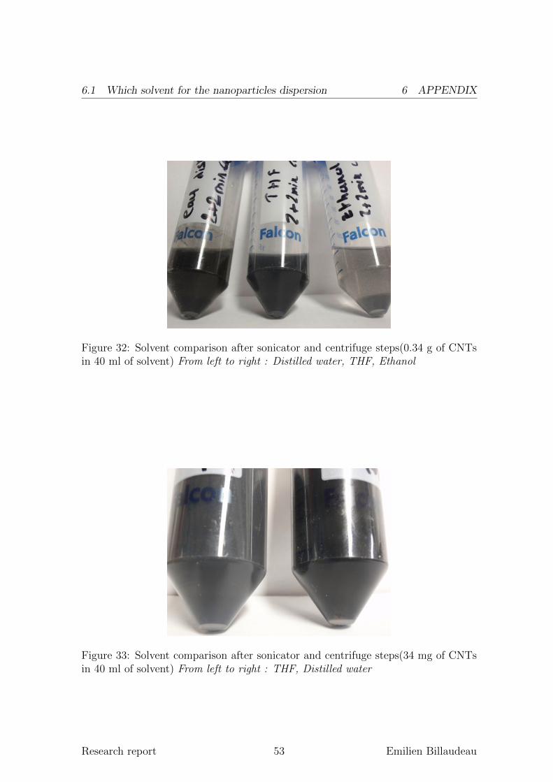
Figure 32 on page 53 shows the CNT dispersion in the 3 studied solvents. Inthat study, 0.24 g of CNTs were dissolved in each solvent and then the solutionswere stirred and filtered as previously. In that case, the darker the solution was, themore the CNTs were dispersed. In fact, a darker solution means a higher concen-tration in thin and light weight particles. This observation is more qualitative thanquantitative. The aim is to compare the CNT’s dispersion in several solvents.

Figure 33 shows the CNT dispersion in the THF and the distilled water. In thatstudy, 0.024 g of CNTs were dissolved in each solvent and then the solutions werestirred and filtered as previously. This experience shows the role of the amount ofCNT in the dispersion. The higher the CNT amount, the harder the dispersion



(a) (b)

(c) (d)

Figure 30: (a) Sonicated CNTs (Magnification x283); (b) Original CNTs (Mag-nification x300); (c) Sonicated CNTs (Magnification x2500); (d) Original CNTs(Magnification x30000)

(a) (b)

Figure 31: Centrifuge Sorvall LEGEND X1 : filtration of the solutions to highlightthe solvent effect in the CNTs dispersion



Figure 32: Solvent comparison after sonicator and centrifuge steps(0.34 g of CNTsin 40 ml of solvent) From left to right : Distilled water, THF, Ethanol

Figure 33: Solvent comparison after sonicator and centrifuge steps(34 mg of CNTsin 40 ml of solvent) From left to right : THF, Distilled water



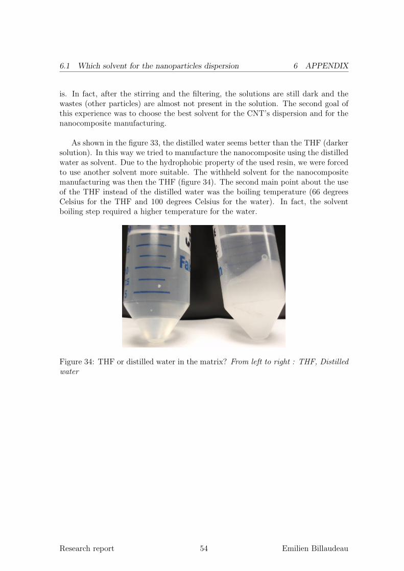
is. In fact, after the stirring and the filtering, the solutions are still dark and thewastes (other particles) are almost not present in the solution. The second goal ofthis experience was to choose the best solvent for the CNT’s dispersion and for thenanocomposite manufacturing.

As shown in the figure 33, the distilled water seems better than the THF (darkersolution). In this way we tried to manufacture the nanocomposite using the distilledwater as solvent. Due to the hydrophobic property of the used resin, we were forcedto use another solvent more suitable. The withheld solvent for the nanocompositemanufacturing was then the THF (figure 34). The second main point about the useof the THF instead of the distilled water was the boiling temperature (66 degreesCelsius for the THF and 100 degrees Celsius for the water). In fact, the solventboiling step required a higher temperature for the water.

Figure 34: THF or distilled water in the matrix? From left to right : THF, Distilled

water


6.2 Strain rate in the rubber materials 6 APPENDIX

6.2 Strain rate in the rubber materials

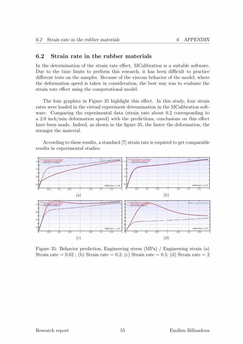
In the determination of the strain rate effect, MCalibration is a suitable software.Due to the time limits to perform this research, it has been difficult to practicedifferent tests on the samples. Because of the viscous behavior of the model, wherethe deformation speed is taken in consideration, the best way was to evaluate thestrain rate effect using the computational model.

The four graphics in Figure 35 highlight this effect. In this study, four strainrates were loaded in the virtual experiment determination in the MCalibration soft-ware. Comparing the experimental data (strain rate about 0.2 corresponding toa 2.0 inch/min deformation speed) with the predictions, conclusions on this effecthave been made. Indeed, as shown in the figure 35, the faster the deformation, thestronger the material.

According to these results, a standard [7] strain rate is required to get comparableresults in experimental studies.

(a) (b)

(c) (d)

Figure 35: Behavior prediction, Engineering stress (MPa) / Engineering strain (a)Strain rate = 0.02 ; (b) Strain rate = 0.2; (c) Strain rate = 0.5; (d) Strain rate = 2


6.3 Interaction between MCalibration and Abaqus 6 APPENDIX

6.3 Interaction between MCalibration and Abaqus

Figure 36: Modeling method using a MCalibration input file


6.4 Matlab smoothing program 6 APPENDIX

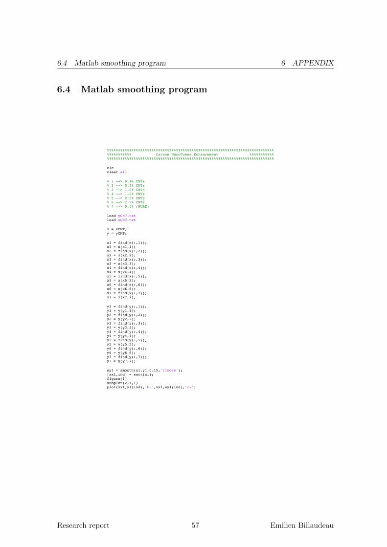
6.4 Matlab smoothing program

%%%%%%%%%%%%%%%%%%%%%%%%%%%%%%%%%%%%%%%%%%%%%%%%%%%%%%%%%%%%%%%%%%%%%%%%%%% %%%%%%%%%%% Carbon NanoTubes Enhancement %%%%%%%%%%% %%%%%%%%%%%%%%%%%%%%%%%%%%%%%%%%%%%%%%%%%%%%%%%%%%%%%%%%%%%%%%%%%%%%%%%%%%% clc clear all % 1 --> 0.1% CNTs % 2 --> 0.5% CNTs % 3 --> 1.0% CNTs % 4 --> 1.5% CNTs % 5 --> 2.0% CNTs % 6 --> 2.5% CNTs % 7 --> 0.0% (PURE) load yCNT.txt load xCNT.txt x = xCNT; y = yCNT; x1 = find(x(:,1)); x1 = x(x1,1); x2 = find(x(:,2)); x2 = x(x2,2); x3 = find(x(:,3)); x3 = x(x3,3); x4 = find(x(:,4)); x4 = x(x4,4); x5 = find(x(:,5)); x5 = x(x5,5); x6 = find(x(:,6)); x6 = x(x6,6); x7 = find(x(:,7)); x7 = x(x7,7); y1 = find(y(:,1)); y1 = y(y1,1); y2 = find(y(:,2)); y2 = y(y2,2); y3 = find(y(:,3)); y3 = y(y3,3); y4 = find(y(:,4)); y4 = y(y4,4); y5 = find(y(:,5)); y5 = y(y5,5); y6 = find(y(:,6)); y6 = y(y6,6); y7 = find(y(:,7)); y7 = y(y7,7); sy1 = smooth(x1,y1,0.15,'rloess'); [xx1,ind] = sort(x1); figure(1) subplot(2,1,1) plot(xx1,y1(ind),'b.',xx1,sy1(ind),'r-')



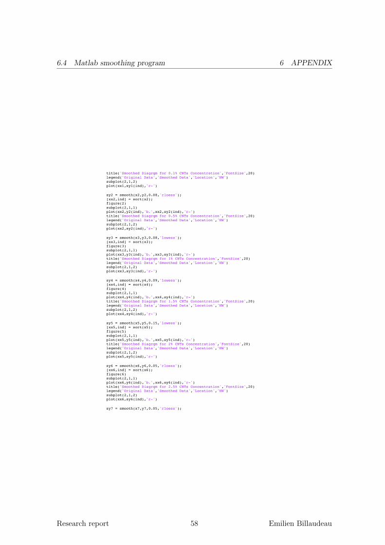
title('Smoothed Diagrqm for 0.1% CNTs Concentration','FontSize',20) legend('Original Data','Smoothed Data','Location','NW') subplot(2,1,2) plot(xx1,sy1(ind),'r-') sy2 = smooth(x2,y2,0.08,'rloess'); [xx2,ind] = sort(x2); figure(2) subplot(2,1,1) plot(xx2,y2(ind),'b.',xx2,sy2(ind),'r-') title('Smoothed Diagrqm for 0.5% CNTs Concentration','FontSize',20) legend('Original Data','Smoothed Data','Location','NW') subplot(2,1,2) plot(xx2,sy2(ind),'r-') sy3 = smooth(x3,y3,0.08,'lowess'); [xx3,ind] = sort(x3); figure(3) subplot(2,1,1) plot(xx3,y3(ind),'b.',xx3,sy3(ind),'r-') title('Smoothed Diagrqm for 1% CNTs Concentration','FontSize',20) legend('Original Data','Smoothed Data','Location','NW') subplot(2,1,2) plot(xx3,sy3(ind),'r-') sy4 = smooth(x4,y4,0.09,'lowess'); [xx4,ind] = sort(x4); figure(4) subplot(2,1,1) plot(xx4,y4(ind),'b.',xx4,sy4(ind),'r-') title('Smoothed Diagrqm for 1.5% CNTs Concentration','FontSize',20) legend('Original Data','Smoothed Data','Location','NW') subplot(2,1,2) plot(xx4,sy4(ind),'r-') sy5 = smooth(x5,y5,0.15,'lowess'); [xx5,ind] = sort(x5); figure(5) subplot(2,1,1) plot(xx5,y5(ind),'b.',xx5,sy5(ind),'r-') title('Smoothed Diagrqm for 2% CNTs Concentration','FontSize',20) legend('Original Data','Smoothed Data','Location','NW') subplot(2,1,2) plot(xx5,sy5(ind),'r-') sy6 = smooth(x6,y6,0.05,'rloess'); [xx6,ind] = sort(x6); figure(6) subplot(2,1,1) plot(xx6,y6(ind),'b.',xx6,sy6(ind),'r-') title('Smoothed Diagrqm for 2.5% CNTs Concentration','FontSize',20) legend('Original Data','Smoothed Data','Location','NW') subplot(2,1,2) plot(xx6,sy6(ind),'r-') sy7 = smooth(x7,y7,0.05,'rloess');



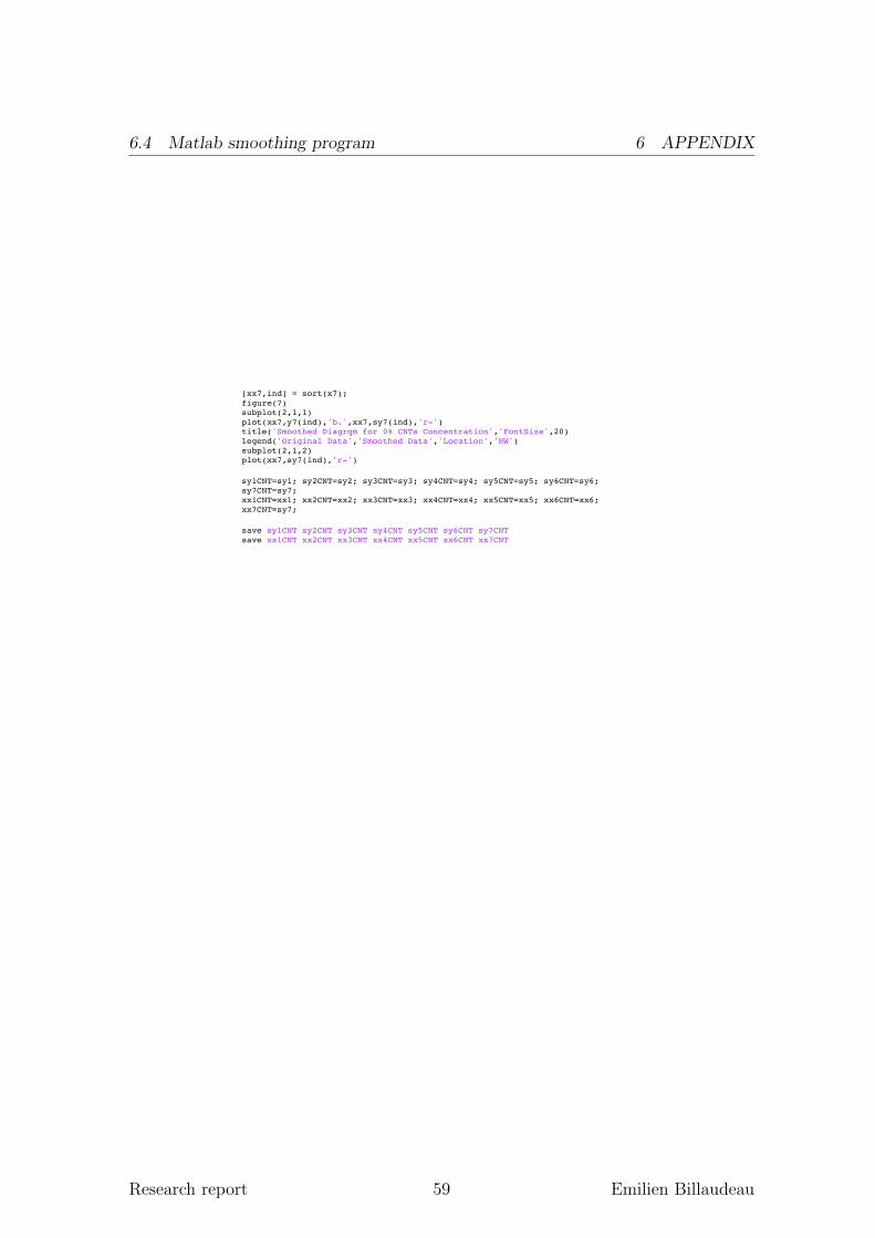
[xx7,ind] = sort(x7); figure(7) subplot(2,1,1) plot(xx7,y7(ind),'b.',xx7,sy7(ind),'r-') title('Smoothed Diagrqm for 0% CNTs Concentration','FontSize',20) legend('Original Data','Smoothed Data','Location','NW') subplot(2,1,2) plot(xx7,sy7(ind),'r-') sy1CNT=sy1; sy2CNT=sy2; sy3CNT=sy3; sy4CNT=sy4; sy5CNT=sy5; sy6CNT=sy6; sy7CNT=sy7; xx1CNT=xx1; xx2CNT=xx2; xx3CNT=xx3; xx4CNT=xx4; xx5CNT=xx5; xx6CNT=xx6; xx7CNT=sy7; save sy1CNT sy2CNT sy3CNT sy4CNT sy5CNT sy6CNT sy7CNT save xx1CNT xx2CNT xx3CNT xx4CNT xx5CNT xx6CNT xx7CNT !


mechanical behavior of polyurea … · scientifiques de niveau recherche, ... mechanical behavior...

Documents